Abstract
The International Energy Agency Technology Collaboration Programme for Ocean Energy Systems (OES) initiated the OES Wave Energy Conversion Modelling Task, which focused on the verification and validation of numerical models for simulating wave energy converters (WECs). The long-term goal is to assess the accuracy of and establish confidence in the use of numerical models used in design as well as power performance assessment of WECs. To establish this confidence, the authors used different existing computational modelling tools to simulate given tasks to identify uncertainties related to simulation methodologies: (i) linear potential flow methods; (ii) weakly nonlinear Froude–Krylov methods; and (iii) fully nonlinear methods (fully nonlinear potential flow and Navier–Stokes models). This article summarizes the code-to-code task and code-to-experiment task that have been performed so far in this project, with a focus on investigating the impact of different levels of nonlinearities in the numerical models. Two different WECs were studied and simulated. The first was a heaving semi-submerged sphere, where free-decay tests and both regular and irregular wave cases were investigated in a code-to-code comparison. The second case was a heaving float corresponding to a physical model tested in a wave tank. We considered radiation, diffraction, and regular wave cases and compared quantities, such as the WEC motion, power output and hydrodynamic loading.
1. Introduction
The development of wave energy converters (WECs) relies on numerical simulations to optimize and evaluate their designs and provide the power performance estimates that feed into the levelized cost of energy (LCOE). The reliability and accuracy of the numerical tools used is therefore of paramount importance. The “performance before readiness” path, put forward by Weber [1], argues that it is most economical to make the optimization and major design choices early in the development process to achieve a high technology performance level, which indicates a low LCOE, before building and deploying a costly WEC at a higher technology readiness level. The “performance before readiness” path requires iterations of optimizations using numerical tools and validations using small-scale physical tests, and thus the confidence in the numerical tools must not be questioned.
The numerical tools of the trade are based on the linearized potential flow theory, thereby solving the Cummins’ equation [2] describing the motion of the WEC. These models are firmly established in the marine engineering sector and have successfully been used for decades (e.g., in oil and gas industries). Well-known commercial codes are OrcaFlex [3], DeepC [4], and ANSYS Aqwa [5], to name just a few. For some wave energy applications—such as point absorbers working in resonance, overtopping devices or WECs under parametric excitation—parts of the underlying assumptions of linear potential flow are violated. So, we must ask the question: how well can these devices still be modelled with standard linear tools? Furthermore, the power take-off (PTO) mechanisms and any control strategies are typically not included “off the shelf” in the commercial packages (but can be implemented through user-defined functions), therefore spurring the development of dedicated wave energy tools based on linearized potential flow theory (e.g., WEC-Sim [6] and InWave [7]).
In recent years, there has been an increased interest in nonlinear hydrodynamic modelling of wave energy converters, and there are several approaches. The weakly nonlinear Froude–Krylov (FK) approach [8] is the most used and has been implemented in several of the existing linear codes, extending them to weakly nonlinear tools. The use of fully nonlinear potential flow (FNPF) is still rather scarce [9], but computational fluid dynamics (CFD) tools are frequently used [10]. However, the computational complexity and cost still hinders the use of high-fidelity tools for everyday engineering tasks in wave energy.
There is a need for solid verification and validation of numerical codes used in wave energy applications, with regard to both how the overall level of fidelity depends on the hydrodynamic model, and how different choices within each sub-category affect the accuracy and reliability of the computed results. Examples of different approaches to implementing the nonlinear FK force can be found in [11,12]. Other questions not yet fully answered are how the choices of fidelity levels within subsystems, such as the PTO [12] and the mooring system [13], influence the results, as well as how the inclusion of control strategies affects the reliability of the simulations. Investigation of these questions is the aim of the Ocean Energy Systems (OES) wave energy conversion modelling task on the verification and validation of simulation tools for wave energy systems.
1.1. The Background of the OES Wave Energy Conversion Modelling Verification and Validation Task
OES is one of the Technology Collaboration Programmes (TCPs) under the International Energy Agency (IEA). OES was founded in 2001 by Denmark, the United Kingdom, and Portugal, and currently has 25 member countries that cooperate on different tasks related to ocean energy. The OES WEC modelling verification and validation task was inspired by the successful work on code validation performed in the IEA Wind TCP Task 23 and 30 for offshore wind turbines under the acronyms OC3, OC4 and OC5 [14,15,16]. To inform the OES on the task on Ocean Energy Modelling Verification and Validation, eight participants were brought together in the WEC3 (Wave Energy Converter Code Comparison) project. All participants used mid-fidelity (time-domain, weakly nonlinear solvers) modeling an oscillating flap device [17]. It was found that the solutions generally matched, but that the choice of viscous correction could yield significant differences.
The OES Executive Committee approved the OES WEC modelling verification and validation task in 2016 with the overall goal to assess the accuracy of the numerical models used, and to improve confidence in these codes. Participation is open to all interested partners, with a total of 29 organizations from 13 countries participating in the project thus far. The participants include universities, research laboratories, commercial software developers, consultants and WEC developers. The numerical models range from linear and weakly nonlinear models, and fully nonlinear time-domain boundary element methods (BEM), to computational fluid dynamics (CFD) solvers. Fully nonlinear solvers have been used in the wave energy sector for some time now, as described in some early studies [18,19,20,21] and have been incorporated in the OES WEC modeling tasks described in this paper.
The work in the OES WEC modeling task is, so far, mainly focused on operational conditions, concentrating on a range of regular wave cases and long-term irregular sea states. Complimentary work is being undertaken in the Collaborative Computational Project in Wave Structure Interaction [22], in which members from the wider wave structure interaction community have been participating in blind comparative studies involving the interaction of focused wave events with various surface-piercing structures.
1.2. Paper Contribution
This article reviews two numerical experiments provided by the team of project participants with the objective of investigating the code-to-code task and code-to-experiment task that have been performed so far in this project. We focus on investigating the impact of different levels of nonlinearities in numerical models. Further, we will discuss the advantages, disadvantages and the range of validity of the different methods and tools studied. The first code-to-code comparison of a heaving sphere is described in a joint reference paper [23] and a follow-up paper that includes simulations on power performance and calculation of energy production [24]. The second part of this paper describes validation using existing experimental data presented for the first time.
2. Description of the Numerical Tools
The dynamic response of the system is calculated by solving the system’s equations of motion. The equation of motion for a floating body can be expressed as:
where is the (translational and rotational) acceleration vector of the body, is the mass matrix, is the total hydrodynamic (including hydrostatic and gravitational restoring) force vector, and is the external force vector (e.g., PTO, mooring, and multibody constraint forces). The hydrodynamic forces on the floating body are calculated using linear, weakly nonlinear, or fully nonlinear methods. A brief summary of each approach is described in this section.
2.1. Linear Models
Linear models are commonly used to model WECs. The model is based on linear wave theory, in which the waves are assumed to be a linear superposition of incident, radiated, and diffracted wave components. The total hydrodynamic force in Equation (1) is expressed as:
where , and are the vectors of radiation forces, wave-excitation forces, and net buoyancy restoring forces. Table 1 lists the linear models used in the study.

Table 1.
List of linear models.
The buoyancy restoring term includes the hydrostatic and gravitational restoring forces. The radiation term includes added-mass and radiation damping components, proportional to the acceleration and velocity of the floating body, respectively. The hydrodynamic radiation force, as a function of time, can be calculated using a convolution integral of the impulse response function (IRF) or using a state–space (SS) approach as an approximation of the integral. The wave excitation term includes an FK force component generated by the undisturbed incident waves and a scattering term that results from the presence of the body. In the irregular wave cases, the total excitation force can be calculated by inverse fast Fourier transform of the product of the excitation force coefficients and the wave spectrum (WS) or by a convolution integral to obtain the wave exciting force from the given incident wave elevation (WE). The added-mass, radiation damping, wave excitation, and hydrostatic restoring coefficients are provided by a frequency-domain BEM solver, either WAMIT [25] or NEMOH [26].
2.2. Weakly Nonlinear Models
The linear model assumes that the body motion and the waves are of small amplitude in comparison to the wavelength. A weakly-nonlinear calculation uses an approach similar to a linear model (Equation (2)) but accounts for the nonlinear buoyancy and the FK forces induced by the instantaneous water surface elevation and body position. Table 2 lists the weakly nonlinear models used in the study.
Table 2.
List of weakly nonlinear models.
Although the scattering excitation force is still linear and computed from the BEM model, the FK excitation term is computed based on the exact body geometry and position and the pressures induced by the incident wave elevation. The hydrostatic forces are also computed using the exact geometry and the incident wave elevation. The incident wave elevation and pressure can be calculated based on linear or higher-order wave theory. If linear wave theory is used to determine the flow velocity and pressure field, the values become unrealistically large for wetted panels that are above the mean water level. To correct this, a wave stretching method was applied with a correction to the instantaneous wave elevation that forces its height to be equal to the water depth when calculating the flow velocity and pressure.
2.3. Fully Nonlinear Models
The fully nonlinear model tracks the free surface in the time domain and calculates the hydrodynamic force vector based on the integration of total pressure over the body surface in the fluid domain at each time step, i.e.:
where p is the total pressure, is the shear force vector, n is the unit normal vector, and r is the vector between the center of each surface panel and the body’s center of gravity. Table 3 lists the fully nonlinear models used in the study.
Table 3.
List of fully nonlinear models.
Two types of fully nonlinear models are used in the study. One is the fully nonlinear potential flow (FNPF) method, for which , since the flow is assumed to be inviscid. Using a time-domain BEM approach, the computational domain is discretized along the domain boundaries, including the free surface and the body surface. A surface tracking method is used to predict the free surface, and the velocity potential is solved in the time domain. The method is capable of fully accounting for the influence of nonlinear waves on the body dynamics up to a point close to wave breaking.
The other type is the unsteady Navier–Stokes-method-based CFD models, which fully predict the effects of boundary layer viscous flow separation and turbulence. Typically, in wave energy applications, the turbulence is statistically averaged and the Reynolds-averaged Navier–Stokes equations are most often discretized using the finite volume method (FVM). Another more recent approach to turbulence modelling is to let the turbulence be modelled by a weak form of a stabilized finite element method (FEM). This parameter-free residual-based sub-grid approach, which can be considered as an implicit large-eddy simulation (iLES), is denoted as direct finite element simulation (DFES). All models solve the two-phase air/water problem and are capable of capturing wave breaking and overtopping in the hydrodynamic model. Most of the models rely on the volume of fluid (VOF) approach to capture the free surface elevation but the level set (LS) method is also used.
3. Code-to-Code Comparison of a Heaving Semi-Submerged Sphere
We chose a heaving semi-submerged sphere as the first test case. The dimensions, properties, and the coordinate system used are shown in Figure 1. For all cases, the global coordinate system is aligned at the still water level, with the z-axis pointing upward. The sphere is constrained to move in heave only. The heave natural period of the sphere is given by the following formula [27]:
where g is the acceleration caused by gravity and a is the sphere radius. This gives a s. The hydrodynamic coefficients (added-mass, radiation damping, and wave exciting force) calculated using both WAMIT [25] and NEMOH [26] were supplied to the participants.
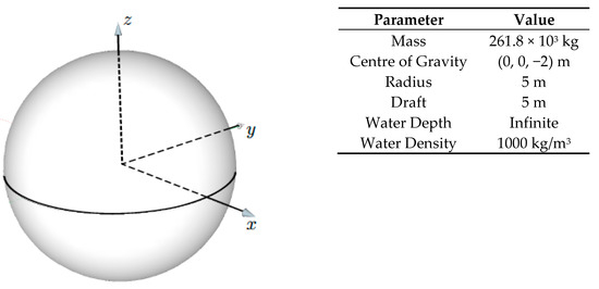
Figure 1.
Sketch and general properties of the heaving sphere case.
3.1. Decay Tests
The initial test specified for the participants was the hydrostatic and heave decay test. The hydrostatic test ensures that, at its mean position, exactly half of the sphere is submerged. Three initial displacements were specified for the decay tests: 1 m, 3 m, and 5 m. The 5-m displacement case corresponds to the sphere initially just touching the mean free surface. No PTO damping was considered in the decay tests. The participants were asked to submit 40 s of simulation results.
The impact of nonlinearities on the response of the heaving sphere during a heave free decay test is illustrated in Figure 2, which shows the heave decay of the sphere when released from an initial displacement of 5 m, which is equal to the mean draft and radius of the sphere.
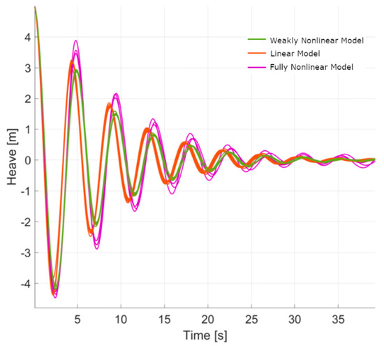
Figure 2.
Simulated heave decay of the sphere from an initial displacement of 5 m. Differences between linear and nonlinear models are clear.
Differences in the response obtained from the three different groups of numerical models are clear in this case. Comparing the response predicted by linear models (red) to those predicted by weakly nonlinear models (green), one can observe differences in terms of phasing and amplitude. These differences can be attributed to variations in the hydrostatic stiffness when the sphere moves in the heave direction.
The purple group of models includes unsteady Reynolds-averaged Navier–Stokes (URANS) models and a fully nonlinear time-domain potential flow code. In addition to capturing the effect of nonlinear hydrostatic effects, these CFD tools also capture nonlinearities related to radiated waves. For an initial displacement of 5 m, the CFD models predict a breaking radiated wave, which impacts the motion response of the heaving sphere.
The weakly nonlinear (green) and fully nonlinear (purple) models predict approximately the same heave natural period. However, it is surprising to see that the fully nonlinear models predict higher response amplitudes than both the linear and weakly nonlinear models. For decay cases with smaller initial displacements, the agreement between linear and nonlinear models tends to improve. More discussion on this topic is given in [23].
3.2. Regular Waves
In total, 10 different wave periods were considered. We considered three wave steepness values (i.e., 0.0005, 0.002, and 0.01) and three model configurations (i.e., free, fixed, and with optimum PTO damping) for each wave period, yielding a total of 90 regular wave simulations. The participants were asked to submit 150 s of steady-state simulation results. Because of the large computational expenses associated with the CFD tools that consider strong nonlinearities, we considered only linear and weakly nonlinear models for the regular wave simulations. Figure 3 shows the heave motion response amplitude operator (RAO) and the mean power obtained with optimum PTO damping for the regular wave conditions outlined in Table 4.
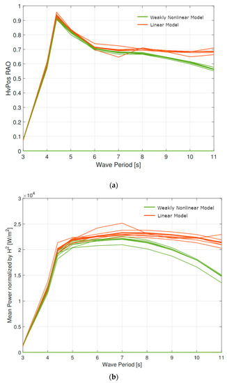
Figure 3.
(a) Heave RAO and (b) mean power normalized by the square of the wave height, for the heaving sphere in regular waves with steepness S = 0.01 and optimum PTO damping.
Table 4.
Regular wave conditions.
We selected the wave heights, H, to give the same wave steepness, S = 0.01, for all of the regular wave conditions considered, where S is defined as:
The value S = 0.01 is equivalent to which is about half the maximum possible value for progressive waves in deep water, . The RAO for each regular wave condition is computed as:
with being the fundamental peak of the heave-motion power spectral density (PSD) and being the fundamental peak of the wave elevation PSD.
For this optimum PTO damping case, linear and weakly nonlinear codes show reasonable agreement for wave periods below 6 s (including the resonance period of 4.4 s); however, for wave periods beyond 6 s, the heave motion and consequently the power predictions of the linear and weakly-nonlinear models start to diverge. This divergence is caused by geometric nonlinearities related to the spherical shape, which introduce nonlinear hydrostatic and FK forces for larger waves.
3.3. Irregular Waves
The irregular wave elevation time series, generated based on a Pierson–Moskowitz spectrum, were provided to the participants. Initially, three different irregular wave conditions, as shown in Table 5, were analyzed. The first sea state has a peak spectral period that is longer than the heave resonance period of the sphere. For the second sea state, the spectral period is at the heave resonance period of the sphere. The third sea state represents a survival condition, with larger waves and increased steepness. For each irregular wave condition, the participants submit 800 s of simulation results (including initial transients) for three different configurations: free floating, prescribed PTO damping, and fixed.
Table 5.
Irregular wave conditions and selected PTO damping coefficients for the first irregular wave simulation task of the heaving sphere.
For the irregular sea states, the wave steepness, S, is as defined as in Equation (5), with H and T replaced by and , respectively. For the low steepness (S = 0.0026) conditions, we observed no significant differences between the linear and the weakly nonlinear models. For the sea state with increased steepness (S = 0.0047), the weakly nonlinear models predict a reduced motion response around the resonance frequency of the system. This reduced resonance response yields a mean power prediction that is about 20% below the mean power predicted by the linear models. Additional details on the irregular wave analysis are covered in [23].
The second task with irregular sea states includes comparing power-generation calculations in six irregular sea states with optimal linear damping and the same calculations with negative springs. The annual energy production of the heaving sphere was calculated following the simplified methodology of Nielsen and Pontes [28]. This methodology reduces the scatter diagram to the distribution of six sea states with a linear relationship between the significant wave height, and the spectral peak period, , and a specified occurrence in percent. We chose the North Sea, with an average wave power resource of 20 kW/m. The participants were asked to submit 1500 s of simulation results, in addition to the calculated average power production. The annual average absorbed power (with optimal PTO damping but without negative spring) obtained from the participants has a group average of 47.9 kW, with a maximum of 49.3 kW, a minimum of 46.4 kW, and a standard deviation 1.07 kW. In most cases, the differences in results can be caused by truncation of the time series. More detailed discussions can be found in [24].
4. Validation Using Existing Experimental Data of a Heaving Float
The second project phase focused on validation using existing experimental data, which originates from a testing campaign led by Sandia National Laboratories, as described in [29]. The float is a surface-piercing body with a cylinder on top and a conical frustum on the bottom. The dimensions and properties of the 1/7-scale model are given in Figure 4. All information presented here is given in model scale. The hydrodynamic coefficients of the float were computed using WAMIT and supplied to the participants. The natural period of the floater is roughly 0.6 Hz.
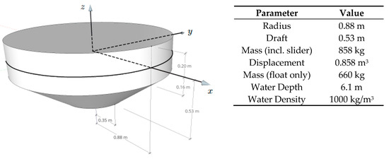
Figure 4.
Sketch and general properties of the heaving float case.
4.1. Decay Tests
No experimental data were available to verify the decay test. However, as in the heaving sphere case, hydrostatic and heave decay tests were performed to ensure that all participants had similar setups and that the models are performing as expected. The participants were asked to submit 100 s of simulation results.
Two different free decay tests are discussed here: one with an initial displacement of 0.1 m and the other with an initial displacement of 0.2 m. Compared to the free decay simulations of the spherical float (Section 3.1), geometric nonlinearities play a much smaller role because the water plane area is constant for heave displacements < 0.16 m (see Figure 4).
As expected, almost all linear and weakly nonlinear codes predict the same free decay response. The fully nonlinear time-domain potential flow solution included here (shown in purple) appears to predict different motion amplitudes but aligns relatively well with the linear and weakly nonlinear codes, in terms of frequency and phasing (Figure 5).
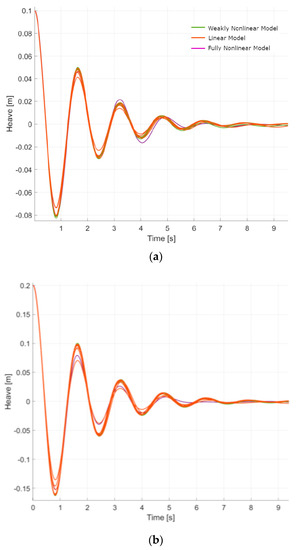
Figure 5.
Free decay simulations of the float in heave. (a) 0.1 m initial displacement and (b) 0.2 m initial displacement.
4.2. Radiation Tests
For the radiation tests, the float was forced to move in otherwise calm water. The goal of these forced oscillation tests was to validate the radiation model. Four tests were specified, with four different oscillation periods. As input to the simulations, the applied actuator force time series were supplied to the participants.
As shown in Figure 6, all codes with their different fidelity levels, in terms of capturing nonlinear effects, agree well with the measured response of the system. For this relatively low frequency and moderate motion amplitude, the device response falls well within the linear regime. For the radiation test shown in Figure 7, the float is being excited at its natural frequency. In this case, the numerical models appear to overpredict the motion response of the float. This is probably related to the influence of viscous effects that often play a larger role for WECs that operate at resonance. For the radiation test case, none of the numerical models included viscous effects. The strongly nonlinear model shown in Figure 7, in purple, is a fully nonlinear time-domain potential flow code.
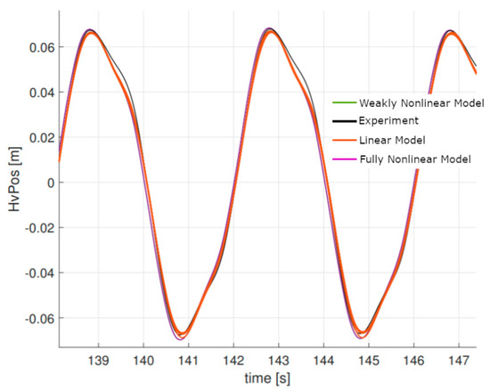
Figure 6.
Radiation test (f = 0.25 Hz, H = 0.0665 m).
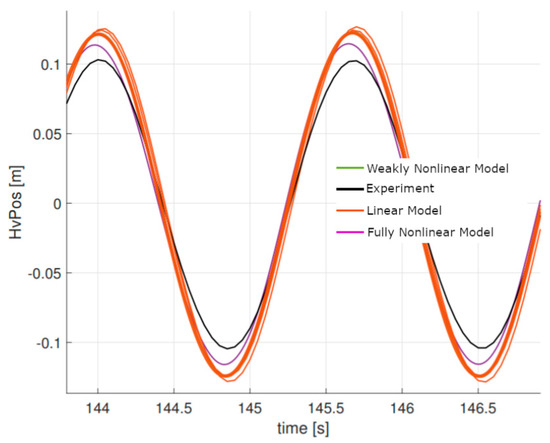
Figure 7.
Radiation test at resonance (f = 0.6 Hz, H = 0.1025 m).
A look at the PSD plot, for the heave motion response at resonance, shows that all codes predict the first-order peak very well, but significantly underpredict the second-order peak at 1.2 Hz (Figure 8). It is interesting to note that the second-order peak is not very prominent in the PSD plot of the actuator force signal that is used to excite the float (Figure 9). As further discussed in Section 4.3, some level of structural compliance was present in the fixture of the heaving float. Whether this second-order peak is related to nonlinear hydrodynamic effects, or to an eigenfrequency of the structure, is difficult to determine.
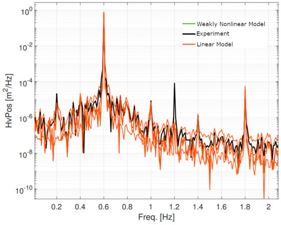
Figure 8.
Radiation test at resonance (f = 0.6 Hz, H = 0.1025 m): heave motion power spectral density (PSD).
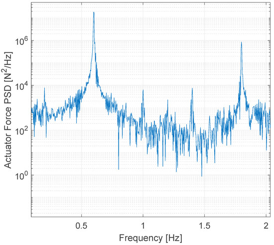
Figure 9.
Radiation test at resonance (f = 0.6 Hz, H = 0.1025 m): actuator force PSD.
4.3. Diffraction Tests
For the diffraction tests, the device was locked in place and subjected to incoming waves. The force measured on the float was used for validation of the numerical diffraction model. In total, four tests with different wave periods and wave heights were specified. As input to the simulations, the wave elevation time series were supplied to the participants.
The simulation time for each case is dictated by the length of the supplied input time series. To estimate the undisturbed wave elevation signal at the location of the model, the phase of the wave was propagated in accordance to the dispersion relation for linear waves. The phase velocity was estimated as:
with h being the water depth and k the wave number. Using Equation (7), the relatively undisturbed wave signal from CarriageSonicNE (see Figure 10) was propagated to the location of the float, as the distance between the wave probe and the float was known (44.307 m).
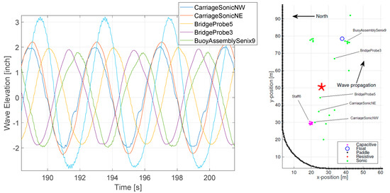
Figure 10.
Comparison of wave elevation signals at different locations for a diffraction test (f = 0.25 Hz, H = 0.10 m) and the wave probe locations in basin.
Figure 10 compares the wave elevation signal measured at different locations in the tank. There is obviously a significant amount of variation, in terms of wave amplitude, depending on the wave probe location. As indicated by the team at Sandia National Laboratories that oversaw the tank testing campaign, a noticeable amount of localized wave reflection was present during the test. These localized reflection effects introduce some level of uncertainty about the actual undisturbed wave elevation at the location of the float. Another major source of uncertainty associated with the test campaign was the structural compliance of the fixture that connects the float to the above bridge. Keeping in mind these uncertainties are related to wave definition and structural compliance, the model validation results must be interpreted with caution.
Figure 11 shows a comparison between linear and weakly nonlinear models with the experimental data for a diffraction test (f = 0.25 Hz, H = 0.10 m). During a diffraction test, the model is held fixed while exposed to wave excitation. The hydrodynamic forces on the float are measured through load cells. As shown in Figure 11, there is obviously a significant discrepancy between the heave force amplitude predicted by the numerical tools and the experimental data. Given the large uncertainty related to the undisturbed wave amplitude at the location of the float, it is hard to determine if the observed differences are caused by deficiencies in the numerical models, or whether the wave elevation was not prescribed correctly for the numerical tools. Looking at the experimental data in Figure 11, we can observe a significant high frequency content in the experimental heave force signal. A PSD plot of the heave force signal for the same diffraction test reveals the excitation of higher order harmonics beyond the first- and second-order response of the system, which can probably be attributed to some level of structural compliance that is present in the model (Figure 12). For the diffraction test illustrated in Figure 11 and Figure 12, linear and weakly nonlinear models are in general agreement.
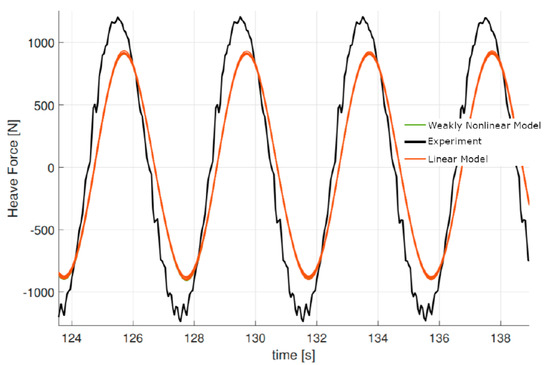
Figure 11.
Heave force acting on the float during a diffraction test (f = 0.25 Hz, H = 0.10 m).
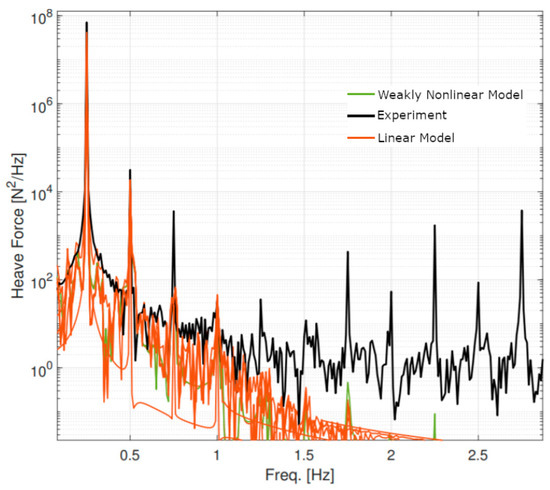
Figure 12.
PSD of heave force acting on the float during a diffraction test (f = 0.25 Hz, H = 0.10 m).
4.4. Regular Waves
We used regular wave tests to obtain the response amplitude operators (RAOs) at various wave periods. Five regular wave test cases were specified with different wave periods but the same wave amplitude (thus different steepness values). The tests were conducted with an active PTO device. To ensure that all participants simulate similar conditions, the PTO force time series and the wave elevation time series were supplied to the participants. As in the radiation and diffraction tests, the simulation time for each case is dictated by the length of the supplied input time series.
The same uncertainties related to the undisturbed wave elevation signal that were discussed for the diffraction test also apply to the regular wave tests. Figure 13 illustrates the heave response for a regular wave test (f = 0.25 Hz, H = 0.10 m). During these regular wave tests, we applied a time varying actuator force, in the heave direction, to the float.
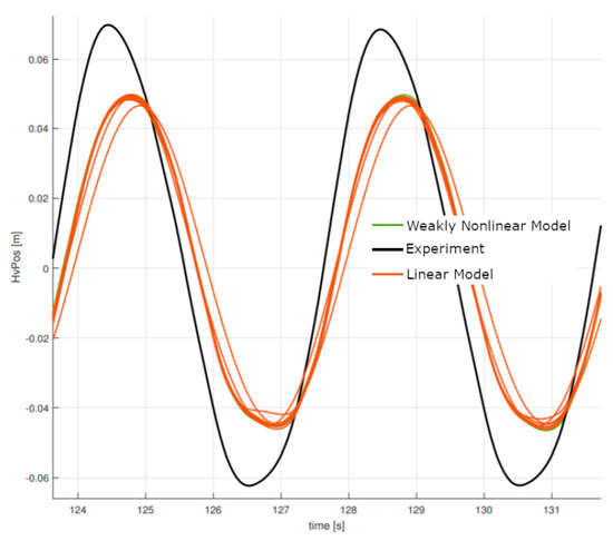
Figure 13.
Heave response during a regular wave case with forced actuation (f = 0.25 Hz, H = 0.10 m).
The underprediction of the heave motion by the numerical tools (Figure 13) is somewhat in line with the underpredicted heave force signal during the diffraction test, shown in (Figure 11), and is probably related to inaccuracies in the prescribed wave amplitude. Judging from the corresponding PSD plot of the heave motion for this regular wave case (Figure 14), we can see that, although the linear and weakly nonlinear models generally under-predict the response of the system and therefore the magnitude of the peaks in the PSD plot, the higher order harmonics are reasonably well resolved by the numerical models, which is likely related to the fact that these harmonics are also present in the actuator force signal, which is also used to drive the float in the simulations.
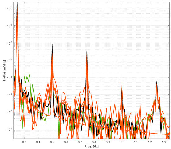
Figure 14.
PSD of the heave response during a regular wave case with forced actuation.
5. Discussion
In this work, we used numerical modelling tools with different levels of fidelity, in terms of capturing nonlinear hydrodynamic effects, to simulate two different heaving bodies. The shape of the sphere introduces nonlinear effects because its water plane area, as well as its wetted surface area, changes when it is displaced in heave. The code-to-code comparison of the heaving sphere revealed the significant impact of geometric nonlinearities on the simulation results. The weakly nonlinear models that consider the instantaneous wetted surface for hydrostatic and FK forces are able to capture the impact of geometric nonlinearities on the response of the system. These nonlinear effects eventually impact the power performance predictions. The nonlinear effects related to the geometry of the sphere were most pronounced for large motions (i.e., heave free decay test with large initial response) and large waves. For model validation, using an experimental heaving float, geometric nonlinearities played a smaller role, as the instantaneous free surface stayed within the cylindrical region of the float (Figure 4). The difficulties that were encountered were related to the inherent uncertainties of the wave basin data set. Linear models appear to be in good agreement with weakly and fully nonlinear models, for the heaving float case.
For both investigated bodies, we observed very good agreement among linear and weakly nonlinear codes. The fundamental principles of these mid-fidelity models are well-understood and their application to model the two heaving bodies investigated within this project phase of IEA OES Wave Energy Modelling Task was a familiar process for the participants. However, we also observed larger differences among the different models that consider strong nonlinearities. Some of these differences can be attributed to the fact that CFD-type models require a lot more input from the user in terms of model definition (e.g., meshing, solver settings, and turbulence models). Some of the differences among the various high-fidelity CFD solutions are also related to the fact that different simplifications were applied to model the flow field (e.g., inviscid and irrotational flow versus URANS-type models). It should also be noted that, for cases including wave breaking, fully nonlinear potential methods show divergent behavior, indicating that the assumption of potential flow is no longer valid. Linear and weakly nonlinear models can, however, be forced to compute solutions that are outside this range. The results should then be used with some caution.
For the longer simulations that involve waves, especially irregular waves, only very few solutions with strong nonlinearities were supplied by the participants, which highlights the limitations regarding the application of CFD tools to simulate a wide range of wave/design conditions. Different wave conditions require mesh refinements in the free-surface area, depending on the wave height and period. Simulating a large number of wave conditions eventually yields a significant amount of work in terms of meshing, which adds to the inherently large computational costs of CFD models.
6. Conclusions
The main result of the study is the similarity of results of using linear, weakly nonlinear and fully nonlinear models in small and medium wave conditions. This is an important result, where linear models can be used instead of computationally costly nonlinear ones.
Author Contributions
K.N. managed the project; F.W. performed the data handling and analysis; F.W., C.E., Y-H.Y., A.K. and K.N. wrote the paper. All authors performed numerical simulations.
Funding
The Danish partners acknowledge the support from the Danish Energy Agency through project 374 64017-05197. The Swedish partners were supported by the Swedish Energy Agency under Grants P44423-1 and 375 P44432-1. J.V.R. and G.G. acknowledge the support by Science Foundation Ireland under Grant 13/IA/1886. This research was made possible by support from U.S. the Department of Energy’s EERE Water Power Technologies Office. Sandia National Laboratories is a multi-mission laboratory managed and operated by National Technology and Engineering Solutions of Sandia, LLC., a wholly owned subsidiary of Honeywell International, Inc., for the U.S. Department of Energy’s National Nuclear Security Administration under contract DE-NA0003525. This work was authored (in part) by the National Renewable Energy Laboratory, operated by Alliance for Sustainable Energy, LLC, for the U.S. Department of Energy (DOE) under Contract No. DE-AC36-08GO28308. Funding was provided by the U.S. Department of Energy Office of Energy Efficiency and Renewable Energy Wind Energy Technologies Office. The views expressed in this article do not necessarily represent the views of the DOE or the U.S. Government. The U.S. Government retains and the publisher, by accepting the article for publication, acknowledge that the U.S. Government retains a non-exclusive, paid-up, irrevocable, worldwide license to publish or reproduce the published form of this work, or allow others to do so, for U.S. Government purposes.
Conflicts of Interest
The authors declare no conflict of interest.
Abbreviations
The following abbreviations are used in this manuscript:
| BEM | boundary element method |
| CFD | computational fluid dynamics |
| DFS | direct finite element simulation |
| FEM | finite element method |
| FK | Froude–Krylov |
| FNPF | fully nonlinear potential flow |
| FVM | finite volume method |
| IEA | International Energy Agency |
| iLES | implicit large eddy simulation |
| IRF | impulse response function |
| LCOE | levelized cost of energy |
| LS | level set |
| OES | Ocean Energy Systems |
| PSD | power spectral density |
| PTO | power take off |
| RAO | response amplitude operator |
| RK4 | 4th-order Runge–Kutta |
| SS | state space |
| SWL | still water level |
| URANS | unsteady Reynolds-averaged Navier–Stokes |
| VOF | volume of fluid |
| WE | wave elevation |
| WEC | wave energy converter |
| WEMT | Wave Energy Modelling Task |
| WS | wave spectrum |
References
- Weber, J. WEC technology readiness and performance matrix-finding the best research technology development trajectory. In Proceedings of the 4th International Conference on Ocean Energy, Dublin, Ireland, 17–19 October 2012. [Google Scholar]
- Cummins, W. The impulse response function and ship motions. Schiffstechnik 1962, 9, 101–109. [Google Scholar]
- OrcaFlex. Available online: https://www.orcina.com/SoftwareProducts/OrcaFlex/ (accessed on 2 May 2019).
- Deep Water Coupled Floater Motion Analysis—DeepC. Available online: https://www.dnvgl.com/services/deep-water-coupled-floater-motion-analysis-deepc-89424 (accessed on 2 May 2019).
- ANSYS Aqwa. Available online: https://www.ansys.com/products/structures/ansys-aqwa (accessed on 2 May 2019).
- Yu, Y.; Lawson, M.; Ruehl, K.; Michelen, C. Development and Demonstration of the WEC-Sim Wave Energy Converter Simulation Tool. In Proceedings of the 2nd Marine Energy Technology Symposium, Washington, DC, USA, 15–17 April 2014. [Google Scholar]
- Combourieu, A.; Philippe, M.; Rongère, F.; Babarit, A. InWave: A new flexible design tool dedicated to wave energy converters. In Proceedings of the 33rd International Conference on Ocean, Offshore and Arctic Engineering, San Francisco, CA, USA, 8–13 June 2014. [Google Scholar]
- Giorgi, G.; Ringwood, J.V. Nonlinear Froude-Krylov and viscous drag representations for wave energy converters in the computation/fidelity continuum. Ocean Eng. 2017, 141, 164–175. [Google Scholar] [CrossRef]
- Fitzgerald, C. Nonlinear Potential Flow Models. In Numerical Modelling of Wave Energy Converters: State-of-the Art Techniques for Single WEC and Converter Arrays; Folley, M., Ed.; Academic Press: Cambridge, MA, USA, 2016; pp. 83–104. [Google Scholar]
- Windt, C.; Davidson, J.; Ringwood, J.V. High-fidelity numerical modelling of ocean wave energy systems: A review of computational fluid dynamics-based numerical wave tanks. Renew. Sustain. Energy Rev. 2018, 93, 610–630. [Google Scholar] [CrossRef]
- Gilloteaux, J.C.; Ducrozet, G.; Babarit, A.; Clément, A. Non-linear model to simulate large amplitude motions: Application to wave energy conversion. In Proceedings of the 22nd International Workshop on Water Waves and Floating Bodies, Plitvice Lakes, Croatia, 15–18 April 2007. [Google Scholar]
- Penalba, M.; Ringwood, J. A review of wave-to-wire models for wave energy converters. Energies 2016, 9, 506. [Google Scholar] [CrossRef]
- Hall, M.; Buckham, B.; Crawford, C. Evaluating the importance of mooring line model fidelity in floating offshore wind turbine simulations. Wind Energy 2014, 17, 1835–1853. [Google Scholar] [CrossRef]
- Jonkman, J.; Musial, W. Offshore Code Comparison Collaboration (OC3) for IEA Wind Task 23 Offshore Wind Technology and Deployment; Technical Report; National Renewable Energy Lab. (NREL): Golden, CO, USA, 2010.
- Popko, W.; Vorpahl, F.; Zuga, A.; Kohlmeier, M.; Jonkman, J.; Robertson, A.; Larsen, T.J.; Yde, A.; Sætertrø, K.; Okstad, K.M.; et al. Offshore Code Comparison Collaboration Continuation (OC4), Phase 1-Results of Coupled Simulations of an Offshore Wind Turbine with Jacket Support Structure. In Proceedings of the Twenty-Second International Offshore and Polar Engineering Conference. International Society of Offshore and Polar Engineers, Rhodes, Greece, 17–22 June 2012. [Google Scholar]
- Robertson, A.N.; Wendt, F.F.; Jonkman, J.M.; Popko, W.; Vorpahl, F.; Stansberg, C.T.; Bachynski, E.E.; Bayati, I.; Beyer, F.; de Vaal, J.B.; et al. OC5 project phase I: Validation of hydrodynamic loading on a fixed cylinder. In Proceedings of the Twenty-Fifth International Ocean and Polar Engineering Conference. International Society of Offshore and Polar Engineers, Kona, HI, USA, 21–26 June 2015. [Google Scholar]
- Combourieu, A.; Lawson, M.; Babarit, A.; Ruehl, K.; Roy, A.; Costello, R.; Weywada, P.L.; Bailey, H. WEC3: Wave energy converter code comparison project. In Proceedings of the 11th European Wave and Tidal Energy Conference, Nantes, France, 6–11 September 2015. [Google Scholar]
- Qian, L.; Mingham, C.; Causon, D.; Ingram, D.; Folley, M.; Whittaker, T. Numerical simulation of wave power devices using a two-fluid free surface solver. Mod. Phys. Lett. B 2005, 19, 1479–1482. [Google Scholar] [CrossRef]
- Agamloh, E.B.; Wallace, A.K.; von Jouanne, A. Application of fluid-structure interaction simulation of an ocean wave energy extraction device. Renew. Energy 2008, 33, 748–757. [Google Scholar] [CrossRef]
- Nam, B.W.; Shin, S.H.; Hong, K.Y.; Hong, S.W. Numerical simulation of wave flow over the spiral reef overtopping device. In Proceedings of the 8th ISOPE Pacific/Asia Offshore Mechanics Symposium, Jeju, Korea, 14–17 October 2008. [Google Scholar]
- Yu, Y.H.; Li, Y. Reynolds-averaged Navier–Stokes simulation of the heave performance of a two-body floating-point absorber wave energy system. Comput. Fluids 2013, 73, 104–114. [Google Scholar] [CrossRef]
- Ransley, E.; Yan, S.; Brown, S.; Mai, T.; Graham, D.; Ma, Q.; Musiedlak, P.; Engsig-Karup, A.; Eskilsson, C.; Li, Q.; et al. A blind comparative study of focused wave interactions with a fixed FPSO-like structure (CCP-WSI Blind Test Series 1). Int. J. Offshore Polar Eng. 2019, 29, 113–127. [Google Scholar] [CrossRef]
- Wendt, F.; Yu, Y.H.; Nielsen, K.; Ruehl, K.; Bunnik, T.; Touzon, I.; Nam, B.; Kim, J.; Kim, K.H.; Janson, C.; et al. International Energy Agency Ocean Energy Systems Task 10 Wave Energy Converter Modeling Verification and Validation. In Proceedings of the 12th European Wave and Tidal Energy Conference, Cork, Ireland, 27 August–1 September 2017. [Google Scholar]
- Nielsen, K.; Wendt, F.; Yu, Y.; Ruehl, K.; Touzon, I.; Nam, B.; Kim, J.; Kim, K.; Crowley, S.; Sheng, W.; et al. OES Task 10 WEC heaving sphere performance modelling verification. In Proceedings of the 3rd International Conference on Renewable Energies Offshore (RENEW 2018), Lisbon, Portugal, 8–10 October 2018. [Google Scholar]
- WAMIT. User Manual, Version 7.2; WAMIT, Inc.: Chestnut Hill, MA, USA, 2016. [Google Scholar]
- Babarit, A.; Delhommeau, G. Theoretical and numerical aspects of the open source BEM solver NEMOH. In Proceedings of the 11th European Wave and Tidal Energy Conference (EWTEC 2015), Nantes, France, 6–11 September 2015. [Google Scholar]
- Falnes, J. Ocean Waves and Oscillating Systems; Cambridge University Press: Cambridge, UK, 2002. [Google Scholar]
- Nielsen, K.; Pontes, T. Annex II Task 1.1 Generic and Site-Related Wave Energy Data; Technical Report T02-1.1; IEA: Paris, France, 2010. [Google Scholar]
- Coe, R.G.; Bacelli, G.; Patterson, D.; Wilson, D.G. Advanced WEC Dynamics & Controls, FY16 Testing Report; Technical Report SAND2016-10094; Sandia National Laboratories: Albuquerque, NM, USA, 2016.
© 2019 by the authors. Licensee MDPI, Basel, Switzerland. This article is an open access article distributed under the terms and conditions of the Creative Commons Attribution (CC BY) license (http://creativecommons.org/licenses/by/4.0/).