Article

Validation of Tidal Stream Turbine Wake Predictions and Analysis of Wake Recovery Mechanism

1
Center for Advanced Vehicular Systems, Mississippi State University, Starkville, MS 39759, USA
2
School of Engineering, University of South Wales, Treforest, Wales CF37 1DL, UK, [email protected]
3
School of Engineering, Cardiff University, Cardiff, Wales CF24 2FN, UK
*
Author to whom correspondence should be addressed.
J. Mar. Sci. Eng. 2019, 7(10), 362; https://doi.org/10.3390/jmse7100362
Submission received: 30 August 2019 / Revised: 7 October 2019 / Accepted: 8 October 2019 / Published: 11 October 2019
(This article belongs to the Special Issue The Development of Marine Energy Extraction)

Abstract

:
This paper documents the predictive capability of rotating blade-resolved unsteady Reynolds averaged Navier-Stokes (URANS) and Improved Delayed Detached Eddy Simulation (IDDES) computations for tidal stream turbine performance and intermediate wake characteristics. Ansys/Fluent and OpenFOAM simulations are performed using mixed-cell, unstructured grids consisting of up to 11 million cells. The thrust, power and intermediate wake predictions compare reasonably well within 10% of the experimental data. For the wake predictions, OpenFOAM performs better than Ansys/Fluent, and IDDES better than URANS when the resolved turbulence is triggered. The primary limitation of the simulations is under prediction of the wake diffusion towards the turbine axis, which in return is related to the prediction of turbulence in the tip-vortex shear layer. The shear-layer involves anisotropic turbulent structures; thus, hybrid RANS/LES models, such as IDDES, are preferred over URANS. Unfortunately, IDDES fails to accurately predict the resolved turbulence in the near-wake region due to the modeled stress depletion issue.

1. Introduction

Hydroelectric power represents a clean and renewable source of energy that accounts for 16% of all electricity generated in the world [1] and is predominately produced by the impoundment of rivers. In contrast, hydrokinetic power, produced by naturally flowing water without impoundment such as river currents, ocean currents, and tidal streams, represents a largely untapped renewable energy source. The primary advantage of the hydrokinetic power is its predictability, as the energy in the tides can be accurately predicted well in advance [2]. While conventional, impounded hydropower is a well-understood technology, hydrokinetic power generation is an area of active research. Hydrokinetic research can be essentially divided into two principal domains: device performance [3] and wake recovery [4].
Accurate wake modeling research is an essential part of tidal stream turbine (TST) farm design, and both experimental [2,5,6] and computational fluid dynamics (CFD) [7,8,9] studies have contributed to improving the understanding of wind/tidal stream turbine wake characteristics. The flow behind a wind/tidal stream turbine is typically sub-divided into three regions: (1) The near wake region (up to 1D), where D is the rotor diameter. The flow in this region primarily depends on the aerodynamic/hydrodynamic characteristics of the turbine blades. Research in this regime focuses on the performance and the physical process of power extraction [7,10,11]. (2) The far wake region (beyond 5D). Here the modeling of the rotor is less critical, and the flow is dominated by convective and turbulent diffusion. The wake deficit is primarily Gaussian and the turbulence are isotropic [12]. The research topics associated with this regime primarily focus on wake evolution, wake interference, and turbulence modeling [13,14,15]. Some studies have reported wake meandering in the far wake, wherein the wake moves both in the horizontal and vertical directions even for a constant upstream mean flow. The velocity deficit and wake turbulence are smeared over a much larger volume than for a fixed wake [16]. (3) The intermediate wake region (1 D to 5 D). In this region, the vortices generated from the turbine blades gradually lose their identity, and the undisturbed flow mixes with the core flow [17,18,19]. Vermeer et al. [9] noted that the flow physics in the intermediate wake region are not very well understood and are an area of active research.
CFD predictions of the turbine wake require accurate modeling turbulent flow past rotating blades. Turbine simulations have been performed using either actuator disk models or blade-resolved models [20]. Turbulence modeling has focused on the unsteady Reynolds averaged Navier-Stokes (URANS) [7,21], while a limited number of studies have used detached eddy simulation (DES) [22] and large eddy simulation (LES) [18,19]. The following provides a summary of turbine and turbulence models used in the literature.
In actuator disk models, a body force term is added to the Navier-Stokes equations to mimic the fluid momentum extracted by the rotating turbine blades [21]. This class of models has been improved over the years to better capture the three-dimensionality, swirl and turbine induced turbulence [23]. Recently, Bowman et al. [24] developed a physics-based model which accounted for radially varying streamwise and tangential velocity profiles obtained from high fidelity blade-resolved simulations. However, such models fail to capture the transient flow characteristics. The actuator line model extends the disk model, wherein the body force is applied (or aerodynamic loading is distributed) along a line that represents the current position of a blade, and multiple lines rotate to follow the motion of the blades [4,25]. This method provides a reasonable representation of the turbine blade compared to the disk model and captures the tip vortices reasonably well. Shen et al. [20] further improved the model by introducing a 2 D actuator surface model, wherein the body force (or aerodynamic loading) is distributed over a surface.
In a blade-resolved model, the turbine blades are explicitly resolved. Such models are computationally expensive compared to the different actuator models but provide the most accurate result as they capture the widely disparate spatial scales, starting from turbine blade boundary layer to blade tip turbulence [22]. These models can be further classified as one of three types: (1) the single reference frame model; (2) the frozen rotor model; and (3) the rotating blade-resolved model. In the single reference frame model, the computational domain rotates with the turbine [7]. This approach simplifies the simulation as the flow is steady relative to the rotating frame. However, it is not possible to simulate the turbine support structure or the free surface using this approach. In the frozen rotor model, the flow in the domain encompassing the rotating turbine and rotor geometries is simulated in a rotating reference frame whereas the flow elsewhere employs an Earth-fixed coordinate frame. The two domains communicate via a sliding interface boundary [26,27]. In the rotating blade-resolved model, the domain encompassing the rotor geometry rotates physically and communicates with the outer domain via either a sliding interface or an overset mesh [28,29]. Some studies [30,31] have used immersed boundary method for rotating wind/tidal turbine simulations. In this method, the numerical grid does not conform to the body, and instead a forcing function is applied on the fluid cells (either using direct forcing or cut-cell method) that cut through the solid body to enforce the rotating boundary condition. Cartesian meshes can be used with this method, which simplifies the grid generation step. The use of Cartesian grids has advantages in terms of numerical accuracy and parallel computation scalability compared to traditional unstructured grid methods. However, this approach requires isotropic cells near the body to better capture the curvature of the surface, which can be immensely expensive for high Re flows. In addition, it may have limitations for boundary layer predictions due to non-uniform wall-normal grid spacing [32].
Most studies in the literature use URANS turbulence models. Kasmi et al. [33] reported that the standard k-ε URANS model over predicts turbulent kinetic energy (TKE) in the regions of high mean shear, i.e., in the near/intermediate wake region behind the blade tip, thereby increasing the turbulent diffusion and under predicting the velocity deficit. Note that k = 1 2 ( u 2 + v 2 + w 2 ) is the TKE, u’, v’ and w’ are turbulent velocity fluctuations, and ε is dissipation. They proposed a modification to the k-ε model, wherein an additional dissipation term was added to limit the turbulent kinetic energy (and viscosity) in the high shear regions. Cabezon et al. [34] reported that the proposed model greatly improves wake deficit predictions compared to the standard k-ε model. Several studies [17,34] reported that the near and intermediate wake recovery are dominated by the turbulence anisotropy, and in these regions anisotropic models perform better than the isotropic models. However, both types of models underestimate the near wake turbulence intensity and fail to capture the large-scale coherent structures and associated shear layer accurately. Elvira et al. [17] concluded that the best option is to perform large eddy simulation (LES). O’Brien et al. [35] performed simulations using k-ω, algebraic Reynolds stress and Reynolds stress transport URANS models and compared their performance for the prediction of near wake structures of a horizontal axis wind turbine. The results demonstrated that all turbulence models performed well for wake predictions, but significantly underpredicted the turbulence quantities. Afghan et al. [18] performed RANS and LES computations of flow over a three-blade turbine, and the models were validated for the prediction of thrust and power coefficients for a range of tip-speed–ratio λ = 4 to 10. Results demonstrated that LES performs better than URANS in predicting the blade tip vortices and their interaction with the supporting tower. Results also demonstrated that wake recovery distance decreases with increasing upstream turbulence. Ahmed et al. [19] performed RANS and LES of flow over TST to evaluate the fluctuating loads, including thrust, power and bending moment, on turbine blades. They concluded that both URANS and LES predict mean power coefficients in good agreement with experimental data. However, LES predicts unsteady blade loads with up to ±10% variation over the mean. They identified that the unsteadiness arises due to both blade-generated turbulence and blocking of separated flow from the blade by the support tower.
Overall, the literature review shows that fully-resolved blade models have been used primarily for studies to evaluate loading on the turbine blade and to validate the near-wall wake, whereas intermediate and far-wake studies have primarily employed actuator disk/line models with high fidelity LES to either optimize array layout or to develop wake models to be used for array design [36]. Rotating blade-resolved models require resolution of the blade boundary layer and small time-steps for accurate prediction of unsteady flow over the blade; thus, pure LES is expected to be prohibitively expensive for wake prediction analysis. Limited studies have used URANS along with resolved blade models and focused on validation of mean wake deficit. However, a thorough assessment of the URANS and hybrid RANS/LES models for the prediction of mean and turbulent intermediate wake have not been performed.
The objective of this study is to validate TST thrust, power and intermediate wake predictions obtained using a rotating blade-resolved model using flume data [2]. For this purpose, Ansys/Fluent [37] and OpenFOAM [38] simulations are performed using URANS and improved delayed DES (IDDES) models for λ = 6.15 using with adaptive grids consisting of up to 11M cells. The predictions from two solvers are compared, and vortical and turbulent structures are analyzed to understand the wake development mechanisms, including an assessment of the effects of turbulence modeling, grid resolution and stanchion on the predictions. The wake development analysis also includes model- and full-scale results from Salunkhe [39] for TST without a stanchion.

2. Tidal Stream Turbine Computational Model

The simulations were performed using Ansys/Fluent® version 14.0 [37] and OpenFOAM-4.1 [38]. The flow fields are governed by the incompressible Navier-Stokes equations either in an Earth-fixed or a moving reference frame. Turbulence models assume a decomposition of the instantaneous velocity ( u i ) into resolved ( u ^ i ) and turbulent/subgrid ( u i ) components:
u i = u ^ i + u i
where velocities are defined in the Earth-fixed reference frame, and i = 1, 2 and 3 represent the x, y and z directions, respectively. Applying the filtering operation to the Navier-Stokes equations yields,
u ^ i x i = 0
u ^ i t + ( u ^ j r u ^ i x j ) + ω   × u = 1 ρ p ^ x i + ν 2 u ^ i x j x j τ i j x j
where, u ^ i r = u ^ i ω × r is the relative velocity, ω = ( ω x , 0 , 0 ) is the turbine rotation vector, r is the radial location vector, and p ^ is the dynamic pressure. The τ i j term on the right-hand side represents the turbulent stresses, where
τ i j = u i u j ^   u ^ i u ^ j
Closure of the above governing equations require modeling for the turbulent stresses. The turbulent stresses are modeled based on the Boussinesq assumption for isotropic turbulence as,
τ i j = 2 ν T S ^ i j
where, ν T is the turbulent eddy viscosity and S ^ i j is the rate-of-strain tensor. The different turbulence models vary in the definition of the turbulent eddy viscosity as discussed below.

2.1. Turbulence Modeling

URANS simulations were performed using the k-ω shear stress transport (SST) model [40], where ω is the specific dissipation. Hybrid RANS/LES were performed DES and improved delayed DES (IDDES) models [41]. In DES, the modeled dissipation term is modified using a factor F H R L ,
F H R L = m a x ( C D E S Δ l T , 1 )
where l T is the largest energy-containing turbulent length-scale, Δ = ( δ V ) 1 / 3 is the grid scale, δ V is the local grid volume, and C D E S = 0.65 is a model constant. For k-ω based models,
l T = k / β * ω
where, β * = 0.09. The F H R L calculation for IDDES builds on above formulation and is somewhat involved. Readers are referred to Spalart [41] for details. Note that F H R L = 1 represents a URANS region for C D E S Δ     l T , i.e., when the grid is not sufficiently fine to resolve the turbulent fluctuations, whereas F H R L < 1 represents an LES region C D E S Δ   <   l T , i.e., when grid size is small enough to resolve the coherent turbulence structures. In this situation, the modeled dissipation is reduced to allow evolution of resolved turbulence.
LES were performed using the monotonically integrated LES (MILES) [42] approach. MILES does not include any explicit turbulence modeling, and it is assumed that the numerical dissipation is of the same order of magnitude as that of subgrid scale dissipation. Our previous study [43] showed that Ansys/Fluent simulations using MILES perform better than explicit LES, as the latter is too dissipative because of the added turbulent viscosity. However, MILES is not expected to be accurate for the boundary layer predictions, as the grids employed here are too coarse in the boundary layer to resolve the length scales needed for LES.

2.2. Numerical Methods

Ansys/Fluent is a message passing interface (MPI) based finite-volume solver that provides a suite of numerical schemes [37] to simulate fluid dynamics problems. Transient simulations were performed using the pressure-based solver option, which is the typical predictor-corrector method with the pressure update based on a Poisson equation designed to produce mass conservation. Pressure-velocity coupling was performed using the Pressure-Implicit with Splitting of Operators (PISO) scheme. Unsteady terms were discretized using a 2nd order implicit (three-point backward difference) scheme. The convective terms in the momentum equations were discretized using a 2nd order upwind scheme for URANS and the 2nd order bounded central difference scheme for IDDES and MILES as recommended by Adedoyin et al. [43].
OpenFOAM-4.1 is an open-source MPI based finite volume CFD toolbox. In an earlier study, Robertson et al. [44] verified and validated OpenFOAM’s numerical methods and turbulence models for incompressible, single phase bluff-body flows, which involved flow over a sphere, a backward facing step, and a sharp leading-edge delta wing. Robertson et al. determined that a 2nd order implicit backward scheme was optimal for the time discretization; and a 2nd-order linear upwind and blended 2nd-order bounded central difference schemes are most efficient for URANS and DES simulations. Further, PIMPLE, a combination algorithm of PISO and Semi-Implicit Method for Pressure-Linked Equations (SIMPLE) schemes, was recommended for pressure-velocity coupling.

3. Experimental Data

This study uses model-scale experimental data procured in a recirculating flume at the University of Liverpool [2,8,45]. The measurements focused on turbine performance, i.e., thrust (CT) and power (CP) coefficients, and intermediate (x/D = 1.5 to 7, where x is the streamwise direction) wake characteristics. A Baldor brushless AC servo-motor was used to measure the power generated via hydrodynamic loading. The thrust on the turbine was determined using a 50 kg strain gauge force block which had a measurement accuracy of about 1%. Velocity and turbulence measurements were collected using an Acoustic Doppler Velocimeter (ADV) with cylindrical sampling volume of 198 mm3 (height of 7 mm and diameter of 6 mm). The statistical uncertainty in the velocity measurements were reported to be less than 1%. The experiments were performed using a model TST with a rotor diameter D = 0.5 m that could have up to six blades. The experiments were performed using a three-blade model for different pitch angles. The blade has a Wortmann FX 63-137 profile with a chord length of 0.03 m at the tip and 0.08 m at the root with a 35° twist along the span of the blade. The turbine was supported from above using a cylindrical stanchion located 0.6 D behind the blades in a water depth of 0.8 m (1.6 D). The turbine axis was at a water depth of 0.425 m (or 0.85 D). Thus, in the transverse (y) direction, the tip of the turbine was 0.175 m (or 0.35 D) below the free-surface and 0.125 m (or 0.25 D) above the bottom wall. The test section had a spanwise (z) extent of 1.4 m (or 2.8 D); thus, the blade tip clearance was 0.45 m (or 0.9 D). The blockage ratio was approximately 16%.
Mason-Jones et al. [8] performed experiments using blade pitch angles of 3°, 6° and 9°, and an incoming water velocity of U 0 = 1 m/s. The thrust, power and torque were measured for different blade rotation velocities from ω0 = 11 rad/s ( λ = ω 0 D / 2 U 0 = 2.7) to ω0 = 28 rad/s (λ = 7). Morris [45] identified that the above data had a high level of scatter as: (1) there was an insufficient distance between the turbine rotation plane and the support stanchion; and (2) the coupling between the turbine and the motor coupling was located above the water surface. The experimental set-up was modified, and measurements were repeated for a blade pitch angle of 6° and U 0 = 1 m/s. The thrust, power and torque were measured for ω0 = 18 rad/s (λ = 4.4) to ω0 = 28 rad/s (λ = 7). CP measurements from experiments [8] and [45] agreed well for λ = 4.4–5. However, data from [45] showed significantly higher CP for λ > 5. For CT, data from Morris [45] showed 5% higher values than Mason-Jones et al. [8].
Tedds et al. [2] performed experiments using a blade pitch angle of 6° for λ = 6.15, and an inflow velocity range of U 0   = = 0.5–1.5 m/s with a turbulence intensity (TI) of 2%. Note that the peak power output from the turbine is expected at λP = 3.64 and freewheeling is expected at λ ~7.4. Thus, measurements were performed for λ close to the freewheeling region. Morris et al. [46] reported that swirl in the wake reaches its maximum value at λP and decreases both for lower and higher values of λ. Higher swirl is expected to enhance displacement, shear layer growth, flow entrainment, etc., of the wake [47]; thus, the wake at λ = 6.15 is expected to be less complex than that at λP. Wake measurements were performed for x/D = 1.5 to 7 that included: contours of streamwise, transverse and spanwise velocities in five transverse planes at y/D = 0, ± 0.25 and ± 0.5 (Figure 1b); u’ and TKE profiles with respect to z/D in the plane at y/D = 0; maximum Reynolds stresses and TKE in the plane at y/D = 0, ±0.25 and ±0.5 planes; and a turbulence anisotropy map in the wake.

4. Simulation Setup

4.1. Simulation Conditions

Simulations were performed for three-blade TST with blade pitch angle of 6° for which the most comprehensive experimental data is available. The study primarily focuses on validation of Ansys/Fluent and OpenFOAM predictions for model-scale simulations for D = 0.5 m, U0 = 0.892 m/s, TI = 2%, ω0 = 21.932 rad/s, λ = 6.15 and a rotor diameter-based Reynolds number ReD = 4.5 × 10⁵ (assuming water at T = 20 °C) corresponding to the experimental conditions reported in Tedds et al. [2]. Other supporting simulations were also performed to study the effect of: (a) frozen rotor and rotating blade-resolved turbine models; (b) grid resolution; (c) turbulence model; and (d) stanchion on wake recovery. For the turbulence modeling study, simulations were performed using k-ω SST URANS and IDDES models, and MILES. The details of the turbulence models are discussed in Section 2.1.

4.2. Domains and Grids

In all the computations, the domain consisted of two blocks—a hexahedron outer block and a cylindrical blade assembly block with the turbine center located at the origin (x = 0, y = 0 and z = 0) as shown in Figure 2. The model-scale simulations were performed for the TST with (w/) and without (w/o) stanchion wherein the outer domain extended from x= [−5 D, 21 D], y = [−0.75 D, 1.15 D] and z = [−1.4 D, 1.4 D]. The y and z extents of the domain were same as that of the dimensions of the test section, i.e., the cross-section of the flume below the free-surface. The blade assembly cylindrical domain had a diameter of 1.4 D and spanned from x/D = [−0.22, 0.38]. The simulations used unstructured, hybrid (mixed element) meshes, where the blade, hub and stanchion surfaces were discretized either using triangular or quadrilateral elements that were extruded normal to the wall to obtain eight layers of prismatic cells in the boundary layer as shown in Figure 3. Mixed-element unstructured cells were used away from the boundary layer.
The Ansys/Fluent simulations were performed on three meshes consisting of 3 million (M) (coarse), 5.5 M (medium), and 8.8 M (fine) cells. The medium grid was obtained by refining the coarse grid in the intermediate wake regions, x/D = [0.4, 7], y/D = [−0.6, 0.6] and z/D = [−0.6, 0.6] and at the sliding mesh interface. The fine grid was obtained by adaptively refining the medium grid in high vorticity regions, which resulted in grid refinement in the tip vortex region. The near-wall grid resolution was estimated to be y+ = 42. The cross-sectional view of the grid is shown in Figure 3a. The fine grid shows ratio of grid scale (Δ) and turbulence length scales (ℓ), F H R L = Δ / < 0.4 for most of the intermediate wake region. Thus, these grids are sufficiently fine in this region for LES. Note that the values of F H R L are smaller in the region around x/D = [6,7] than those around x/D = [1,3], because the former has higher turbulence levels. Note that F H R L shows a sudden jump at the grid refinement interface, as the grid is much coarser on the downstream side than the upstream side. Simulations for the TST without (w/o) stanchion were performed using a 7 M grid, which was designed to have similar intermediate wake grid resolution as the fine grid.
The grid for OpenFOAM simulations was generated based on the experience gained from the Ansys/Fluent simulations. A refinement block was used up to x/D = 9.8 and the grid spacing in the intermediate wake region was maintained to be similar to that of the Ansys/Fluent fine grid, as shown in Figure 3b. Thus, it is expected that the grid is sufficiently fine to activate LES in the intermediate wake region. In addition, a finer grid was used in the boundary layer such that averaged y+ = 4.5 on the blades. The size of the grid was somewhat larger than that used in the Ansys/Fluent simulations and consisted of 11 M cells.

4.3. Boundary Conditions

A Dirichlet boundary condition was used for the velocity and Neumann boundary condition was used for the pressure at the inlet. For URANS, a steady inflow velocity and turbulence parameter adjusted to produce the appropriate TI were specified. For IDDES and MILES the mean inflow velocity was superimposed with random phase fluctuations with magnitudes corresponding to the appropriate TI. Tedds et al. [2] reported that, in the experiment, a uniform velocity profile was maintained upstream of the rotor. However, in the simulations a boundary layer develops on both the bottom and side walls, which causes the flow to accelerate due to the resulting blockage effect. Initial tests showed that boundary layer thickness grew to about 0.03 D both from the side and bottom wall and the velocity upstream of the rotor increased by 2% (as demonstrated in Figure 4). The inflow velocity was adjusted to 0.98 U0 to maintain similarity with the experimental conditions. A fixed pressure boundary condition was used at the outlet. A wall-function boundary condition was used both for the turbine and stanchion, and the bottom and side boundaries.
The free surface was neglected, and a zero-gradient slip boundary condition was used for the top boundary. A sliding interface was used to transfer information between the rotating turbine assembly domain and the static outer domain. The flow in the outer domain is solved in an Earth-fixed inertial reference frame, i.e., ωx = 0 in Equation (2b). The flow in the turbine assembly domain was solved in an Earth-fixed inertial reference frame with a physical rotation of ωx = ω0.

4.4. Solution Parameters and High Performance Computing

For Ansys/Fluent simulations, the time-step size was chosen to maintain CFL < 5, which resulted in 500 time-steps per TST revolution. OpenFOAM simulations required a smaller time step, i.e., CFL < 2, for stability. In addition, OpenFOAM is more sensitive to grid topology than Ansys/Fluent and requires meshes with non-orthogonality (angle between the line connecting cell centers and face normal vector) less than 65° to avoid instability in the pressure solution [44]. Highly non-orthogonal grids usually appear in the corners (at the intersection of the pin and the blade and/or hub) and were avoided by using a smaller near-wall grid spacing, as discussed in Section 4.2. The combination of the lower CFL and smaller near-wall grid resolution restrictions in OpenFOAM resulted in a six times smaller time-step size than Ansys/Fluent, i.e., around 3000 time-steps per TST revolution. However, the authors recent experience suggests that OpenFOAM simulations on hexahedral grids allow higher CFLs (3–4 times larger time step size).
Ansys/Fluent simulations were performed on 48 processors for 160 blade rotations, and the results over the last 100 blade rotations were averaged to obtain the mean flow field. OpenFOAM simulations were run on 60 processors for 120 blade rotations and averaging over last 60 blade rotations was found to be sufficient to obtain the mean flow field. This is because of the use of the smaller time step size, which resulted in an averaging over about 3.5 times more timesteps. The Ansys/Fluent simulations, on average, took 40 s of wall clock time for each time-step, which corresponded to around 43 k CPU-hours per case. The OpenFOAM simulations on average took 11 s of CPU time for each time-step, which corresponded to around 58 K CPU-hours per case.

5. Results and Discussions

Both frozen rotor and rotating blade-resolved turbine models predicted similar CT and CP. The former predicted frozen blade tip vortices, resulting in a static flow in the outer domain. The frozen rotor simulations predicted with some accuracy the wake recovery. However, both simulations failed to accurately capture the interaction of the unsteady tip vortices and associated turbulent characteristics resulting in slower diffusion and recovery of the wake compared to the rotating blade-resolved simulations. Overall, the frozen rotor method cannot render swirl in the wake and is not recommended for such studies.
Among the different turbulence models, URANS predicted a steady flow, whereas DES, IDDES and MILES predicted unsteady flows. Both URANS and DES models provided very similar thrust, power and intermediate wake predictions. Further, DES and IDDES provided very similar thrust and power predictions. However, IDDES was selected for the validation study as it provides several fixes for the DES modeling limitations, such as grid-induced separation and the log-layer mismatch [41]. IDDES predicted resolved TKE levels of < 5% of the total TKE on the coarse grid. The resolved TKE level increased with grid refinement. On the fine grid the resolved TKE levels were ~30% and ~60% of the total TKE up to x/D = 5 and x/D >5, respectively. MILES predicted resolved turbulent structures similar to those predicted by IDDES for x/D > 5. The wake predictions improved significantly when grid was refined from the coarse to the medium grid, but the results improved only marginally between the medium and the fine grid. The fine grid provided the best Ansys/Fluent result for all turbulence models and is used for validation. Readers are referred to Salunkhe [39] for detailed discussions of the turbine modeling, turbulence models, and grid resolution analysis.

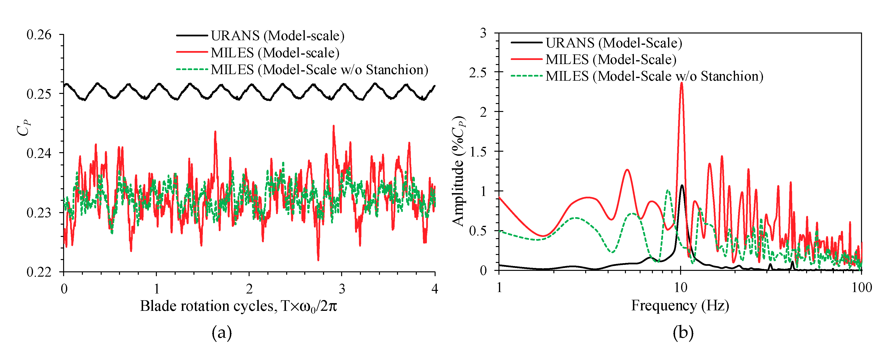
5.1. Thrust and Power Predictions

The mean CP and CT predictions, including contributions from the pressure and viscous components, are reported in Table 1. For CT, Ansys/Fluent predictions compare within 1% of the experimental data, whereas the OpenFOAM under predicts the values by about 7.5%. For CP, Ansys/Fluent is over predictive, whereas OpenFOAM is under predictive, and both show similar error levels of approximately 10 to 15%. The best results are obtained using MILES for which the results agree within 3.5% of the experimental data. This is surprising, as MILES is not expected to accurately predict the blade boundary layer. An inspection of the pressure and viscous components shows that CT is primarily (about 98–99%) due to the surface pressure distribution. However, both viscous and pressure components affect the power predictions. The former is about one-third of the latter and reduces the power production. The differences in CP predictions, either between the solvers or turbulence models, is due to the pressure component.
Results show C P , F ~   0.1 for both solvers and turbulence model. Wilson et al. [48] evaluated viscous correction for wind turbine for power production by comparing potential flow predictions and experimental data. The study showed that varied from C P , F   ~   0.1 to 0.2. The present results show a similar range. On the other hand, a recent study using the boundary element method by Salvatore et al. [49] reported that viscous forces significantly affect TST performance characteristics for λ < 3, i.e., when the flow encounters massive flow separation and stall, but does not show significant effects for λ ≥ 5. Mason-Jones et al. [8] analyzed the experimentally measured performance characteristics of model (D = 0.5 m) and full-scale (D = 10 m and 30 m) TSTs for which the ReD varied from 3 × 10⁴ to 107. The analysis of the full-scale experimental data (ReD = 3 × 10⁶ to 107) showed that TST performance is Re independent for the entire λ range (0–7.4), whereas the peak performance characteristics (at λ = 3.64) achieved Re independence only above a critical ReD,c > 3 × 10⁵. This suggests that changes in viscous stress for Re > ReD,c are negligible.
The distributions of pressure and shear stress (τw) magnitude on the blade surface are analyzed to understand their roles in thrust and power prediction. Contours of pressure coefficient and τw normalized by 1 / 2 ρ U 0 2 are shown in Figure 5, and their profiles at selected cross-section (normalized by relative velocity) are shown in Figure 6. Only URANS results are shown in Figure 5 but results from both solvers and turbulence models are shown in Figure 6. Results show high pressure on the leading edge of the entire blade due to flow stagnation. For the top 1/3rd of the blade, higher pressure is observed towards the windward face trailing edge, and lower pressure is observed towards the leeward face in between the leading edge and the mid-chord. As shown in Figure 6, the leeward face shows higher pressure than the windward face for 80% of the chord length starting from 20% aft of the leading edge, and the differences in the windward and leeward face pressures increase from the root to the tip. The results are very similar for both solvers and turbulence models at y/D = 0.16 and 0.25 but show difference towards the tip. These pressure differences induce lift on the blade, which contributes to both power production and thrust. As demonstrated in Figure 5c, the lift contribution to the power production decreases from root to tip due to the twist of the blade, and an opposite behavior is expected for their thrust contribution. For example, the cross-section towards the tip of the blade is almost aligned with the rotation plane, thus lift contributes mainly to the thrust. Also, taking into consideration that the chord length decreases from root to tip, it can be concluded that most of the power is generated due to the pressure differences in the windward and leeward faces near the mid-span of the blade. The pressure differences between the leading and trailing edges of the blades produces drag on the blade. However, this component is expected to be small considering that the airfoil is a slender body.
The surface shear stress distribution shows high values on top outboard portion of the blade on both the windward and leeward faces. As shown in Figure 6, the stresses on the leeward (high speed) side is consistently higher than those on the windward (low speed) side. Shear stresses act opposite to the flow direction and thus result in drag, which results in either thrust or power reduction. Considering that high stresses occur towards the tip, where the drag contributes primarily to power loss and the moment arm is large; they are expected to affect CP more than CT as obtained above. The URANS and IDDES models show similar predictions for both solvers but significant differences are observed between the solvers, mostly towards the blade tip.
In summary, the present study shows that power production is primarily due to lift caused by pressure differences on windward and leeward blade surfaces near the mid-span of the blade. Shear stresses generated on the leeward (high speed) side of the blade tips have significant contribution to power loss; thus, CP for the present flow condition, where λ ~ 1.7λP, is not expected to be Re independent. This aspect needs to be further investigated including simulations for λ values corresponding to peak power production. Furthermore, the differences between the turbulence models and solvers (which use different y+) suggest that the boundary layer and surface pressure distribution predictions are correlated. Future simulations should be performed near-wall grid resolution of y+ ~1 to avoid numerical uncertainties due to boundary layer resolution issues.
Figure 7 shows the temporal evolution of CP and its fast Fourier transform predicted using different turbulence model for TST w/and w/o stanchion. For the TST w/o stanchion, CT and CP time histories predicted by URANS and IDDES show steady values. MILES predicts unsteady values with fluctuation amplitudes that are ~3% of the mean; however, the fluctuations do not have a dominant frequency. The TST w/stanchion shows unsteady CT and CP for all turbulence models. For URANS and IDDES, the unsteadiness is primarily large-scale with a single dominant frequency f = 10 Hz and amplitude of approximately 1.2% of the mean. MILES predictions show large fluctuation with a wide spectral content. The dominant peak frequency is f ~10 Hz, i.e., the same as the URANS and IDDES predictions, and peak amplitudes is ~2.5% of the mean. The dominant frequency is close to NB × ω0/2π, where NB is the number of blades; thus, the unsteady behavior is attributed to the disruption of the flow each time a blade passes in front of the stanchion. Such blade-tower interaction is well documented in the literature [18,50].

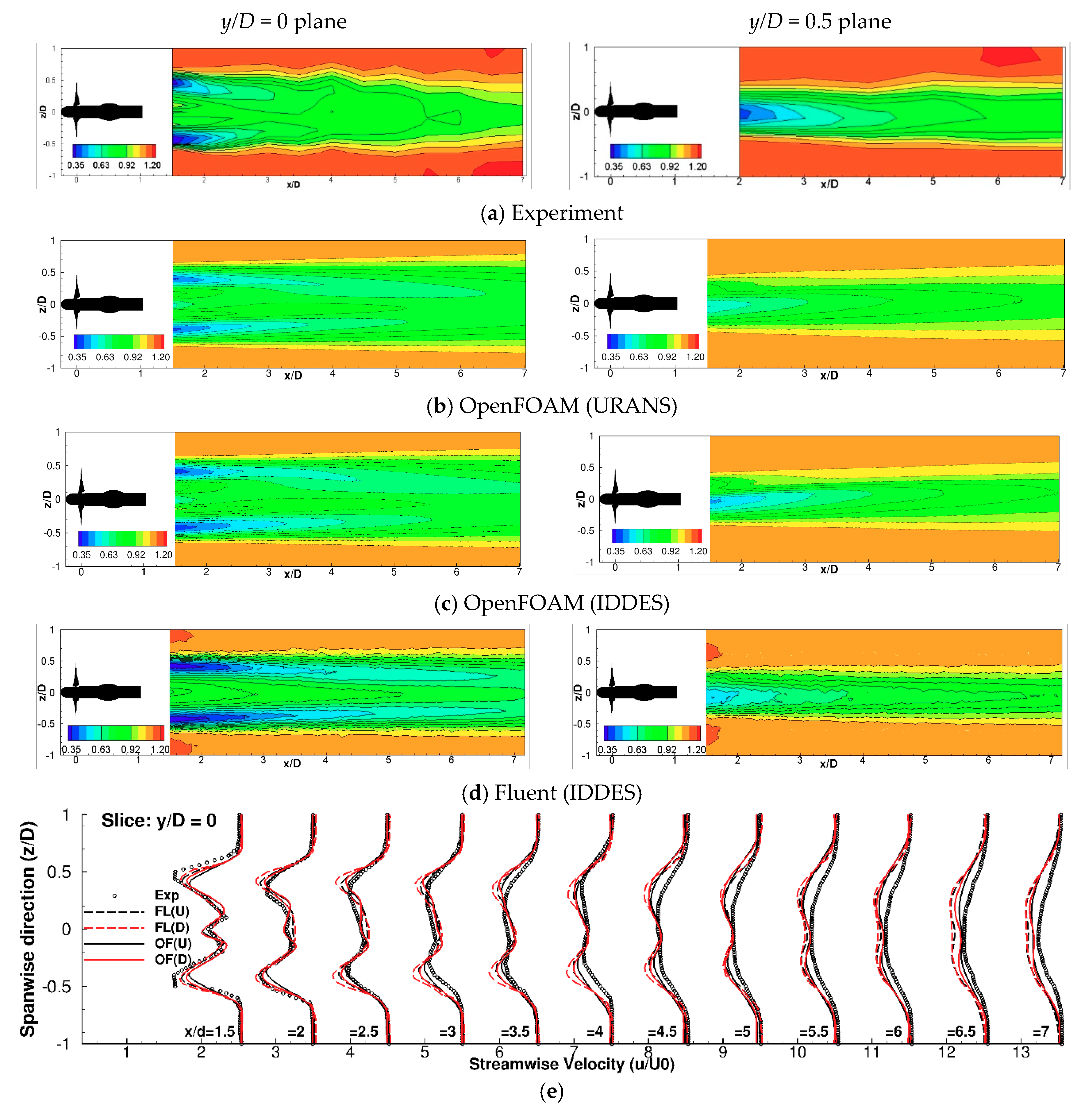
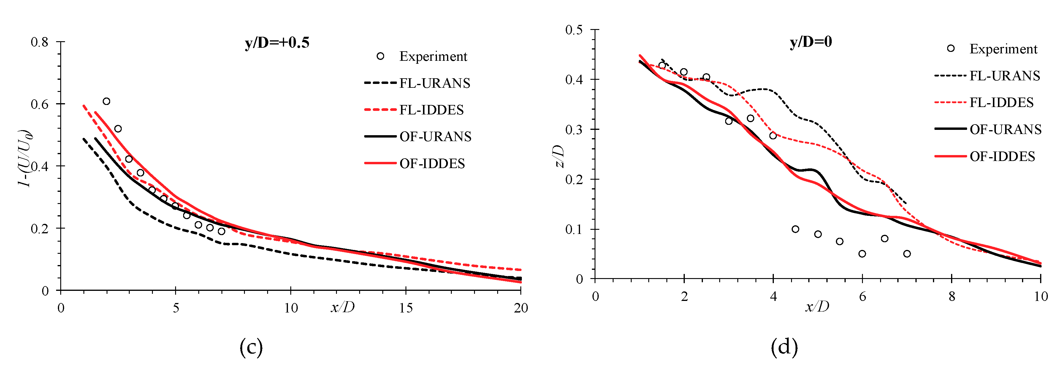
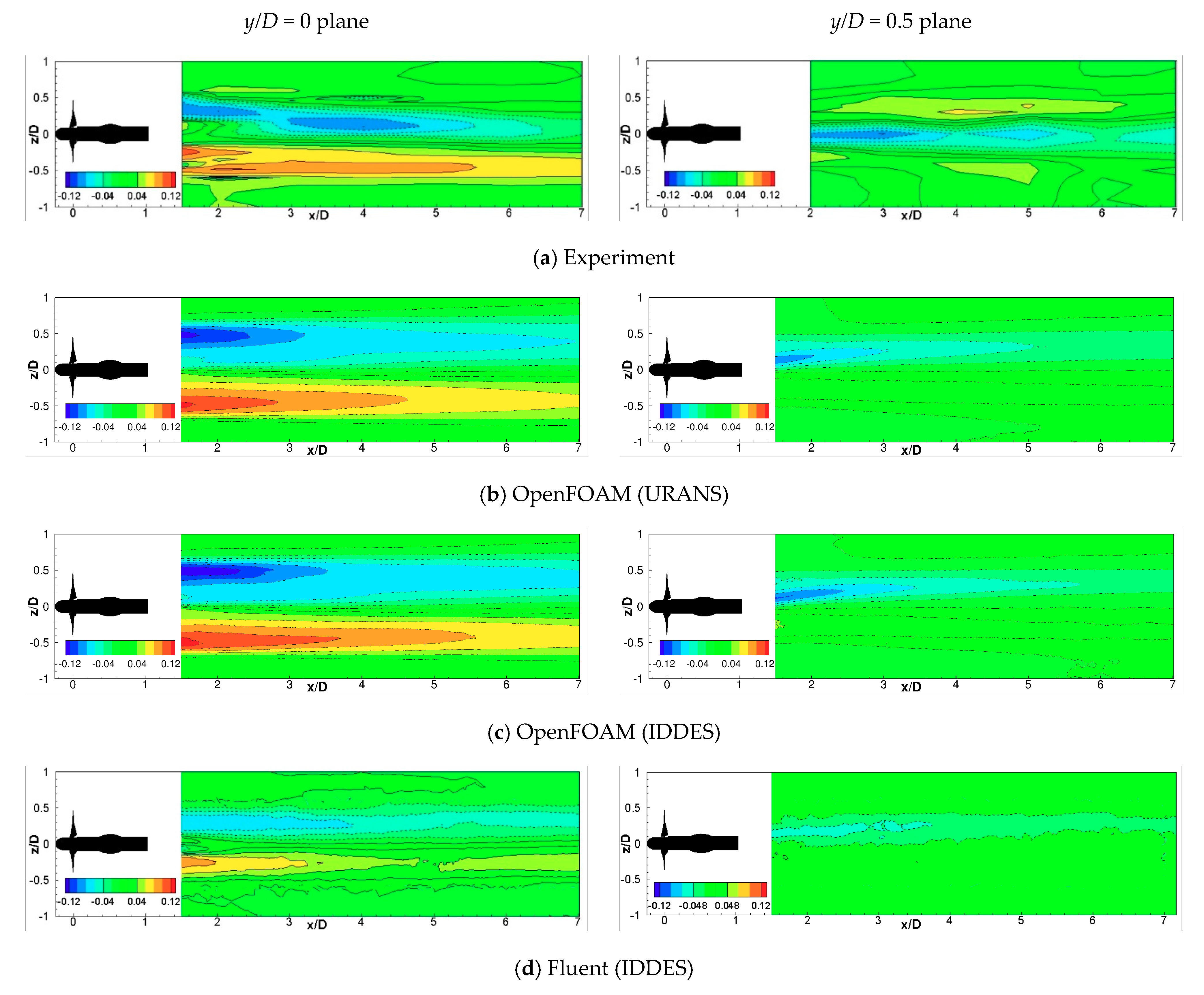
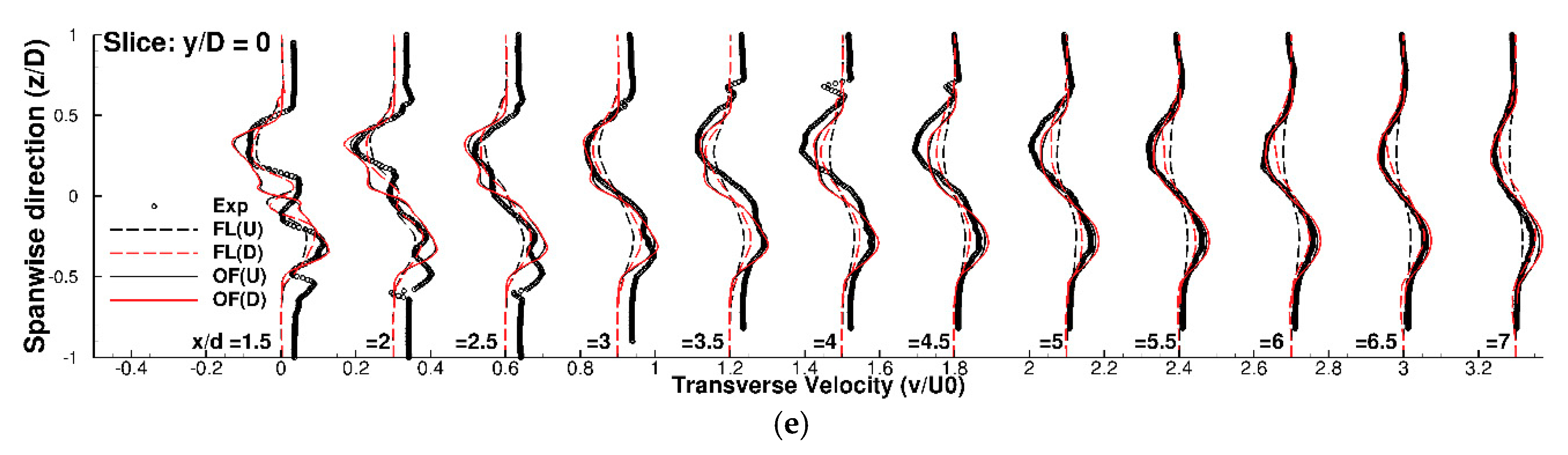
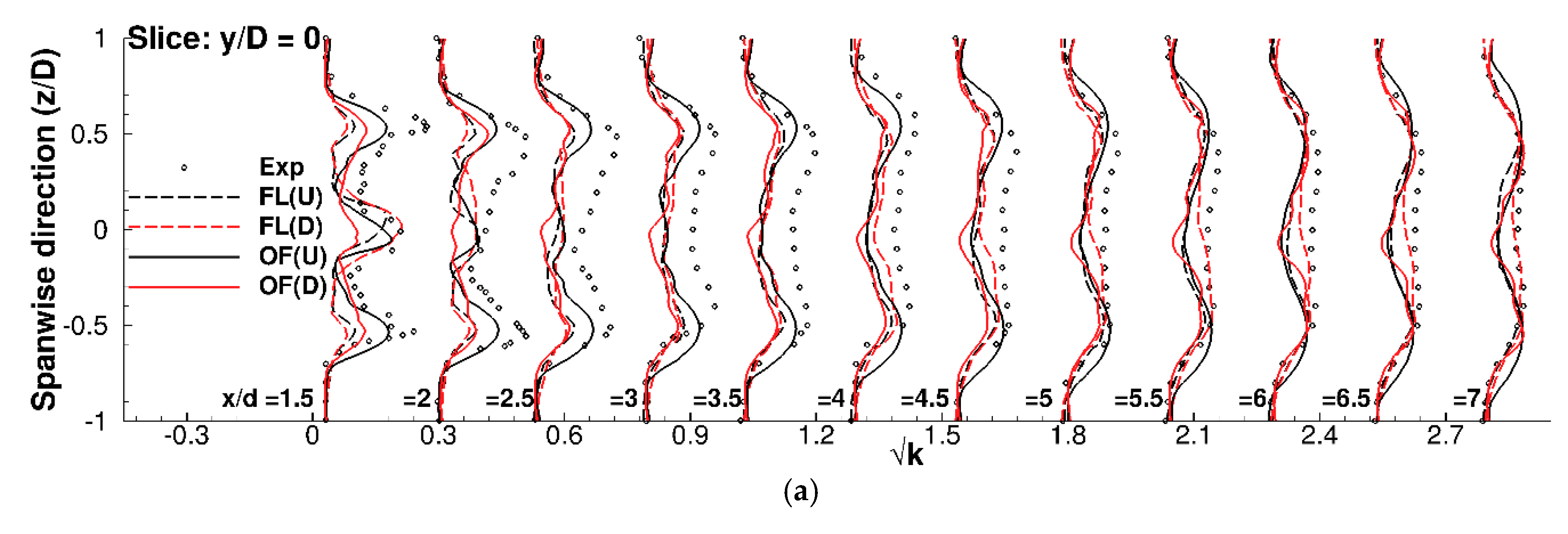
5.2. Mean and Turbulent Wake Validation

The mean streamwise velocity contours observed in the experiment in the y/D = 0 and y/D = 0.5 planes are shown in Figure 8a. The wake deficit (1-u/U0) profiles in the y/D = 0 plane are also shown in Figure 8e. The data shows that in the y/D = 0 plane, the peak mean wake deficit is 71%U0 at z/D ~± 0.47, which is directly downstream of the blade tips. The deficit peak moves towards the axis and reaches the center by x/D = 5.5 to 6, where the deficit is approximately 16%U0. The deficit contours in the planes at y/D = ± 0.25 are qualitatively similar to those in the plane at y/D = 0 except that the peak occurs at z/D ~± 0.32, slightly inward of the tip location on the plane at z/D ~± 0.43. The mean deficit behind the blade tips in the planes at y/D = ± 0.5 show a peak value around z/D~0, which decreases gradually in the downstream direction. The stanchion side planes at y/D = 0.25 and 0.5 show 2% and 6% higher deficits throughout the intermediate wake, respectively, compared to those in the center plane at y/D = 0. On the other hand, the non-stanchion side planes at y/D = −0.25 and −0.5 show 5% and 14% lower wake deficits, respectively.
Instantaneous vortical structures obtained in the IDDES solutions are shown in Figure 9a,b. Results show the generation of tip vortices, which are torus-shaped vortex, these vortices rotate around the turbine axis and are advected downstream. The vortical structures grow in diameter slowly as they advance in the streamwise direction. Note that the tip vortex ring is not visible once it interacts with the stanchion. However, its effect is evident in the transverse wake velocity distribution in Figure 9e, which shows alternate positive and negative values due to the passage of the tip vortices (which have counterclockwise vorticity ωz). Notice that the transverse velocity shows that the large-scale structures grow (in both size and strength) in the far wake region. The growth of the structures is expected due to diffusion of the vortices, but the strengthening is probably due to the underprediction of turbulence as discussed below. The tip vortices show a spacing of 0.22 D in the wake as shown in Figure 9c. The vortex ring spacing is 25% lower than 2 π U 0 / ( N B ω 0 ) = 0.29 , i.e., the vortex ring is advected at a slower velocity than the free-stream velocity. This is expected as the flow velocity behind the turbine is slower than the undisturbed upstream flow. The predictions also show spiral vortex rings emerging from the root of the blades. The root vortices show strong interaction with the turbine-shaft boundary layer and the flow separation behind the shaft. The vortex ring shrinks in diameter and dissipates much quicker than the tip vortices. The velocity deficit behind the blade is primarily caused by the spiral vortex ring emerging from the blade tips. As shown in Figure 9d, the peak deficit region grows downstream primarily towards the turbine axis, and eventually merges near the axis consistent with the experimental data. Note that the deficit recovery is faster above the turbine center-plane (y/D > 0) than below the center-plane (y/D < 0), because of additional turbulence generated from the stanchion.
The trajectory of the peak wake deficit location in the plane at y/D = 0 is shown in Figure 10a. Experiments show that the peak deficit moves inward towards the turbine axis steadily up to x/D ≤ 4 followed by a rapid inward shift further downstream. CFD predicts that the peak deficit moves towards the axis steadily and reaches the axis around x/D = 8. The CFD predictions overall underpredict the wake diffusion towards the turbine axis for x/D > 4. OpenFOAM performs somewhat better than Ansys/Fluent, and for both solvers, URANS performs better than IDDES.
The CFD wake deficit predictions are qualitatively consistent with the experimental data, as shown in Figure 8b–e. To quantitatively validate CFD predictions, the peak wake deficits in the planes at y/D = 0, ± 0.25 and ± 0.5 are compared with the experimental data in Figure 10, and averaged errors over the entire intermediate plane and all the planes are summarized in Table 1. The OpenFOAM wake deficit predictions compare within 10% of the experimental data, whereas the Ansys/Fluent predictions show an average error of 24%. The prediction errors are smaller on the stanchion side and larger on the non-stanchion side, e.g., the OpenFOAM predictions have averaged errors of E~12.2%, 10.1% and 8.2% for y/D = −0.5, 0, 0.5, respectively. Among the turbulence models URANS performs better than IDDES, e.g., the OpenFOAM predictions have averaged error of E ~7.5% and 13% for URANS and IDDES, respectively.
The experimental data for mean transverse velocities (v) at y/D = 0 plane in Figure 11 shows negative and positive values for positive and negative z/D, respectively. The peak |v|~ 0.12U0 is observed at x/D ~1.5 and decreases downstream. The peak location shows asymmetry and the profile tends to shift towards the negative z/D direction. The transverse velocity on the stanchion side (y/D = 0.5) shows a minimum around z/D ~ 0 with peak |v|~ 0.1U0 whereas they do not show any well-defined structure on the non-stanchion side. CFD predictions show the negative and positive v contours consistent with the experiment. In the intermediate wake the tip vortices start to gradually lose their shape, the mixing between the free stream and core flow happens and the turbulence begins to decay much later. Analysis of the instantaneous solution shows that the antisymmetric velocity pattern is predicted due to the counterclockwise swirl imparted by clockwise rotating turbine in the wake. The peak |v| is obtained around z/D ~ 0.3, which is in between the blade tip and the root. The transverse velocity profile in the wake are compared in Figure 11e. Note that the experimental data was shifted by z/D = 0.18 for x/D ≥ 3 to adjust for the asymmetry. The OpenFOAM predictions show much better agreement with the experimental data compared to Ansys/Fluent, and no significant difference were observed between URANS and IDDES predictions. In Ansys/Fluent simulations, the IDDES predictions were somewhat better than those of URANS, and MILES predictions were similar to those of IDDES.
The experimental data for mean spanwise velocity shows mostly small velocities with peak values |w|< 0.05U0 (figure not shown). The spanwise velocity does not show any well-defined structure. The CFD predictions also show almost negligible spanwise velocity with |w| < 0.1 U0.
The intermediate wake TKE profiles predicted by the simulations at y/D = 0 plane is compared with experiment data in Figure 12. The experimental data shows large TKE values close to the blade tips around z/D = 0.55 for x/D ≤ 2. The peak TKE moves slightly towards the axis, and an almost uniform TKE is observed at x/D = 4.5. The peak TKE value decreases with x/D, where the rate of decay is much higher close to the turbine. The data also shows high TKE towards the axis at x/D = 1.5, which decays rapidly and is not observed at x/D = 2.5. Although not shown here, the Reynolds stress invariant map in the intermediate wake region illustrates that the turbulence in the near wake tip-vortex region is strongly anisotropic and is primarily two-component turbulence, dominated by u’ and w’. The turbulence is mostly isotropic in the intermediate wake, where u’ account of is about 30–40% of the TKE. The simulations perform well and predict high TKE around z/D = 0, which is due to the flow separation from the hub. In the near wake (x/D ≤ 2.5) tip vortex region, OpenFOAM URANS performs the best among the simulations. IDDES underpredicts the high TKE in the tip vortex region, where LES is expected to be active. The resolved and modeled TKE components show that the resolved component is absent in the Ansys/Fluent simulations. In the OpenFOAM simulations, the resolved component dominates the modeled component in this region, but the TKE is significantly underpredicted when compared with the experimental data. In both solvers, resolved turbulent fluctuations are dominant for x/D ≥ 4. In this region, the OpenFOAM IDDES predictions are similar to those of URANS, and are lower than the experiments. The Ansys/Fluent IDDES predictions compare quite well with the experimental data for x/D ≥ 5.5.

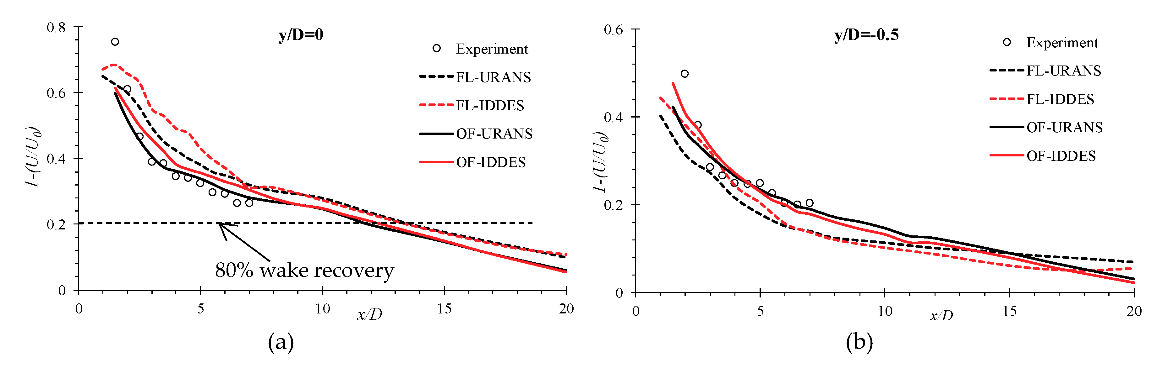
5.3. Far Wake Prediction

The far wake profiles in the plane at y/D = 0 and streamwise locations x/D = 8 to 20 predicted for λ = 3.64 (taken from Salunkhe [39]) and λ = 6.15 were analyzed to evaluate the far-wake recovery characteristics and are shown in Figure 13. The amplitude in the figure is the normalized wake deficit δ U = ( 1 u ) / ( 1 u z = 0 ) , where u z = 0 is the streamwise velocity at centerline z = 0. The half-wake width (δH) was obtained by normalizing the abscissa using the z/D width of the deficit profile at 0.75 δ U , i.e., δH = ± 0.25 occurs at 0.75 δ U . Results for both λ values show very good self-similarity and compare well with a Gaussian distribution. Both the wake deficit amplitude and width show a linear variation with x/D, and their slopes are very similar for both values of λ. The averaged wake growth and amplitude decay rates are approximately 0.03 D and 0.0185 U0/D respectively. Bastankhan and Porte-Agel [51] analyzed high resolution measurements and LES results wind turbines and reported that the wake growth rate lies within the range 0.023 to 0.055 D. The present results lie within this range.

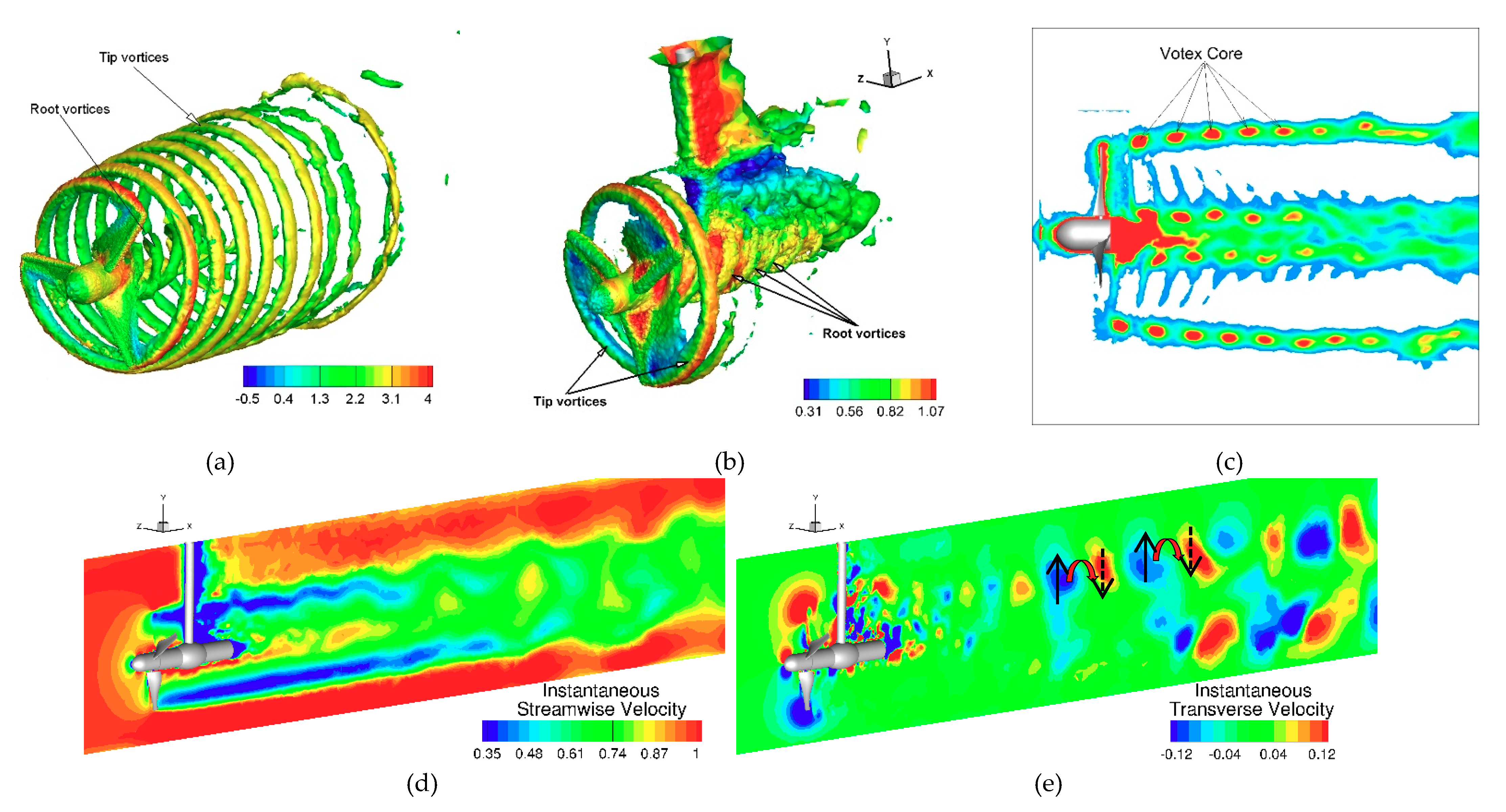
6. Discussions: Wake Recovery Mechanism

A synthesis of the CFD predictions (including those presented in Salunkhe [39]) and experimental data reveals that the near wake region is dominated by large-scale vortical structures generated from the tip of the turbine blades. The tip vortices produce an annular inverted jet with two shear layers, one developing inward towards the turbine axis and other developing outward of the blade tip region. The outer shear layer growth is primarily due to inflow turbulence, while the inner shear layer growth is due to turbulence generated by the turbine. Turbulence generated by the turbine consists of two-component, streamwise and cross-flow fluctuations, and the latter is primarily responsible for wake diffusion towards the center. The turbulence slowly evolves into 3D isotropic turbulence in the far-wake but is highly anisotropic in the intermediate wake region.
The near wake and intermediate wake recovery are significantly affected by the value of λ (or power production) and the stanchion. The wake deficit is related to the power production, i.e., the higher the power production, the higher the wake deficit. The rate of deficit recovery is found to be independent of power production (or λ); thus, the recovery length is directly related to the power production. The stanchion induces additional turbulence, which enhances the diffusion of the peak wake deficit towards the axis resulting in faster wake recovery. The far-wake starts at x/D = 8, and the wake deficit shows self-similarity with a Gaussian deficit profile. The wake recovery is found to be independent of both power production and the stanchion.

7. Conclusions and Future Work

Simulations were performed for a model-scale tidal stream turbine for λ = 6.15, which is 1.7 times higher than the value of λ needed for peak power production, using Ansys/Fluent and OpenFOAM with URANS and IDDES turbulence models on manually refined and solution-adapted grids consisting of up to 11 M cells. The turbine performance and intermediate wake predictions are validated using experimental data and results are analyzed to develop an understanding of the wake recovery mechanism.
The solvers provided mixed results, both under- and over-predictions for thrust and power, with the errors being limited to around 10%. The thrust predictions were dominated by the pressure distribution on the blades and were found to be scale independent. The power production was primarily due to pressure generated lift near the mid-span of the blade. The shear stress is generated mostly on the leeward (high speed) side of the blade tips and results in around a 30% power reduction. Thus, turbulence models and near-wall grid resolution on the blades are important for accurate power prediction, especially for operations at off-design conditions.
The flow in the near wake region (x/D < 2) is predicted well, however the turbulent kinetic energy is significantly underpredicted. In this region, OpenFOAM performs better than Ansys/Fluent, and URANS better than IDDES. IDDES fails to trigger resolved turbulence due to the modeled stress depletion issue, which has been well documented in the literature for both canonical cases [52] and engineering applications [53]. The wake growth in the intermediate wake region (i.e., up to x/D = 4) is underpredicted by both URANS and IDDES. In the former, the underprediction is likely due to their inability to predict turbulence anisotropy, and for the latter it is due to lack of resolved turbulence. Further downstream (i.e., x/D > 4), IDDES predicts resolved turbulence and performs better than URANS for both the mean wake and turbulent kinetic energy predictions.
Overall, the predictions reported in this study are reasonable, but can be significantly improved. The study shows that fine grid resolutions are essential for accurate prediction of large-scale vortical structures in the near wake region, and accurate turbulence predictions are essential for improved intermediate wake predictions which involve anisotropic turbulence in the tip-vortex shear layer. Hybrid RANS/LES models are preferable over URANS, as they rely less on modeling. Most commonly used DES models (and its variants) suffer from modeled stress depletion issue; thus, other advanced models such as dynamic hybrid RANS/LES [52] should be investigated. The errors in the predictions could also be due to neglect of free-surface effects and will be investigated in future studies. The differences in the boundaries in the transverse direction (i.e., free-surface on the top and wall on the bottom) can result in flow asymmetry in the transverse direction, and perhaps also in the spanwise and streamwise directions [54]. However, the experimental data shows significant, unanticipated flow asymmetry in the spanwise direction, which could explain some of the observed differences between the experimental data and predicted results. Furthermore, the experiments were performed in a flume with blockage ratio of approximately 16%. The performance curve and wake are expected to be significantly different from full-scale applications. An experimental campaign is underway to obtain additional wake validation data in a wave basin. Future study will also focus on investigation of the effects of TI, λ and Re on the wake recovery. For the former, simulations should focus on specification of inflow turbulence anisotropy consistent with the experiments, and the grid should be designed such that specified inlet turbulence is advected accurately up to the turbine.

Author Contributions

Conceptualization, S.B., D.T., D.O. and T.O.; methodology, S.B.; software, S.S. and O.E.F.; validation, S.S., O.E.F., S.B. and A.M.-J.; formal analysis, S.B. and D.T.; investigation, S.B., D.T., T.O. and A.M.-J.; resources, D.T., D.O. and T.O.; data curation, T.O. and A.M.-J.; writing—original draft preparation, S.S. and S.B.; writing—review and editing, S.S., O.E.F., S.B., D.T. and T.O.; visualization, S.S. and O.E.F.; supervision, D.T. and T.O.; project administration, D.T. and T.O.; funding acquisition, D.T., T.O., D.O. and A.M.-J.”

Funding

EPSRC EP/N020782/1 under the Supergen Marine Grand Challenge program.

Acknowledgments

This effort was partially supported by the Center for Advanced Vehicular Systems, Mississippi State University. All simulations were performed on Talon HPC system at High Performance computing Collaboratory, Mississippi State University. The contribution of Robert Poole, School of Engineering at the University of Liverpool, who provided detailed experimental data, is also gratefully acknowledged. The authors also acknowledge the financial support of EPSRC EP/N020782/1 under the Supergen Marine Grand Challenge program.

Conflicts of Interest

The authors declare no conflict of interest.

References

  1. IPCC. 2011: Summary for Policymakers. In IPCC Special Report on Renewable Energy Sources and Climate Change Mitigation; Edenhofer, O., Pichs-Madruga, R., Sokona, Y., Seyboth, K., Matschoss, P., Kadner, S., Zwickel, T., Eickemeier, P., Hansen, G., Schlömer, S., et al., Eds.; Cambridge University Press: Cambridge, UK; New York, NY, USA, 2011. [Google Scholar]
  2. Tedds, S.C.; Owen, I.; Poole, R.J. Near wake characteristics of a model horizontal axis tidal stream turbine. Renew. Energy 2014, 63, 222–235. [Google Scholar] [CrossRef]
  3. Egarr, D.A.; O’Doherty, T.; Morris, T.; Ayre, R.G. Feasibility study using computational fluid dynamics for the use of a turbine for extracting energy from the tide. In Proceedings of the 15th Australasian Fluid Mechanics Conference, The University of Sydney, Sydney, Australia, 13–17 December 2004. [Google Scholar]
  4. Churchfield, M.J.; Li, Y.; Moriarty, P.J. A large-eddy simulation study of wake propagation and power production in an array of tidal-current turbines. Philos. Trans. R. Soc. A 2013, 371, 20120421. [Google Scholar] [CrossRef] [PubMed] [Green Version]
  5. Myers, L.W.; Bahaj, A.S. Experimental analysis of the flow field around horizontal axis tidal turbines by use of scale mesh disk rotor simulators. Ocean Eng. 2010, 37, 218–227. [Google Scholar] [CrossRef]
  6. Maganga, F.; Germain, G.; King, J.; Pinon, G.; Rivoalen, E. Experimental characterization of flow effects on marine current turbine behaviour and on its wake properties. Renew. Power Gener. IET 2010, 4, 498–509. [Google Scholar] [CrossRef]
  7. Sørensen, J.N.; Shen, W. Numerical modeling of wind turbine wakes. J. Fluids Eng. 2002, 124, 393–402. [Google Scholar] [CrossRef]
  8. Mason-Jones, A.; O’Doherty, D.M.; Morris, C.E.; O’Doherty, T.; Byrne, C.B.; Prickett, P.W.; Grosvenor, R.I.; Owen, I.; Tedds, S.; Poole, R.J. Non-dimensional scaling of tidal stream turbines. Energy 2012, 44, 820–829. [Google Scholar] [CrossRef]
  9. Vermeer, L.J.; Sørensen, J.N.; Crespo, A. Wind turbine wake aerodynamics. Prog. Aerosp. Sci. 2003, 39, 467–510. [Google Scholar] [CrossRef]
  10. Shen, W.; Mikkelsen, R.; Sørensen, J.N.; Bak, C. Tip loss corrections for wind turbine computations. Wind Energy 2005, 8, 457–475. [Google Scholar] [CrossRef]
  11. Contreras, L.T.; Lopez, O.D.; Lain, S. Computational Fluid Dynamics Modelling and Simulation of an Inclined Horizontal Axis Hydrokinetic Turbine. Energies 2018, 11, 3151. [Google Scholar] [CrossRef]
  12. Brand, A.J.; Peinke, J.; Mann, J. Turbulence and wind turbines. J. Phys. Conf. Ser. 2011, 318, 072005. [Google Scholar] [CrossRef]
  13. Ainslie, J.F. Calculating the field in the wake of wind turbines. J. Wind Eng. Ind. Aerodyn. 1988, 27, 213–224. [Google Scholar] [CrossRef]
  14. Crespo, A.; Hernandez, J.; Frega, E.; Andreu, C. Experimental validation of the UPM computer code to calculate wind turbine wakes and comparison with other models. J. Wind Eng. Ind. Aerodyn. 1988, 27, 77–88. [Google Scholar] [CrossRef]
  15. Magnusson, M.; Smedman, A.S. Air flow behind wind turbines. J. Wind Eng. Ind. Aerodyn. 1999, 80, 169–189. [Google Scholar] [CrossRef]
  16. Larsen, G.; Madsen, H.; Thomsen, K.; Larsen, T. Wake meandering: A pragmatic approach. Wind Energy 2010, 11, 377–395. [Google Scholar] [CrossRef]
  17. Elvira, R.G.; Crespo, A.; Migoya, E.; Manuel, F.; Hernandez, J. Anisotropy of Turbulence in Wind Turbine Wakes. J. Wind Eng. Ind. Aerod. 2005, 93, 797–814. [Google Scholar] [CrossRef]
  18. Afgan, I.; McNaughton, J.; Rolfo, S.; Apsley, D.; Stallard, T.; Stansby, P. Turbulent flow and loading on a tidal stream turbine by LES and RANS. Int. J. Heat Fluid Flow 2013, 43, 96–108. [Google Scholar] [CrossRef]
  19. Ahmed, U.; Apsley, D.D.; Afgan, I.; Stallard, T.; Stansby, P.K. Fluctuating loads on a tidal turbine due to velocity shear and turbulence: Comparison of CFD with field data. Renew. Energy 2017, 112, 235–246. [Google Scholar] [CrossRef] [Green Version]
  20. Shen, W.Z.; Zhang, J.; Sørensen, J.N. The actuator surface model: A new Navier—Stokes based model for rotor computations. J. Sol. Energy Eng. 2009, 131, 011002. [Google Scholar] [CrossRef]
  21. Batten, W.M.J.; Harrison, M.E.; Bahaj, A.S. Accuracy of the actuator disc-RANS approach for predicting the performance and wake of tidal turbines. Philos. Trans. R. Soc. A 2013, 371, 20120293. [Google Scholar] [CrossRef] [PubMed] [Green Version]
  22. Johansen, J.; Sørensen, N.N.; Michelsen, J.A.; Schreck, S. Detached-eddy simulation of flow around the NREL phase VI blade. Wind Energy 2002, 5, 185–197. [Google Scholar] [CrossRef]
  23. Blackmore, T.; Batten, W.; Bahaj, A.S. Turbulence generation and its effect in LES approximations of tidal turbines. In Proceedings of the 10th European Wave and Tidal Energy Conference, Aalborg, Denmark, 2–5 September 2013. [Google Scholar]
  24. Bowman, J.; Bhushan, S.; Thompson, D.; O’Doherty, D.; O’Doherty, T.; Mason-Jones, A. A Physics-Based Actuator Disk Model for Hydrokinetic Turbines. In Proceedings of the 2018 Fluid Dynamics Conference, AIAA AVIATION Forum, (AIAA 2018–3227), Atlanta, Georgia, 25–29 June 2018. [Google Scholar]
  25. Troldborg, N.; Sørensen, J.N.; Mikkelsen, R. Actuator line simulation of wake of wind turbine operating in turbulent inflow. J. Phys. Conf. Ser. 2007, 75, 012063. [Google Scholar] [CrossRef]
  26. Mason-Jones, A.; O’Doherty, D.M.; Morris, C.E.; O’Doherty, T. Influence of a velocity profile & support structure on tidal stream turbine performance. Renew. Energy 2013, 52, 23–30. [Google Scholar]
  27. Frost, C.; Morris, C.E.; Mason-Jones, A.; O’Doherty, D.M.; O’Doherty, T. Effects of tidal directionality on tidal turbine characteristics. J. Renew. Energy 2015, 78, 609–620. [Google Scholar] [CrossRef]
  28. Zahle, F.; Sørensen, N.N.; Johansen, J. Wind turbine rotor–tower interaction using an incompressible overset grid method. Wind Energy 2009, 12, 594–619. [Google Scholar] [CrossRef]
  29. Li, Y.; Castro, A.M.; Sinokrot, T.; Prescott, W.; Carrica, P.M. Coupled multi-body dynamics and CFD for wind turbine simulation including explicit wind turbulence. Renew. Energy 2015, 76, 338–361. [Google Scholar] [CrossRef]
  30. Marchevsky, I.K.; Puzikova, V.V. Numerical Simulation of Wind Turbine Rotors Autorotation by Using the Modified LS-STAG Immersed Boundary Method. Int. J. Rotating Mach. 2017, 2017, 6418108. [Google Scholar] [CrossRef]
  31. Ouro, P.; Stoesser, T. An immersed boundary-based large-eddy simulation approach to predict the performance of vertical axis tidal turbines. Comput. Fluids 2017, 152, 74–87. [Google Scholar] [CrossRef] [Green Version]
  32. Bhushan, S.; Carrica, P.; Yang, J.; Stern, F. Scalability and Validation Study for Large Scale Surface Combatant Computations Using CFDShip-Iowa. Int. J. High-Perform. Comput. Appl. 2011, 25, 466–487. [Google Scholar] [CrossRef]
  33. Kasmi, A.; Masson, C. An extended k-ε model for turbulent flow through horizontal axis wind turbines. J. Wind Eng. Ind. Aerodyn. 2008, 96, 103–122. [Google Scholar] [CrossRef]
  34. Cabezon, D.; Migoya, E.; Crespo, A. Comparison of turbulence models for the Computational fluid dynamics simulation of wind turbine wakes in the atmospheric boundary layer. Wind Energy 2011, 14, 909–921. [Google Scholar] [CrossRef]
  35. O’Brien, J.M.; Young, T.M.; Early, J.M.; Griffin, P.C. An assessment of commercial CFD turbulence models for near wake HAWT modelling. J. Wind Eng. Ind. Aerodyn. 2018, 176, 32–53. [Google Scholar] [CrossRef] [Green Version]
  36. Archera, C.L.; Vasel-Be-Hagha, A.; Yana, C.; Wua, S.; Yang Pana, Y.; Brodiea, J.F.; Maguire, A.E. Review and evaluation of wake loss models for wind energy applications. Appl. Energy 2018, 226, 1187–1207. [Google Scholar] [CrossRef]
  37. FLUENT 6.3; User Guide FLUENT 6.3; FLUENT Inc.: Lebanon, NH, USA, 2006.
  38. Jasak, H.; Jemcov, A.; Tukovic, Z. Openfoam: A C++ library for complex physics simulations. In International Workshop on Coupled Methods in Numerical Dynamics; IUC Dubrovnik: Dubrovnik, Croatia, 2007. [Google Scholar]
  39. Salunkhe, S. Model—and Full-Scale Predictions of Hydrokinetic Turbulent Wake, Including Model-Scale Validation. Master’s Thesis, Mississippi State University, Starkville, MS, USA, 2016. [Google Scholar]
  40. Menter, F.R. Two-equation eddy-viscosity turbulence models for engineering applications. AIAA J. 1994, 32, 1598–1605. [Google Scholar] [CrossRef] [Green Version]
  41. Spalart, P.R. Detached-eddy simulation. Annu. Rev. Fluid Mech. 2009, 41, 181–202. [Google Scholar] [CrossRef]
  42. Grinstein, F.F.; Fureby, C. On Monotonically Integrated Large Eddy Simulation of Turbulent Flows Based on FCT Algorithms. In Flux-Corrected Transport. Scientific Computation; Kuzmin, D., Löhner, R., Turek, S., Eds.; Springer: Berlin/Heidelberg, Germany, 2005. [Google Scholar]
  43. Adedoyin, A.A.; Walters, D.K.; Bhushan, S. Evaluation of turbulence model and numerical scheme combinations for practical Finite-volume Large Eddy Simulations. Eng. Appl. Comput. Fluid Mech. 2015, 9, 324–342. [Google Scholar]
  44. Robertson, E.; Choudhury, V.; Bhushan, S.; Walters, D.K. Validation of OpenFOAM Numerical Methods and Turbulence Models for Incompressible Bluff Body Flows. Comput. Fluids 2015, 123, 122–145. [Google Scholar] [CrossRef]
  45. Morris, C. Influence of Solidity on the Performance, Swirl Characteristics, Wake Recovery and Blade Deflection of a Horizontal Axis Tidal Turbine. Ph.D. Thesis, Cardiff University, Cardiff, Wales, 2014. [Google Scholar]
  46. Morris, C.E.; O’Doherty, D.M.; Mason-Jones, A.; O’Doherty, T. Evaluation of the swirl characteristics of a tidal stream turbine wake. Int. J. Mar. Energy 2016, 14, 198–214. [Google Scholar] [CrossRef] [Green Version]
  47. Gupta, A.K.; Lilley, D.G.; Syred, N. Swirl Flows; Energy and Engineering Science Series; Abacus Press Tunbridge Wells: Kent, UK, 1984. [Google Scholar]
  48. Wilson, R.E.; Lissaman, P.B.S.; Walker, S.N. Aerodynamic Performance of Wind Turbines; Oregon State University: Corvallis, OR, USA, 1976. [Google Scholar]
  49. Salvatore, F.; Sarichloo, Z.; Calcagni, D. Marine Turbine Hydrodynamics by a Boundary Element Method with Viscous Flow Correction. J. Mar. Sci. Eng. 2018, 6, 53. [Google Scholar] [CrossRef]
  50. Engström, S.; Ganander, H.; Lindström, L. Short Term Power Variations in the Output of Wind Turbines. DEWI Mag. 2001, 19, 27–30. [Google Scholar]
  51. Bastankhan, M.; Porte-Agel, F. A new analytical model for wind turbine wakes. Renew. Energy 2014, 70, 116–123. [Google Scholar] [CrossRef]
  52. Bhushan, S.; Walters, D.K. A dynamic hybrid RANS/LES modeling framework. Phys. Fluids 2012, 24, 015103. [Google Scholar] [CrossRef]
  53. Bhushan, S.; Yoon, H.; Stern, F.; Guilmineau, E.; Visonneau, M.; Toxopeus, S.; Simonsen, C.; Aram, S.; Kim, S.-E.; Grigoropoulos, G. Assessment of CFD for Surface Combatant 5415 at Straight Ahead and Static Drift. J. Fluids Eng. 2019, 141, 051101. [Google Scholar] [CrossRef]
  54. Bahaj, A.S.; Myers, L.E.; Rawlinson-Smith, R.I.; Thomson, M. The Effect of Boundary Proximity Upon the Wake Structure of Horizontal Axis Marine Current Turbines. J. Offshore Mech. Arct. Eng. 2012, 134, 021104. [Google Scholar] [CrossRef]
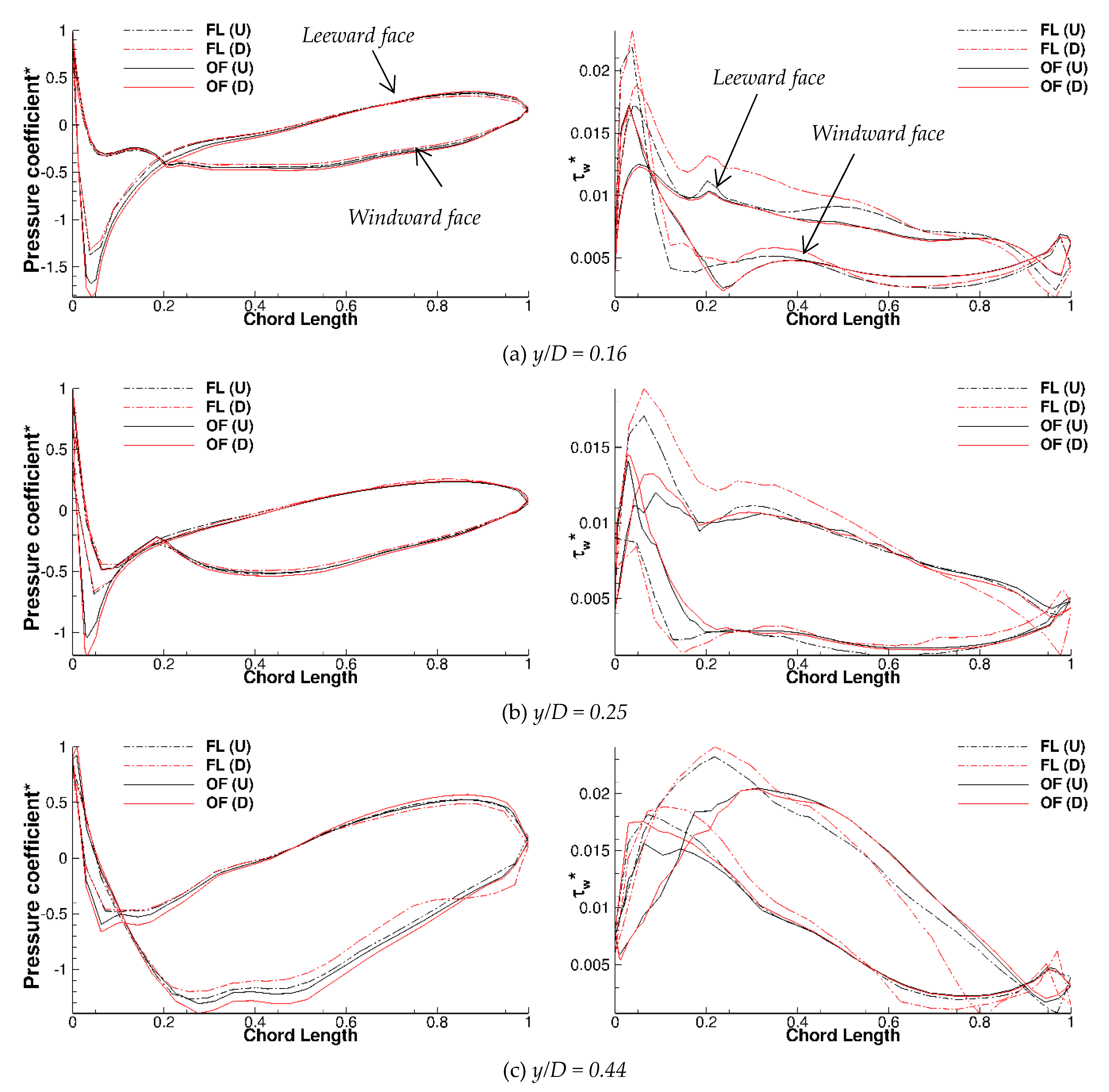
1
The experimental profiles were interpolated from the Tecplot contours plots provided by Professor Robert Poole. Thus, the symbols do not correspond the actual measurement locations.
Figure 1. (a) Computer-aided design (CAD) model of the turbine blade and support assembly. (b) Wake measurement planes y/D = ± 0.5, ± 0.25 and 0.
Jmse 07 00362 g001
Figure 2. Simulation domain and boundary conditions. Inset figure shows the rotating cylindrical domain for turbine blades and hub.
Jmse 07 00362 g002
Figure 3. Cross-sectional view of the grid at y/D = 0 plane used in the simulations. (a) The fine 8.8 M grid used in Ansys/Fluent simulations. The contour plot shows the ratio of grid scale (Δ) and turbulence length scales (ℓ). F H R L = Δ / = 1 is unsteady Reynolds averaged Navier-Stokes (URANS) region and F H R L = 0 is Large Eddy Simulation (LES) region. (b) The 11 M grid used in OpenFOAM simulations. The inset plot shows the prismatic cells in the boundary layer.
Jmse 07 00362 g003
Figure 4. Contour of velocity in the region upstream of the rotor is shown in the y = 0 plane using OpenFOAM URANS results.
Jmse 07 00362 g004
Figure 5. Blade surface (a) pressure and (b) shear stress magnitude distribution on windward face (left panel) and leeward face (right panel) obtained using URANS. (c) Flow predictions around the turbine blade close to the root (y = 0.16 D) (left panel) and close to the tip (y = 0.44 D) (right panel). The inset plot shows the plane location with respect to the turbine blade.
Jmse 07 00362 g005
Figure 6. Profile of blade surface pressure coefficient (left panel) and shear stress magnitude distribution (right panel) on windward and leeward faces obtained using Fluent and OpenFOAM unsteady Reynolds averaged Navier-Stokes (URANS) and improved delayed detached eddy simulation (IDDES) at (a) y/D = 0.16, (b) y/D = 0.25, and (c) y/D = 0.44. The coefficients are normalized by relative velocity. The abscissa is normalized by chord length at respective y/D. The y/D locations are shown in Figure 5.
Jmse 07 00362 g006
Figure 7. (a) Time history and (b) Fast Fourier Transform (FFT) of CP predictions obtained using URANS and Monotone Integrated Large Eddy Simulation (MILES) cases with and without stanchion.
Jmse 07 00362 g007
Figure 8. Mean streamwise velocity obtained from: (a) experiment [2], (b) OpenFOAM URANS, (c) OpenFOAM IDDES and (d) Ansys/Fluent IDDES. The left and right panels show the plots in y/D = 0 and 0.5 planes, respectively. (e) Wake deficit profiles1 predicted in CFD simulations in y/D = 0 plane are compared with experimental data [2].
Jmse 07 00362 g008
Figure 9. Wake flow pattern predicted by IDDES using Ansys/Fluent. Vorticity structure predicted for tidal stream turbine (TST) (a) w/o stanchion and (b) w/stanchion are shown using vorticity magnitude |ω| = 15. The vortices are colored using streamwise velocity. (c) Contour of plane normal vorticity magnitude at y/D = 0 plane for TST w/o stanchion. Instantaneous (d) streamwise (x) and (e) transverse (y) velocity contours in the wake predicted for TST w/stanchion. The sub-figure (e) shows that the alternate +ve and –ve spanwise velocities are due to passage of counter-clockwise vortices ωz.
Jmse 07 00362 g009
Figure 10. Validation URANS and IDDES wake deficit predictions from Ansys/Fluent and OpenFOAM using experimental data [2]. Variation of peak wake deficit downstream of turbine at: (a) y/D = 0, (b) y/D = -0.5 and (c) y/D = 0.5 planes. (d) Spanwise location of peak deficit at y/D = 0.
Jmse 07 00362 g010aJmse 07 00362 g010b
Figure 11. Mean transverse (y) velocity contour obtained from: (a) experiment, (b) OpenFOAM URANS, (c) OpenFOAM IDDES and (d) Ansys/Fluent IDDES. The left and right panels show the plots in y/D = 0 and 0.5 planes, respectively. (e) Transverse velocity profiles predicted in CFD simulations in y/D = 0 plane is compared with experimental data [2]. Experimental profiles for x/D ≥ 3 are shifted by z/D = 0.18, as the data shows asymmetry across z/D = 0.
Jmse 07 00362 g011aJmse 07 00362 g011b
Figure 12. (a) k profiles at different streamwise locations are compared with experimental data [2]. Contours of turbulent kinetic energy (TKE) predicted by Ansys/Fluent (left panels) and OpenFOAM (right panel) simulations at y/D = 0 plane. (b) TKE predicted by URANS. (c) Modeled component, (d) resolved component and (e) total TKE predicted by IDDES.
Jmse 07 00362 g012aJmse 07 00362 g012b
Figure 13. (a) Self-similarity in the velocity profiles compared with Gaussian curve for model-scale λ = 6.15 results, and (b) variation of the amplitude and wake width in the far wake for λ = 3.64 and 6.15 simulations. In the subfigure (b), the dotted and broken lines are the linear curve fit for λ = 3.64 and 6.15 results, respectively. λ = 3.64 results were taken from Salunkhe [36].
Jmse 07 00362 g013
Table 1. Summary of thrust and power coefficient, including contributions from pressure and viscous components, power unsteadiness, and wake recovery characteristics and prediction errors.
SolverGrid
Size
Turbulence
Model
ThrustPowerPower UnsteadinessIntermediate WakeFar Wake
CT
(%E)
CT,P
(%CT)
CT,F
(%CT)
CP
(%E)
CP,P
(%CP)
CP,F
(%CP)
Frequency (Hz)Amplitude
(%CP)
Recovery Length (D)Prediction (%E)Width Growth (D)Amplitude Decay (U0/D)
Experiment, Morris et al. [42]1.04 0.226
Fluent (F)8.8 MURANS1.042 (0.2%)1.034 (99.2%)0.013 (1.2%)0.248 (9.7%)0.342 (137.9%)‒0.094
(‒37.9%)
10.151.07%13.3324.10.031‒0.0163
IDDES1.036
(‒0.4%)
1.022 (98.6%)0.014 (1.3%)0.255 (12.8%)0.357 (140.0%)‒0.102
(‒40%)
10.191.15%13.2123.80.026‒0.0176
MILES1.052 (1.2%)1.046 (99.4%)0.008 (0.6%)0.234 (3.5%)0.296 (126.4%)‒0.063
(‒26.9%)
10.212.4%13.1025.80.028‒0.0183
OpenFOAM
(OF)
11 MURANS0.967
(‒7.0%)
0.960 (99.2%)0.0069 (0.7%)0.198
(‒12.4%)
0.303 (153%)‒0.105
(‒53.0%)
10.901.14%11.537.40.025‒0.0210
IDDES0.959
(‒7.8%)
0.952 (99.2%)0.0068 (0.6%)0.190
(‒15.9%)
0.294 (154.7%)‒0.104
(‒54.7%)
10.741.53%12.1512.90.030‒0.0204
Dominant frequency of CP time history. Corresponding to 80% U0 recovery.

