Article

Experimental and Numerical Research on the Influence of Stern Flap Mounting Angle on Double-Stepped Planing Hull Hydrodynamic Performance

1
College of Shipbuilding Engineering, Harbin Engineering University, Harbin 150001, China
2
China Ship Scientific Research Center, Wuxi 214000, China
*
Authors to whom correspondence should be addressed.
J. Mar. Sci. Eng. 2019, 7(10), 346; https://doi.org/10.3390/jmse7100346
Submission received: 30 June 2019 / Revised: 11 September 2019 / Accepted: 19 September 2019 / Published: 1 October 2019
(This article belongs to the Special Issue Ship Hydrodynamics)

Abstract

:
In the current hydrodynamic research relating to planing hulls, the stern flap and steps are generally considered to be two independent resistance reduction measures. Limited research has focused on the coupled effects of flaps and steps. Therefore, experimental and numerical simulation methods are carried out in this paper to explore the influence of the flap mounting angle coupled with the steps. A series of model towing tests were implemented for a double-stepped planing hull with 2°, 3° and 4.5° flap angles. The test results show that, as the mounting angle increased, the low speed resistance performance was improved and the porpoising critical speed was delayed, with a slight resistance cost. Based on the tests, a numerical simulation method was established with volume Froude numbers ranging from 0.88 to 5.20. The simulated hull flow field showed good agreement with the testing data. The simulation results suggest a cavity induces the negative pressure after the steps; the cavity core region is the air phase, and this expands with the air–water mixture flow. The cavity also causes wetted surface reduction and pressure distribution changes. Finally, comparisons of cavities after-steps and load coefficients of different planing surfaces among models were considered. Numerical results analysis gave distinct interpretations for the experimental phenomenon of porpoising critical speed increasing with a slight resistance increment.

1. Introduction

The stern flap, also known as the stern baffle, is always shaped as a flat plate with a high aspect ratio, fixed or angle adjustable, and attached to the rear of a high speed transom stern hull. During the navigation process, the hydrodynamic lift generated by the stern flap can affect the motion attitude of the hull, to a certain extent [1]. As a result, the pressure distribution at the hull bottom and the wave-making property of the wake field are changed, while the resistance performance is also improved [2]. The stern flap can also be introduced to the planing hull, regulating the motion attitude to a specific attack angle for optimal hydrodynamic performance [3,4]. The research on planing crafts with a stern flap shows that it can improve the resistance performance, and also enhance the motion stability performance at high speed, for instance by inhibiting the inception of porpoising [5,6].
As an independent resistance reducing method from the stern flap, steps are introduced to improve the resistance and efficiency of the planing hull [7,8,9,10]. At present, research into stepped planing hulls has mainly been carried out through model tests conducted by different researchers focusing on resistance performance, cavity formation processes, and influencing factors of the double-stepped planing hull. Garland has carried out tests on NSWC (Naval Surface Warfare Center, USA) series models with steps to investigate the effects of the stepped planing hull [11]. A comparison of the resistance and motion attitude of the modified and non-stepped hull was carried out, along with investigations into the cavity shape after the step. Lotf et al. also investigated a one-stepped planing hull, and validated their simulations with experimental works [12]. A series of model tests on a double-stepped planing hull were carried out to research the resistance performance influencing factors of the hull. Besides the numerical method, other research has also been conducted focusing on the stepped planing hull [13,14,15].
As a derivative high speed planing hull type, the stepped planing hull has obvious resistance advantages in the planing state, as compared with the same series of non-stepped hull. However, in low speed segments, the stepped hull has an obvious trim and resistance peak [16,17]. As discussed above, the stern flaps can improve the resistance and navigation stability performance of the planing hull. Therefore, in order to improve the resistance and seakeeping performance, as well as increase the porpoising inception speed as far as possible, stern flaps can also be introduced to the stepped planing hull attitude adjustment.
The research mentioned above covers multiple aspects of the stern flap and stepped planing hull. However, in the current hydrodynamics research on planing hulls, stern flaps and steps are generally treated as two independent resistance reduction measures. Relatively few researchers have focused on the effects of stern flaps and steps coupling [17,18,19]. The coupling effects of the flaps and steps are inevitably related to the motion and resistance characteristics of the hull. Therefore, in the current paper, the focus is on the double-stepped planing hull with different mounting angles. By combining experimental and numerical methods, the effects of the stern flaps on reducing low speed resistance and inhibiting porpoising of the double-stepped planing hull are investigated. Based on the experimental and numerical simulation results, the flap action mechanism and influence on hydrodynamic performance, coupled with the effects of the steps, are discussed and summarized.
In Section 2, a brief description of the hull and the towing test arrangement is introduced, and the experimental results and analysis of the experiment are also shown in detail. In Section 3, the numerical method is developed; the boundary conditions and mesh generation process are carried out. In Section 4, the numerical simulation results are validated. Further, based on the numerical analysis and results, the action mechanism and influence of the flaps coupled with the steps on hydrodynamic performance are discussed. In Section 5, the conclusions are briefly summarized.

2. Towing Test

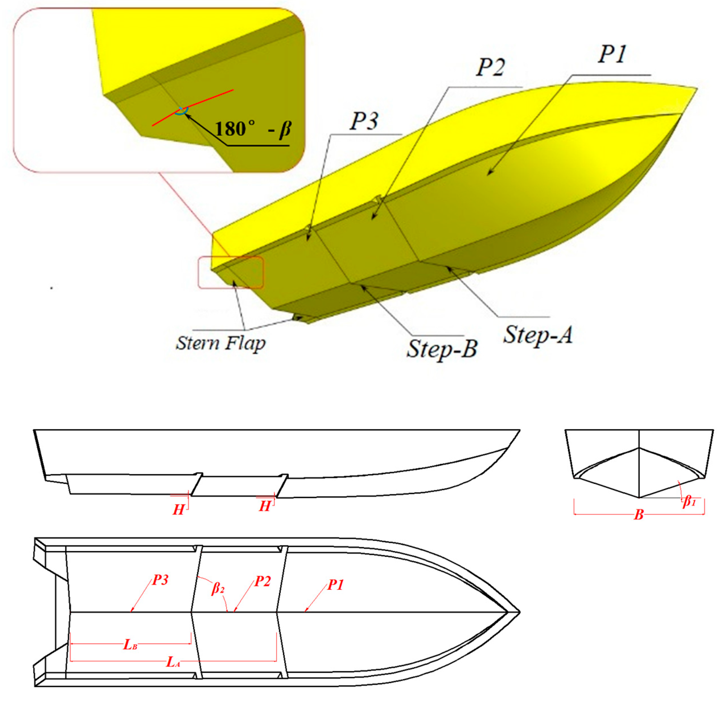
2.1. Geometrical Description of the Hull Model

Teng [19] discussed the height of steps and the longitudinal step position of series DSPBM (double-stepped planing boat model) models. Based on that work, we selected DSPBM as the parent ship, and combined with the performance and research experience, an optimized model was introduced. The geometry of the hull and step configuration are shown in Figure 1. It can be seen that two V-type steps are introduced to the planing hull bottom along the longitudinal direction. Hence, the planing bottom is divided into three segments, which are identified as the first, second and third planing faces, abbreviated as P1, P2 and P3 from the bow to rear. In addition, to study the effects of stern flap mounting angle on the stepped planing hull, two stern flaps with a length of 4.5% L were mounted to both sides of the bottom. The lifting surface was connected to the planing face, and the chine line was adapted to the flap at the bilge, so as to remain consistent with the hull. During the test, the stern flap mounting angle is defined as the spatial acute angle between the surface of P3 and the stern flap. The flap was mounted in a fixed form with angles of 2°, 3° and 4.5°. The principal dimensions of the hull are defined as follows: The overall length L was 2370 mm, and the beam between the chine line B was 646 mm. As for the longitudinal center of gravity, it has a significant impact on both resistance and stability performance. Therefore, the hull gravity center was set at 0.3 L, referring to the set value of the parent hull, which has both appropriate resistance and stability performance [19]. The exact longitudinal center of gravity X g was 700 mm. The rest of the main characteristics are given in Table 1.

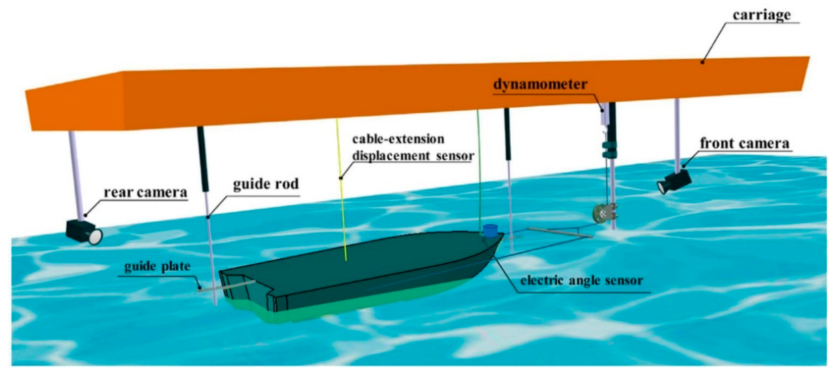
2.2. Experimental Setup

The towing tank test of the double-stepped planing hull model was carried out in the towing tank of the China Special Vehicle Research Institute (also called the NO. 605 Subsidiary Research Institute, Aviation Industry of China Group). The main dimensions were: length 510 m × width 6.5 m × depth 6.8 m. As the corollary carriage towing system can reach a speed range of 0.1 m/s to 22 m/s, with a stable speed error under 0.1%, the maximum length towing tank in China adequately met the requirements of the test. Figure 2 shows a setup schematic overview of the experimental test. The double-stepped planing hull model was fixed to the carriage with the pitch and heave set to two degrees of freedom. In detail, the measuring device and sensors were arranged as follows:
Two guide rods were introduced and mounted in the front and back of the model, preventing yaw and roll motions. The towing point at both broadsides aligned with the gravity center, avoiding a longitudinal movement being produced during the towing process. During the towing tests, a resistance dynamometer was mounted on the carriage to measure the resistance, a cable-extension displacement sensor was mounted at the gravity center, measuring the value of sinkage, and the trim angle was measured by an angle sensor attached to the foredeck. All devices used for data acquisition have regularly been calibrated. After these device and sensor arrangements were set up, to monitor the wave-making characteristics, two cameras were mounted before and after the model.
The towing test was strictly conducted following the ITTC Recommended Procedures and Guidelines [20,21]. During each run, the experimental data such as resistance, sinkage and trim acquisition began after a steady speed had been reached. As for the data post-processing, the experimental data is the mean value derived from an integration of the instantaneous measured values over the same measuring interval, with the zero measurements being subtracted from the average values. In the model tests, three different stern flap mounting angle conditions were considered for β = 2°, 3° and 4.5°. Calm water towing tests were carried out at speeds ranging from 0.44 to 6.13 in Froude numbers. For each angle condition, when the porpoising phenomenon occurred, the towing test process was terminated.

2.3. Experimental Results and Analysis

In this paper, a series of tests were carried out under different conditions of heave, pitch, and total resistance, at different speeds. In addition, according to the camera records, the hull wave-making and motion attitudes were also observed. This information was advantageous to the auxiliary analysis of the results. Test data dimensionless processing was carried out as follows:
Non-dimensional resistance is defined by the resistance to weight ratio (R/Δ). Non-dimensional speed is defined by volume based on the Froude number, following the equation:
F r = V g ( ) 1 / 3
where V is the test speed, and is the displacement of the model. Non-dimensional sinkage is defined by the equation:
δ = δ exp T ¯ ,
where δexp is the experimental trim angle and sinkage value, and T ¯ is the static average draft. In addition, the positive value of trim angle θ and δ represent the increase of the up-pitch and heave.
During the towing test, models with flap mounting angles of 2°, 3° and 4.5° were carried out, respectively. In order to facilitate the discussion in this paper, the series models are named M1, M2 and M3 with the increasing angle of the stern flap. In Figure 3, the non-dimensional resistance, trim, and heave are plotted as functions of the volume Froude number, individually. It can be seen that, after increasing the stern flap angle, the trim and heave of the model were both reduced. Simultaneously, before porpoising, the maximum Froude number that M1 could reach was 5.20, while the maximum velocity of M2 increased to Fr = 5.69; and M3 to 6.13. Thus, for the double-stepped planing boat studied in this paper, increasing the mounting angle stern flap angle can clearly inhibit the porpoising motion.
Table 2 shows the comparison of the dimensionless experimental resistance among different models. The resistance increasing rate is also compared in Table 2, reflecting the effects of flap mounting angle on resistance. A positive value indicates increasing resistance and a negative value indicates reducing resistance. A symbol of “--” indicates when porpoising occurred. At that time, there existed no stable resistance value. It can be observed that when the Froude number was under 3.94, the stern flap played a positive role in improving the resistance performance. Both M2 and M3 achieved a certain resistance reduction effect in this segment of speed. The resistance reduction of M3 was more obvious. At the speed of Fr = 0.88, M3 reached a resistance reducing benefit of 8.9%, while at the resistance hump, the value was 4.9%. With the increase of speed, under the condition of Fr > 3.94, the stern flap had a limited effect on the hull resistance performance. The resistance increased to a slight extent. Compared with the experimental data of M1, the maximum resistance increase was just 1.7%.
According to the experimental data and observations, the stern flap improved the fluid field around the double-stepped planing hull and the longitudinal movement generated by the hydrodynamic lifting force, which not only optimized the double-stepped planing hull motion attitude but also extended the porpoising critical speed. With the flaps’ and steps’ coupled effects, the resistance performance was impacted by the distribution and state of the cavity after the steps, as well as the wetted surface. Specifically, in the medium and low speed segment, the resistance performance was improved, while in the high speed segment, the porpoising inception speed was delayed, with a slight resistance cost.

3. Numerical Simulation Setup

According to the experimental data analysis and observations above, the tested planing hull coupled flaps and double steps show favorable resistance performance at medium and low speed. Furthermore, they also play a positive role in inhibiting porpoising, with a slight resistance cost. However, the mechanism and process of the coupling effect deserve in-depth analysis and research. For this reason, the numerical simulations were carried out based on the model tank towing test. The Froude number ranged from 0.88 to 5.20.

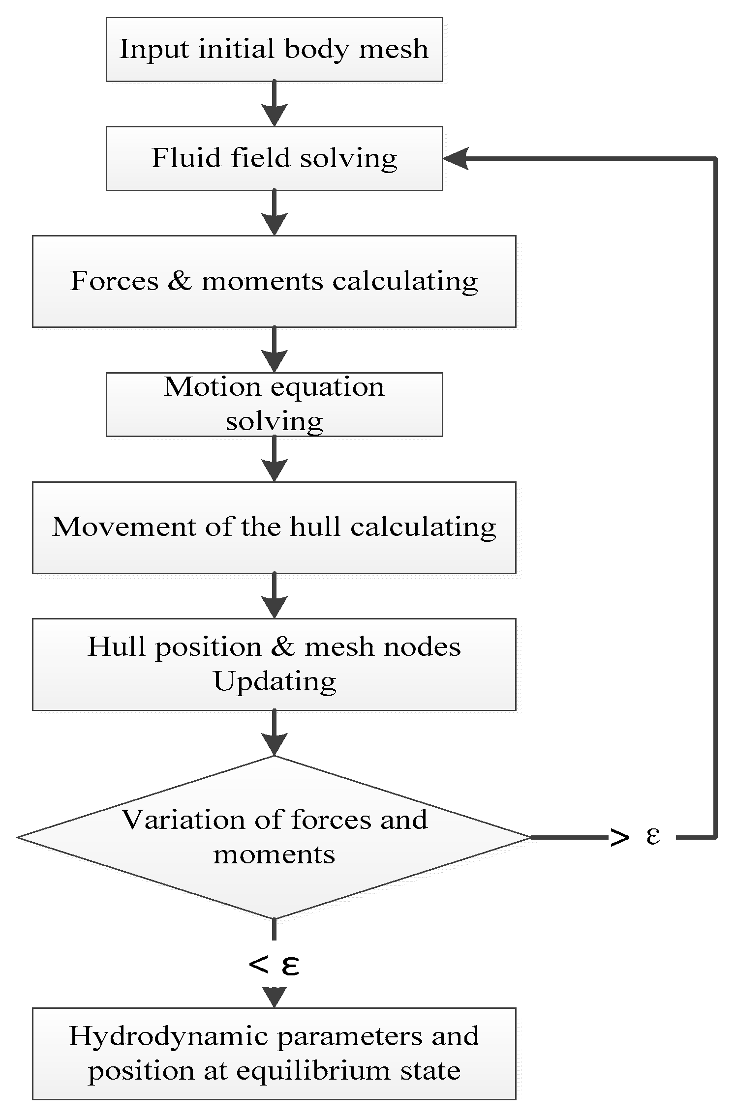
3.1. Mathematical and Numerical Models

As mentioned, the numerical simulations were carried out at the whole speed segment, where the Froude number ranged from 0.88 to 5.20. The speed distribution and stern flap mounting angles were consistent with the trial conditions. In order to establish the solving system of the incompressible viscous flow field surrounding the hull, FVM (finite volume method) software CFX was adapted for use in this paper. As for the simulation of incompressible viscous flow, the RANS (Reynold-Averaged Navier–Stokes) equation method was adopted for solving the Navier–Stokes (N–S) equations. The continuity equations and Reynolds average from the N–S equations are written as:
ρ t + ( ρ u i ) x i = 0 ,
( ρ u i ) t + ( ρ u i u j ) x i = p x i + x j ( μ u i x j ρ u i u j ¯ ) + ρ g i ,
where ui, uj represent the components of the velocity vector, p is the pressure, ρ is the density of the fluid, μ is the coefficient of dynamic viscosity, and ρ u i u j ¯ is the Reynolds stress.
The SST (shear stress transfer) k-ω turbulence model was introduced to close the system, and the wall function was used for the near wall treatment. The coupling of pressure and velocity was realized with the SIMPLE algorithm. Concretely, the transport equations for k and ω are written as:
t ( ρ k ) + x i ( ρ k u i ) = x i ( Γ k k x i ) + G k Y k ,
t ( ρ ω ) + x i ( ρ ω u i ) = x i ( Γ ω ω x i ) + G ω Y ω + D ω ,
where Gk and Gω represent the turbulence kinetic energy generation items, and Yk and Yω represent the turbulence dissipation rate of k and ω, respectively.
As for the free surface, the VOF (volume of fluid) method was introduced to simulate the evolution procedure. At the initial moment, the free-surface height was defined as Hw, while the mesh height was Z. Further, the volume fraction of air–water was defined as:
V a i r = s t e p ( Z H w ) ,
V w a t e r = 1 V a i r ,
If Z-Hw > 0, then Vair = 1. This indicates a total air phase mesh; if Z-Hw < 0, then Vwater = 1. This situation indicates a total water phase mesh. When Z-Hw = 0, Vair = Vwater = 0.5, it represents the distribution here is a free surface. Thus, the air–water phase in the whole flow domain is decided.
In the process of finding the discrete flow field by using the finite volume method, due to the strong directivity of the convection, a high resolution scheme was adopted to discretize the convection term.
In the towing test, the heave and trim angle were measured to describe the motion. Thus, during the numerical simulation process, in order to remain consistent with the towing test setups, 2-DOF (2 degrees of freedom, heave and pitch) motions were released. The following force and moment equilibrium motion equations were introduced to solve the resistance, and motion of the hull:
F = m d 2 X d t 2 ,
M = d d t ( I d θ d t ) ,
where I is the gravity center inertia mass matrix of the hull. F and M are the forces and moments calculated by the equations below:
F = s ( [ τ ] p [ I ] ) n d S G ,
M = s ( r r G ) × ( τ p [ I ] ) · n d S ,
where [ τ ] , p [ I ] , and G , respectively, represent the shear stress, pressure, and gravity. S represents the hull surface, and the vectors r and r G represent the displacements of the mesh nodes and gravity center. The main dynamic solver simulating procedure is shown in Figure 4, and the numerical process is mainly carried out as follows:
First, the N–S equation system and the continuity equation were solved based on the initial meshes inputted. After that, the shear stress field and pressure field around the hull surface were integrated to calculate the forces and moments acting on the hull, as described in Equations (7) and (8). Third, by solving Equations (5) and (6), the parameters of velocity, motion acceleration, and displacement were calculated and obtained. Subsequently, the hull positing and mesh node could then be updated. With updated hull position and mesh nodes, a loop computation was carried out to solve the fluid field. The termination criteria of this algorithm were variations of forces and moments stabilizing to approach 0, which suggests that the hull has achieved an equilibrium state and the numerical process can be terminated.

3.2. Boundary Conditions

To simulate the flow field around the double-stepped planing hull, a CFD (Computational Fluid Dynamics) simulation based on the rigid body motion technique was applied, and the calculating domain was primarily established. Concerning the symmetry of the flow, a symmetrical model and domain were introduced, as shown in Figure 5. The dimensions have a significant impact on the computation accuracy and time consumption. Hence, in this study, the domain was established with a total length of about 6 L, which extends 1 L before the front of the model, and 4 L after the rear. The width of the domain was about 1.5 L. Water depth under the free surface was 1 L, and a length of 0.5 L extends above. The initial attitude of the hull was upright floating, which is consistent with the initial model attitude in the tank trial.
The boundary conditions were specified as follows: The top, bottom, and side planes of the domain were defined as free-slip walls. The plane in front of the bow was considered the fluid velocity inlet, where the velocity was set as the trial speeds. On the opposing side of the domain, the plane was considered the outlet of pressure. As for the hull, a rigid and no-slip wall boundary condition was considered. Due to the symmetry principle, the longitudinal center plane was specified as a symmetry plane. Furthermore, the volume fraction function of water and air at both the inlet and outlet plane was applied to determine the location of the free surface.

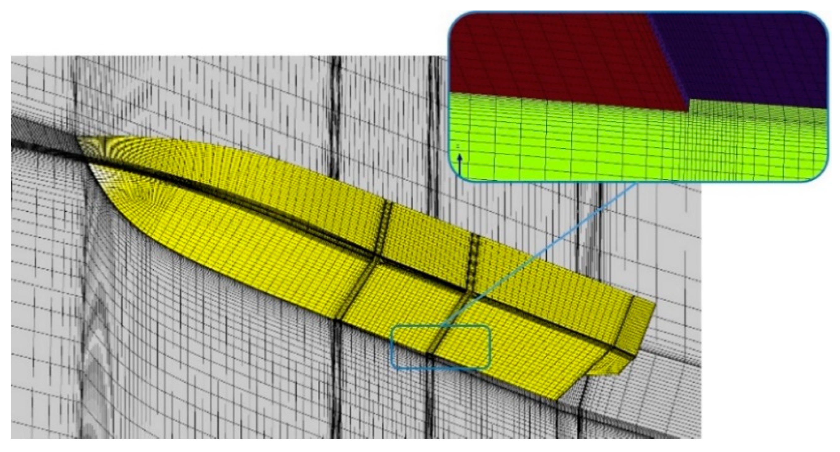
3.3. Mesh Generation and Dependency Analysis

As shown in Figure 6, the whole calculating domain was discretized by a series of structured meshes, and the mesh cells approached the free surface and the hull, as the meshes were refined to accurately capture the flow. Moreover, boundary layer meshes were also carried out around the hull body. As a result, a high resolution inflation layer mesh with dimensionless y+ was near the hull bottom wall around 70, while the y+ was around 50 at the bow. The whole hull near wall dimensionless y+ was around 50~300. In addition, a mesh independence study was conducted to decide an appropriate mesh size.
As for the mesh size, a finer mesh always indicates more precise results, but conversely, it sometimes increases the computational consumption and time cost, due to the large number of mesh elements. Therefore, in order to determine the mesh size with acceptable numerical accuracy and mesh number, a mesh convergence study was carried out, based on a Froude number of 5.20. The mesh at the steps and on hull bottom were gradually refined since the flow around the planing surface has direct influence on the hydrodynamic characteristic of the step. The initial minimum mesh size adopted in the current investigation was 6‰ L. Four mesh plans were made according the refinement ratio of 2 [22]. The total mesh number of each plan and the calculated resistance error (also defined by R / Δ , comparing with the experimental data) were plotted and are shown in Figure 7. As shown in the figure, when the mesh was as fine as Grid3, further refinement would lead to a large increment of element number and hence require more computational time. However, the difference between grid plan 3 and plan 4 was not significant. Therefore, Grid3 was selected as the optimum mesh plan.
The total mesh number was about 9.42 × 10⁵. During the computing course, the physical time step was set at 5 × 10⁻³ s, and the total simulation time step number was 2000.

4. Results and Discussion

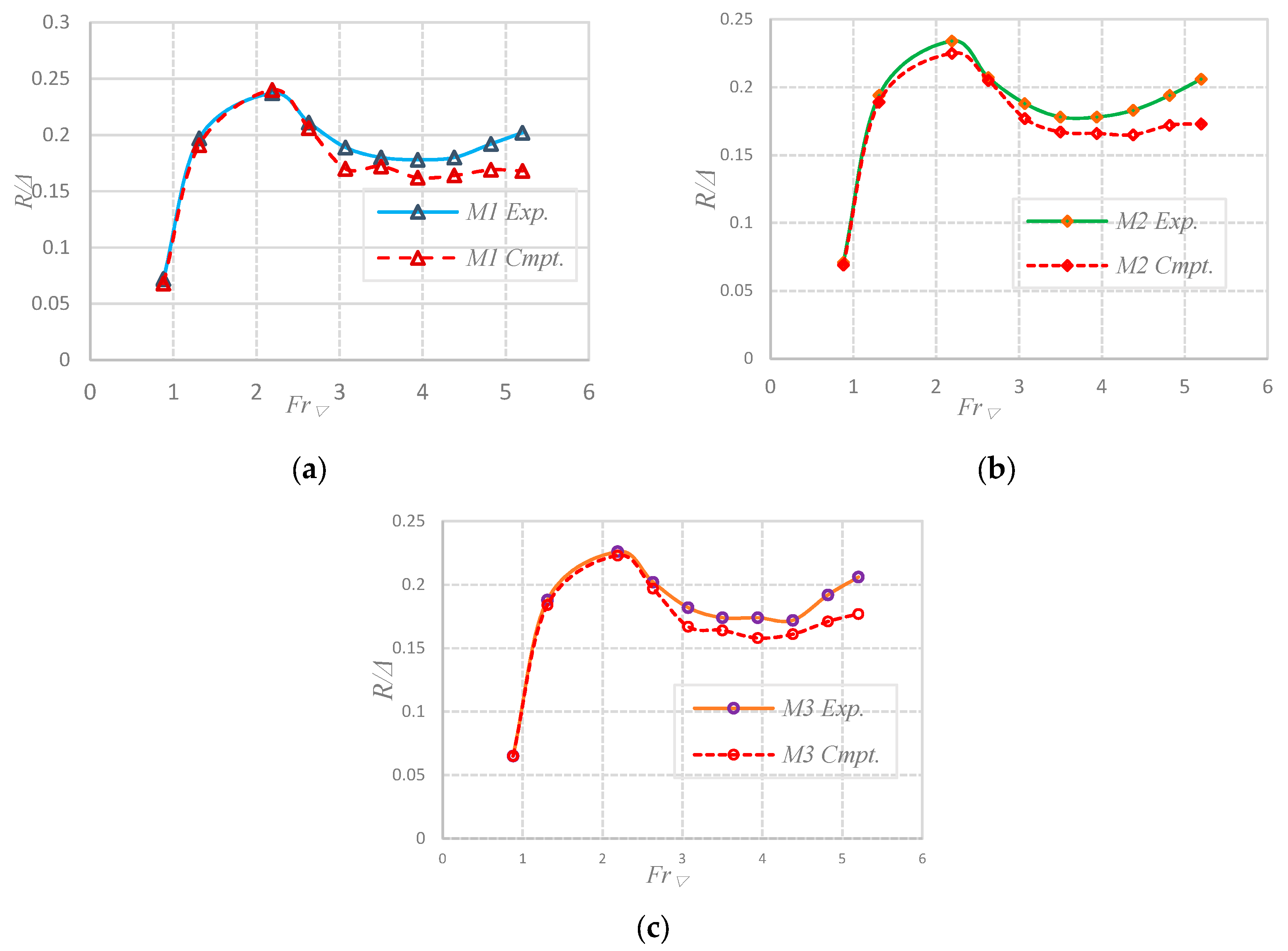
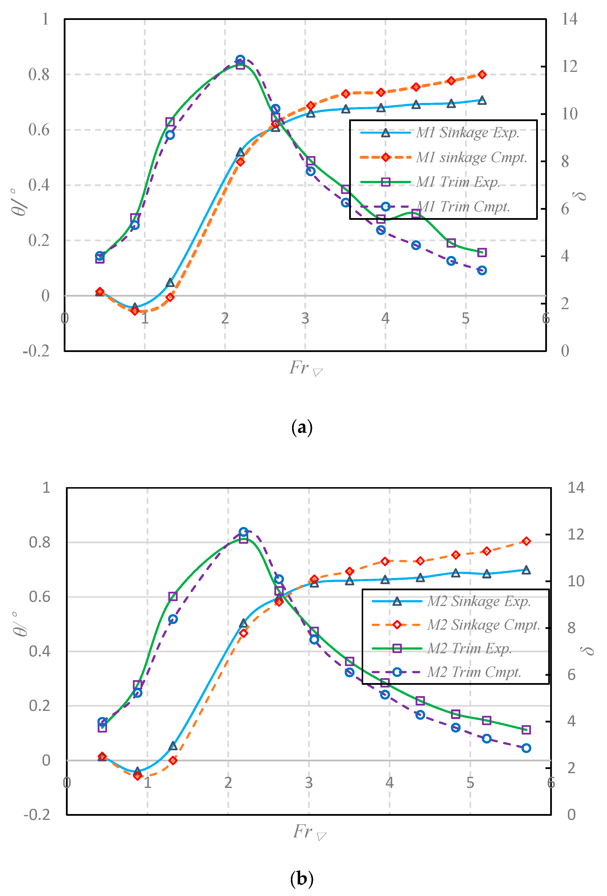
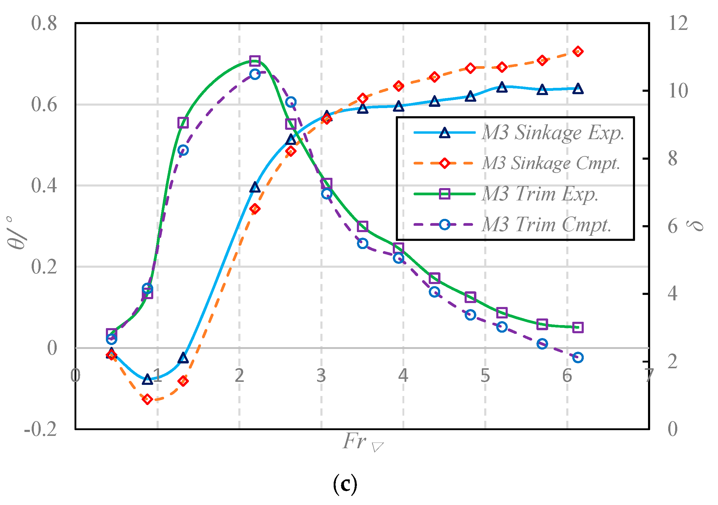
4.1. Validation of the Numerical Method

The evaluation of the numerical simulation was implemented by comparing the wave-making profile between the model test and numerical solution at different velocities. This was also the case for the numerical and experimental resistance values. The numerical method showed an accurate simulation of these characteristics with better anastomosis. Five wave-making profile snapshots of different conditions of model M1 are listed in Figure 8, ranging from a Froude number of 0.88 to 5.20.
At the Froude number of 0.88, the hull trim was small, and the bow generated a water-pushing effect. A wave was generated along the hull, with the wave trough distributed at the midship, while the peak was at the hull stern. With the speed increasing to the Froude number of 2.19, the trim was intensified. An enormous wake flow crest formed at the longitudinal mid-section near the hull stern. At the Froude number of 3.07, the hull stern was lifted by hydrodynamic and aerodynamic lift. The hull reached the planing condition gradually, with trim angle decreasing distinctly. The wake flow crest also departed from the stern and the crest value also showed a slight decrease. The hull had already entered the planing condition at the Froude number of 3.94. The trim angle decrement was slight, and the wave-making kept extending toward the downstream. With the Froude number increased to 5.20, the hull kept planing condition. The trim angle decrement was not obvious, while the hull side wave-making extended to the back slightly.
By comparing the experimental phenomenon with the simulation results, it can be seen that the numerical calculation simulated the flow field accurately. All of the details of the flow field were well demonstrated, and the flow field change of the model test and simulation results were also synchronous.
The computed and numerical errors are summarized in Table 3.
It can be seen from Table 3 and Figure 9 that, under most conditions, the current numerical simulations underestimate the test data. The numerical error of the resistance between the simulation and test data of M1, M2 and M3 varies from 0.36% to 15.89%. However, the resistance curve trend is synchronous for the whole speed segment. In the low speed segment, the computational and experimental result difference is limited. With the increase of speed, the proportion of splash resistance among the total resistance increases gradually. The mesh precision is not enough to simulate the splash phenomenon accurately. Therefore, the error increases gradually. However, by vertically comparing the data of each model, a consistent variation trend of the resistance can be observed. Moreover, both the resistance humps at the speed Froude numbers of 2.19 and 5.20 of the three models are accurately predicted by the numerical simulation. Generally, the numerical simulation results reflect the resistance characteristics of the double-stepped planing hull well, and the resistance difference and variation trend between different models can also be captured precisely.
It can be seen in Figure 10 that, compared with the corresponding simulation results, the testing data of the trim and sinkage are underestimated in most cases. With the increase of speed, the calculated sinkage values increase gradually and they exceed the test data at the speed interval of Froude number 2~3. Both the trim and sinkage discrepancies between the experimental and calculated data increase gradually with the speed. However, a good agreement still can be found between the two groups of curves. The numerical simulation accurately predicts the trend of the two results. Therefore, the validity of the numerical method is approved. The results have a certain credibility and can be used for further flow field analysis.

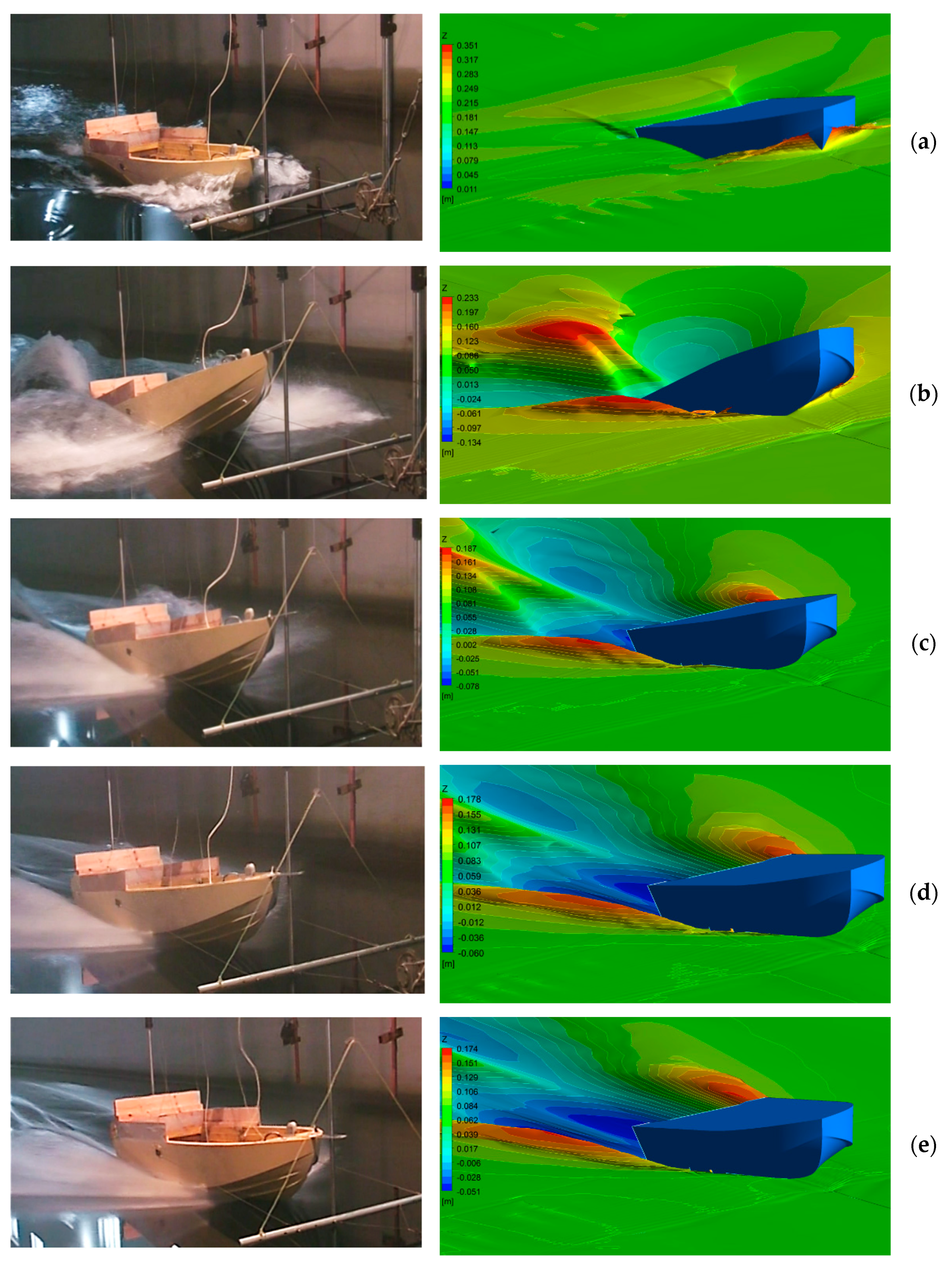
4.2. Cavity and Wetted Surface Analysis

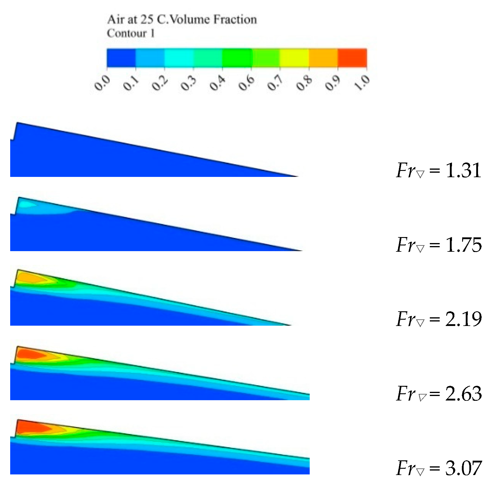
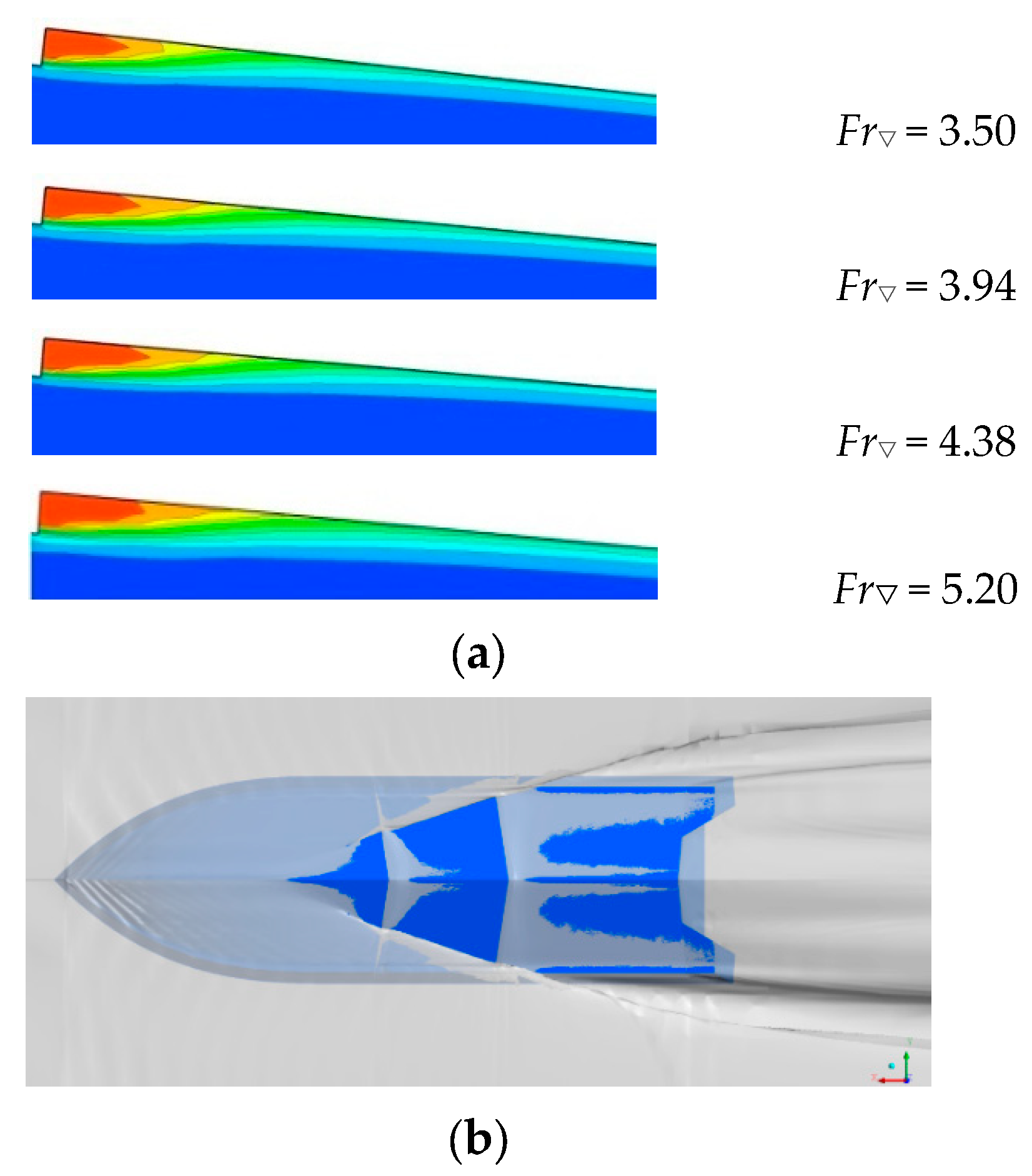
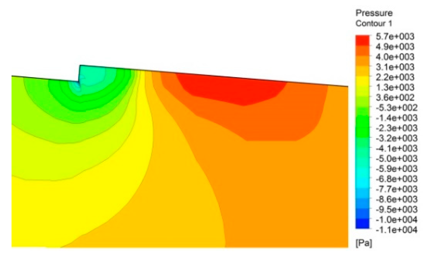
4.2.1. Cavity Behind the Step

During the navigation, with the increase of speed, the cavity after both steps gradually takes shape. To study the formation process and action mechanism of the cavity, the fluid field distribution and morphology evolution under step-B of M1 along the longitudinal center plane at different speeds is extracted. As shown in Figure 11a, the color scale values air volume fractions 0 and 1 represent the complete water phase and gas phase, respectively. It can be observed that at the Froude number of 1.31, only the water phase exists after the step. A small amount of water–air mixture appears at Fr = 1.75, and with the increase of the speed, the component of the gas phase increases gradually. At the Froude number of 2.63, a cavity with a core region entirely in the gas phase is formed. The cavity extends along the longitudinal direction, presenting a sharp wedge-shape with a gas-phase composition that decreases gradually. With Fr continuing to increase, the cavity keeps expanding to the rear at the speed of Froude number 5.20, shown in Figure 11b. The longitudinal length of the cavity gas-phase core region reaches its maximum at about 2.5 times H.
We now discuss the cavity formation and evolution process according to the above analysis. To discuss the formation mechanism, a typical flow field around step-B of M1 was further analyzed at a Froude number of 4.38. Figure 12 shows the pressure distribution of the bottom at the longitudinal center section. The inflow flows through the step, and a low-pressure area is primarily formed behind it, while a distinct high-pressure area is formed at the region where the flow scuds the step and contacts the planing surface again. Due to the effect of two adjacent pressure difference areas, a backflow is developed, as shown in Figure 13. Simultaneously, the flow at both sides of the hull is pushed to the hull bottom along the step. With increasing speed to a certain extent, the terminal of the step is exposed to the air with the hull lifting. As a result, a suction effect is generated by the pressure difference, and the air is pumped into the hull bottom in a cyclone formation. The cavity, as stated, is in essence generated by the low-pressure induced cyclone.

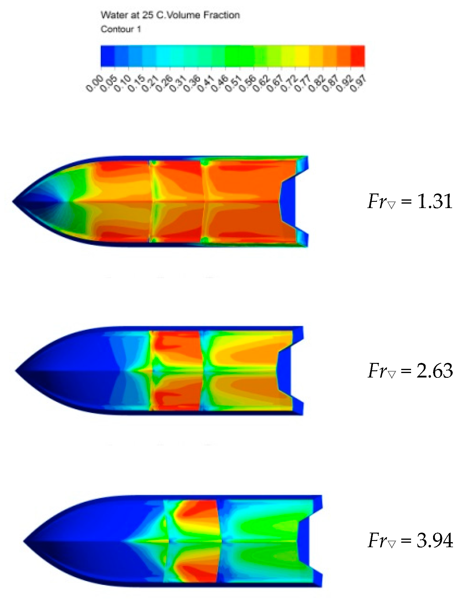
4.2.2. Influence of Steps on the Wetted Surface

To determine the influence of a double step on the wetted surface of the planing bottom, the distribution of the wetted area of the hull M1 under different speeds was extracted. The forms of water volume fraction were used to represent the air–water mixture situation. In order to provide a direct observation of the wetted surface evolution, a bottom view of the hull is displayed in Figure 14. The color scale values 0 and 1 represent the complete gas phase and water phase state, respectively. A value between 0–1 represents corresponding weight gas–water mixtures of the volume fraction. It can be observed that the wetted surface changes are mainly caused by two factors: one is the change of the air–water mixture component caused by the cavity, and the other factor is the shape change of the wetted surface caused by the navigation state.
For the first factor, with the increase of speed, the component of the gas phase increases continuously. Especially at the planing surface of P3, the gas phase increases and forms a relatively complete air cavity. The cavity near the step terminal bulges to the rear, while the middle is sunken to the bow. Correspondingly, the wetted surface is concentrated at the stern and draws close to the middle plane. The wetted surface distribution on planing surface P2 is similar, but clear wetted surface is observed. For the second factor, with the hull lifting and trim variation caused by increasing speed, the stagnation line (the intersecting line of the bow and water surface) collapses gradually. This factor mainly affects the wetted surface variation on planing surface P2.
For further study of the performance of the wetted surface reduction, the wetted surface calculation equation was introduced. The bottom wetted area was computed by integrating the water volume fraction over bottom S. The equation is written as:
A w e t = s V w a t e r d s ,
where Awet represents the wetted area and Vwater represents the water volume fraction at each differential element. The ratio of the calculated wetted area and bottom area Awet/A was introduced to represent the wetted surface reducing effect. The result is plotted as a function of the Froude number and is shown in Figure 15. The wetted surface reduces rapidly with the increase of speed. After the Froude number exceeds 4.38, the ratio remains at a fairly stable value of 0.23. The ratio suggests an obvious effect of the step, which also indicates the action mechanism of the double-step in this study.

4.3. Hydrodynamic Characteristics of the Stern Flap

During navigation, the stern flap is, in essence, a planing plane. Hydrodynamic lift is generated under the flap. Meanwhile, due to the mounting angle, when the fluid flows through the flap a retardative effect occurs in the flow field. As a result, the pressure and movement distribution adjust and vary. The flow field of stern flap M3 at the Froude number of 5.20 is taken as an example for further analysis. As shown in Figure 16, the incoming flow velocity vector line direction shows deflection at the connection of the hull bottom and stern flap. The pressure distribution of the flow field is automatically changed by this effect, shaping a distinct high-pressure region. In addition, a bottom view of the flap is shown in Figure 17. A high-pressure region forms in the shape of a belt. This region has a relatively uniform distribution in the transverse direction. The region covers most of the anterior part of the stern flap in the longitudinal direction.
As mentioned previously, the stern flaps have an obvious influence on the pressure and movement distribution. Clarifying the characteristics of stern flaps is important in the analysis of the flap action mechanism, in order to evaluate the hydrodynamic characteristics of the stern flap. A series of non-dimensional evaluation coefficients were applied during our data process. The non-dimensional pressure coefficient Cp and torque coefficient CMΔ are specified in Equations (14) and (15):
C p = P P r e f 1 2 ρ V r e f 2 ,
C M Δ = M B Δ ,
where P is the local absolute pressure, Pref is the reference pressure, or atmospheric pressure, Vref represents the velocity of the inlet flow, ρ represents the water density and M is the movement generated by the stern flap, referring to the transom axis of the gravity center.
Figure 18 shows the influence of the stern flap mounting angle on pressure distribution along the centerline of the stern plate at a Froude number of 5.20. The non-dimensional pressure coefficient Cp is plotted with a lateral axis of the ratio between longitudinal coordinates of the pressure monitor point and hull length, L. The first monitor point is located at the trailing edge of step-B, while the last monitor point is located at the trailing edge of the flap. The positive coordinates point to the direction of the bow. It can be seen that there are two pressure peaks along the longitudinal direction. The frontal peak is near step-B. As discussed in Section 4.2, this is mainly caused by the flow scudding over the step and making contact with the planing surface again. The latter peak represents the local high-pressure caused by the retardation effect of the flap. Comparing the peak values among M1, M2 and M3, the peak shows a positive correlation relationship with the increasing mounting angle. The peak value and longitudinal range of the high-pressure region gradually increase with an increasing mounting angle, suggesting that the lift is also magnified.
During navigation, the motion attitude of the hull is mainly adjusted by the hydrodynamic lifting force and trimming moment. The torque coefficients of flaps with different mounting angles are plotted in Figure 19, as a function of the Froude number. The minimum trim moment is located at the speed point of Fr = 1.31. After that, with the increase of speed, the trim moment increases gradually. Moreover, the mounting angle increase makes the trim moment generated by the flap increase. Synchronously, not only the trim moment but also its increasing amplitude increase obviously with the speed, rising under the high speed segment. Correspondingly, the motion attitude adjustment ability is improved by enlarging the mounting angle.

4.4. Influence of the Mounting Angle on the Stepped Planing Hull

As discussed in Section 4.2, salutatory changes were introduced to the stepped hull bottom. When the inflow flows through the steps, cavities are formed on account of the pressure difference. The cavities cover the hull bottom, which decreases the wetted surface area, and reduces the friction resistance. Therefore, the size of the cavity is an important factor that affects the resistance performance of stepped planing hulls. In this section, the models of M1, M2 and M3 with different mounting angles are examined and compared to evaluate the evolution process and mechanism of cavitation under different angle configurations.
As shown in Figure 20, a comparison of the cavity morphology after step-B has been carried out. The cavity morphologies are grouped by different velocity cases in which the Froude number is 2.63, 3.50, 4.38 and 5.20. It can still be observed that the core region of the cavity is dominated by the gas phase, while the periphery of the core region is a mixture of water and gas. As the speed increases, the cavity expands toward the rear. As for different models at the same speed, when in the crossing mode (Fr = 2.63), the cavities are in the initial shaping stage where the cavity shape and size are not significantly different from each other. With the increase of the speed, after the hull enters the planing state (Fr ≥ 3.50), the cavitation expanding rate varies in each model. The expanding rate of M3 is the most rapid, and M2 is second, while M1 is the minimum. Therefore, after the hull enters the planing state, the cavity expands with the increasing flap mounting angle. Similarly, the expanding of the cavity reduces the wetted surface and friction resistance, which indicates that the resistance increase caused by the flap mounting angle increasing is small in scale.
To study the influence of stern flap mounting angle on the hydrodynamic performance of the hull curves, the load coefficient is plotted as a function of the Froude number. The curves are divided into three groups based on the difference of the planing surface. The load coefficient is defined as:
C Δ n = Δ n Δ ,
where Δn is the load on each planing surface. The subscript n is valued as 1, 2, and 3, representing different planing surfaces. CΔ1,2,3 correspond to P1, P2 and P3, as defined in Figure 1. As is shown in Figure 21, the load coefficient curve of different models has basically the same trend in every specific planing surface. The load of the planing surfaces is mainly affected by the flap mounting angle in the following two modes.
The first mode directly affects the load on the planing surface by changing the motion attitude. This mode mainly acts on P1 and is reflected in the curves of CΔ1. Due to the increase of the stern flap mounting angle, the trim and heave during navigation are both reduced. This will inevitably lead to the increase of the wetted surface at P1, and correspondingly, the load coefficient CΔ1 also increases with the increasing mounting angle.
The other mode affects the planing surface load indirectly by changing the shape of the cavity. This mode acts on P2 and P3 and is reflected in the curves of CΔ2 and CΔ3. Combined with the cavity morphology comparison in Figure 20, due to the increase of the mounting angle, the cavity expands to the hull rear, resulting in a decrease of the wetted surface and the load coefficient. Thus, with the increase of the mounting angle, an opposite trend is obtained in CΔ2 and CΔ3 from the load coefficient variation trend of CΔ1.
Furthermore, among the curves from CΔ1 to CΔ2, the uniformity of the load distribution before and after the gravity center is improved with the increasing flap angle. As discussed above, after the hull enters the planing state, the cavity expands with the increasing flap mounting angle. The main cause should be that the flaps reduce the trim angle by improving the planing surface load distribution, which in turn leads to the cavity length increasing. As a result, once the hull is disturbed from its equilibrium position, the planing surfaces can provide a fairly effective restoring movement. Under the action of the restoring movement, the hull can rapidly return back to the equilibrium position, which suggests that increasing the stern flap mounting angle can achieve the delaying of porpoising.

5. Conclusions

In this paper, an experimental and numerical combined study for the double-stepped planing hull has been carried out, and the focus has been mainly on the hydrodynamic characteristics of the step and stern flap, as well as the coupling effect on the hull body. The cavity formation and evaluation process after the step have been captured with acceptable accuracy. Furthermore, the effects of coupled steps and stern flap mounting angles have been investigated, and their action mechanism and effects on resistance performance and porpoising inhibition have been discussed and summarized. Based on the presented results and analysis, the main conclusions can be drawn as follows:
(1)
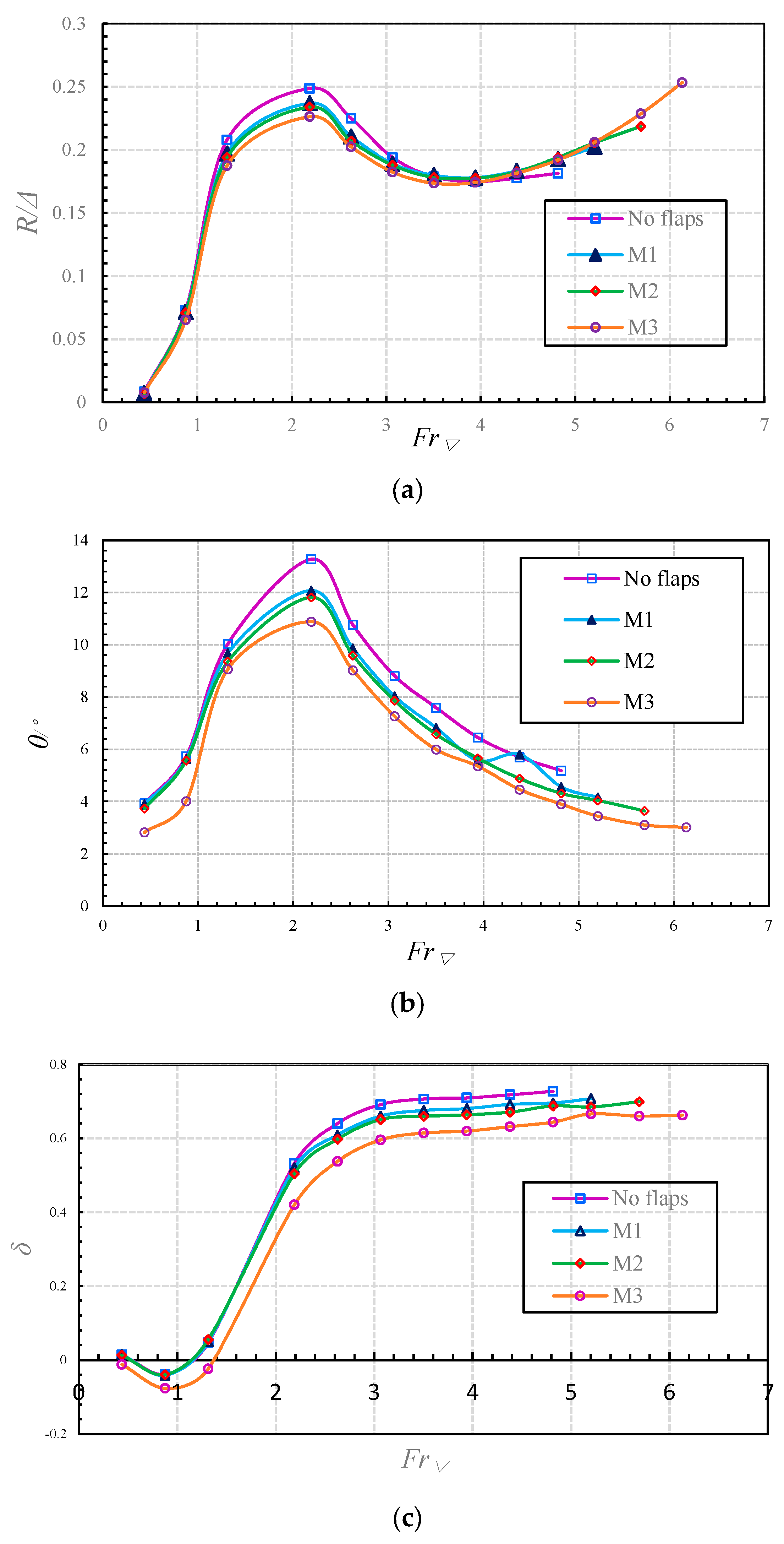
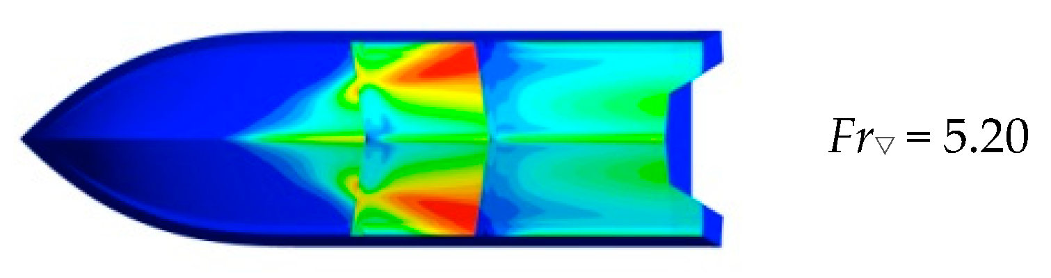
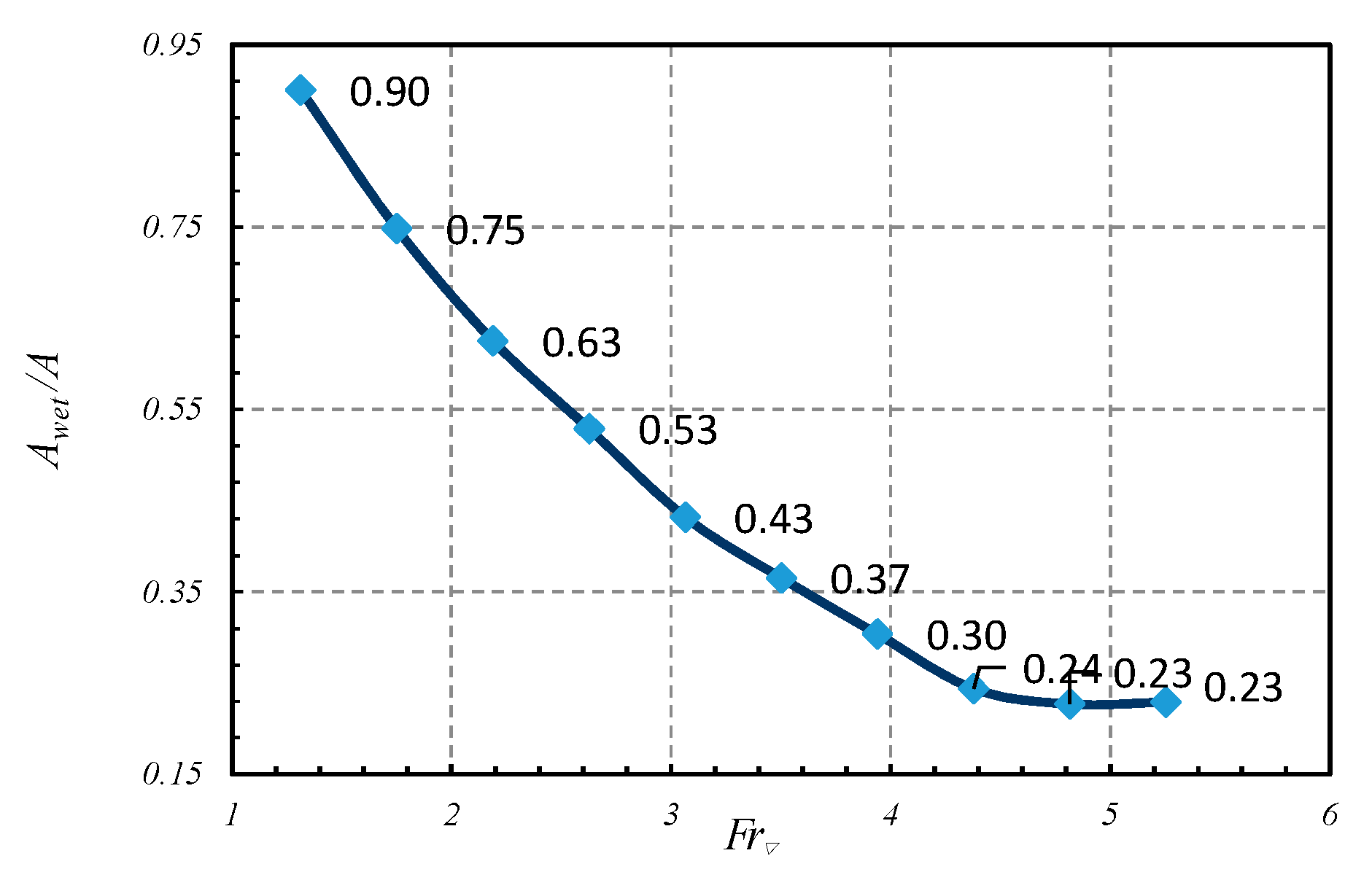
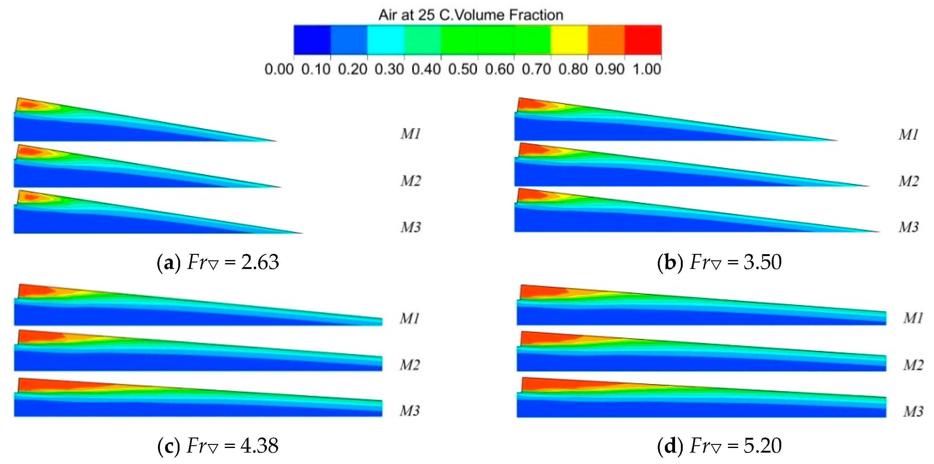
The low-pressure region caused by the step saltation is the immediate induction of the cavity. With a speed increase, the cavity expands toward the rear, increasing the cavity coverage area. Conversely, the wetted surface area decreases. As for the distribution, the wetted surface is mainly concentrated in the post-median part of a planing surface. After the Froude number exceeds 4.38, the ratio of the wetted area and bottom area Awet/A remains at a fairly stable value of 0.23. The decrease of the wetted surface indicates the steps’ friction resistance reducing mechanism.
(2)
The stern flap is an effective resistance and motion regulating device. Enlarging the stern flap mounting angle within the variation range improves the resistance performance obviously. Moreover, it has a significant porpoising inhibition effect, with a slight cost of resistance during the high speed segment. The maximal porpoising critical speed extends with the increase in the mounting angle.
(3)
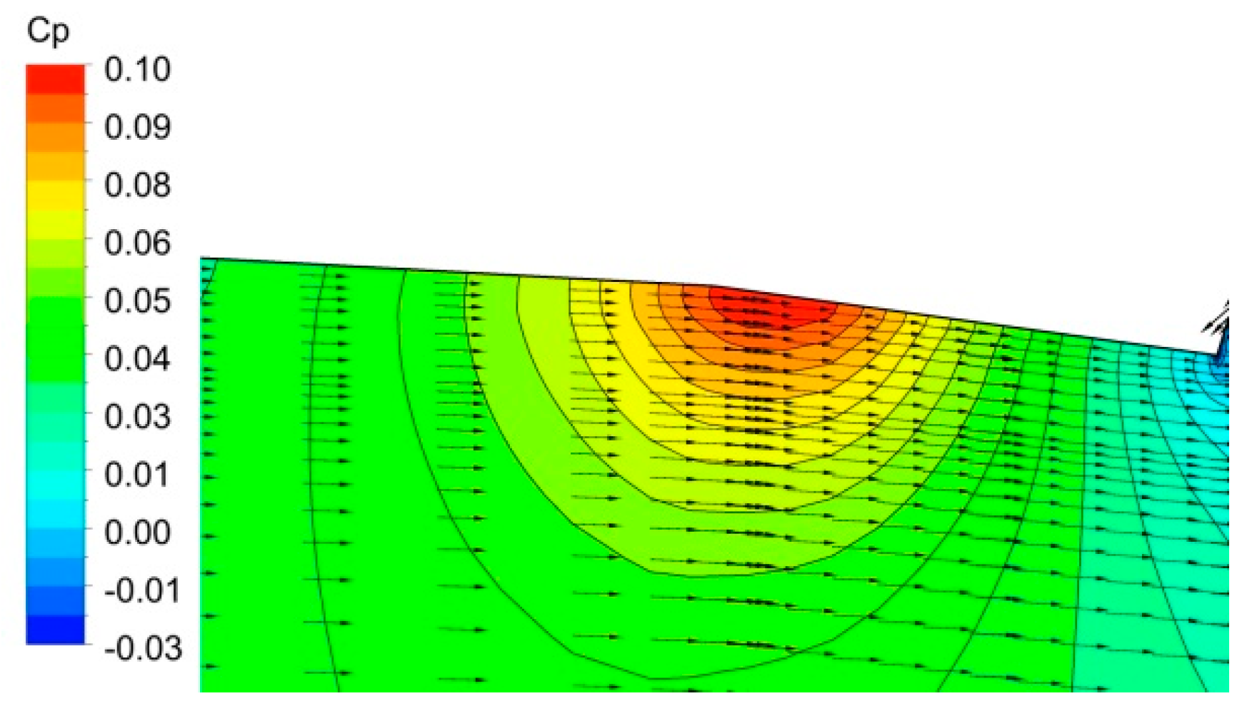
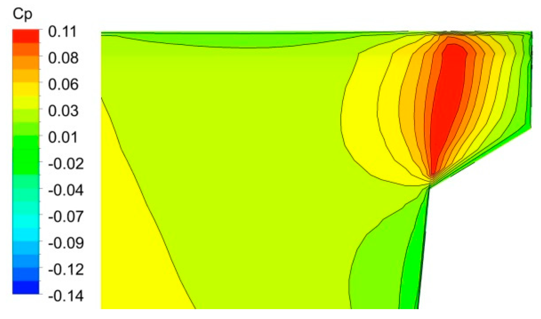
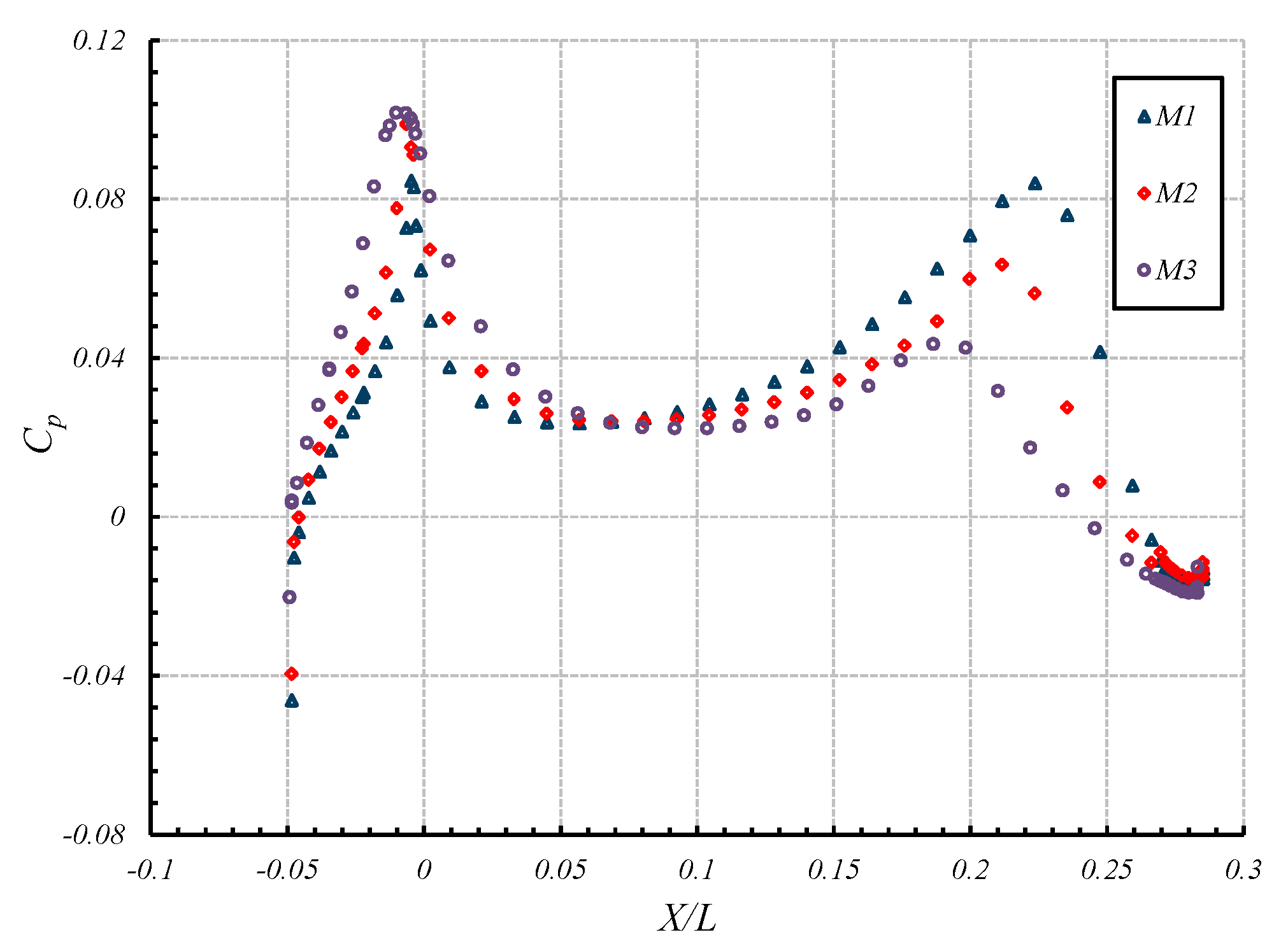
The connection position of the stern flap and hull is a high-pressure concentration area. With the increase of the mounting angle, the pressure value and the trim moment of the stern flap also increase. Correspondingly, the hull motion regulating ability is also improved.
(4)
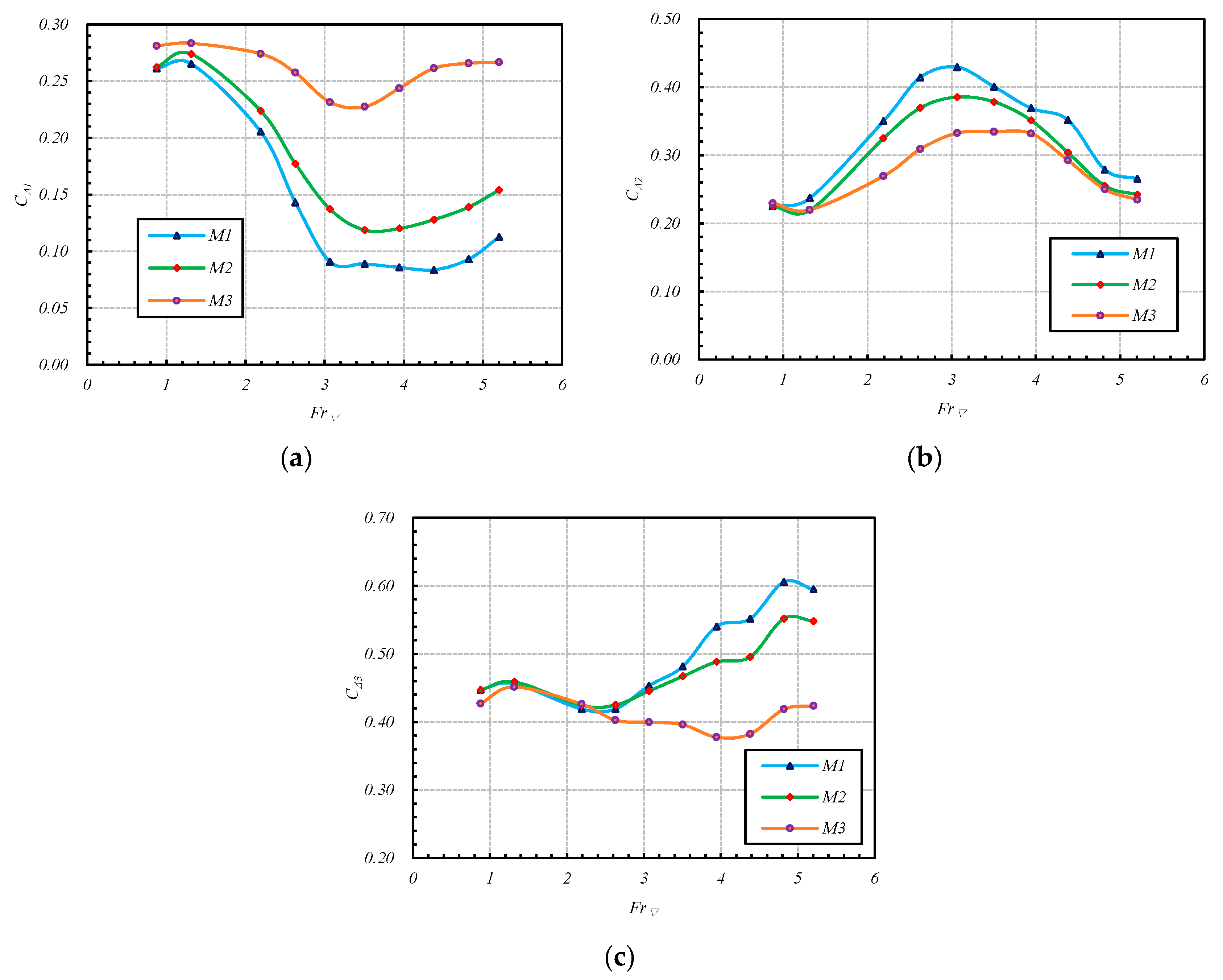
Increasing the stern flap mounting angle reduces the trim, and intensifies the cavity expansion speed. The wetted surface area shrinks; the friction resistance is reduced. Therefore, the total resistance amplification is slight. In the meantime, the load among the planing surfaces distributes more uniformly with the increasing flap angle, which is also beneficial for inhibiting porpoising.

Author Contributions

Conceptualization, J.Z.; Formal analysis, Y.J. and S.L.; Investigation, S.L., Z.L. and Y.J.; Methodology, S.L., J.Z. and H.S.; Resources, Y.J. and Z.L.; Supervision, J.Z.; Validation, H.S.; Writing—Original draft, S.L.; Writing—Review and editing, S.L. and J.Z.

Funding

The research was funded by Opening Foundation of State Key Laboratory of Ocean Engineering of China (1617), Key Laboratory Fund (614222303030917) and National Science of Foundations of China grant numbers 51509055.

Conflicts of Interest

The authors declare no conflict of interest. The funders had no role in the design of the study; in the collection, analyses, or interpretation of data; in the writing of the manuscript, or in the decision to publish the results.

Appendix A

In the mesh independent study, the total resistance is the main studied and analyzed element. Furthermore, the domain dependence study is also conducted to confirm a sufficiently large and acceptable computational domain.
The initial computational domain size is chosen referring to a similar stepped-planing hull simulation study [12]. The domain is established with a total length of about 6 L, which extends 1 L before the front of the model, and 4 L after the rear. The width of the domain is about 1.5 L. Water depth under the free surface is 1 L, and a length of 0.5 L extends above.

Appendix A.1. Width and Length Study of the Domain

Due to the symmetry principle, the practical simulating width is about 3 L, while in the experiment, the width of the towing tank is 6.5 m (2.74 L). It indicates that the domain width is wide enough to simulate the experimental facility. The side wall is defined as free slip walls. With the initial domain setup, several speed conditions of M1 are simulated. The results of the wave making after the hull of model M1 at different speeds are shown in Figure A1. It can be seen that the wave making is slightly more toward the side wall. With the speed increase, the wave-making area is narrowed down from the side wall and is extended along the longitudinal direction. However, the wave making area is still distributed in the calculation domain. Therefore, the waves reflect off the side boundaries and have very limited influence. Additionally, the domain outlet, the size of the domain that is downstream from the hull, is enlarged to 4 L, making the results insignificant for this size. Therefore, the width and length of the domain is accepted.
Figure A1. Wave making after the hull of model M1 at different speeds.
Jmse 07 00346 g0a1

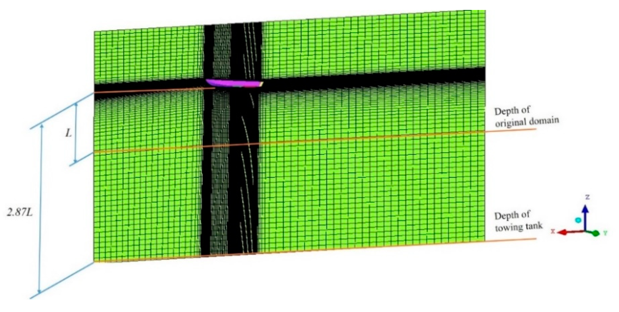
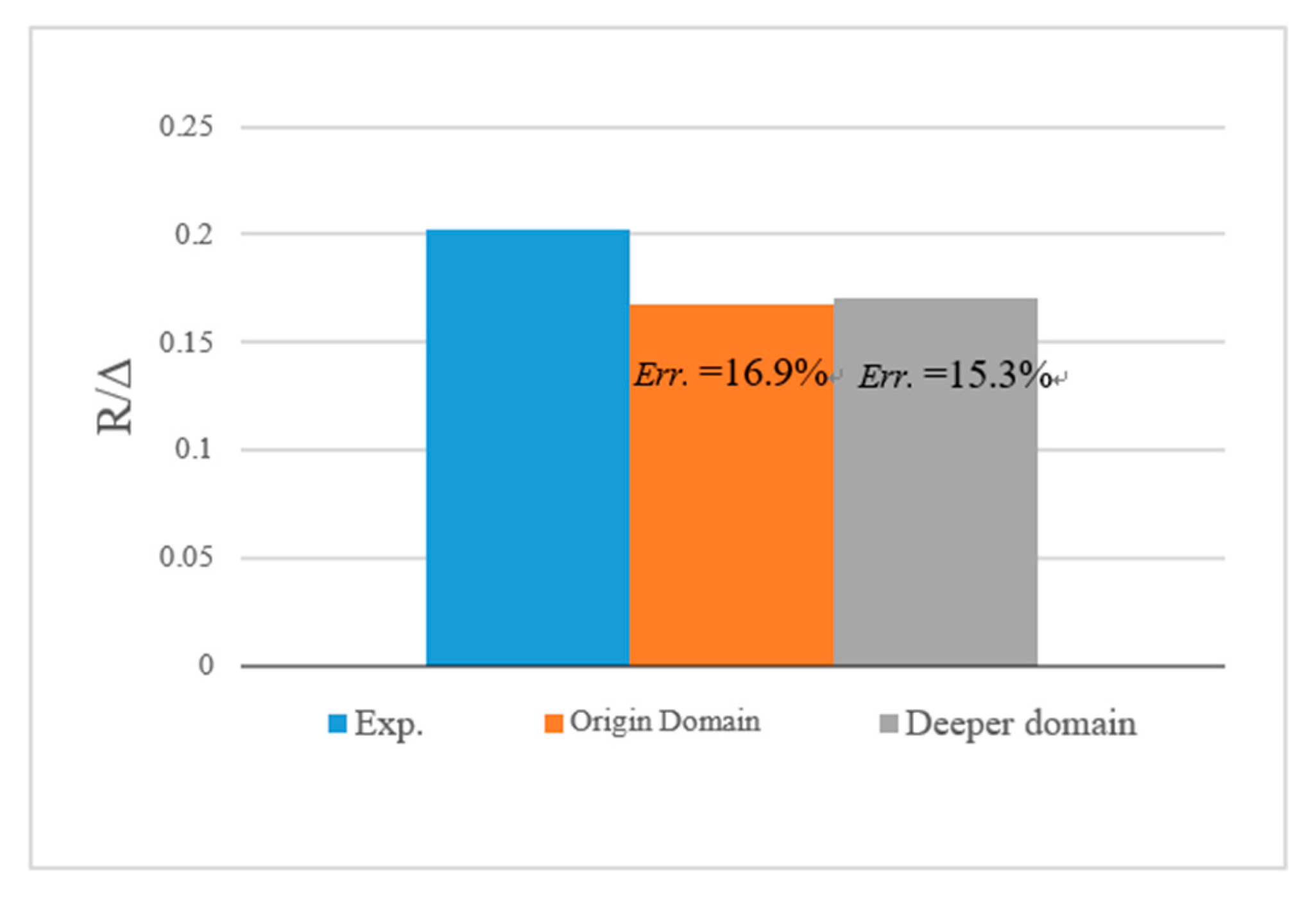
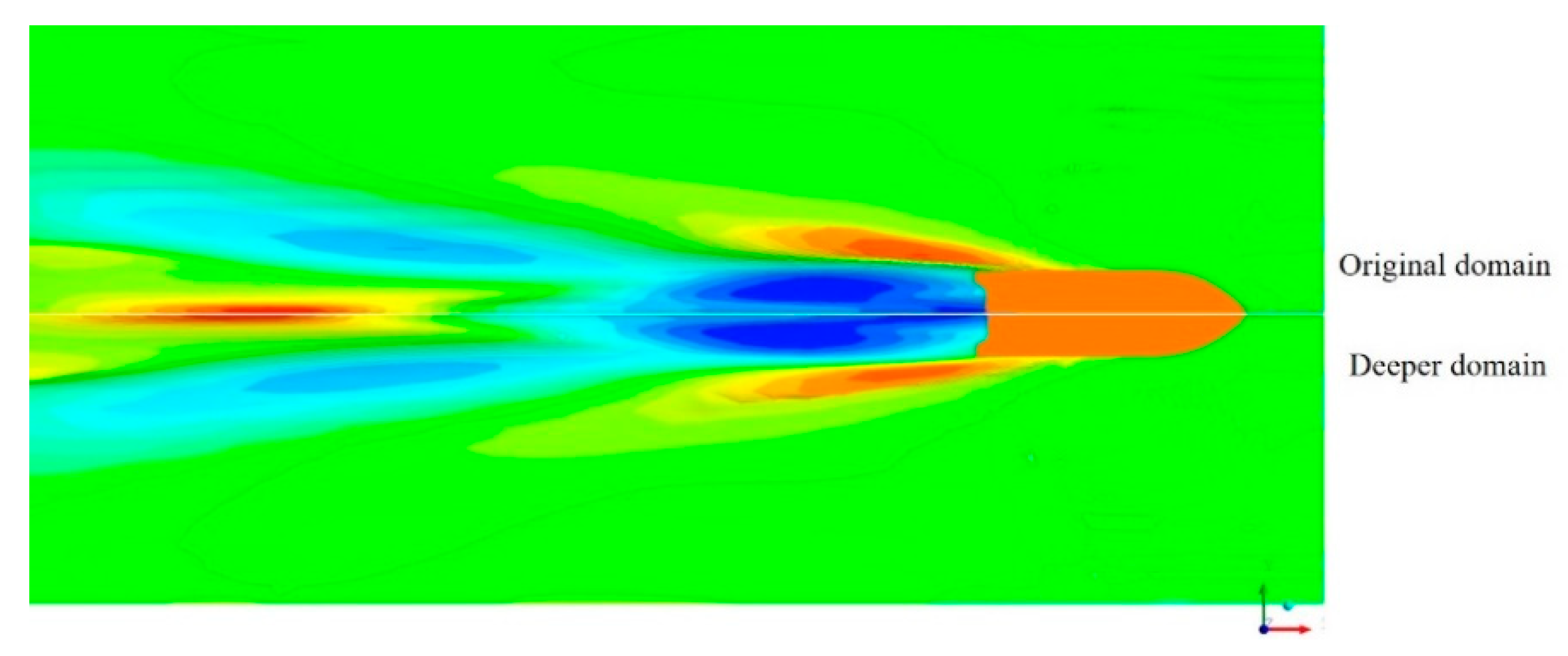
Appendix A.2. Depth Study of the Domain

The initial depth of the calculation domain is 1 L, while the towing tank depth is 6.8 m (2.87 L). To verify domain depth independence, a simulation for the hull model with the initial depth, and another calculation domain, where the domain depth matches the experimental facility, is carried out. The remaining parts of the domain setup stay the same. Figure A2 below shows the comparison of domain depth.
Figure A2. Depth comparison between original and deeper domain.
Jmse 07 00346 g0a2
The calculated results between original and deeper domains are shown in Figure A3 and Figure A4. It can be seen that using the deeper domain could slightly improve the numerical accuracy in drag prediction and weaken the influence of hull body on the domain bottom, which makes the simulation closer to the experimental data. However, by comparing the wave pattern of the free surface and numerical resistance data, the enlargement of the deeper domain does not show obvious improvement with the mesh increasing sharply. Therefore, the results of the initial domain depth still satisfy the research requirements.
Figure A3. Calculated resistance and numerical accuracy.
Jmse 07 00346 g0a3
Figure A4. Calculated wave-making of the original domain (upper half) and deeper domain (lower half) M1 at Fr = 5.20.
Jmse 07 00346 g0a4

Appendix A.3. Conclusions

As discussed above, the domain dependence study shows good results for the original domain. The width and length of the initial domain meet the accuracy demands for the simulation. Although the calculating domain is physically shallower than the towing tank and the deepened domain can slightly improve the numerical accuracy, the original domain can also capture the flow field details and trends well, and with less cost. Therefore, the initial domain is selected as the calculation domain.

References

  1. Zheng, Y.; Dong, W.C.; Yao, C.B. Experimental study on resistance reduction of displacement type Deep-V hull model using stern flap. J. Shanghai Jiaotong Univ. 2011, 45, 475–479. [Google Scholar]
  2. Maki, A.; Arai, J.; Tsutsumoto, T.; Suzuki, K.; Miyauchi, Y. Fundamental research on resistance reduction of surface combatants due to stern flaps. J. Mar. Sci. Technol. 2016, 21, 344–358. [Google Scholar] [CrossRef]
  3. Savitsky, D. Hydrodynamic design of planing hulls. Mar. Technol. 1964, 1, 71–95. [Google Scholar]
  4. Villa, D.; Brizzolara, S. A systematic CFD analysis of flaps/interceptors hydrodynamic performance. In Proceedings of the 10th International Conference on Fast Sea Transportation FAST, Athens, Greece, 5–8 October 2009; pp. 1032–1038. [Google Scholar]
  5. Karimi, M.H.; Mohammad, S.S.; Majid, A. A study on vertical motions of high-speed planing boats with automatically controlled stern interceptors in calm water and head waves. Sh. Offshore Struct. 2015, 10, 335–348. [Google Scholar] [CrossRef]
  6. Celano, T. The prediction of porpoising inception for modern planing craft. Trans. Soc. Nav. Archit. Mar. Eng. 1998, 106, 269–292. [Google Scholar]
  7. Lee, E.; Pavkov, M.; McCue, W.L. The systematic variation of step configuration and displacement for a double-step planing craft. J. Sh. Prod. Des. 2014, 30, 89–97. [Google Scholar] [CrossRef]
  8. Garland, W.; Maki, K.J. A numerical study of a two-dimensional stepped planing surface. J. Sh. Prod. Des. 2012, 28, 60–72. [Google Scholar] [CrossRef]
  9. Morabito, M.G.; Pavkov, M.E. Experiments with stepped planing hulls for special operations craft. Trans. Roy. Inst. Nav. Archit Part B Int. J. Small Cr. Technol. 2014, 156, 87–97. [Google Scholar] [CrossRef]
  10. DeMarco, A.; Mancini, S.; Miranda, S.; Scognamiglio, R.; Vitiello, L. Experimental and numerical hydrodynamic analysis of a stepped planing hull. J. Appl. Ocean Res. 2017, 64, 135–154. [Google Scholar] [CrossRef]
  11. Garland, W.R. Stepped planing hull investigation. Trans. Soc. Nav. Archit. Mar. Eng. 2012, 119, 448–458. [Google Scholar]
  12. Lotf, P.; Ashrafzaadeh, M.; Kowsari, E.R. Numerical investigation of a stepped planing hull in calm water. Ocean Eng. 2015, 94, 103–110. [Google Scholar] [CrossRef]
  13. Makasyeyev, M.V. Numerical modeling of cavity flow on bottom of a stepped planing hull. In Proceedings of the 7th International Symposium on Cavitation, Ann Arbor, MI, USA, 17–22 August 2009. CAV2009-116. [Google Scholar]
  14. Morabito, M.G. Empirical equations for planing hull bottom pressure. J. Sh. Res. 2014, 58, 185–200. [Google Scholar] [CrossRef]
  15. Ghadimi, P.; Tavakoli, S.; Dashtimanesh, A.; Zamanian, R. Steady performance prediction of a heeled planing boat in calm water using asymmetric 2D+t model. Proc. Inst. Mech. Eng. Part M J. Eng. Marit. Environ. 2016, 231, 234–257. [Google Scholar] [CrossRef]
  16. Dashtimanesh, A.; Esfandiari, A.; Mancini, S. Performance Prediction of Two-Stepped Planing Hulls Using Morphing Mesh Approach. J. Ship. Prod. Des. 2018, 34, 236–248. [Google Scholar] [CrossRef]
  17. Veysi, S.J.; Bakhtiari, M.; Ghassemi, H.; Ghiasi, M. Toward numerical modeling of the stepped and non-stepped planing hull. J. Braz. Soc. Mech. Sci. Eng. 2015, 37, 1635–1645. [Google Scholar] [CrossRef]
  18. Ghadimi, P.; Panahi, S.; Tavakoli, S.J. Hydrodynamic study of a double-stepped planing craft through numerical simulations. Braz. Soc. Mech. Sci. Eng. 2019, 41, 2. [Google Scholar] [CrossRef]
  19. Xin, T. Analysis on Hydrodynamic Performance of Double-stepped Planing Craft and its Appendages. Master’s Thesis, Harbin Engineering University, Harbin, China, 2014. [Google Scholar]
  20. ITTC. Recommended Procedures and Guidelines: General Guidelines for Uncertainty Analysis in Resistance, 7.5-02-02-02. In Proceedings of the International Towing Tank Conference, Copenhagen, Denmark, 1–5 September 2014. [Google Scholar]
  21. ITTC. Recommended Procedures and Guidelines: Testing and Extrapolation Methods Resistance Resistance Test, 7.5-02-02-01. In Proceedings of the International Towing Tank Conference, Wuxi, China, 18–22 September 2017. [Google Scholar]
  22. Celik, I.B.; Ghia, U.; Roache, P.J.; Freitas, C.J. Procedure for estimation and reporting of uncertainty due to discretization in CFD applications. ASME J. Fluids Eng. 2008, 130, 078001. [Google Scholar] [CrossRef]
Figure 1. Model of the double-stepped planing hull.
Jmse 07 00346 g001
Figure 2. Schematic view of the towing test set up.
Jmse 07 00346 g002
Figure 3. Comparisons of experimental results with increasing speed. (a) Non-dimensional resistance; (b) trim angle; (c) non-dimensional sinkage.
Jmse 07 00346 g003
Figure 4. Solving procedure of the algorithm.
Jmse 07 00346 g004
Figure 5. Computational domain.
Jmse 07 00346 g005
Figure 6. Surface mesh distribution on the hull.
Jmse 07 00346 g006
Figure 7. Results of the mesh dependency study.
Jmse 07 00346 g007
Figure 8. Comparison between experimental and computational flow field at different speeds, M1. (a) Fr = 0.88; (b) Fr = 2.19; (c) Fr = 3.07; (d) Fr = 3.94; (e) Fr = 5.20.
Jmse 07 00346 g008
Figure 9. Comparison between experimental and computational resistance coefficients. (a) Resistance curves of M1; (b) resistance curves of M2; (c) resistance curves of M3.
Jmse 07 00346 g009
Figure 10. Comparison between experimental and computational trim and sinkage coefficients. (a) Trim and sinkage curves of M1; (b) trim and sinkage curves of M2; (c) trim and sinkage curves of M3.
Jmse 07 00346 g010aJmse 07 00346 g010b
Figure 11. Cavity morphology and distribution of M1. (a) Cavity evolution with different velocities of step-B, M1; (b) cavity distribution on the hull bottom, Fr = 5.20, M1.
Jmse 07 00346 g011aJmse 07 00346 g011b
Figure 12. Local pressure distribution behind the step of M1, Fr = 4.38.
Jmse 07 00346 g012
Figure 13. Velocity vector distribution of the mid-plane section M1, Fr = 4.38.
Jmse 07 00346 g013
Figure 14. Contour of the water–air phase distribution of different velocities, M1.
Jmse 07 00346 g014aJmse 07 00346 g014b
Figure 15. Ratio of the calculated wetted area and bottom area curve with the speed, M1.
Jmse 07 00346 g015
Figure 16. Pressure and velocity vector distributions at the center plane of the stern flap.
Jmse 07 00346 g016
Figure 17. Pressure distribution of the flap surface, bottom view.
Jmse 07 00346 g017
Figure 18. Pressure distribution on the center line of the flaps with different mounting angles (positive directions point to the bow).
Jmse 07 00346 g018
Figure 19. Moment coefficient of stern flaps with different mounting angles.
Jmse 07 00346 g019
Figure 20. Comparisons of air cavities between different models at various speeds.
Jmse 07 00346 g020
Figure 21. Load coefficient of different planing surfaces. (a) Load coefficient of P1; (b) load coefficient of P2; (c) load coefficient of P3.
Jmse 07 00346 g021
Table 1. Main dimensions of the hull and flap.
Main FeatureSymbolValue
Length overall (mm)L2370
Beam between chine line (mm)B646
Longitudinal step-A (from rear) (mm)LA1000
Longitudinal step-B (from rear) (mm)LB600
Longitudinal center of gravity (from rear) (mm)X g700
Height of steps (mm)H8
Deadrise angle/(°)β118
Angle between steps & middle line plane/(°)β280
Mounting angles of stern flap/(°)β2, 3, 4.5
Average width projection of stern flap (mm)Bf138
Length of stern flap (mm)Lf100
Table 2. Comparisons of experimental resistance between different models.
F r   M1M2M3
R 1 / Δ   R 2 / Δ   ( R 2 R 1 ) / R 1 R 3 / Δ   ( R 3 R 1 ) / R 1  
0.440.00730.0069−5.5%0.00764.1%
0.880.07150.0709−0.8%0.0652−8.9%
1.310.19710.1940−1.6%0.1875−4.9%
2.190.23700.2340−1.3%0.2263−4.5%
2.630.21060.2070−1.7%0.2024−3.9%
3.070.18910.1879−0.6%0.1824−3.5%
3.500.17990.1781−1.0%0.1736−3.5%
3.940.17800.1777−0.2%0.1741−2.2%
4.380.18030.18271.3%0.18160.7%
4.820.19240.19410.9%0.1921−0.2%
5.200.20250.20571.6%0.20601.7%
5.69--0.2187--0.2286--
6.13------0.2534--
Table 3. Comparison between experimental and computational resistance coefficients.
F r M1M2M3
Cmpt.Exp.Err.Cmpt.Exp.Err.Cmpt.Exp.Err.
0.880.0680.0725.62%0.0690.0712.69%0.0650.0650.36%
1.310.1910.1973.24%0.1890.1942.77%0.1840.1881.85%
2.190.2400.237−1.22%0.2250.2343.96%0.2230.2261.38%
2.630.2060.2112.20%0.2050.2071.00%0.1970.2022.55%
3.070.1700.1899.87%0.1770.1885.76%0.1670.1828.20%
3.500.1720.1804.23%0.1670.1786.53%0.1640.1745.65%
3.940.1620.1788.80%0.1660.1786.68%0.1580.1749.22%
4.380.1640.1809.02%0.1650.1839.70%0.1610.17211.44%
4.820.1690.19212.40%0.1720.19411.63%0.1710.19210.82%
5.200.1680.20316.97%0.1730.20615.89%0.1770.20614.16%

