Numerical Investigation on the Scale Effect of a Stepped Planing Hull

Abstract

This article discusses the scale effects on a planing boat, utilizing the computational fluid dynamics method. The simulation is compared with a tank test for verification and validation. The planing boat sails use both aerodynamics and hydrodynamics. Studying the performances and wave patterns of different dimensions of the models is the best way to investigate the scale effect without using experimental data. The resistance is discussed in two parts, namely residuary resistance and friction resistance, and is compared to the calculated data using the international towing tank conference (ITTC) formula. The computational fluid dynamics (CFD) calculations of the model are increased by 4.77% on average, and the boat computations are also increased by 3.57%. The computation shows the scale effect in detail. The residuary resistance coefficients at different scales are approximately equal, and the friction resistance coefficients show the scale effect. The scale effect for longitudinal steadiness is also captured for the period of the porpoising behavior. The rational for the full-scaled boat oscillation period and the model is the root of the scales.

1. Introduction

Since the establishment of the first towing tank by Froude, the model test has always been the main means by which to study the hydrodynamic performance of ships. The fluid performance of the model, which is similar to the geometric characteristics of a real ship, can be obtained through the towing test. Some similarity criteria can be used to convert these hydrodynamic characteristics into technical data, which can be utilized in the ship design directly. Studies on the hydrodynamics of planing boats could date back to the 1950s. Rodstrom investigated serial-stepped planing boats with different beams, dead rise angles, hull body lengths after the step, and rise angles in the stern [1]. Taunton et al. designed four serial models with different length/width ratios after studying the dimensions of the existing high-speed planing boats, and investigated the resistance and behaviors in calm water and wave conditions by using the tank test [2,3].

However, with the development of computer technology, computational fluid dynamics (CFD) became another way to study the performance, which could be acquired with less cost and time consumption [4]. At present, the numerical methods commonly used in the hydrodynamics study of planing boats can be divided into two categories according to the theory which they are based on. One is the boundary element method (BEM) based on potential flow theory which simplifies the calculation process by reducing the order of transformation of the governing equation into a boundary integral equation by using Green’s function. Savande et al. calculated the hull lift and resistance for different speeds suing BEM, and obtained the relationship between disturbance potential and vortex distribution [5]. Ghassemi and Ghiasi investigated the bottom pressure distributions by utilizing BEM. The resistances of friction and spray were also computed by combining the boundary layer theory with the empirical formula [6]. The other methods are based on viscous hydrodynamics—the finite volume method (FVM), finite difference method (FDM), and finite element method (FEM). These are solved using the discrete equation, which is integrated from the Navier-Stokes equation (N-S equation) and continuity equation. In order to simplify the calculation process, the N-S equation after time average processing is applied (Reynolds-averaged Navier-Stokes equation, RANSE) to establish the flow field governing equation. Richard et al. simulated the flow field of a flat plate with a Froude value of 1.596 using RANSE [7]. Subramanian studied the propeller tunnel arrangement effect in resistance and bottom pressure distribution of a planing boat using Fluent [8,9]. Azcueta realized the prediction of the heave and pitching motion of a yacht in wave conditions by COMET [10]. Shengcheng et al. introduced a 3D numerical model based on hydro-sedimentary coupling to investigate the relationship between the sediment movements [11]. Linde studied the flow around a ship, and the hydrodynamic forces acting on the hull were calculated [12]. During the development of CFD, the feasibility and solving accuracy of the RANSE method were approved. Yousefi pointed out that RANSE is currently the most effective method for simulation of the viscous flow field around a planing boat [13]. However, because the mechanism of a stepped planing boat is more complex, especially the capture of the water-air interface after the step, the application of CFD technology to the stepped planing boats has occurred later than for conventional planing boats. Azcueta and Rousselon proposed a numerical method that solved the governing and motion equations, with which the motions of a stepped planing boat in calm and rough water were simulated [14]. Lotfi et al. studied the Taunton C serial-stepped planing boats by using CFX. The standing point lines after the step are captured at high speed accurately [15]. Du discussed the influence of draft on ship dynamics in a virtual tank based on open foam [16].

To the best of our knowledge, the majority of the simulations have been processed at scale. Hochkirch and Mallol claimed that model-scale flows and full-scale flows can show significant differences due to scale effects. They explained that the discrepancies between model-scale and full-scale flows mainly stem from relatively different boundary layers, flow separations, and wave breaks, particularly behind transom sterns [17]. Starke predicted the tail waves of oil tankers in different scales using RANSE [18]. Dubrovsky et al. also studied the scale effect in resistance by comparing the different scale models [19]. A planing boat depends on hydrodynamics and aerodynamics together during sailing. As such, the towing speed of the model is much higher than for a full-scale boat, which means the aerodynamic similarity is hardly fulfilled by model tests.

In this article, the scale effect of the planing boat is studied as follows. Firstly, the numerical method is introduced, which was validated and verified by experimental results. Then, the scale effect on resistance is discussed in two parts: the residuary and friction resistance. Also, the similarity of the longitudinal stability is observed.

2. Validation and Verification of the Numerical Method

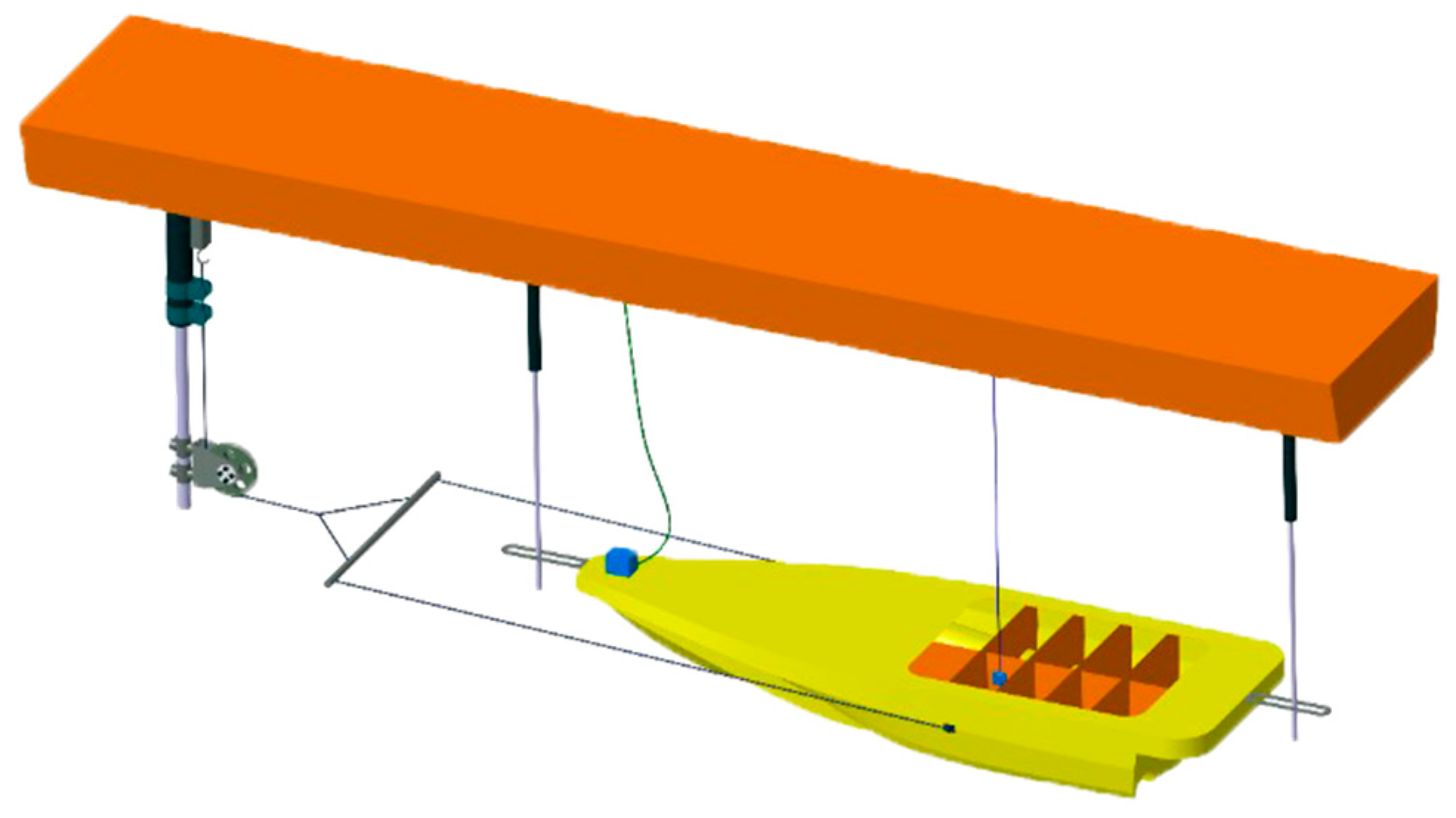
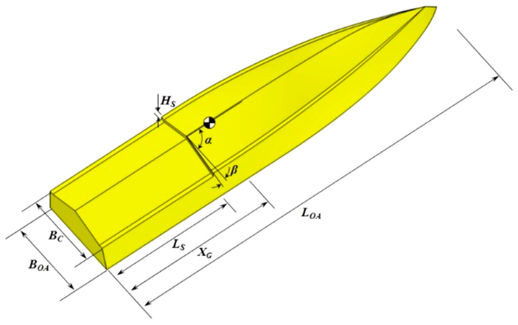
2.1. Model Introduction

According to the statistical results of the dimensions of existing planing boats by Taunton et al. [2,3], the length of a modern high-speed planing boat is usually 10-14 m. In considering the actual conditions, in this article the scale of the ratio between real boat and the model $\mathsf{\lambda }$ is selected as 5, and the total length of the hull is between 9 and 12 m. The real boat dimensions used for calculation and analysis are listed as the

Table 1. Main dimensions of main hull in real scale.

Symbol	Description	Value
$L_{OA}$	Length overall, m	10
$B_{OA}$	Beam, m	2.09
$D_{OA}$	Depth, m	1.35
$K_g$	Height of the gravity, m	0.75
$\mathsf{\theta }$	Trim angle in calm water, degree	1.05
$T_F$	Draft in middle of the boat, m	0.505
$T_A$	Draft in stern, m	0.597
$B_C$	Width of the chine, m	1.5
$L_s$	Longitudinal length of the step, m	3.11
$H_s$	Height of the step, m	0.1
$\mathsf{\alpha }$	The angle between step and longitudinal section in center plane, degree	90
$\mathsf{\beta }$	Dead risen angle, degree	20
$\Delta$	Displacement, T	3.75
$X_G$	Longitudinal center of gravity, m	3.5

.

The boat geometry is shown as Figure 1, the model is marked as SS700 and the weight is 20 kg. And the planing boat is Deep-V type mono-hull with step arranged in the middle of the boat.

2.2. Mathematical and Numerical Method

During simulation, the same mathematical and numerical method is applied as the investigation of the air-intake of the planing trimaran by Lei et al. [20], the governing equation of incompressible viscous flow is described by the Reynold Averaged Navier-Stokes Equations (RANSE) which is the most widely used method in engineering. The equation is described as follows:

$$\frac{\partial \overline{u_i}}{\partial \mathrm{t}}+\overline{u_j}\frac{\partial \overline{u_i}}{\partial x_j}+\frac{\partial }{\partial x_j}\left(\overline{u_i^{\prime }{u}_j^{\prime }}\right)=-\frac{1}{\rho }\frac{\partial \overline{p}}{\partial x_i}+v\frac{{\partial }^2\overline{u_i}}{\partial x_i\partial x_j}$$

(1)

where $\overline{u_i},\overline{u_j}$ denote the time averaged velocity components; $u_i^{\prime },u_j^{\prime }$ are the fluctuations of the velocity components; $\overline{p}$ is the time averaged pressure; $\mathsf{\rho }$ is dynamic viscosity coefficient; t is time; and $x_i, x_j$ are unit vectors in directions of i and j. To close this set of equations, the Shear Stress Transport (SST) turbulence model is used.

The transported variable of turbulent kinetic energy, k, is defined as follows:

$$\frac{\partial }{\partial t}\left(\rho k\right)+\frac{\partial }{\partial x_i}\left(\rho k{u}_i\right)=\frac{\partial }{\partial x_j}\left({\mathsf{\Gamma }}_k\frac{\partial k}{\partial x_j}\right)+G_k-Y_k$$

(2)

The second transported variable $\mathsf{\omega }$ is defined as follows:

$$\frac{\partial }{\partial t}\left(\rho \omega \right)+\frac{\partial }{\partial x_i}\left(\rho \omega u_i\right)=\frac{\partial }{\partial x_j}\left({\mathsf{\Gamma }}_{\omega }\frac{\partial \omega }{\partial x_j}\right)+G_{\omega }-Y_{\omega }+D_{\omega }$$

(3)

${\mathrm{G}}_k, G_{\omega }$ represent the turbulent kinetic energies due to the average velocity gradient; $Y_k, Y_{\omega }$ are turbulent dissipation terms; ${\mathsf{\Gamma }}_k, {\mathsf{\Gamma }}_{\omega }$ denote the effective diffusion terms; $D_{\omega }$ is the orthogonal divergence term.

The volume of fluid (VOF) model is applied to track the location and evolution of the free surface. The basic idea of the VOF is to define the marking function α in the discrete domain and to determine the value of the volume function in one grid according to the volume of the fluid in it: When the value of α is 1 or 0, there is only one fluid in the grid. When the value of α is between 0 and 1, it is occupied by two kinds of fluids, that means there is a free surface in the grid. α satisfies the following transport equation:

$$\frac{\partial \alpha }{\partial t}+u\frac{\partial \alpha }{\partial x}+v\frac{\partial \alpha }{\partial y}=0$$

(4)

Other than the solving process of traditional ships, the planing boat is mainly supported by the hydrodynamic lift during planing. The hull behavior (pitch and heave) at high speed is very different from that in static floating and has significant influence on the resistance performance. Therefore, a 6-DOF motion equation is introduced here as Figure 2 shown and the moment of hull body is implemented by the coupling of the motion and flow solver.

After the initial flow field solving, the force and moment acting on the hull body, including the shear stress, pressure caused by interaction of model and flow field and model gravity, could be acquired by the equations below:

$$\overrightarrow{F}={{\displaystyle \int }}_S^{}\left(\left[\tau \right]-p\left[I\right]\right)·\overrightarrow{n}dS$$

(5)

$$\overrightarrow{M}={{\displaystyle \int }}_s^{}\left(\overrightarrow{r}-\overrightarrow{r_G}\right)\left(\left[\tau \right]-p\left[I\right]\right)·\overrightarrow{n}dS$$

(6)

where $\left[\tau \right],p\left[I\right]$ are the shearing force and pressure respectively, $\left[I\right]$ is the unit vector of the pressure. $\overrightarrow{n}$ denotes the outer normal vector of the model surface, $\overrightarrow{r}$ and $\overrightarrow{r_G}$ stand for displacement of mesh nodes on hull surfaces and displacement of the gravity center. S represents the hull surfaces. The linear displacement $\overrightarrow{X}$ and angular displacement $\overrightarrow{\theta }$ can be calculated by using

$$\overrightarrow{F}=m\frac{d^2\overrightarrow{X}}{d{t}^2}$$

(7)

$$\overrightarrow{M}=\frac{d}{dt}\left(I\frac{d\overrightarrow{\theta }}{dt}\right)$$

(8)

where $\overrightarrow{F}$ and $\overrightarrow{M}$ are defined as the force and moment vector acting on the model, m denotes the mass.

After solving the initial mesh, pressure and shear stress field around hull body are acquired and the total force and the moment can be calculated by integrating them on hull surface according to Equations (5) and (6). Using Equations (7) and (8), the hull displacement is solved and the hull motion is subsequently modelled through the mesh node moving to a new position. The next iteration of flow solver is carried out on the new mesh. When the variations of calculated forces and moments approach zero, the hull body is considered to have achieved the balance state and the calculation process is terminated.

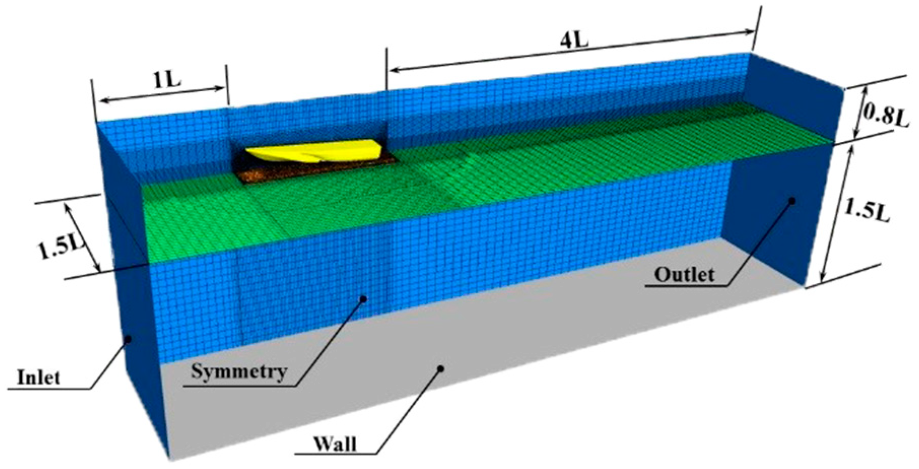
2.3. Domain Codition and Boundary Conditions

The simulated domain and boundary conditions are specified in Figure 3. Due to the flow field being axially symmetric with the hull, modeling the half hull body is satisfy the simulation work. In the boundary condition setting, the hull body is a rigid moving body and no-slip phenomenon on the hull surface. The free-slip condition is applied on the top, side and bottom boundaries. The center plane of hull body is set as symmetry plane. The flow velocity at inlet is defined as the tested speed and the pressure outlet is filled as hydrostatic pressure which is expressed as a function of water level height. Furthermore, the initial location of the free surface is determined by defining the volume fraction function of water and air at the inlet and outlet.

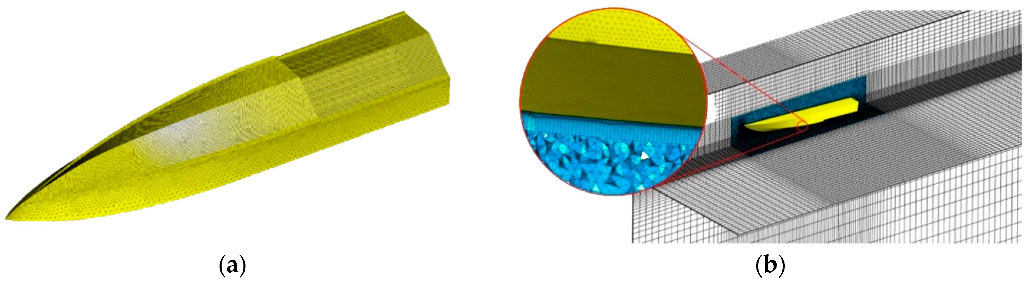
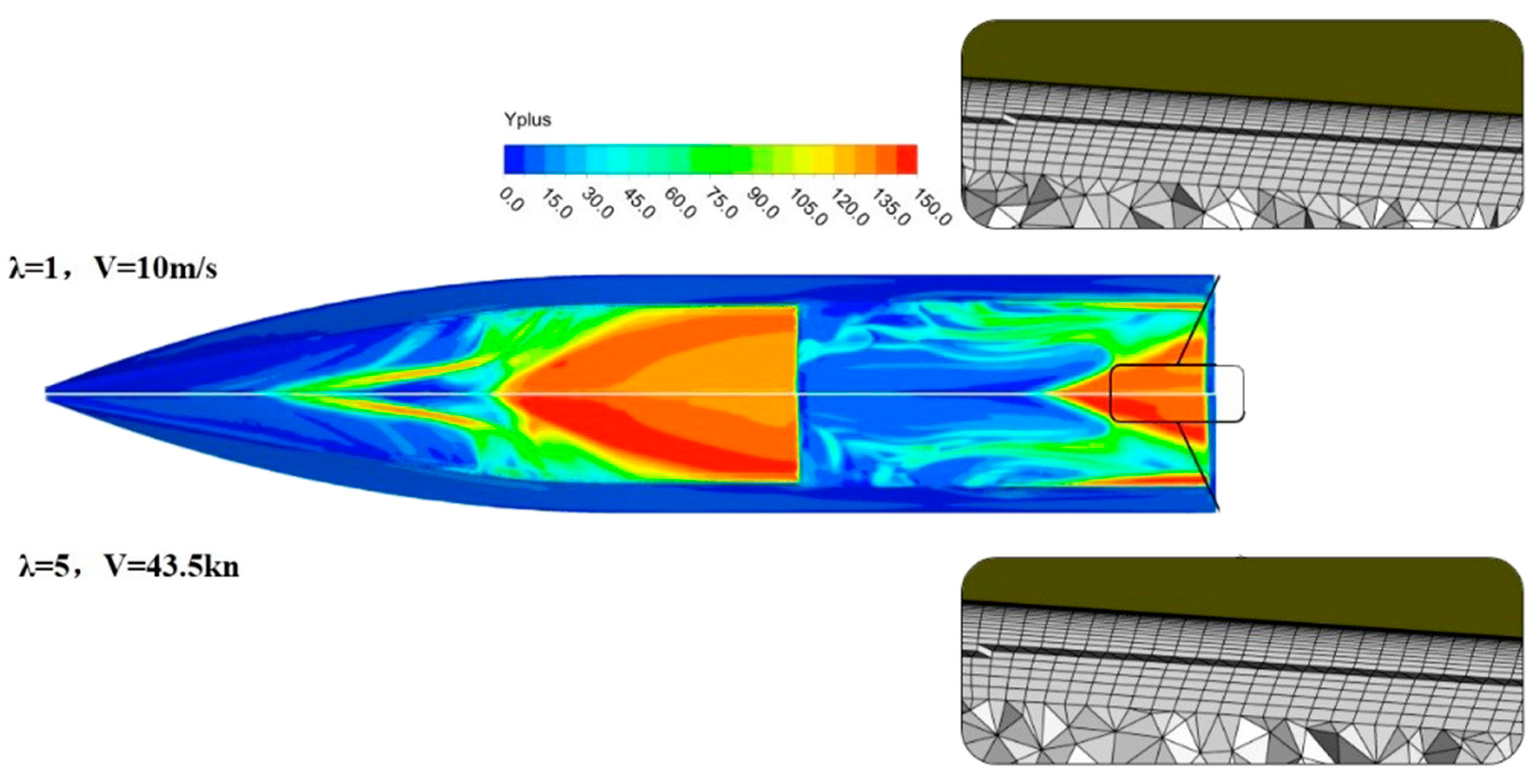
2.4. Mesh Generation

The mesh generation in this study is accomplished by using ANSYS ICEM, as shown in Figure 4, the calculation domain is discretized in using of structured and unstructured meshes. A mesh with triangular elements is generated on the hull surface, especially, refinement adopted on the main flow fields such as planing surfaces and nearby the steps; the 10 boundary layers are refined with prism elements created through extending the surface mesh node; the region around the boat is filled with tetrahedral elements, while in the far field, a structured mesh with hexahedral elements is generated to reduce the number of elements.

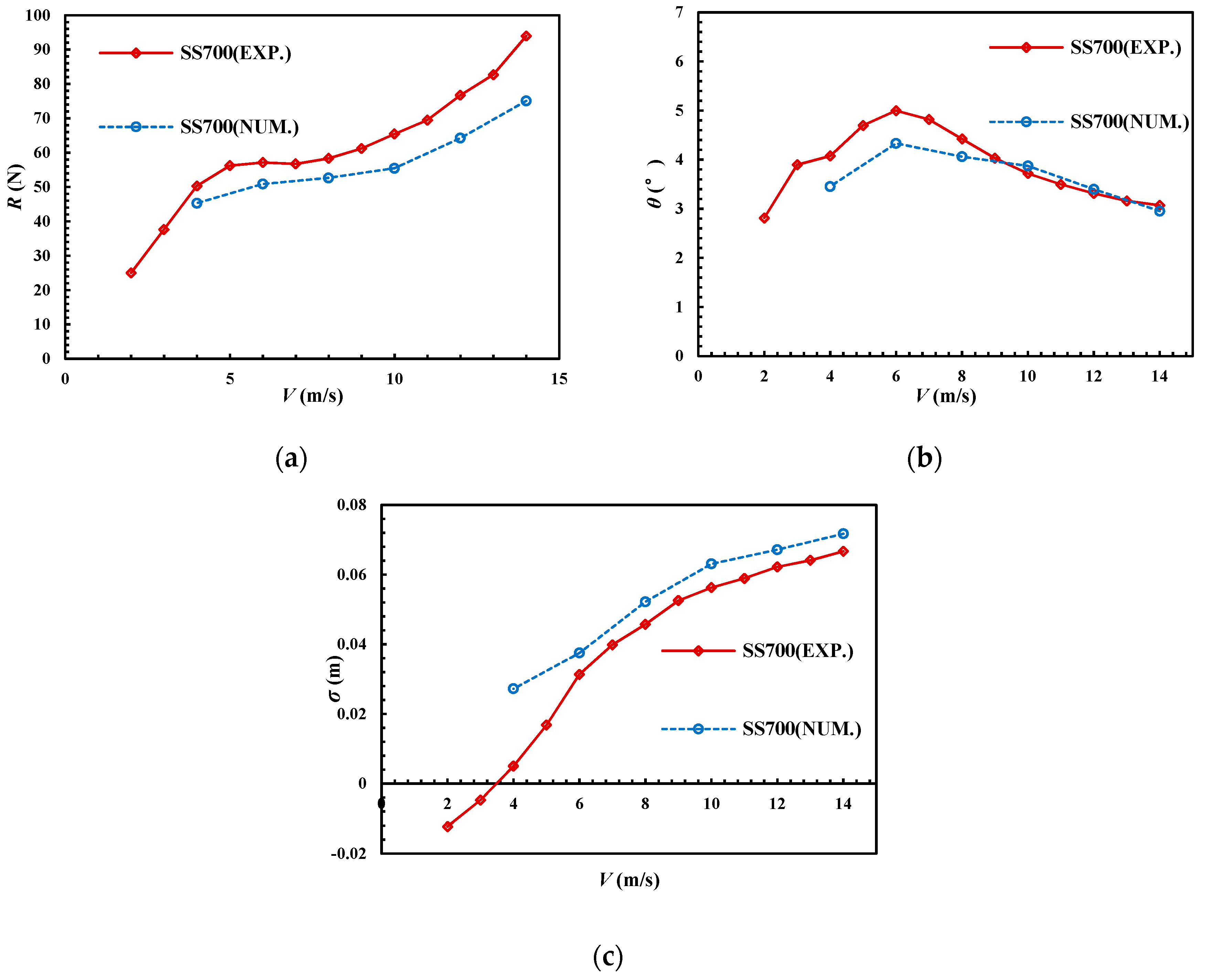
2.5. Validation and Verification

To verify and validate the numerical method, the comparison of calculation and experimental date has been studied. The towing test has been carried out in the towing tank of the China Special Vehicle Research Institute, and its dimensions are 510 m × 6.5 m × 6.8 m in length, width, and depth, respectively, the max towing speed is 22 m/s.

The towing test model (SS700) has the same geometric characteristics as the model. The model has been polished and painted before the test in order to ensure the smoothness of the surface. As Figure 5 shows, the model is driven by a carriage platform and has only two degrees of freedom (heave and pitch). The measured records are resistance, trim angle, and heave, detected by a dynamometer, electronic angle sensor, and cable-extension displacement sensor, respectively.

The results are listed as

Table 2. Computational result and experimental data.

V m/s	R(N)			Trim (deg)			Sinkage(m)
	Computation	Experiment	Error (%)	Computation	Experiment	Error (%)	Computation	Experiment	Error (%)
4	45.299	50.306	9.95	3.455	4.075	15.23	0.027	0.005	445.40
6	50.89	57.143	10.94	4.332	4.999	13.35	0.038	0.031	19.66
8	52.66	58.340	9.74	4.062	4.422	8.15	0.052	0.046	14.16
10	55.459	65.452	15.27	3.873	3.718	4.18	0.063	0.056	12.10
12	64.247	76.724	16.26	3.398	3.312	2.60	0.067	0.062	7.94
14	75.076	93.970	20.11	2.953	3.07	3.80	0.072	0.067	7.53

and Figure 6,

As the simulation, the compared speed range selected from 4–14 m/s due to the obvious porpoising observed when the speed is over 14 m/s. Generally, the trends of resistance and trim angle of calculation agree well with the experimental date, and the average errors are 11.21%, 7.89% respectively. However, the sinkage calculated is quadruple that of the experimental result at 2 m/s, while in fact the value difference is only 0.022 m; it can also be observed that the experiment data is larger than calculated, mainly because the numerical method adopted in this study is not sufficient to capture the spatter that acts on the hull and, therefore, the corresponding friction resistance cannot be accounted for.

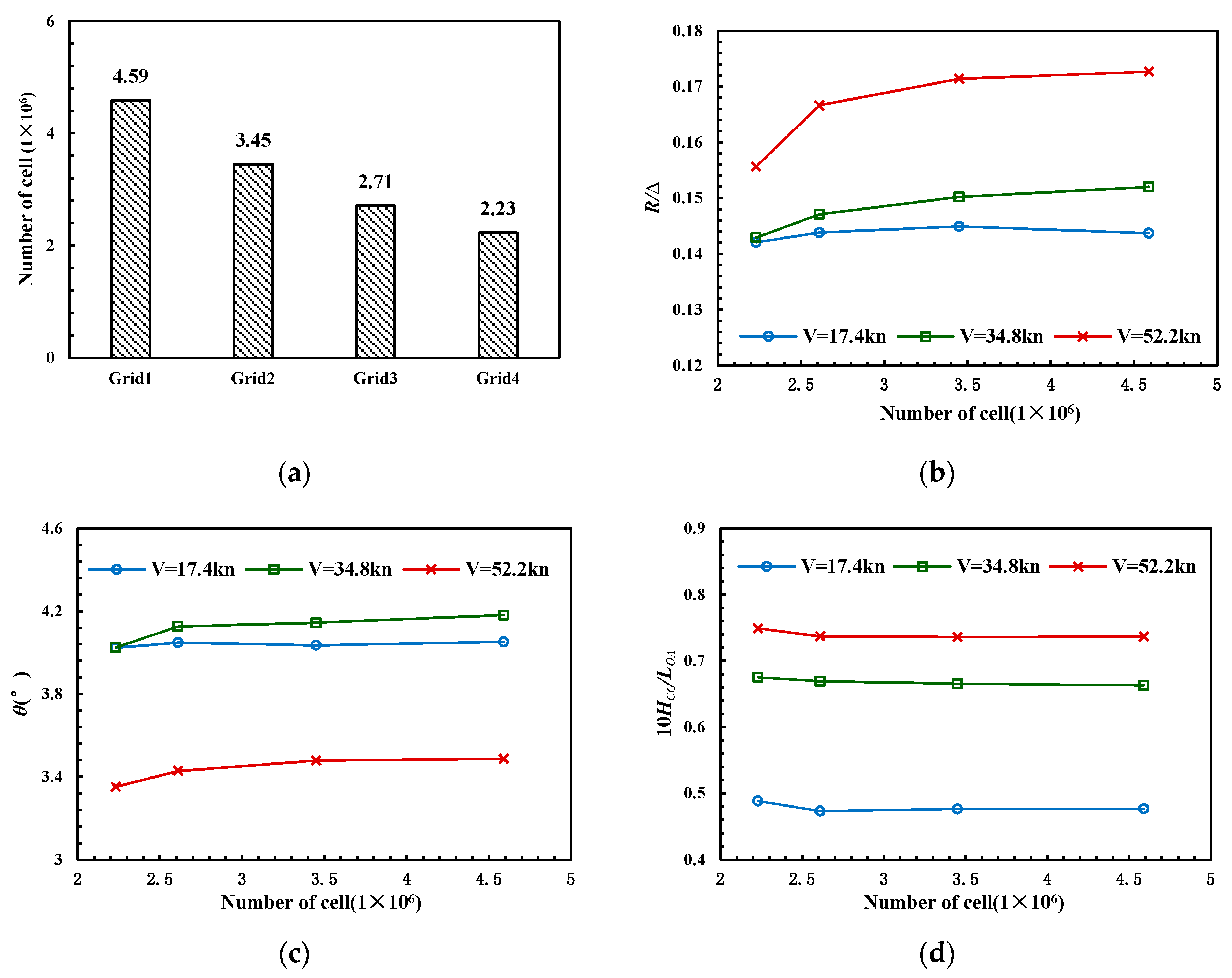
2.6. Generation Convergence of the Full-Scaled Model

The key point in analysis of the full-scaled boat is to establish numerical calculation with capturing the hydrodynamic characteristics accurately. Therefore, it is necessary to extend the numerical solution of the flow field around the model to the full-scaled boat. The domain built for the full-scaled boat is amplified from the model and the capacity is ${\lambda }^3$ times larger than the original model. However, if using the mesh size of the original model in discretizing, the number of total meshes increases geometrically in corresponding. Furthermore, the difficulty and time consumption of the calculation are increased. In considering of the accuracies of model calculation and flow field description, the mesh size of the full-scaled boat can be selected according to the model.

Furthermore, there is a difference in Reynolds number between the model and the full-scaled boat during sailing, at the same Froude number, the Reynolds number of full-scaled boat is ${\lambda }^{3/2}$ times that of the model’s. The refinement is carried out in region of boundary layer to ensure the agreement of the value of y+. The capture conditions of the boundary layer grid in two dimensions are investigated through velocity distribution in section of X/L = 0.4 and velocity versus distance from wall as the Figure 7 and Figure 8 shown. $V/V_{max}$ represents the ratios of the velocity with the velocity of the flow in turbulent core region. It can be seen that the method used in this paper can still simulate the velocity transition from the viscous bottom layer to the turbulent core region on the full-scaled boat, which can meet the needs of the numerical simulation of the flow around the full-scaled boat.

And the mesh convergence studies are carried out at the volume-based Froude numbers of 2.29, 4.58, and 6.87. Four sets mesh of sizes, named as Grid1–Grid4, are investigated, the original size and three others with mesh fineness $\sqrt{2}$, 2 and $2\sqrt{2}$ respectively. The total numbers of the meshes are shown in Figure 9. The results are also compared in Figure 9 and

Table 3. Mesh generation strategy and mesh convergence.

%	$\mathbf{R}/\Delta$			$\mathsf{\theta }$			$10 {\mathit{H}}_{\mathit{C}\mathit{G}}/{\mathit{L}}_{\mathit{O}\mathit{A}}$
	17.4kn	34.8kn	52.2kn	17.4kn	34.8kn	52.2kn	17.4kn	34.8kn	52.2kn
$\frac{G3-G4}{G4}$	7.0572	2.9371	1.2342	2.2887	2.4969	0.5843	1.5902	0.8888	3.1325
$\frac{G2-G3}{G3}$	2.8512	2.1234	0.7768	1.4600	0.4514	0.3205	0.1282	0.5493	0.6850
$\frac{G1-G2}{G2}$	0.7407	1.1961	0.8402	0.2532	0.4147	0.4060	0.0509	0.3539	0.0409

$\mathrm{G}1-\mathrm{G}4$ denote the four refinements of the mesh generation strategy.

, of which the non-dimensional resistance is defined by the ratio of the resistance to hull weight (R/Δ) and the non-dimensional sinkage is defined as the ratio of the height of gravity to length of boat (10$H_{CG}/L_{OA}$). The volume-based Froude number $F_{r_{\nabla }}$ is chosen to represent the towing speed.

It can be seen that the calculation difference caused by mesh accuracy is no longer obvious when the mesh fineness beyond Grid2. In considering of the time consumption, the relative mesh size can be adopted in the full-scaled boat if the reduced scale is less, however, the boundary layer area should be refined.

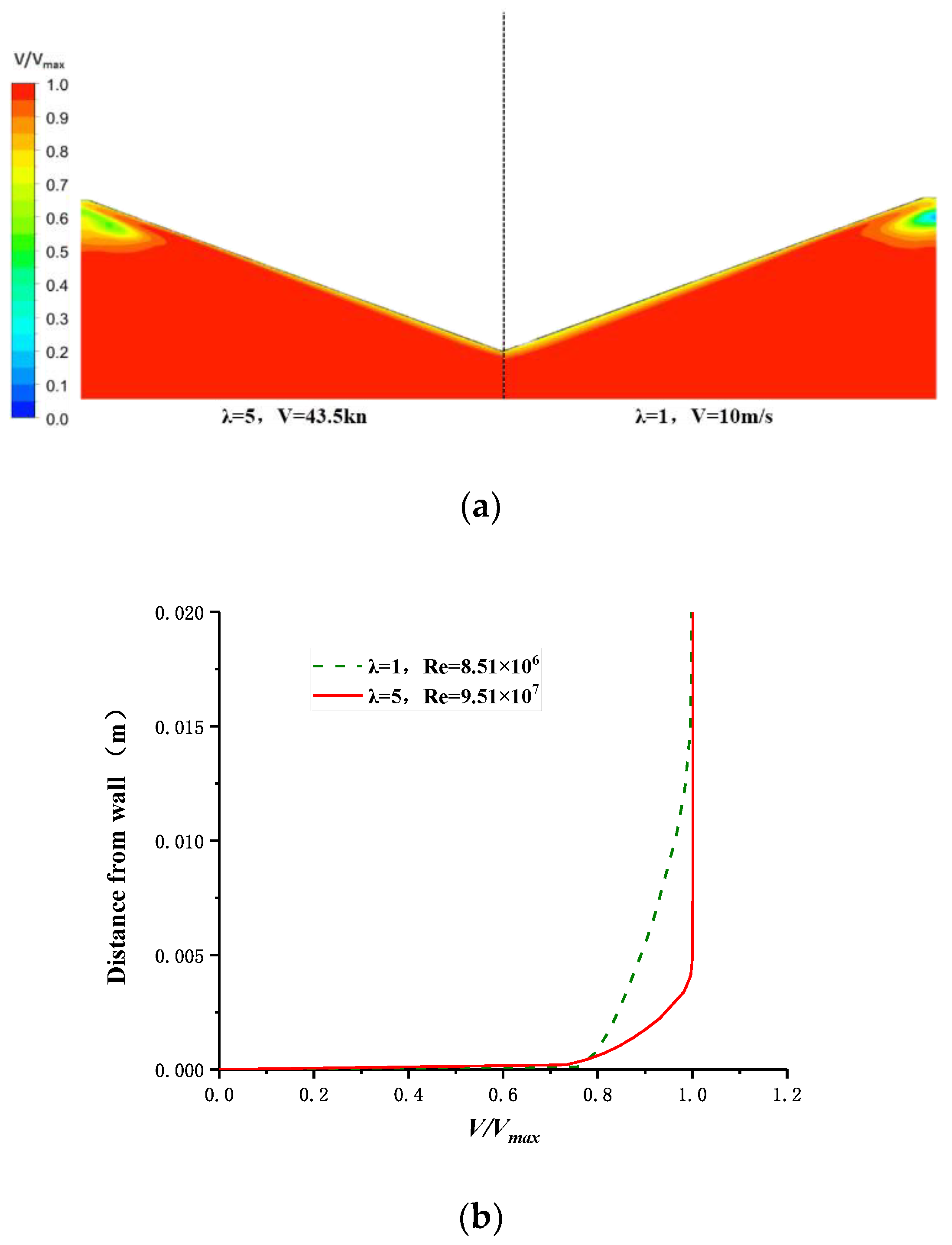
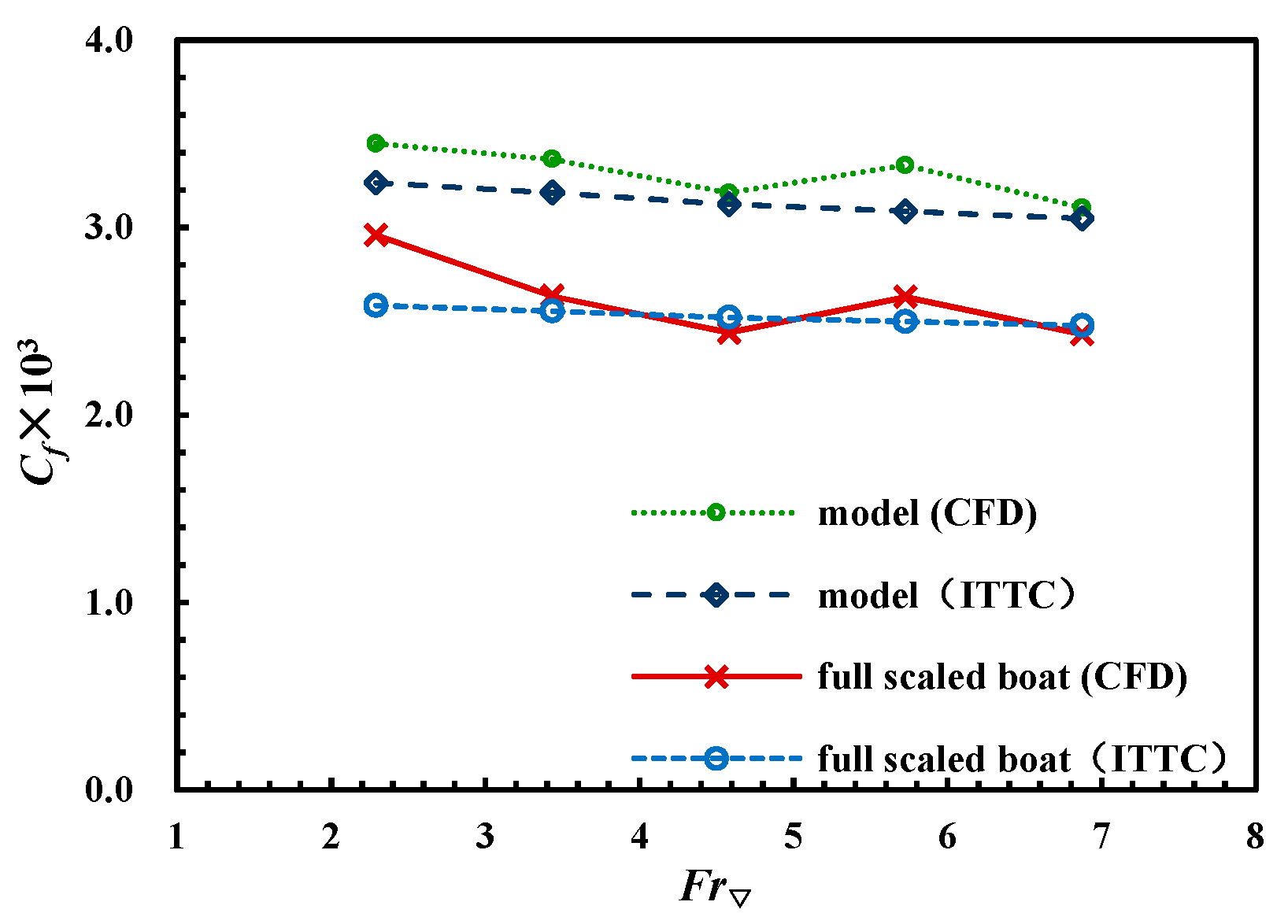
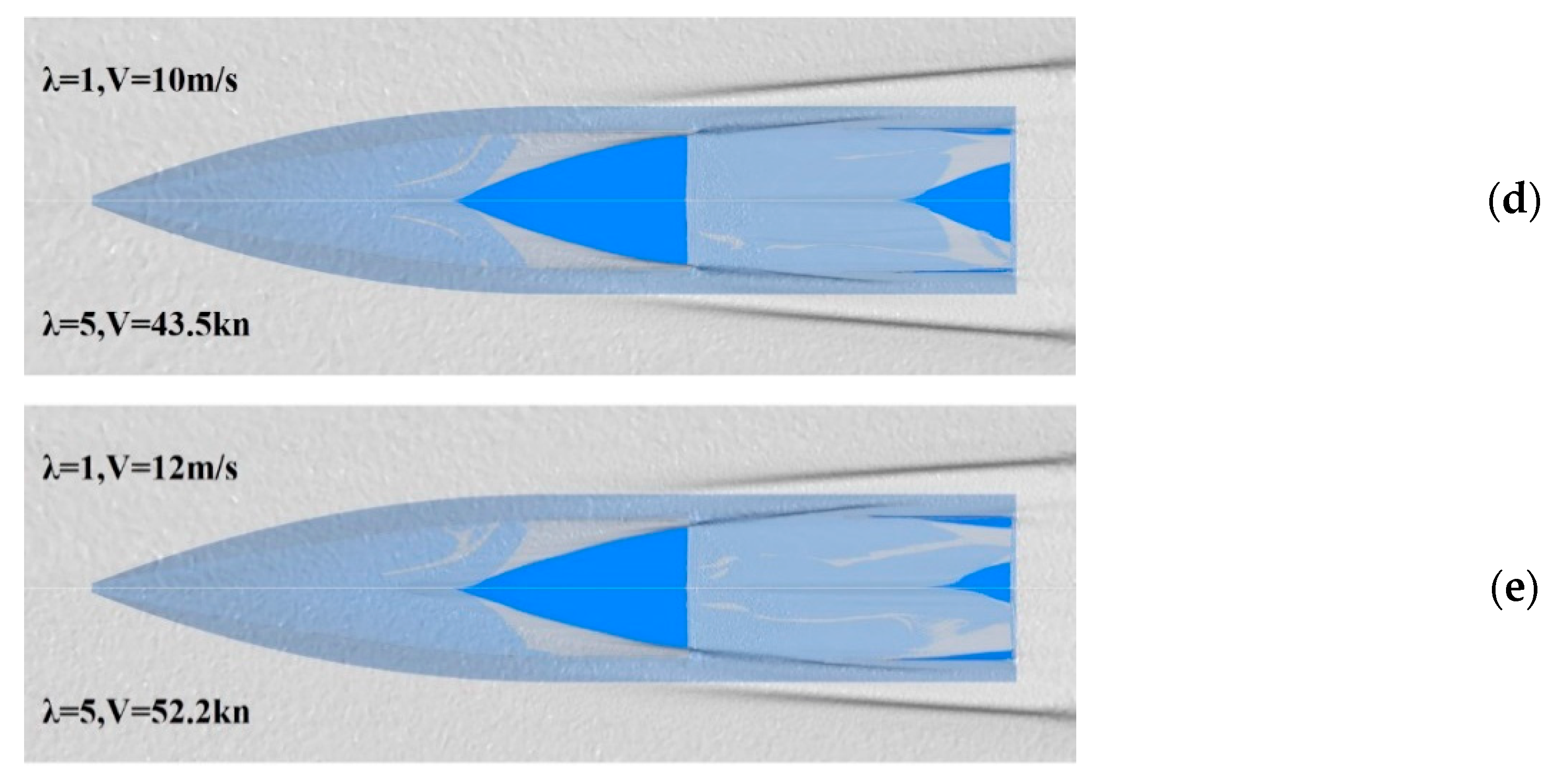
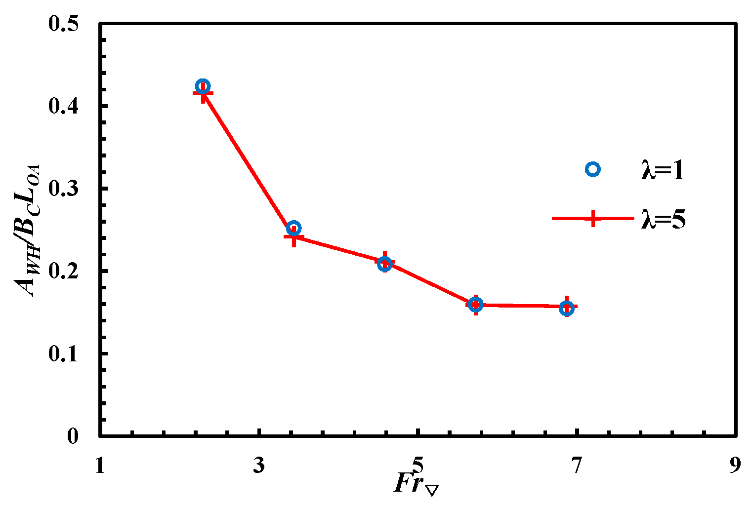
3. Scale Effect Analysis

The total resistance $R_t$ consists of residuary $R_r$ and friction $R_f$ resistance, derived in dimensionless form as follows:

$$R_t=R_r+R_f=C_r\times \frac{1}{2}\rho V^{2}S+C_f\times \frac{1}{2}\rho V^{2}S=C_t\times \frac{1}{2}\rho V^{2}S$$

(9)

$$C_t=C_r+C_f$$

(10)

$C_t$, $C_r$, and $C_f$ denote the total, residuary and friction resistance coefficient, respectively; furthermore, the residuary resistance is consisted of viscous pressure resistance and wave resistance. To analyse the scale effect clearly, hereby, the resistance is discussed in two parts: residuary and friction resistance.

As the mentioned above, the residuary resistance can be broken up into two parts, wave and viscous resistance. The wave resistance needs to be studied due to the proportion of wave resistance in total resistance of planing boat being up to 40%–50%, compared to a traditional ship. The similarity of waves between the different scaled planing boats including: one is flow after the step, and another is the wave beside of the hull.

As the Froude’s similarity, to the different dimensions of the geosim boats, if keeps the wave same, the wave resistance coefficient $C_w$,

$$C_w=R_w/0.5\rho V^2{A}_w$$

(11)

only related to the Froude number, $R_w$ is the wave resistance and $A_w$ is water plane area. Therefore, the simulations of model and full-scaled boat in the same Froude number were investigated.

As Figure 10 shows, the distributions of the bottom wave characteristics between the model (upper half figure) and full-scaled boat (lower half figure) are compared during the same volume Froude numbers. The lines of stagnation points on the model and boat both have similar contours in bow and stern, by the increase in the speed, the growth rates of the cavities after step also keep pace with each other. The boats with different dimensions show similar wetting surfaces on each planing surface, which means they have geometric similarities in wetting surface when the Froude number is the same.

In Figure 11, the area of wetting surface divided by the product of chine width with length of boat is used to eliminate the differences caused by different scales, the result also shows the similarity. Furthermore, the flow and the sections of wave cut around the hull side in two locations: $X/L_{OA}=0, 0.3$ of the different scales models during five speeds have been traced out in Figure 12, the similarity also can be observed.

The non-dimensional values in vertical and transverse are defined by the ratios of the chine width ($Z/B, X/B$). At same Froude number, the discrete points of the wave pattern are distributed along the hull basically, the wave heights difference between model and full-scaled boat are slight that means the deviation in wave energy is almost zero.

Otherwise, to the viscous pressure resistance, the pressure caused by the wave in a longitudinal direction can be ignored due to the wavelength being much larger than the length of boat when the stepped boat is planing, and as Figure 13 shows, the bottom pressure distribution which is relevant to the wave generation directly is studied in transverse orientation. The pressure coefficients on the keel in different speeds are plotted, and defined as

$$C_p=P/\frac{1}{2}\rho V^2$$

(12)

It shows good agreement in pressure distributions between the model and the full-scaled boat, and as the definition of the pressure coefficient, the pressure acting on the full-scaled boat is $\mathsf{\lambda }$ times larger than the model at the same one point.

Summarizing the discussion of the wave characteristics above, during the same Froude number, the lines of stationary points on the planing surface (shapes of wetted surface), forms of the air cavity, and the wave along the hull both reveal the geometric similarity. The residuary coefficients $C_r$ of different scaled models are compared in Figure 14, the max deviation is 6.02% occurring at the high speed region ($F{r}_{\nabla }=6.87$) which has a rapid decrease in the proportion of the residual resistance in total resistance, it can be considered that the computation conforms to the Froude’s similarity.

As for the friction resistance, the coefficient of friction resistance only depends on the Reynolds number $R_e$ and has no relation to the dimensions of the geosim boats as the Reynolds’s similarity. However, in comparison, the dimension of the model is much smaller than the full-scaled boat, and the towing speed is also slowed down to fulfill the Reynolds’s similarity, as a result there are differences in friction resistance.

Under the 1957 ITTC formula, the friction resistance coefficient can be obtained by

$$C_f=\frac{0.075}{{\left(\lg R_e-2\right)}^2}$$

(13)

The calculation process of the friction resistance coefficients is listed in

Table 4. The friction resistance coefficients based on two-dimensional method.

(1)	(2)	(3)	(4)	(5)	(6)	(7)	(8)
${\mathit{V}}_{\mathit{m}}/ \mathbf{m}/\mathbf{s}$	${\mathit{l}}_{\mathit{w}\mathit{f}\mathit{m}}/ \mathbf{m}$	${\mathit{l}}_{\mathit{w}\mathit{a}\mathit{m}}/ \mathbf{m}$	$\mathit{R}{\mathit{e}}_{\mathit{m}}$	${\mathit{C}}_{\mathit{f}\mathit{m}}$	${\mathit{V}}_{\mathit{s}}/ \mathbf{m}/\mathbf{s}$	$\mathit{R}{\mathit{e}}_{\mathit{s}}$	${\mathit{C}}_{\mathit{f}\mathit{s}}+\Delta {\mathit{C}}_{\mathit{f}}$
			$\frac{\left(1\right)\times \left(\left(2\right)+\left(3\right)\right)}{0.8731\times {10}^{-6}}$	As Eq. (13)	$\left(1\right)\times \sqrt{\mathit{\lambda }}$	$\frac{\left(1\right)\times \mathit{\lambda }\times \left(\left(2\right)+\left(3\right)\right)}{0.8731\times {10}^{-6}}$	As Eq. (13)
4	0.832	0.584	6.49 × 106	3.24 × 10−3	8.94	7.25 × 107	2.58 × 10−3
6	0.610	0.426	7.12 × 106	3.19 × 10−3	13.42	7.96 × 107	2.55 × 10−3
8	0.550	0.317	7.94× 106	3.12 × 10−3	17.89	8.87 × 107	2.52 × 10−3
10	0.501	0.242	8.51 × 106	3.09 × 10−3	22.36	9.51 × 107	2.50 × 10−3
12	0.482	0.183	9.14 × 106	3.05 × 10−3	26.83	1.02 × 108	2.48 × 10−3

, subscripts m and s are for model and full-scaled boat components respectively. $V_m, V_s$ denote the velocity of the model and the full-scaled boat; $l_{wfm}$ stands for the wetted length of the fore body; and $l_{wam}$ is wetted length of aft body. It can be seen that, as speed increases, more hull body is lifted out from the water and the air cavity behind the step is enlarged, which makes the wetted length on both fore and aft body decrease. $R_e$ is the Reynolds number and 0.8731 × 10⁻⁶ is dynamic viscosity coefficient of water in Celsius temperature of 25.

As Figure 15 shows, compared to the calculated data by ITTC formula, the CFD calculations of the models are increased by 4.77% on average, and the calculations of boats also added 3.57%, indeed, the difference is decreased by the dimension raise up. As the speed range selected, the CFD simulated friction resistance coefficients of boat are decreased by 0.67 × 10⁻³ than model on average, and the ITTC results are also cut down 0.61 × 10⁻³ between boat and model. It means the scale effect can be predicted during the simulation of the full-scaled boat, however, the effect is larger than ITTC general concludes.

As discussed above, the residuary resistance coefficients in different scales are approximately equal, and the friction resistance coefficients show the scale effect, this conclusion means it is valid to predict the full-scaled boat performance and behavior by model information. The total resistance coefficient of the boat also can be obtained by the two-dimensional method as follows:

$$C_{rm}=C_{tm}-C_{fm}$$

(14)

$$C_{ts}=C_{rs}+C_{fs}+\Delta C_f=C_{fs}+\left(C_{tm}-C_{fm}\right)+\Delta C_f$$

(15)

$\Delta C_f$ In addition, it is different from the conventional displacement ship, the proportion of air resistance $R_A$ in total resistance is much higher. The ratios of the air and total resistance in model and boat computation are listed as Figure 16, the proportion of the air resistance in total drag is only 0.5% during the low velocity ($F_{r_{\nabla }}=2.29$), however by the speed increasing, the proportion of air resistance is also raised up rapidly. The maximum ratios of the model and boat are 6.9% and 8.6%, respectively ($F_{r_{\nabla }}=6.87$). Deviation will be added into the calculations of the residuary resistance coefficient if air resistance is classified into residuary resistance due to the similarity of Froude not being satisfied between the air flows around the model and the boat. To make the dimension difference explicitly, the air resistance will be subtracted from the total resistance and marked with $R_t^{\prime }$.

The calculated process and results of the total resistance are recorded as

Table 5. Full-scale resistance calculation table based on calculated model resistance and two-dimensional method.

(9)	(10)	(11)	(12)	(13)	(14)	(15)	(16)	(17)
${\mathit{A}}_{\mathit{w}\mathit{m}}$	${\mathit{R}}_{\mathit{f}\mathit{m}}$	${\mathit{R}}_{\mathit{t}\mathit{m}}^{\prime }$	${\mathit{c}}_{\mathit{t}\mathit{m}}$	${\mathit{c}}_{\mathit{r}\mathit{m}}$	${\mathit{c}}_{\mathit{t}\mathit{s}}$	${\mathit{A}}_{\mathit{w}\mathit{s}}$	${\mathit{R}}_{\mathit{t}\mathit{s}}^{\prime }$	${\mathit{R}}_{\mathit{t}\mathit{s}}-{\mathit{R}}_{\mathit{a}\mathit{s}}$
	As Eq. (4)		As Eq. (10)	(12) − (5)	(13) + (8)	$\left(9\right)\times {\mathit{\lambda }}^2$	As Eq. (10)
0.509	13.16	44.91	1.11 × 10−2	7.82 × 10−3	1.04 × 10−3	12.72	5.28	5.32
0.302	17.29	48.08	8.86 × 10−3	5.67 × 10−3	8.22× 10−3	7.56	5.58	5.44
0.250	24.98	47.78	5.98 × 10−3	2.85 × 10−3	5.37 × 10−3	6.26	5.37	5.29
0.192	29.49	48.92	5.12 × 10−3	2.03 × 10−3	4.53 × 10−3	4.79	5.41	5.24
0.186	40.69	55.38	4.15 × 10−3	1.10 × 10−3	3.58 × 10−3	4.65	5.97	5.76

${\mathrm{R}}_{\mathrm{ts}}-{\mathrm{R}}_{\mathrm{as}}$ denotes the resistance deducted the air resistance from the calculated total resistance of a real boat.

, $A_w$ stands for the area of the water plane.

In summary, the total resistances of the boat by simulating in CFD and calculating in the two-dimensional method are compared in Figure 17. The trends of drag revealed by two methods are in accordance with each other, however, the resistance calculated by CFD is higher than the two-dimensional method due to the influence of the scaled effect by numerical method being greater, during the speed range, and the average deviation is 1.97%.

Otherwise, the obvious porpoising occurrence is also observed when the Froude number is beyond 8.02, in view of the hydrodynamic characteristics similarity, the stabilization of longitudinal motion should be studied. As Figure 18 shows, the trim angles and resistances of boat and model are plotted as functions of oscillation period, the average resistances are 41% and 43% of average oscillation amplitude, trim angles are 1.2° and 1.19°, respectively.

The similarity also can be explored in the stabilization of longitudinal motion, furthermore, the scale effect reflected in the period deviation. The calculated boat oscillation period $T_s$ is 0.678 s and the model period $T_m$ is 0.3s, the ration of them is the square root of the scales ($T_s/T_m=\sqrt{\lambda }$), that is exactly the scales effect magnified the period of the hull oscillation.

4. Conclusion

In this paper the geosim models with different dimensions are discussed, and the point is to study the effect of the scale. Based on the experimental data, the numerical method has been verified and validated, the following conclusions can be drawn:

1. The numerical method used here is credible for the simulation of a planing boat. The advantage is mainly reflected in the modelling of hull motion, which is implemented by the coupling iterative solving of the governing and motion equations. Therefore, it is not necessary to estimate the hull position before solving flow field, and the dependence on experimental data is weakened. The reasonability of the CFD method in performance prediction is verified by towing tank test already, the differences investigated in different scaled models are receivable.

2. As the calculation, the scale effect which complied with the similarity of Renault is revealed, the similarity of the wave pattern and pressure distribution which complied with Froude’s similarity also observed, and the total resistance calculated also closes to the result obtained by the two-dimensional method.

3. The scales effect in longitudinal steadiness is captured in periods of the porpoising occurrence. The ratio value of the full-scaled boat oscillation period and the model is the square root of the scales.

References

1. Lee, E.; Pavkov, M.; Mccueweil, L. The Systematic Variation of Step Configuration and Displacement for a Double-step Planing Craft. J. Ship Prod. Des. 2014, 30, 89–97. [Google Scholar] [CrossRef]
2. Taunton, D.J.; Hudson, D.A.; Shenoi, R.A. Characteristics of a series of high speed hard chine planing hulls-Part 1: Performance in calm water. Int. J. Small Craft Technol. 2010, 152, 55–75. [Google Scholar] [CrossRef]
3. Taunton, D.J.; Hudson, D.A.; Shenoi, R.A. Characteristics of a series of high speed hard chine planing hulls-Part II: Performance in waves. Int. J. Small Craft Technol. 2011, 152, 55–75. [Google Scholar] [CrossRef]
4. Jiang, Y.; Sun, H.B.; Zou, J.; Hu, A.K.; Yang, J.L. Analysis of tunnel hydrodynamic characteristics for planing trimaran by model tests and numerical simulations. Ocean Eng. 2016, 113, 101–110. [Google Scholar] [CrossRef]
5. Savander, B.R.; Scorpio, S.M.; Taylor, R.K. Steady Hydrodynamic Analysis of Planing Surfaces. J. Ship Res. 2002, 46, 248–279. [Google Scholar] [CrossRef]
6. Ghassemi, H.; Ghiasi, M. A combined method for the hydrodynamic characteristics of planing crafts. Ocean Eng. 2015, 35, 310–322. [Google Scholar] [CrossRef]
7. Pemberton, R.; Turnock, S.; Watson, S. Free surface CFD simulations of the flow around a planing plate. In Proceedings of the 6th International Conference on Fast Sea Transportation (FAST), Southampton, UK, 1 January 2001. [Google Scholar]
8. Subramanian, V.A.; Subramanyam, P.V.V. Effect of tunnel on the resistance of high-speed planing craft. J. Nav. Archit. Mar. Eng. 2009, 2, 15–26. [Google Scholar] [CrossRef]
9. Subramanian, V.A.; Subramanyam, P.V.V.; Ali, N.S. Pressure and drag influences due to tunnels in high-speed planing craft. Int. Shipbuild. Prog. 2007, 1, 25–44. [Google Scholar]
10. Azcueta, R. RANSE Simulations for Sailing Yachts Including Dynamic Sinkage & Trim and Unsteady Motions in Waves. In Proceedings of the High Performance Yacht Design Conference, Auckland, New Zealand, 1 January 2002. [Google Scholar]
11. Shengcheng, J.I.; Ouahsine, A.; Smaoui, H.; Sergent, P. 3D Modeling of sediment movement by ships-generated wakes in confined shipping channel. Int. J. Sediment Res. 2014, 29, 49–58. [Google Scholar] [CrossRef]
12. Linde, F.; Ouahsine, A.; Huybrechts, N.; Sergent, P. Three-dimensional numerical simulation of ship resistance in restricted waterways: Effect of ship sinkage and channel restriction. J. Waterw. Port. Coast. Ocean Eng. 2017, 143, 06016003. [Google Scholar] [CrossRef]
13. Yousefi, R.; Shifaghat, R.; Shakeri, M. Hydrodynamic analysis techniques for high-speed planing hulls. Appl. Ocean Res. 2013, 42, 105–113. [Google Scholar] [CrossRef]
14. Azcueta, R.; Rousselon, N. CFD Applied to Super and Mega Yacht Design. In Proceedings of the Design, Construction and Operation of Super and Mega Yachts Conference, Genova, Italy, 10 April 2009. [Google Scholar]
15. Lotfi, P.; Ashrafizaadeh, M.; Esfahan, R.K. Numerical investigation of a stepped planing hull in calm water. Ocean Eng. 2015, 94, 103–110. [Google Scholar] [CrossRef]
16. Du, P.; Ouahsine, A.; Sergent, P. Influence of the draft to ship dynamics in the virtual tank based on openfoam. In Proceedings of the 7th International Conference on Computational Methods in Marine Engineering (MARINE 2017), Nantes, France, 15 May 2017. [Google Scholar]
17. Hochkirch, K.; Mallol, B. On the importance of full-scale CFD simulations for ships. In Proceedings of the 12th International Conference on Computer Applications and Information Technology in the Maritime Industries (COMPIT 2013), Cortona, Italy, 9 May 2013. [Google Scholar]
18. Starke, B. The prediction of scale effects on ship wave systems using a steady iterative RANS method. In Proceedings of the 7th Numerical Towing Tank Symposium, Hamburg, Germany, 3–5 October 2004. [Google Scholar]
19. Dubrovsky, V.A.; Matveev, K.I. Small waterplane area ship models: Re-analysis of test results based on scale effect and form drag. Ocean Eng. 2006, 33, 950–963. [Google Scholar] [CrossRef]
20. Lei, D.; Hanbing, S.; Yi, J.; Ping, L. Numerical research on the resistance reduction of air intake. Water 2019, 11, 280. [Google Scholar] [CrossRef]
Figure 1. Single stepped planing hull in Taunton series.
Jmse 07 00392 g001
Figure 2. Local coordinate system of planing hull motion solver.
Jmse 07 00392 g002
Figure 3. Calculation domain.
Jmse 07 00392 g003
Figure 4. Mesh generation and refinement: (a) Bottom plan; (b) Domain and boundary layers.
Jmse 07 00392 g004
Figure 5. Test plan.
Jmse 07 00392 g005
Figure 6. Mesh generation strategy and mesh convergence study for full scale numerical simulation: (a) Resistance; (b) Trim angle; (c) Sinkage.
Jmse 07 00392 g006
Figure 7. Y+ distribution and boundary layer mesh in both model and real scale.
Jmse 07 00392 g007
Figure 8. Velocity distribution in section of X/L = 0.4 and velocity versus distance from wall: (a) Velocity distribution in section of X/L = 0.4; (b) velocity versus distance from wall.
Jmse 07 00392 g008
Figure 9. Mesh generation strategy and mesh convergence study for full-scaled numerical simulation: (a) Total number of grids; (b) Resistance; (c) Trim angle; (d) Sinkage.
Jmse 07 00392 g009
Figure 10. Bottom view of wave characteristics of stepped planing hull in both model and full-scaled boat: (a) F r = 2.29 ; (b) F r = 3.34 ; (c) F r = 4..58 ; (d) F r = 5.73 ; (e) F r = 6.87 .
Jmse 07 00392 g010aJmse 07 00392 g010b
Figure 11. Non-dimensional wetted area.
Jmse 07 00392 g011
Figure 12. The Flow and the transverse wave pattern of stepped planing hull in both model and full-scaled boat: (a,f) F r = 2.29 ; (b,g) F r = 3.34 ; (c,h) F r = 4.58 ; (d,h) F r = 5.73 ; (e,j) F r = 6.87 .
Jmse 07 00392 g012aJmse 07 00392 g012bJmse 07 00392 g012c
Figure 13. Pressure coefficient distribution on the keel line: (a) F r = 2.29 ; (b) F r = 3.34 ; (c) F r = 4..58 ; (d) F r = 5.73 ; (e) F r = 6.87.
Jmse 07 00392 g013
Figure 14. Residual resistance coefficient of stepped planing hull in both model and full scale.
Jmse 07 00392 g014
Figure 15. Fractional resistance coefficient from numerical simulation and 1957 ITTC method.
Jmse 07 00392 g015
Figure 16. The proportion of aerodynamic resistance in total resistance.
Jmse 07 00392 g016
Figure 17. Resistance of the real hull from two-dimensional method and numerical simulation.
Jmse 07 00392 g017
Figure 18. Oscillation characteristic of resistance and trim angle during porpoising: (a) resistance; (b) trim angle.
Jmse 07 00392 g018