Sediment Transport Model Including Short-Lived Radioisotopes: Model Description and Idealized Test Cases

Abstract

Geochronologies derived from sediment cores in coastal locations are often used to infer event bed characteristics such as deposit thicknesses and accumulation rates. Such studies commonly use naturally occurring, short-lived radioisotopes, such as Beryllium-7 (⁷Be) and Thorium-234 (²³⁴Th), to study depositional and post-depositional processes. These radioisotope activities, however, are not generally represented in sediment transport models that characterize coastal flood and storm deposition with grain size patterns and deposit thicknesses. We modified the Community Sediment Transport Modeling System (CSTMS) to account for reactive tracers and used this capability to represent the behavior of these short-lived radioisotopes on the sediment bed. This paper describes the model and presents results from a set of idealized, one-dimensional (vertical) test cases. The model configuration represented fluvial deposition followed by periods of episodic storm resuspension. Sensitivity tests explored the influence on seabed radioisotope profiles by the intensities of bioturbation and wave resuspension and the thickness of fluvial deposits. The intensity of biodiffusion affected the persistence of fluvial event beds as evidenced by ⁷Be. Both resuspension and biodiffusion increased the modeled seabed inventory of ²³⁴Th. A thick fluvial deposit increased the seabed inventory of ⁷Be and ²³⁴Th but mixing over time greatly reduced the difference in inventory of ²³⁴Th in fluvial deposits of different thicknesses.

1. Introduction

Radioisotopic tracers, such as Beryllium-7 (⁷Be) and Thorium-234 (²³⁴Th) have been used to characterize sediment provenance, transport pathways, deposition, and biological mixing for numerous marine environments [1], including estuaries (e.g., [2,3,4]) and continental shelves adjacent to rivers (e.g., [5,6,7]). Both ⁷Be and ²³⁴Th are highly particle-reactive and therefore useful as tracers of sediment processes [8,9]. In river-dominated sedimentary environments, precipitation and subsequent river runoff can supply ⁷Be-laden sediments to coastal waters, so researchers have inferred that seabed sediment with significant ⁷Be activities contained recent terrestrial material [5,6,9,10,11]. Additionally, the decay profile of ⁷Be has been used to infer seabed mixing coefficients [9,12]. Th-234 is continuously produced in the coastal ocean via decay of its parent Uranium-238 [6,13,14]. It has been used both as a tracer of biological mixing intensity [15,16] and an indicator of recent deposition of (re-)suspended material [6,13]. Given the short half-lives of ⁷Be and ²³⁴Th, 53.3 and 24.1 days, respectively, these radioisotopes provide useful indicators of processes that occurred over the last 100–250 days [9,11,13,14].

Several factors influence sediment bed profiles of radioisotopic tracers, including source terms; physical and biological mixing within the seabed; and time-scales of deposition, erosion, burial, and radioisotope decay [1,5,17]. For example, ⁷Be deposition from the atmosphere depends on seasonality of both precipitation and atmospheric inventory [18]. Scavenging of ²³⁴Th from the water column is more likely under high suspended sediment concentrations, such as during elevated river discharges or high wave energy, which both vary seasonally and with weather [6,19]. Sediment bed surface activities of ⁷Be in continental shelf environments range from 1 to 10 disintegrations per minute per gram of sediment (dpm g⁻¹) and for ²³⁴Th range from 10 to 80 dpm g⁻¹ [5,6,19,20]. Specific activities of suspended sediments range from 0 to 50 dpm g⁻¹ for ⁷Be and 15 to 115 dpm g⁻¹ for ²³⁴Th under near oceanic salinities [2,3].

Bioturbation modifies the physical, chemical, and biological properties of sediment and can alter the radioisotope signal within surficial sediment deposits [12,16,17,21]. Upper continental shelf bioturbation rates are 10–100 cm² yr⁻¹ depending on water depth, seasonal conditions, location, and the specific radioisotope tracer used to infer them [12,17,22]. Many studies have estimated deposition and flood sediment budgets based on analysis of radioisotopic data (e.g., [6,7,9,23,24]). Additionally, deposition and mixing of seafloor sediment frequently occur at the same time, complicating the interpretation of radionuclide activity profiles within the seabed [17,23,24,25,26]. Although radioisotopes are useful tools for quantifying rates of biological mixing and short-term deposition, the complex combinations of processes can yield ambiguity in the interpretation of activity-depth profiles.

Numerical models have long promised to help improve our interpretations of radioisotopic profiles, but few models have directly represented the underlying physical and biological processes that shape activity-depth profiles. A previous study used a one-dimensional sedimentation–bioturbation model to estimate the fraction of the original unit volume of the seabed that retained its primary depositional fabric, defining this “the preservation quotient” [27]. The model included changes to the preservation quotient via depositional events and bioturbation processes, but neglected physical mixing, erosion, consolidation, and temporal variability [27]. Other researchers used a two-dimensional numerical model to represent gravity-driven sediment transport and deposition on the Waiapu shelf, New Zealand (NZ) [28]. The fluvial deposit thickness was multiplied by a decay factor to characterize a relative ⁷Be activity within the simulated flood deposit, which was then compared to available ⁷Be observations on the shelf [28,29]. Neither of these examples, however, directly modeled the seabed behavior of the radioisotopes.

More typically, three-dimensional sediment transport models simply calculate erosion and deposition, changes to sediment deposit thickness, and grain size distributions (e.g., [30,31,32]). Such calculations, however, are difficult to directly relate to radioisotopic records, even for cases where the models resolve both the temporal scales (i.e., event to seasonal timescales), and spatial scales (i.e., ~centimeter-scale sediment bed layers) at which the radioisotopic tracers are observed. For example, radioisotopic evidence of flood deposition for the Waipaoa shelf, NZ [7] was compared to model estimates for the same flood, but the modeled deposits were thinner than those inferred from the penetration depth of ⁷Be [33]. The mismatch was attributed to uncertainties related to sampling resolution, spatial patchiness in deposition, and physical and biological mixing of the radioisotope in the seabed [33]. Similarly, ⁷Be was used to identify flood deposit geometry and mass from Tropical Storm Lee in the Chesapeake Bay, and those observations compared favorably with model simulations of sediment dynamics for the event [34]. These modeled estimates of sediment reworking and deposition attempted to reproduce the observed scales of storm seabed-layer thickness subsequent to the peak storm erosion. However, there remains some ambiguity in the interpretation of observed seabed activity profiles because they also reflect downward mixing via physical reworking and biodiffusion that were unaccounted for in the model.

There is therefore a disconnect between the sediment transport models, which calculate sediment deposit thicknesses, and observations based on radioisotopic data which reflect deposition along with physical mixing and bioturbation. To our knowledge, no numerical sediment transport model has incorporated radioisotopic tracers, which would provide an obvious direct comparison to field observations. Additionally, few numerical sediment transport models include seabed mixing via bioturbation, which is necessary to directly compare modeled tracer profiles with seabed observations. Incorporating these processes into a numerical sediment transport model would help strengthen the ability to directly compare the modeled values and observations.

We modified a coupled sediment-transport and hydrodynamic model to account for the transport and decay of radioisotopes that were represented as reactive tracers in the water column and seabed. This paper describes the implementation of reactive tracers in the sediment-transport model and demonstrates the representation of short-lived radioisotopes in one-dimensional test cases of fluvial deposition and wave resuspension.

2. Materials and Methods

Radioisotopes were represented as reactive tracers in the water column and on the seabed through modifications to the Community Sediment Transport Modeling System (CSTMS) [32]. This section describes the model and the modifications that account for short-lived radioisotopes. It then outlines the one-dimensional (vertical), idealized model of fluvial deposition and wave resuspension used to demonstrate the model’s representation of short-lived radioisotopes.

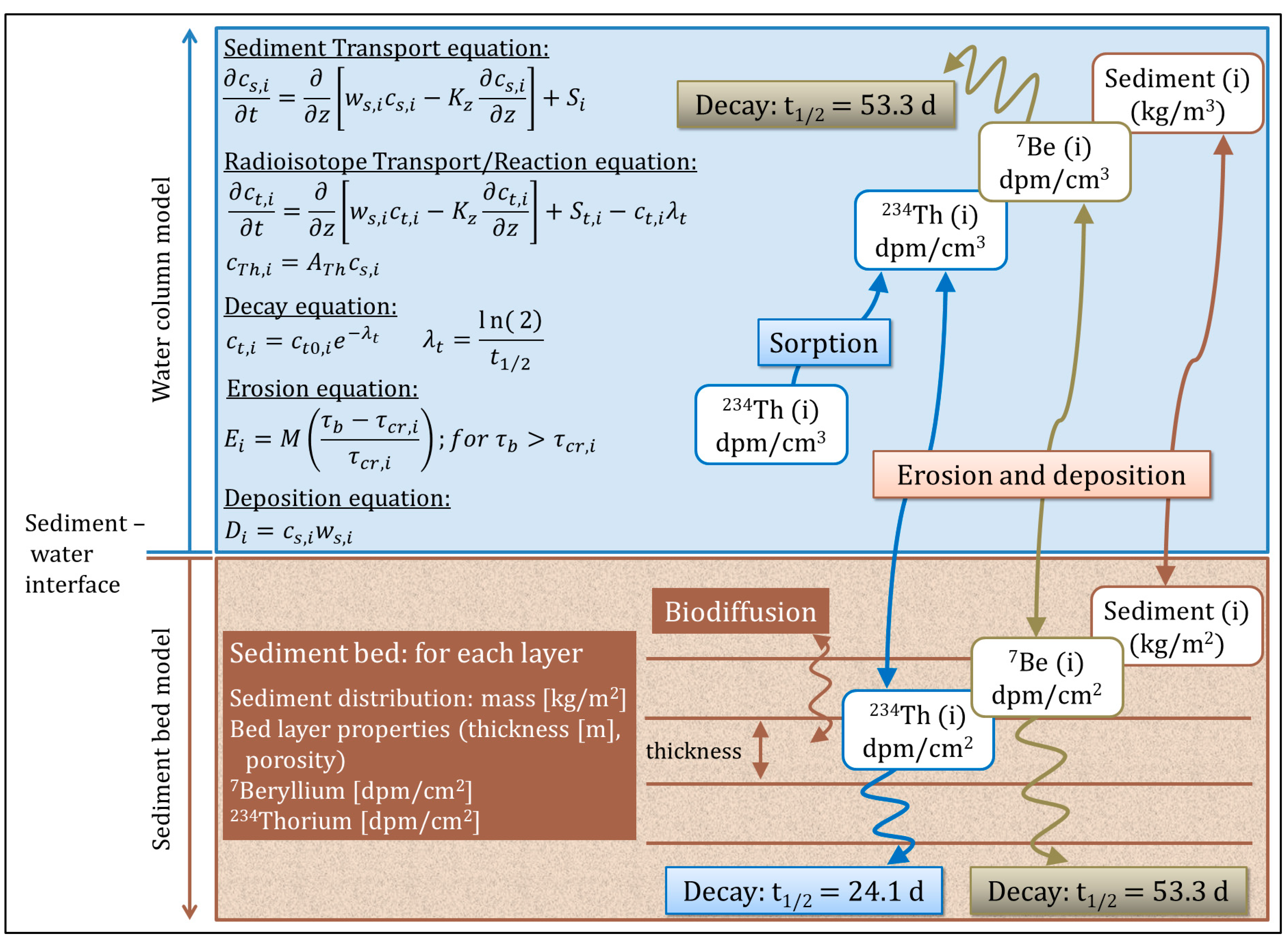
2.1. Adding Reactive Tracers to the CSTMS

The CSTMS [32] operates as a module within the Regional Ocean Modeling System (ROMS; see [35,36]). Within the ocean modeling literature, a tracer refers to a dissolved or particulate scalar quantity that is transported by oceanic flows. Within ROMS, tracers are used to calculate the time-dependent, spatially varying fields of temperature and salinity. ROMS also uses tracers to track concentrations of sediment classes when the sediment module is used [32]; and biochemical constituents (oxygen, phytoplankton, etc.) when the biogeochemical module is used (e.g., [37]). These concentration fields are updated by solving mass balance equations that may include reactive terms for biogeochemical tracers [35,36]. Until recently, however, all implementations of the CSTMS assumed that the sediment classes acted as conservative tracers, so that their water-column concentrations were updated using the transport equation, with erosion and deposition terms for sources and sinks, and no reaction terms.

The sediment model uses tracers to account for a user-specified number of sediment classes (typically size classes) and represents grain size distributions on the seafloor using a user-specified number of sediment bed layers [32,38]. As a model run progresses, bed layer thicknesses and grain size distributions are adjusted to account for erosion and deposition. Additionally, changes to the thickness of the active transport layer, the layer of sediment at the seabed surface available for erosion [39], can modify the surficial bed characteristics. The non-cohesive sediment transport model used here [32] assumes that the active transport layer usually thickens during times of high excess bed shear stress [39], however, the parameter governing the thickness of the active transport layer is poorly constrained. The model also represents bed armoring, which occurs when the more mobile sediment (lower critical shear stresses and settling velocities) has been eroded; leaving the less mobile sediment (higher critical shear stresses and settling velocities) on the bed to form a lag layer that shelters underlying fine sediment from being entrained into the water column (e.g., [40]).

CSTMS applications commonly treat sediment as a conservative tracer, where the only sources and sinks of sediment are at open boundaries and the sediment bed [32]. Sediment resuspension can be stated as a one-dimensional (vertical) mass balance equation:

$$\frac{\partial c_{s,i}}{\partial t}=\frac{\partial }{\partial z}\left(w_{s,i}{c}_{s,i}-K_z\frac{\partial c_{s,i}}{\partial z}\right)+S_i,$$

(1)

where z is the vertical coordinate for height above the seafloor (m, positive upwards); K_z is eddy viscosity (m² s⁻¹); w_s,i is settling velocity (m s⁻¹); c_s,i is the concentration (kg m⁻³); and i designates the sediment class (Figure 1). S_i accounts for external sources or sinks of sediment. Typically, S_i includes fluxes into and out of the bottom cell to account for erosion and deposition. Note that the actual mass balance equation used in ROMS is three-dimensional and discretized for the model coordinate system.

The sediment transport model has recently been enhanced to include reactive tracers whose transport equation includes reaction terms that represent geochemical processes that change (or exchange) quantities in tracer classes [38,41]. Reactive tracer quantities are transported in the water column at the same rate as associated water parcels or sediment with equivalent settling and erosion properties, so they can shadow a water mass or specific sediment class. The sediment bed model was also modified so that reactive tracers could be stored on the sediment bed and undergo exchanges between the water column and seabed. A recent application has used reaction terms to account for both particulate and dissolved geochemically reactive tracers in the seabed and the water column to evaluate the role of resuspension in biogeochemical cycles [42]. Here, we use a similar approach to simulate the transport, deposition, and decay of ⁷Be and ²³⁴Th (Figure 1), as described in the next section.

The one-dimensional (vertical) activity balance equation for a radioisotope is:

$$\frac{\partial c_{t,i}}{\partial t}=\frac{\partial }{\partial z}\left[w_{s,i}{c}_{t,i}-K_z\frac{\partial c_{t,i}}{\partial z}\right]+S_{t,i}-c_{t,i}{\lambda }_t$$

(2)

where c_t,i is suspended tracer concentration (dpm m⁻³), w_s,i is the settling velocity (m s⁻¹), K_z is eddy viscosity (m² s⁻¹), S_t,i is the source/sink term of tracer concentration associated with the sediment class, and λ_t is the tracer decay constant (s⁻¹). The index, i, denotes the sediment class to which this tracer is associated; while the index, t, denotes the reactive tracer. Aside from decay, tracers were assumed to remain associated with the sediment particles, due to the high particle-reactive nature of the tracers, so that desorption was neglected [1,8,9]. This behavior is consistent with previous studies in shelf environments (e.g., [8,43,44]). Because the transport terms (w_s,i, K_z, and S_i) act identically on the tracer class and the associated sediment class, this equation links the tracer activity to the mass concentration of the sediment class.

The boundary conditions for ⁷Be and ²³⁴Th were modified to represent their behavior in coastal environments. In our conceptual model, ⁷Be on river-dominated shelves is associated with fresh sediment delivered by fluvial input and is not significantly influenced by local atmospheric fallout [5]. We represented this by initializing the numerical model with sediment in suspension, notionally delivered by a fluvial source, and assigning this sediment a user-specified ⁷Be activity reflecting the fluvial provenance. As the model ran forward in time, ⁷Be activities behaved according to Equation (2) as ⁷Be-associated sediment settled, deposited, and possibly was resuspended. Th-234 was treated differently. Our conceptual model was that ²³⁴Th is produced in seawater and scavenged by suspended particles [13,14]. We represented this in the numerical model by maintaining at a constant level the activity levels of ²³⁴Th associated with suspended sediment. In our model, c_Th,i = A_Thc_s,i (Figure 1); where A_Th was the assumed activity of suspended sediment (dpm kg⁻¹) and c_s,i was the suspended sediment concentration (kg m⁻³). This approach was equivalent to assuming that the activity of any sediment in suspension immediately equilibrates to the level driven by local seawater activity. This assumes that equilibration in the model occurs over much shorter timescales than the timescales of typical resuspension events and natural removal of ²³⁴Th by sediment, which occurs on the order of days and is dependent on the amount of sediment resuspension [3,19,43]. Once sediment carrying ²³⁴Th enters the sediment bed, activities begin to decay. Through these treatments of the activities of ⁷Be and ²³⁴Th, we can characterize their behavior in a coastal ocean environment with river input and episodic resuspension.

The model tracked sediment mass and reactive tracer activities in terms of concentration (kg m⁻³ and dpm m⁻³) in each grid cell of the water column, and as layer-integrated quantities (km m⁻² and dpm m⁻²) in each sediment bed layer. Erosion and deposition had corresponding influences on the inventory of radioisotope tracers and associated sediment in the water column and sediment bed. During erosion, reactive tracers linked to sediment classes were removed from the surface sediment layer (i.e., the active transport layer) and added to the water column. During deposition, reactive tracers linked to sediment were removed from the water column and returned to the surface sediment bed layer.

When the bed shear stress (τ_b, Pascals, Pa) exceeds the critical shear stress (τ_cr,i, Pa), the model estimates a sediment entrainment rate for each sediment class (i) proportional to the excess shear stress (S = τ_b − τ_cr,i) following the sediment entrainment equation [32]:

$$E_i=M\left(\frac{{\tau }_b-{\tau }_{cr,i}}{{\tau }_{cr,i}}\right),$$

(3)

where E_i is the entrainment rate (kg m⁻² s⁻¹), M is the erosion rate parameter (kg m⁻² s⁻¹), and i denotes the sediment class to which this tracer is associated. The model assumes simultaneous erosion and deposition (Figure 1), with the deposition equal to the settling flux [32]:

$$D_i=c_{s,i}{w}_{s,i},$$

(4)

where D_i is the deposition rate (kg m⁻² s⁻¹) and c_s,i is the suspended-sediment concentration (kg m⁻³) in the bottommost grid cell. Like most implementations of the CSTMS, we assumed that the hydrodynamic properties of sediment (i.e., settling velocity w_s,i and critical shear stress for motion τ_cr,i) remain fixed for each sediment class [32]. This neglects aggregation and disaggregation; settling velocities are fixed for each class because there is no exchange between sediment classes; though these have recently been included in other versions of the CSTMS [38].

We also modified the CSTMS sediment bed model to better represent stratigraphic processes that affect the distribution of radioisotopes in the seabed. The default sediment bed-layering scheme created new bed layers by dividing the bottom layer in half [32]. This can lead to having thick layers near the bed surface, and exponentially thinner layers with depth, so as in our recent work, we modified the scheme to form new layers by peeling off a thin layer from the bottom layer [38,41]. Additionally, we added biodiffusive mixing between bed layers of tracer concentrations and sediment types using a depth-dependent biodiffusion coefficient (see [38]). The biodiffusion coefficient, D_b, generally decreased with depth in the bed until it reached a small value specified in the input files.

Numerical solution of the tracer conservation equations was verified by comparison with the analytical equation for pure decay of initial activity (no erosion, deposition, or mixing) [45,46]. Using typical values for radioisotope activities and decay constants, burial rates, burial depths, and time scales; the model results were found to match analytical solutions [45,46] within 0.1 percent.

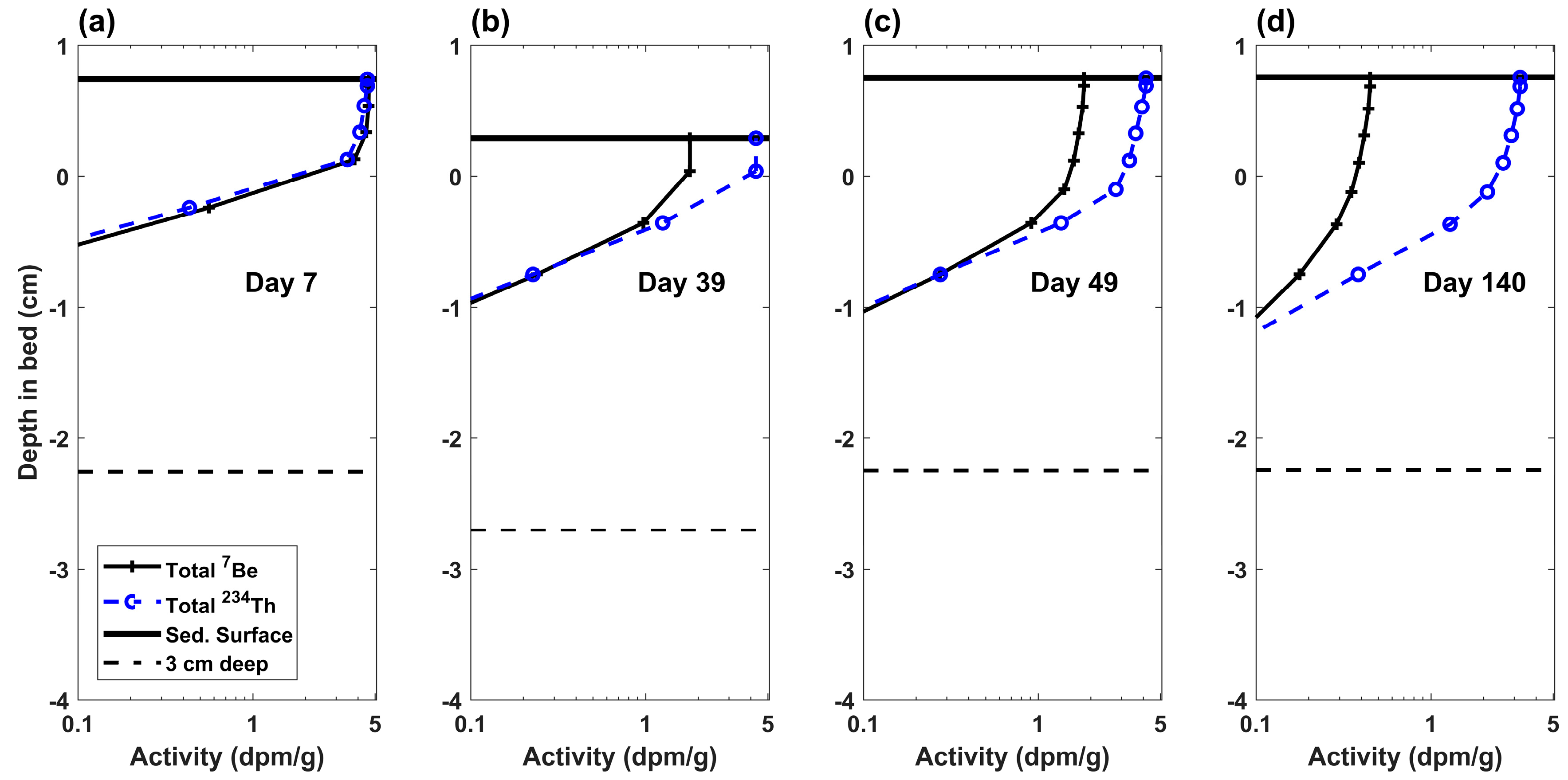
2.2. Idealized Test Case: Model Implementation

This paper presents simulations that explore behavior of the radioisotope tracers within a one-dimensional (vertical) model that represents the water column and underlying sediment bed (Figure 1). Configured similarly to a previously published model [38], our implementation included deposition of a thin fluvial layer and subsequent reworking via idealized storm forcing. Compared to the Standard Model Case, other runs varied parameters to explore sensitivity to the biodiffusion coefficient, resuspension intensity (maximum bed shear stress), and flood deposit thickness. For full details of the model implementation, model code, and input and output files, see the archive [47].

Specifically, the one-dimensional model represented a 20-m deep site using 30 water column layers. Several parameters were based on those used within a three-dimensional ROMS model for the northern Gulf of Mexico [48], including seabed porosity (0.8), and erosion rate parameter (M; 1 × 10⁻⁵ kg m⁻² s⁻¹). The sediment model included three classes: fine (micro-floc), medium (macro-floc), and coarse (sand) with equivalent grain diameters of 15, 63, and 125 micrometers (µm), respectively. These sediment classes assumed a quartz density (2650 kg m⁻³) and had critical shear stresses set to 0.03, 0.08, and 0.1 Pa; and settling velocities of 0.01, 0.1, and 1.0 cm s⁻¹, respectively. The two fine classes represented micro-flocs and macro-flocs, though this version of the model neglected flocculation processes; i.e., the hydrodynamic properties of each class remained fixed and mass was not exchanged between classes. Radioisotopes ⁷Be and ²³⁴Th were linked to the two fine classes and assigned decay constants of λ_Be = 1.51 × 10⁻⁷ s⁻¹ and λ_Th = 3.33 × 10⁻⁷ s⁻¹. The radionuclide adsorption properties were assumed identical for the fine and medium classes.

The upper 10 cm of the sediment bed were represented using 40 sediment layers, most of which were ~5 mm thick. The initial sediment bed grain size distribution was assumed uniform with depth. Unless otherwise specified, biodiffusion occurred throughout the model runs. The biodiffusion coefficient was assumed to vary with depth [38]; for the Standard Case it was set to be 1 cm² yr⁻¹ from the sediment–water interface to a depth of 3 cm, then decreased linearly between 3 to 6 cm below the sediment–water interface. Below 6 cm, it was held constant at 0.02 cm² yr⁻¹.

The water column initially carried suspended concentrations of 0.1 kg m⁻³ for each of the two finest sediment classes, which were tagged with radioisotopes having specific activities of both ⁷Be and ²³⁴Th of 5 dpm g⁻¹, a reasonable value for continental shelves (see Introduction). This material settled out of the water column within the first few days of the model, forming a flood deposit. The initial sediment bed had zero radioisotope inventories. The idealized model was configured to represent a situation where a single flood deposit is reworked by subsequent storm waves. Therefore, ⁷Be was added only at the beginning of the model, and the ⁷Be inventory subsequently decayed. In contrast, the model assumed that ²³⁴Th activities associated with seabed sediment underwent decay, but that ²³⁴Th was replenished upon sediment resuspension. To represent this, the activity of ²³⁴Th on all suspended sediment was instantly reset to 5 dpm g⁻¹.

After the initial suspended sediment settled, the freshly-deposited fluvial layer was subjected to a 125-day idealized stormy period comprised of consecutive two-week intervals that each included a three-day storm and an eleven-day quiescent period (Figure 2a). Sediment was eroded under high bed shear stresses during the storms (2.7 Pa), and then settled and redeposited after bed stresses returned to background levels. The model neglected horizontal flux convergence or divergence, and therefore all sediment eroded during a storm redeposited when conditions subsided. The end of the model included a long quiescent period to evaluate model behavior (Figure 2a–c). Though idealized, the time-series for the wave forcing allows us to examine model behavior for a relatively simple case and has proved useful in past modeling studies [38].

Three sets of experiments used the idealized scenario described above to investigate the sensitivity of seabed radioisotope activities to biodiffusion, flood layer thickness, and resuspension intensity. The Standard Case (Case 1) used intermediate values; while Cases 2–7 each varied one parameter (see

Table 1. Parameters for each model run. Bold print marks the parameters that differ for Cases 2–8.

Case	Db,max (cm2 yr−1)	Bed Stress (Pa)	Flood Layer (cm)	Active Layer (cm)
1	1	2.7	0.75	0.5
2	0	2.7	0.75	0.5
3	25	2.7	0.75	0.5
4	1	0	0.75	0.5
5	1	6	0.75	0.5
6	1	2.7	0.38	0.5
7	1	2.7	1.51	0.5
8	1	2.7	0.75	1.8

). The first set of experiments tested a range of values for biodiffusion coefficients (D_b,max) equal to 0, 1, and 25 cm² yr⁻¹; for Cases 2, 1, and 3, respectively. The second set varied flood input and considered a very thin (0.38 cm, Case 6), thin (0.75 cm, Case 1), and thicker (1.5 cm, Case 7) initial fluvial deposit. The influence of resuspension intensity was considered, both by varying the bed shear stress to include no (0 Pa, Case 4), moderate (2.7 Pa, Case 1), and intense (6.0 Pa, Case 5) resuspension; and by evaluating the sensitivity of radioisotopic profiles to the specification of the active transport layer thickness, i.e., the depth from which sediment can be recruited for resuspension during a model timestep. To prevent the active transport layer from being overly large for Cases 1–7, it was limited to a maximum of 0.5 cm below the sediment bed surface. Case 8 did not limit the active transport layer thickness, but implemented the commonly-used stress-dependent formulation (see [32,39]), via which the active layer thickness reached 1.8 cm.

To analyze the radioisotope behavior, model output was characterized in terms of the calculated penetration depth, radioisotopic inventory, detection timescale, and surface activity; we define those terms here. Surface activity (dpm g⁻¹) represented the average activity in the top 1 cm of the seabed. The radioisotopic inventories (dpm cm⁻²) represented the depth integrals in the bed per cross-sectional area. Penetration depths (cm) of ⁷Be and ²³⁴Th have been used to infer the thicknesses of flood and storm deposits, and for each model run were characterized by the maximum depth below the sediment surface for which the ⁷Be and ²³⁴Th activities exceeded an assumed detection limit of 0.1 dpm g⁻¹. To explore how biodiffusion, resuspension intensity, and flood deposit thickness influenced the likelihood of detection using ⁷Be or ²³⁴Th, we evaluated the detection timescale, calculated as the length of time for which surface activity exceeded 0.1 dpm g⁻¹. The detection timescales of fluvial deposits were calculated as time elapsed since the flood event (i.e., in this case, the first day of the model run) based on detectability of ⁷Be. For storm reworking, the detection timescale of ²³⁴Th was calculated relative to the end of the last resuspension event (Day 125, except for the no resuspension Case 4). We define the thickness of the physically reworked material (cm) as the sum of the thicknesses of the resuspended material and the active transport layer; because this is the thickness of the sediment bed impacted during a storm event by erosion, redeposition, and armoring.

3. Results

The ⁷Be and ²³⁴Th activity profiles changed in response to episodic deposition and resuspension, and persistent biodiffusion and decay (Figure 3). The initial, 0.75 cm-thick, fluvial deposit contained uniformly high ⁷Be and ²³⁴Th activity (Figure 3a). During erosional episodes, activity profiles in the bed changed as sediment that carried radioisotopes was resuspended (Figure 2 and Figure 3b). Upon redeposition, profiles for both radioisotopes showed a surface layer that had uniform activities overlaying sediment whose activities decayed with depth (Figure 3c). Biodiffusion mixed both radioisotopes into the bed throughout the run, which acted to reduce radioisotope activities in the surface layer. As expected, bed inventories of ⁷Be and ²³⁴Th become different during episodes of resuspension, as ²³⁴Th was adsorbed from seawater onto the fine and medium sediment with each storm (Figure 3c,d). In contrast, storm resuspension had no net effect on ⁷Be bed inventory so that, over time, ⁷Be inventories decreased via decay, and surface activities were diluted via biodiffusion. Late in the model, after Day 130, inventories decreased due to the decay of ⁷Be and ²³⁴Th, and surface tracer activities were reduced via biodiffusion (Figure 2d,e).

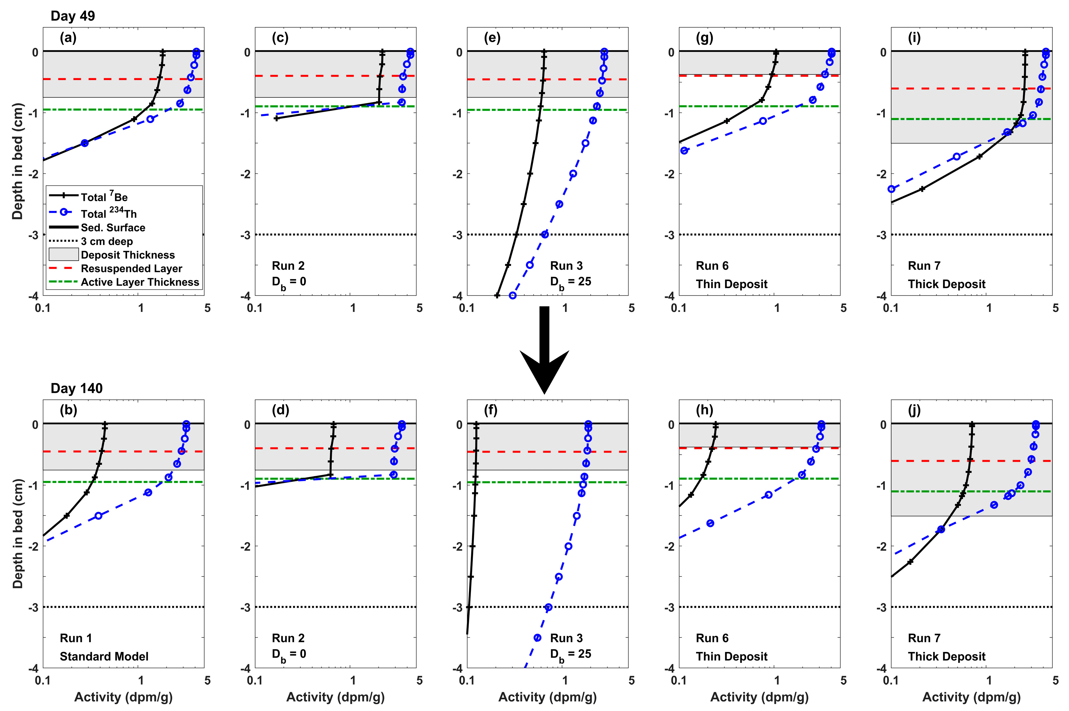
3.1. Sensitivity to Biodiffusivity

Results from model runs that used different biodiffusion coefficients (Cases 1, 2, and 3; Table 1) illustrate the influence of biodiffusion intensity on radioisotope bed profiles. Figure 4a–f shows ⁷Be and ²³⁴Th profiles for these runs after the third and seventh resuspension events (Days 49 and 140, respectively). With increasing biodiffusion intensity, surficial sediments that carry high radioisotope activities were mixed into the seabed at faster rates, increasing the penetration depths for both ²³⁴Th and ⁷Be, and correspondingly decreasing surface activities. However, ²³⁴Th surface activities decreased less than ⁷Be because resuspended sediment adsorbed new ²³⁴Th from seawater, elevating bed inventories of ²³⁴Th as biodiffusion intensity increased. The ²³⁴Th and ⁷Be detection timescales of flood and storm beds decreased with increasing intensity of biodiffusion (

Table 2. Surface activities, bed inventories, penetration depths, and detection timescales after deposition (detection limit = 0.1 dpm g⁻¹) for ⁷Be and ²³⁴Th for all cases. Days 49 and 140 represent times when no sediment was resuspended, but cover a range of time since initial deposition of ⁷Be.

	Day	Standard	Biodiffusion		Resuspension		Thickness		Active
		Case 1	Case 2	Case 3	Case 4	Case 5	Case 6	Case 7	Case 8
7Be Surf. Activity (dpm g−1)	49	1.62	1.97	0.63	1.7	1.56	0.85	2.53	0.79
	140	0.4	0.61	0.12	0.43	0.39	0.21	0.68	0.22
7Be Bed Inventory (dpm cm−2)	49	1.07	1.07	1.07	1.07	1.07	0.53	2.13	1.07
	140	0.33	0.33	0.33	0.33	0.33	0.16	0.66	0.33
7Be Penetration Depth (cm)	49	1.88	1.26	4.94	1.8	1.91	1.55	2.57	3.2
	140	1.88	1.07	3.44	1.77	1.91	1.39	2.56	2.97
7Be TD (months)		8.0	9.6	5.2	8.2	8	6.6	9.4	6.8
234Th Surf. Activity (dpm g−1)	49	3.41	3.51	2.59	0.82	3.56	3.04	3.85	3.7
	140	2.72	2.87	1.82	0.05	2.86	2.52	3	2.96
234Th Bed Inventory (dpm cm−2)	49	2.07	1.87	3.19	0.51	2.27	1.8	2.75	4.58
	140	1.75	1.52	2.74	0.04	1.95	1.58	2.1	3.73
234Th Penetration Depth (cm)	49	1.86	1.09	5.03	1.48	1.93	1.69	2.25	3.42
	140	1.97	1.09	5.7	0	2.11	1.96	2.21	3.49
234Th TD (months)		4.2	4.6	3.2	4.1	4.3	4.1	4.3	4.4

). As D_b,max increased, each radioisotope was mixed more rapidly into the bed, diluting surface activities by vertical mixing, so that surface activities fell below the detection limit more quickly.

3.2. Sensitivity to Fluvial Deposit Thickness

Cases 6 and 7 had initial fluvial deposit thicknesses of 0.38 and 1.5 cm, one-half and double the deposit thickness of Case 1, respectively. Because the fluvial deposit provided the initial source of radioisotopes to the seabed, the deposit thickness directly influenced penetration depth and bed inventory for both radioisotopes early in the model run (Figure 4a,g,i; Table 2). Physical mixing was especially important for Case 6, for which the thickness of the resuspended layer exceeded that of the initial fluvial deposit.

The ⁷Be surface activity remained higher over time for the thicker deposits than for the thinner deposit, but the differences did not scale linearly with deposit thickness due to physical and biological mixing (Figure 4; Table 2). Doubling the fluvial deposit thickness increased the ⁷Be surface activity by 56% and the ⁷Be penetration depth by 37% on day 49 of the model runs (Table 2). The initial fluvial thickness played an even smaller role in the detection timescale, with thicker deposits remaining detectable for only slightly longer than calculated for the thinner deposits; doubling the flood thickness increased the detection timescale for ⁷Be by roughly 18% (Table 2).

The relative thicknesses of the physically reworked layer compared with the initial flood deposit affected the response of the ²³⁴Th activities. Cases 1 and 6 had similar ²³⁴Th penetration depths (Figure 4a,b,g,h; Table 2) because they were set by the thickness of the physically reworked layers. The fact that the initial fluvial deposit thickness for Case 7 exceeded that of the resuspended layer directly affected the penetration depth (Figure 4a,i; Table 2). There was feedback between fluvial deposit thickness and mass of sediment resuspended, because the fluvial layer only contained fine and medium sediment. A thicker fluvial layer therefore supplied more fine and medium sediment near the surface, allowing more mobile sediment to be eroded and become tagged with fresh ²³⁴Th in the water column. This increased the ²³⁴Th inventories and penetration depths after resuspension events (Table 2).

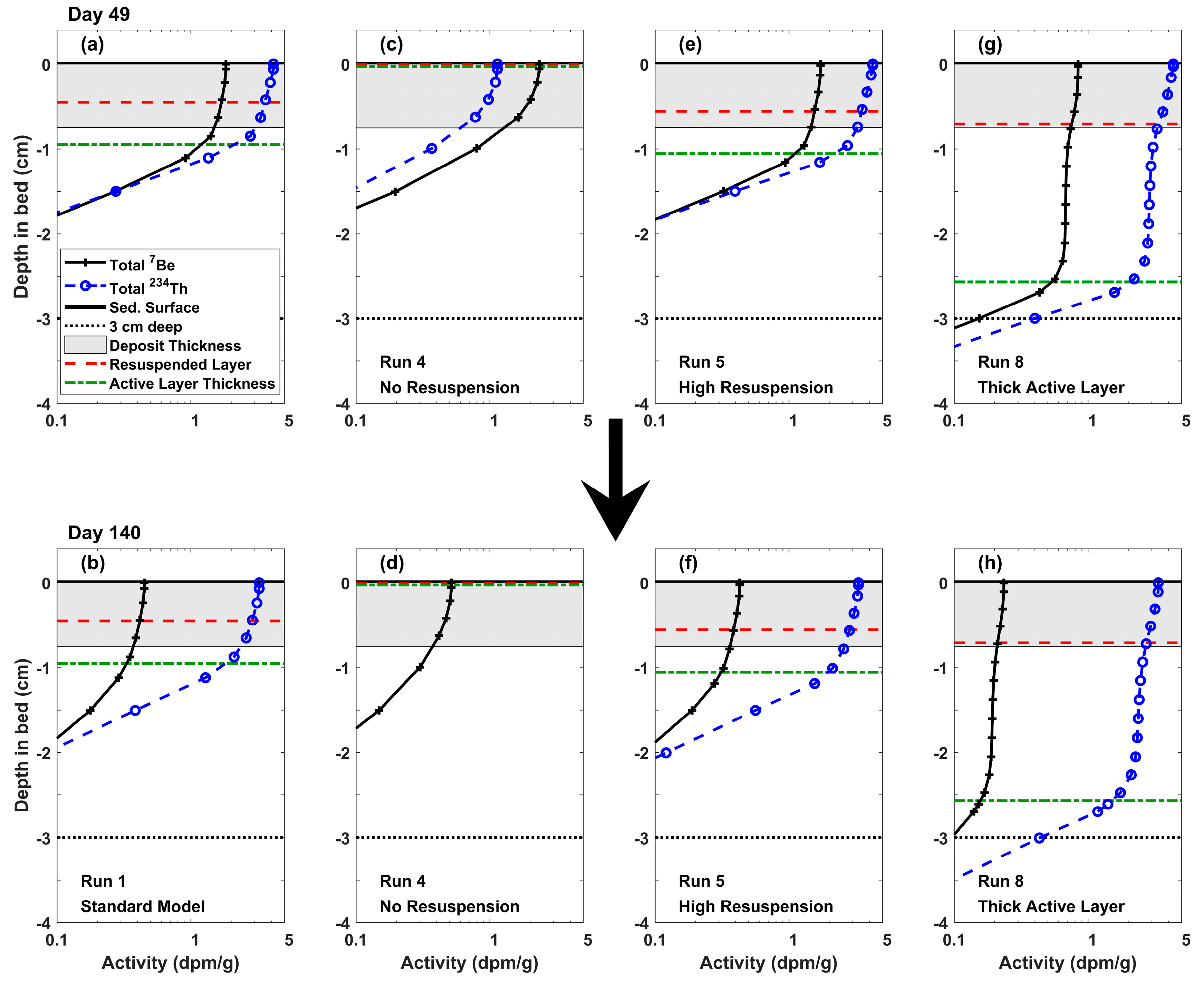
3.3. Sensitivity to Resuspension Intensity

Cases 4 and 5 explored how the seabed profiles of ⁷Be and ²³⁴Th responded to changes in resuspension intensity by varying the magnitude of the maximum bed shear stress, τ_b. The cases featuring zero (Case 4), medium (Case 1), and high resuspension intensity (Case 5) yielded erosion depths of 0, 0.46, and 0.56 cm, respectively (Figure 5). For the cases that included resuspension, the thickness of the fluvial deposit (0.75 cm) exceeded the peak erosion depths. Bed inventories of ²³⁴Th increased with resuspension intensity; energetic events suspended more sediment which then scavenged ²³⁴Th from the water column (Table 2). The case with no resuspension therefore had much lower ²³⁴Th surface activity and bed inventory than the other cases (Figure 5c,d). In contrast, resuspension did not affect ⁷Be bed inventories, as the model assumed that ⁷Be was only supplied in the initial flood deposit. Via physical mixing, erosion and redeposition cycles increased penetration depths for both radioisotopes. During periods of erosion, the active transport layers shifted deeper into the seabed, mixing radioisotope-tagged surficial sediments with underlying lower-activity sediment. This decreased surface activities and detection time-scales with increasing resuspension intensity for ⁷Be, because it was not replenished during storms.

Case 8 evaluated the role of the active layer thickness on resuspension intensity and its impact on modeled radioisotope profiles. While other cases limited the active transport layer thickness to a maximum of 0.5 cm, Case 8 used a widely accepted formulation (i.e., [39]) for it that reached 1.8 cm during the storm. Therefore, though bed stresses were identical, the amount of suspended sediment and the eroded depth was almost doubled in Case 8 compared to Case 1. The active transport layer thickness also greatly influenced the modeled radioisotope signatures (Figure 5a,b,g,h). While total ⁷Be bed inventory was insensitive to the active transport layer thickness, the increased erosion and concurrent mixing of the surficial few centimeters of the bed effectively diluted the surface activity for ⁷Be and increased the penetration depth (Figure 5a,b,g,h). In contrast, the surface activity of ²³⁴Th was insensitive to the increased active transport layer thickness, (Table 2, Figure 5a,b,g,h), but the resultant higher resuspension depths nearly doubled the ²³⁴Th inventory and the penetration depths for Case 8 relative to Case 1 (Table 2, Figure 5a,b,g,h).

4. Discussion

4.1. Synthesis of Sensitivity Tests

The results summarized in Table 2 demonstrate that variable bioturbation rates, resuspension intensity, initial flood deposit thickness, and active layer thickness affected modeled radioisotope profiles, inventories, penetration depths, and detection time scales to varying degrees. The biodiffusion sensitivity tests (Cases 2 and 3) generated results that deviated most from Case 1. Note that these biodiffusion rates spanned a larger range than considered in the other sensitivity trials, but this reflects the significant uncertainty in characterizing biodiffusion coefficients (see [46]). In Case 3, enhanced bioturbation increased the ²³⁴Th and ⁷Be penetration depths, reduced surface activities, and caused the shortest detection timescales for any of the model runs (Table 2, Figure 4 and Figure 5). Case 2 neglected biodiffusion and produced the thinnest penetration depth and longest detection time scale of the cases considered (Table 2). Varying the initial fluvial layer thickness appreciably affected the ⁷Be results, especially ⁷Be bed inventory, more so than ²³⁴Th. Results from the cases that investigated resuspension intensity and active layer thickness suggested that increasing resuspension, in the presence of bioturbation, worked to dissipate the terrestrial ⁷Be signal, while enhancing the oceanic ²³⁴Th signal.

The reactive tracer model responded reasonably to a range of dissipative and intensifying conditions for two radioisotopes that are indicative of terrestrial and oceanic sources. Analysis of the idealized test case results produced radioisotope profiles and metrics similar to those observed on continental shelf environments (e.g., [5,9,17]), and consistent with patterns noted in field observations. For example, bioturbative processes are known to mix radioisotopes into the seabed, increasing penetration depths and reducing detection time scales [16,17,23,25]. Similar to the results that varied fluvial layer thickness (Cases 6 and 7; Figure 4; Table 2), bed inventories of ²³⁴Th and ⁷Be have been observed to correlate positively with initial flood layer thickness [5]. Model experiments also provided scenarios wherein shorter-lived ²³⁴Th was observed at greater depth than the longer-lived ⁷Be (Cases 1, 3, 6, 8) as observed in the Adriatic Sea [9].

4.2. Limitations of Model as Implemented Here

This model marks a first step in integrating sediment transport process models [32] with the radioisotopic tracers that have been increasingly used as indicators of sediment transport processes (e.g., [3,5,6,7,9,13]). This section reviews some of the assumptions that were made in developing this model and discusses their implications.

The model discussed herein used a relatively simple approach to represent behavior of radioisotopes, but integrated them into an established sediment transport model. In particular, the model employed a simple conceptual model for the sources of the radioisotopes, and for their interactions with sediment that would be appropriate for river-dominated areas where these radioisotopes have been used to infer source and transport processes. To represent an initial flood source for sediment, the only source of ⁷Be was assumed to be sediment suspended at the start of the model run, which had a prescribed activity of associated ⁷Be. While it is known that activities of fluvially discharged ⁷Be vary in time [9], our idealized scenario represented only an initial flood pulse so that temporal variation in ⁷Be was not an issue for the runs presented. Additionally, our conceptual model neglected other sources of ⁷Be; for example, direct precipitation has been noted as a source of ⁷Be on non-river influenced continental shelves [49]. Similarly, the conceptual model simplified the processes that influence ²³⁴Th activities in coastal environments. The model also assumed that all suspended sediment carried a constant, pre-set activity of ²³⁴Th. This was equivalent to assuming that sorption of ²³⁴Th to sediment grains occurred instantaneously upon suspension in the model water column, and that there was no variation in background ²³⁴Th concentrations. In actuality, the association of ²³⁴Th with suspended sediment grains may take days to equilibrate, dependent on suspended sediment concentrations [3,19,43], and ²³⁴Th concentrations are known to vary with salinity within estuaries and on river-influenced shelves [1]. Additionally, the model assumed that the activities of the radioisotopes on the muddy sediment did not vary with grain size or water column properties.

The sediment transport model also included some simplifications. For example, the resuspension of muddy sediment is subjected to cohesive processes such as bed consolidation and flocculation. The version of the CSTMS used here [32] neglected these processes, so that the sediment classes had pre-set, constant values to represent erodibility and settling velocity. For application to reworking of muddy flood deposits, future studies might consider using the radioisotopic reactive tracer module presented here with the version of the CSTMS that also accounts for flocculation and bed consolidation [38].

Bedload was not directly represented in our model, though the CSTMS provides bedload formulations that can be applied to the upper-most sediment bed layer, i.e., the active transport layer [32]. We did not use the bedload transport formulations, however. Because our idealized one-dimensional (vertical) model assumes uniform horizontal sediment fluxes, there would be no net erosion or deposition from bedload. One conceptualization of the active transport layer, however, is as a bedload layer from which sediment can be suspended [40]. As bedload intensifies, the active layer thickens, which in our model acted to mix and dilute the radioisotope tracer concentrations in the upper sediment bed. The sensitivity of surface activity and penetration depth to the formulation of the active transport layer (Cases 1 and 8) illustrates this.

4.3. Future Applications

As discussed in the previous section, our idealized model used a relatively simple representation of radioisotopes and neglected some sediment transport processes. Though this model did not represent the full complexities of actual radioisotope source terms, or particle–radioisotope interactions, the model itself could provide a venue for future studies that consider the impact of these complexities on sediment bed geochronological tracer profiles. Additionally, by developing our coupled reactive tracer–sediment transport model within a community modeling framework, this paves the way for future studies to consider the potential impacts of other sediment transport processes or radioisotopic chemistry on the geochronological record.

In addition to idealized studies such as reported here, the geochronological model should provide useful insight if applied to realistic field settings. For example, we have used a similar one-dimensional (vertical) version of the model to represent a site offshore of the Mississippi subaqueous delta [50]. This model was implemented to replicate observed radioisotopic profiles [6]. The model-produced radioisotopic profiles were then used within various analytical models from the literature to derive deposition rate, etc., from the simulated profiles; which were then compared to the actual model deposition rates. Results showed that the analytical model estimates can be unreliable if assumptions regarding the biodiffusion rate and radioisotope activity of freshly deposited sediment are incorrect [50].

It would be useful to add the capability of our sediment transport geochronological model to a full three-dimensional model, such as that developed for the Waipaoa River Shelf, NZ [51], or a northern Gulf of Mexico continental shelf model [48,52]. Both of these efforts attempted to use radioisotopic data for comparison to model estimates of sediment deposition; but this exercise presented challenges that may be abated by direct inclusion of the radioisotopes within the transport equations. Accounting for geochronology within realistic domain models could facilitate model validation by enabling direct comparison between the modeled and measured quantities, i.e., profiles of ²³⁴Th and ⁷Be. Within a joint field and modeling study, this capability could enable careful model–data comparisons that could yield insight into the specification of some model parameters that have been difficult to constrain, such as the active transport layer thickness.

5. Conclusions

A sediment transport model has been modified to account for reactive terms and represent transformations of particulate tracers in the water column and seabed. The model was applied to calculate sediment bed profiles of short half-life radioisotopes ⁷Be and ²³⁴Th that have been used to interpret deposits of river derived sediment and marine sediment resuspension, respectively. Examples were provided in an idealized one-dimensional (vertical) model that represented sediment suspension and the seabed, and that evaluated the response of radioisotope profiles to variations in riverine sediment input, storm intensity, and biodiffusive mixing coefficient. Radioisotopic values such as surface activity, inventory, and penetration depth were analyzed from model results and compared to the sediment input and reworking represented in the model. The intensity of biodiffusion affected the persistence of detectable fluvial event beds. Using a biodiffusion coefficient of 25 cm² yr⁻¹, the fluvial event bed would be obscured within days or weeks. Both resuspension and biodiffusion increased the seabed inventory of ²³⁴Th. Biodiffusion diluted the surface layer by mixing sediment enriched with ²³⁴Th (and ⁷Be) with underlying material. When surficial sediment underwent cycles of resuspension and redeposition, however, it became enriched in ²³⁴Th and thereby increased the total bed inventory upon redeposition.

References

1. Waples, J.T.; Benitez-Nelson, C.; Savoye, N.; Rutgers van der Loeff, M.; Baskaran, M.; Gustafsson, O. An introduction to the application and future use of 234Th in aquatic systems. Mar. Chem. 2006, 100, 166–189. [Google Scholar] [CrossRef]
2. Dibb, J.E.; Rice, D.L. Geochemistry of beryllium-7 in Chesapeake Bay. Estuar. Coast. Shelf Sci. 1989, 28, 379–394. [Google Scholar] [CrossRef]
3. Feng, H.; Cochran, J.K.; Hirschberg, D.J. 234Th and 7Be as tracers for the transport and dynamics of suspended particles in a partially mixed estuary. Geochim. Cosmochim. Acta 1999, 63, 2487–2505. [Google Scholar] [CrossRef]
4. Kniskern, T.A.; Kuehl, S.A. Spatial and temporal variability of seabed disturbance in the York River subestuary. Estuar. Coast. Shelf Sci. 2003, 58, 37–55. [Google Scholar] [CrossRef]
5. Sommerfield, C.K.; Nittrouer, C.A.; Alexander, C.R. 7Be as a tracer of flood sedimentation on the northern California continental margin. Cont. Shelf Res. 1999, 19, 225–361. [Google Scholar] [CrossRef]
6. Corbett, D.R.; McKee, B.A.; Duncan, D. An evaluation of mobile mud dynamics in the Mississippi River deltaic region. Mar. Geol. 2004, 209, 91–112. [Google Scholar] [CrossRef]
7. Kniskern, T.A.; Mitra, S.; Orpin, A.R.; Harris, C.K.; Walsh, J.P.; Corbett, D.R. Characterization of a flood-associated deposit on the Waipaoa River shelf using radioisotopes and terrigenous organic matter abundance and composition. Cont. Shelf Res. 2014, 86, 66–84. [Google Scholar] [CrossRef]
8. Baskaran, M.; Santschi, P.H. The role of particles and colloids in the transport of radionuclides in coastal environments of Texas. Mar. Chem. 1993, 43, 95–114. [Google Scholar] [CrossRef]
9. Palinkas, C.M.; Nittrouer, C.A.; Wheatcroft, R.A.; Langone, L. The use of 7Be to identify event and seasonal sedimentation near the Po River delta, Adriatic Sea. Mar. Geol. 2005, 222–223, 95–112. [Google Scholar] [CrossRef]
10. Mullenbach, B.L.; Nittrouer, C.A. Rapid deposition of fluvial sediment in the Eel Canyon, northern California. Cont. Shelf Res. 2000, 20, 2191–2212. [Google Scholar] [CrossRef]
11. Corbett, D.R.; Dail, M.; McKee, B.A. High-frequency time-series of the dynamic sedimentation processes on the western shelf of the Mississippi River Delta. Cont. Shelf Res. 2007, 27, 1600–1615. [Google Scholar] [CrossRef]
12. Boudreau, B.P. Is burial velocity a master parameter for bioturbation? Geochim. Cosmochim. Acta 1994, 58, 1243–1249. [Google Scholar] [CrossRef]
13. McKee, B.A.; DeMaster, D.J.; Nittrouer, C.A. The use of 234Th/238U disequilibrium to examine the fate of particle-reactive species on the Yangtze continental shelf. Earth Planet. Sci. Lett. 1984, 68, 431–442. [Google Scholar] [CrossRef]
14. Smoak, J.M.; DeMaster, D.J.; Kuehl, S.A.; Pope, R.H.; McKee, B.A. The behavior of particle-reactive tracers in a high turbidity environment: 234Th and 210Pb on the Amazon continental shelf. Geochim. Cosmochim. Acta 1996, 60, 2123–2137. [Google Scholar] [CrossRef]
15. Aller, R.C.; Benninger, L.K.; Cochran, J.K. Tracking particle-associated processes in nearshore environments by use of 234Th/238U disequilibrium. Earth Planet. Sci. Lett. 1980, 47, 161–175. [Google Scholar] [CrossRef]
16. Wheatcroft, R.A. Time-series measurements of macrobenthos abundance and sediment bioturbation intensity on a flood-dominated shelf. Prog. Oceanogr. 2006, 71, 88–122. [Google Scholar] [CrossRef]
17. Wheatcroft, R.A.; Drake, D.E. Post-depositional alteration and preservation of sedimentary event layers on continental margins, I. The role of episodic sedimentation. Mar. Geol. 2003, 199, 123–137. [Google Scholar] [CrossRef]
18. Dibb, J.E. Atmospheric deposition of beryllium-7 in the Chesapeake Bay region. J. Geophys. Res. 1989, 94, 2261–2265. [Google Scholar] [CrossRef]
19. Aller, R.C.; Cochran, J.K. 234Th/238U Disequilibrium in near-shore sediment: Particle reworking and diagenetic time scales. Earth Planet. Sci. Lett. 1976, 29, 37–50. [Google Scholar] [CrossRef]
20. McKee, B.A.; Nittrouer, C.A.; DeMaster, D.J. Concepts of sediment deposition and accumulation applied to the continental shelf near the mouth of the Yangtze River. Geology 1983, 11, 631–633. [Google Scholar] [CrossRef]
21. Wheatcroft, R.A. Preservation potential of sedimentary event layers. Geology 1990, 18, 843–845. [Google Scholar] [CrossRef]
22. Wheatcroft, R.A.; Wiberg, P.L.; Alexander, C.R.; Bentley, S.J.; Drake, D.E.; Harris, C.K.; Ogston, A.S. Post-depositional alteration and preservation of sedimentary strata. In Continental-Margin Sedimentation: From Sediment Transport to Sequence Stratigraphy; International Association of Sedimentologists Special Publication no. 37; Nittrouer, C.A., Austin, J.A., Field, M.E., Kravitz, J.H., Syvitski, J.P.M., Wiberg, P.L., Eds.; Blackwell Publishing: Malden, MA, USA, 2007; pp. 101–155. ISBN 9781405169349. [Google Scholar]
23. Nittrouer, C.A.; DeMaster, D.J.; McKee, B.A.; Cutshall, N.H.; Larson, I.L. The effect of sediment mixing on Pb-210 accumulation rates for the Washington continental shelf. Mar. Geol. 1984, 54, 201–221. [Google Scholar] [CrossRef]
24. Bentley, S.J.; Sheremet, A.; Jaeger, J.M. Event sedimentation, bioturbation, and preserved sedimentary fabric: Field and model comparisons in three contrasting marine settings. Cont. Shelf Res. 2006, 26, 2108–2124. [Google Scholar] [CrossRef]
25. Nittrouer, C.A.; Sternberg, R.W. The formation of sedimentary strata in an allochthonous shelf environment: The Washington continental shelf. Mar. Geol. 1981, 42, 201–232. [Google Scholar] [CrossRef]
26. Sadler, P.M. The influence of hiatuses on sediment accumulation rates. GeoRes. Forum 1999, 5, 15–40. [Google Scholar]
27. Bentley, S.J.; Sheremet, A. New model for the emplacement, bioturbation and preservation of fine-scaled sedimentary strata. Geology 2003, 31, 725–728. [Google Scholar] [CrossRef]
28. Ma, Y.; Friedrichs, C.T.; Harris, C.K.; Wright, L.D. Deposition by seasonal wave- and current-supported sediment gravity flows interacting with spatially varying bathymetry: Waiapu shelf, New Zealand. Mar. Geol. 2010, 275, 199–211. [Google Scholar] [CrossRef]
29. Kniskern, T.A.; Kuehl, S.A.; Harris, C.K.; Carter, L. Sediment accumulation patterns and fine-scale strata formation on the Waiapu River shelf, New Zealand. Mar. Geol. 2010, 270, 188–201. [Google Scholar] [CrossRef]
30. Lesser, G.R.; Roelvink, J.A.; van Kester, J.A.T.M.; Stelling, G.S. Development and validation of a three-dimensional morphological model. Coast. Eng. 2004, 51, 883–915. [Google Scholar] [CrossRef]
31. Neumeier, U.; Ferrarin, C.; Amos, C.L.; Umgiesser, G.; Li, M.Z. Sedtrans05: An improved sediment-transport model for continental shelves and coastal waters with a new algorithm for cohesive sediments. Comput. Geosci. 2008, 34, 1223–1242. [Google Scholar] [CrossRef]
32. Warner, J.C.; Sherwood, C.R.; Signell, R.P.; Harris, C.K.; Arango, H.G. Development of a three-dimensional, regional, coupled wave, current, and sediment-transport model. Comput. Geosci. 2008, 34, 1284–1306. [Google Scholar] [CrossRef]
33. Moriarty, J.M.; Harris, C.K.; Hadfield, M.G. A hydrodynamic and sediment transport model for the Waipaoa Shelf, New Zealand: Sensitivity of fluxes to spatially-varying erodibility and model nesting. J. Mar. Sci. Eng. 2014, 2, 336–369. [Google Scholar] [CrossRef]
34. Palinkas, C.M.; Halka, J.P.; Li, M.; Sanford, L.P.; Cheng, P. Sediment deposition from tropical storms in the upper Chesapeake Bay: Field observations and model simulations. Cont. Shelf Res. 2014, 86, 6–16. [Google Scholar] [CrossRef]
35. Haidvogel, D.B.; Arango, H.; Budgell, W.P.; Cornuelle, B.D.; Curchitser, E.; Di Lorenzo, E.; Fennel, K.; Geyer, W.R.; Hermann, A.J.; Lanerolle, L.; et al. Ocean forecasting in terrain-following coordinates: Formulation and skill assessment of the regional ocean modeling system. J. Comput. Phys. 2008, 227, 3595–3624. [Google Scholar] [CrossRef]
36. Shchepetkin, A.F.; McWilliams, J.C. The regional oceanic modeling system (ROMS): A split-explicit, free-surface, topography-following-coordinate oceanic model. Ocean Model. 2005, 9, 347–404. [Google Scholar] [CrossRef]
37. Fennel, K.; Wilkin, J.; Previdi, M.; Najjar, R. Denitrification effects on air-sea CO2 flux in the coastal ocean: Simulations for the northwest North Atlantic. Geophys. Res. Lett. 2008, 35, L24608. [Google Scholar] [CrossRef]
38. Sherwood, C.R.; Aretxabaleta, A.L.; Harris, C.K.; Rinehimer, J.P.; Verney, R.; Ferré, B. Cohesive and mixed sediment in the Regional Ocean Modeling System (ROMS v3.6) implemented in the Coupled Ocean–Atmosphere–Wave–Sediment Transport Modeling System (COAWST r1234). Geosci. Model Dev. 2018, 11, 1849–1871. [Google Scholar] [CrossRef] [Green Version]
39. Harris, C.K.; Wiberg, P.L. Approaches to quantifying long-term continental shelf sediment transport with an example from the northern California STRESS mid-shelf site. Cont. Shelf Res. 1997, 17, 1389–1418. [Google Scholar] [CrossRef]
40. Wiberg, P.L.; Drake, D.E.; Cacchione, D.A. Sediment resuspension and bed armoring during high bottom stress events on the northern California inner continental shelf: Measurements and predictions. Cont. Shelf Res. 1994, 14, 1191–1219. [Google Scholar] [CrossRef]
41. Moriarty, J.M.; Harris, C.K.; Fennel, K.; Friedrichs, M.A.; Xu, K.; Rabouille, C. The roles of resuspension, diffusion and biogeochemical processes on oxygen dynamics offshore of the Rhône River, France: A numerical modeling study. Biogeosciences 2017, 14, 1919–1946. [Google Scholar] [CrossRef]
42. Moriarty, J.M.; Harris, C.K.; Friedrichs, M.A.M.; Fennel, K.; Xu, K. Impact of seabed resuspension on oxygen and nitrogen dynamics in the northern Gulf of Mexico: A numerical modeling study. J. Geophys. Res. Oceans 2018, 123, 1–27. [Google Scholar] [CrossRef]
43. Santschi, P.H.; Li, Y.-H.; Bell, J.J. Natural radionuclides in Narragansett Bay. Earth Planet. Sci. Lett. 1979, 47, 201–213. [Google Scholar] [CrossRef]
44. Baskaran, M.; Ravichandran, M.; Bianchi, T.S. Cycling of 7Be and 210Pb in a high DOC, shallow, turbid estuary of south-east Texas. Estuar. Coast. Shelf Sci. 1997, 45, 165–176. [Google Scholar] [CrossRef]
45. Carslaw, H.S.; Jaeger, J.C. Conduction of Heat in Solids; Clarendon Press: Oxford, UK, 1959; ISBN 9780198533689. [Google Scholar]
46. Boudreau, B.P. Diagenetic Models and Their Interpretation; Springer: Berlin, Germany, 1997; ISBN 9783642643996. [Google Scholar]
47. Birchler, J.J.; Harris, C.K.; Kniskern, T.A. A Model Archive for Sediment Transport Model Including Short-Lived Radioisotopes: Model Description and Idealized Test Cases; Virginia Institute of Marine Science, College of William and Mary: Gloucester Point, VA, USA, 2018. [Google Scholar]
48. Xu, K.; Harris, C.K.; Hetland, R.D.; Kaihatu, J.M. Dispersal of Mississippi and Atchafalaya sediment on the Texas-Louisiana shelf: Model estimates for the year 1993. Cont. Shelf Res. 2011, 31, 1558–1575. [Google Scholar] [CrossRef]
49. Benitez-Nelson, C.R.; Buesseler, K.O.; Crossin, G. Upper ocean carbon export, horizontal transport, and vertical eddy diffusivity in the southwestern Gulf of Maine. Cont. Shelf Res. 2000, 20, 707–736. [Google Scholar] [CrossRef]
50. Birchler, J.J.; Harris, C.K.; Kniskern, T.A.; Sherwood, C.R. Numerical model of geochronological tracers for deposition and reworking applied to the Mississippi subaqueous delta. J. Coast. Res. Spec. Issue 85 Proc. 5th Int. Coast. Symp. 2018, 456–460. [Google Scholar] [CrossRef]
51. Moriarty, J.M.; Harris, C.K.; Hadfield, M.G. Event-to-seasonal sediment dispersal on the Waipaoa River Shelf, New Zealand: A numerical modeling study. Cont. Shelf Res. 2015, 110, 108–123. [Google Scholar] [CrossRef]
52. Xu, K.; Mickey, R.C.; Chen, Q.J.; Harris, C.K.; Hetland, R.; Hu, K.; Wang, J. Shelf sediment transport during Hurricanes Katrina and Rita. Comput. Geosci. 2016, 90, 24–39. [Google Scholar] [CrossRef]
Figure 1. Schematics of the sediment transport and geochronology model. Water column layers (blue) overlie seabed layers (brown) of variable thickness. Shaded boxes indicate processes; white boxes indicate state variables (tracers).
Jmse 06 00144 g001
Figure 2. Time series for the Standard Case (Case 1) of (a) bed stress, (b) depth-averaged suspended sediment concentrations (see legend), (c) bed thickness relative to initial, (d) radioisotope bed inventories, and (e) radioisotope surface activities. Shows first 200 days of 365-day run. Conditions remained quiescent after Day 130.
Jmse 06 00144 g002
Figure 3. Vertical profiles of seabed radioisotope activities at four instances for Case 1. (a) Day 7 after initial deposition, (b) Day 39 at peak of a resuspension event, (c) Day 49 after redeposition, and (d) Day 140 during the extended quiescent period. Solid black lines represent bed surface and thick dashed lines represent three centimeters deep in the bed. The bed height prior to initial deposition was defined as zbed = 0.
Jmse 06 00144 g003
Figure 4. Radioisotope profiles calculated that (a,b) used Db,max = 1 cm2 yr−1 and had a flood deposit 0.75 cm thick (Case 1), (c,d) neglected biodiffusion (Case 2), (e,f) used Db,max = 25 cm2 yr−1 (Case 3), (g,h) had a flood deposit 0.38 cm thick (Case 4), and (i,j) had a flood deposit 1.51 cm thick (Case 5). Top row shows results on Day 49 while bottom row shows Day 140. Horizontal lines are as described in Figure 3. The gray box represents the extent of the initial flood deposit, red line denotes depth of resuspended layer, green line denotes the maximum penetration of the active layer when sediment was resuspended. The bed height after initial deposition is defined as zbed = 0.
Jmse 06 00144 g004
Figure 5. Radioisotope profiles that had (a,b) resuspension depth of 0.46 cm (Case 1), (c,d) no resuspension (Case 4), (e,f) resuspension depth of 0.56 cm (Case 6), and (g,h) a thick active layer (Case 8). Top row shows results on day 49; while bottom row shows day 140. Horizontal lines as described in Figure 3. Gray boxes represent the initial extents of the flood deposit, red lines denote depth of resuspended layer, green lines denote depth of maximum active layers. The bed height after deposition was defined as zbed = 0. Note that day 140 for Run 4 (d) has zero 234Th, which decayed below the detection limit by this time.
Jmse 06 00144 g005