Autonomous Minimum Safe Distance Maintenance from Submersed Obstacles in Ocean Currents


Abstract
Featured Application
Abstract
1. Introduction
2. Materials and Methods
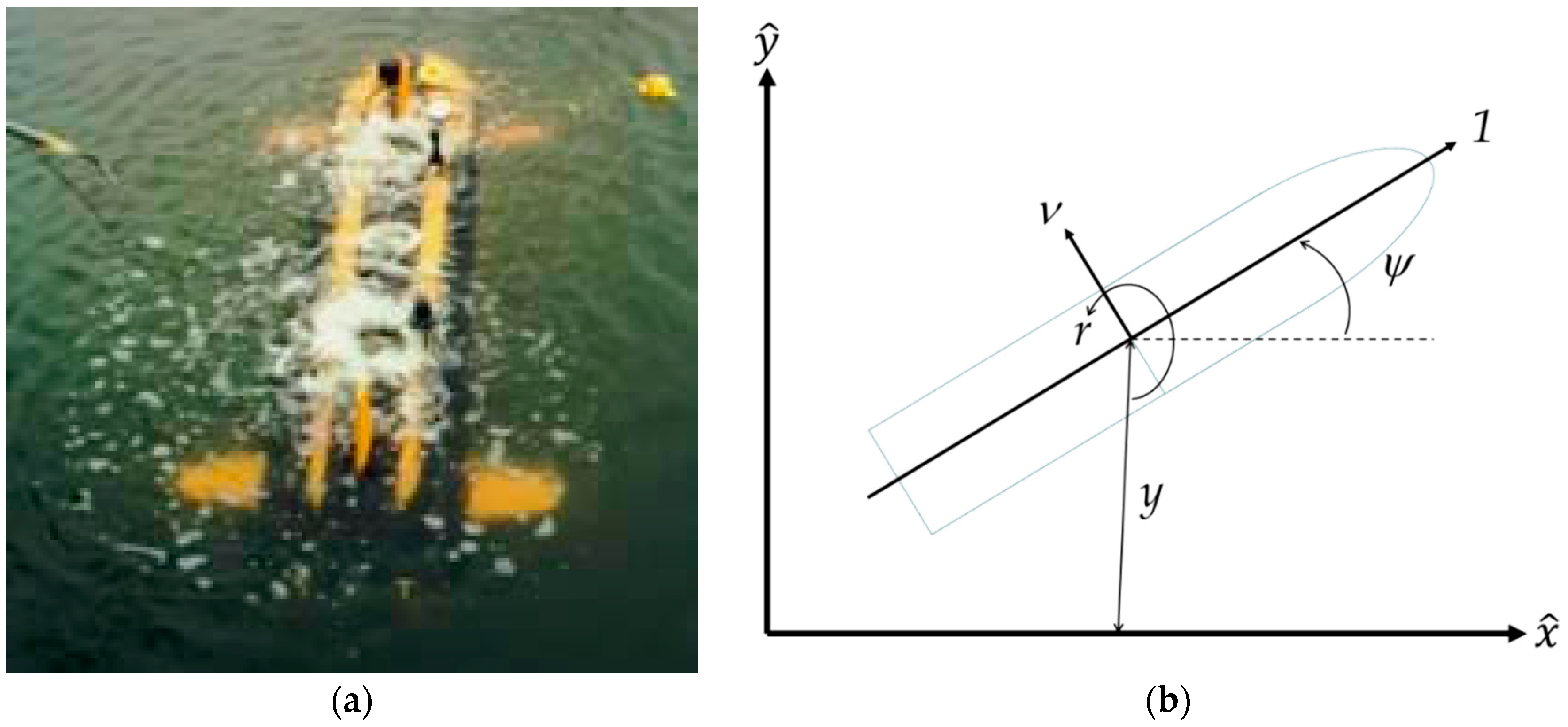
2.1. System Dynamics
| where the variables are | and the constants are | = 0.01241 | |
| ν | Lateral (sway) velocity | m = 0.0358 | = 0.01241 |
| r | Turning rate (yaw) | Iz = 0.0022 | = −0.00047 |
| ψ | Heading angle (degrees) | xG = 0.0014 | = −0.00178 |
| y | Lateral deviation (cross-track error) | = −0.00178 | = −0.00390 |
| δs | Stern rudder deflection | = −0.03430 | = −0.00769 |
| δb | Bow rudder deflection | = 0.01187 | = −0.0047 |
| = −0.10700 | = 0.0035 | ||
2.2. Control Law Design
2.3. Observer Design
2.3.1. Full-Order Observer Design
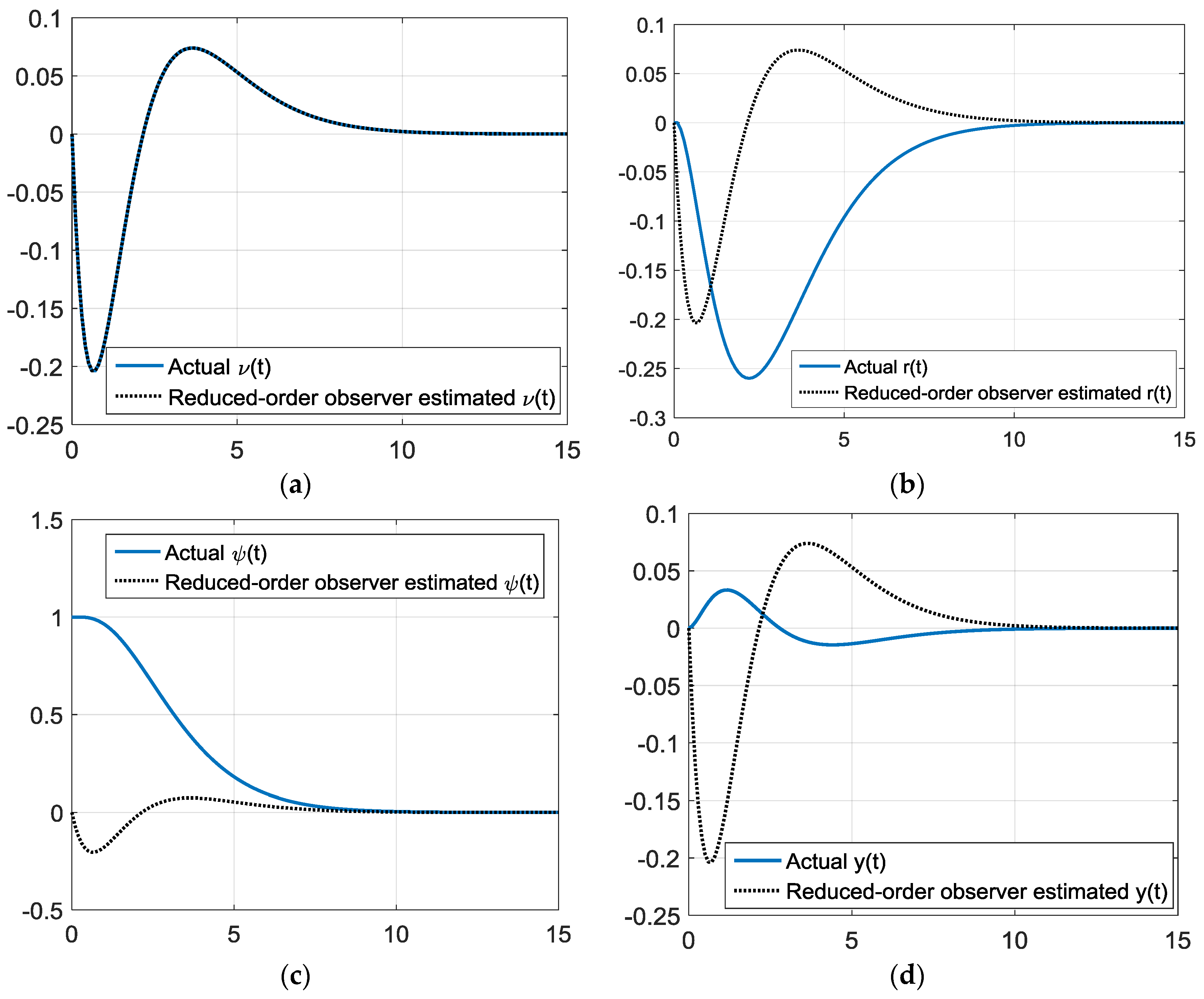
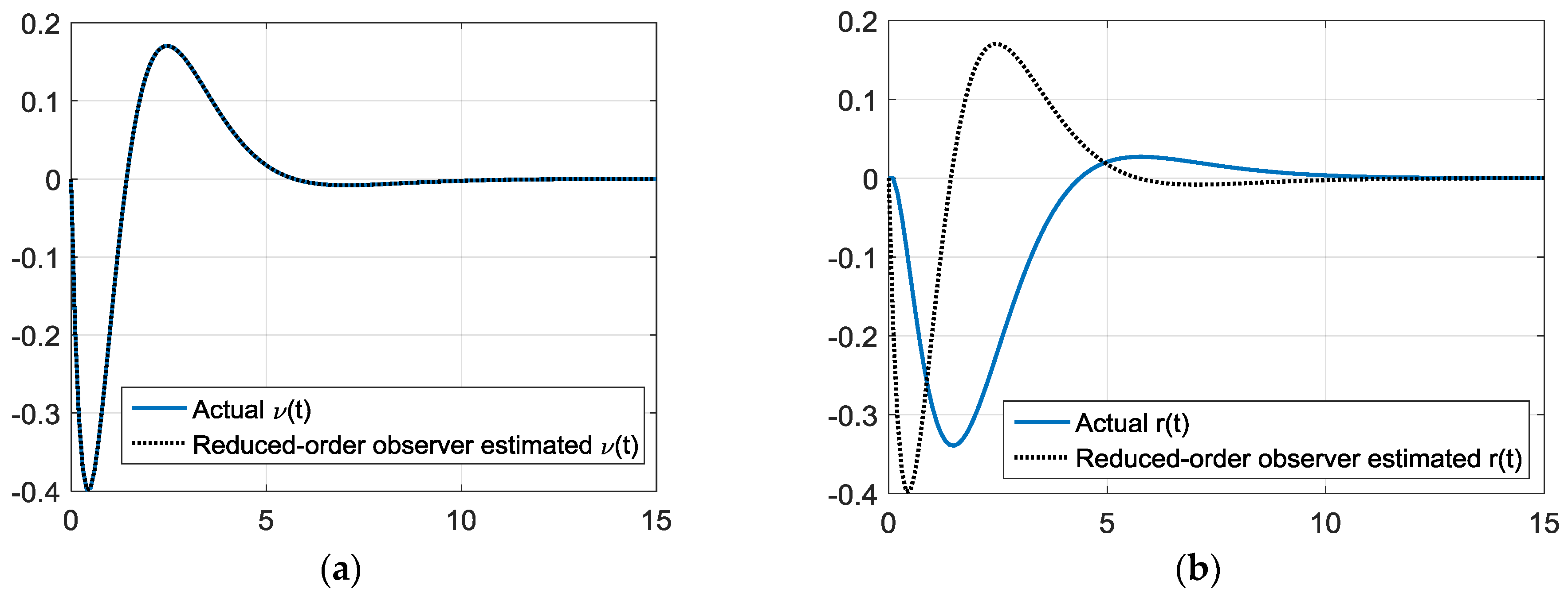
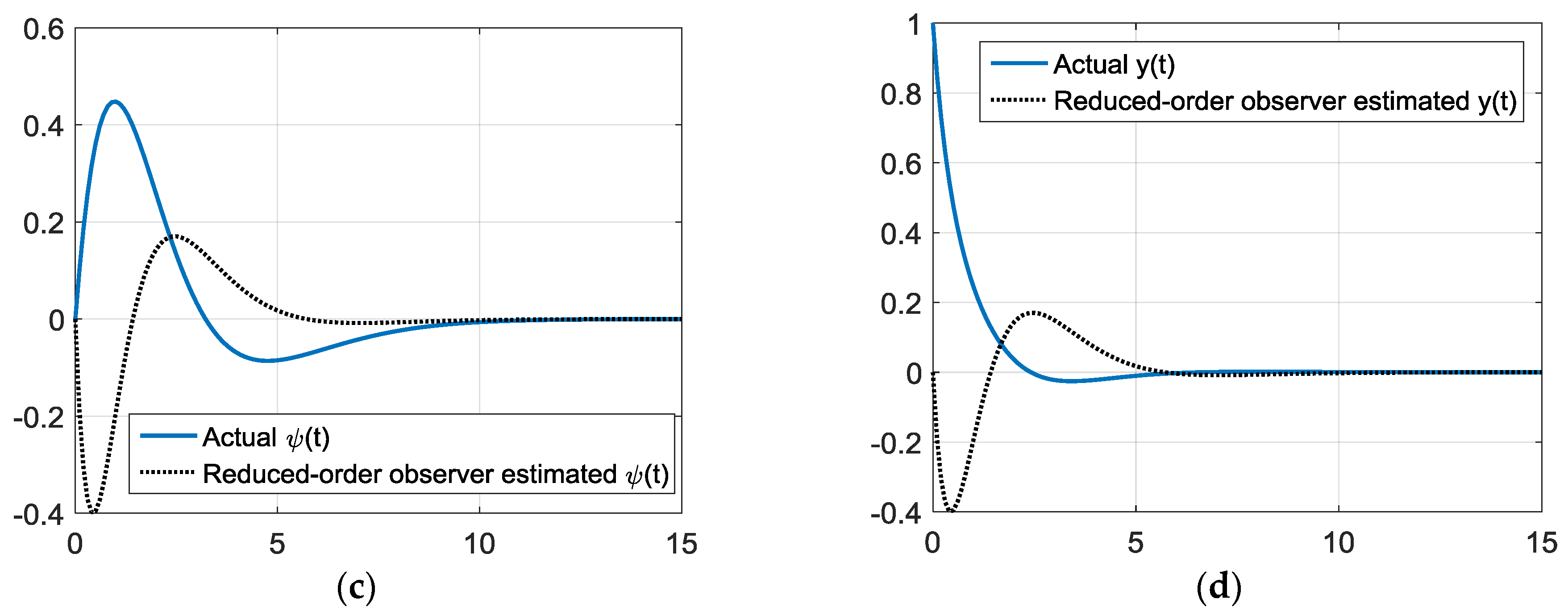
2.3.2. Reduced-Order Observer Design
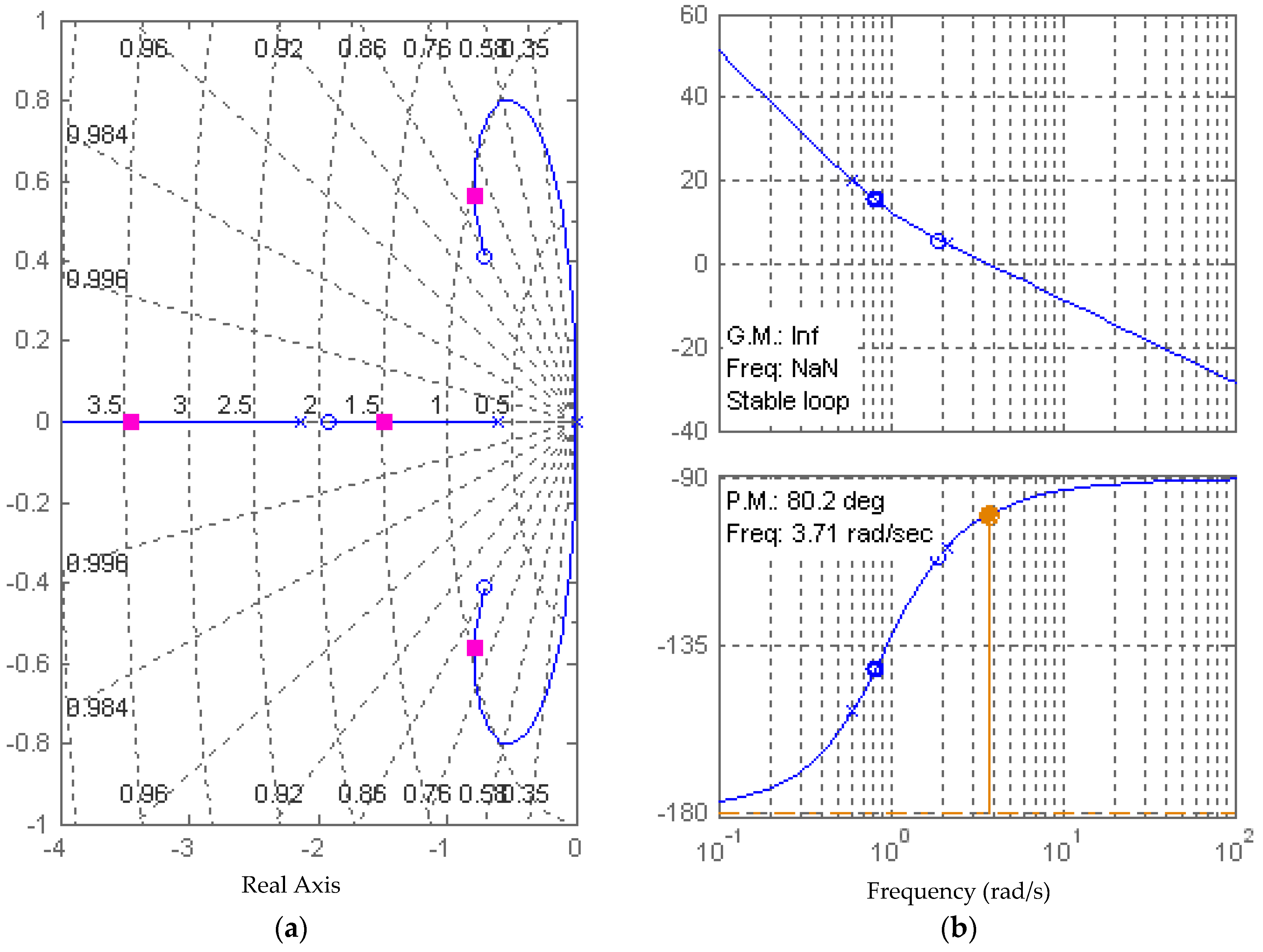
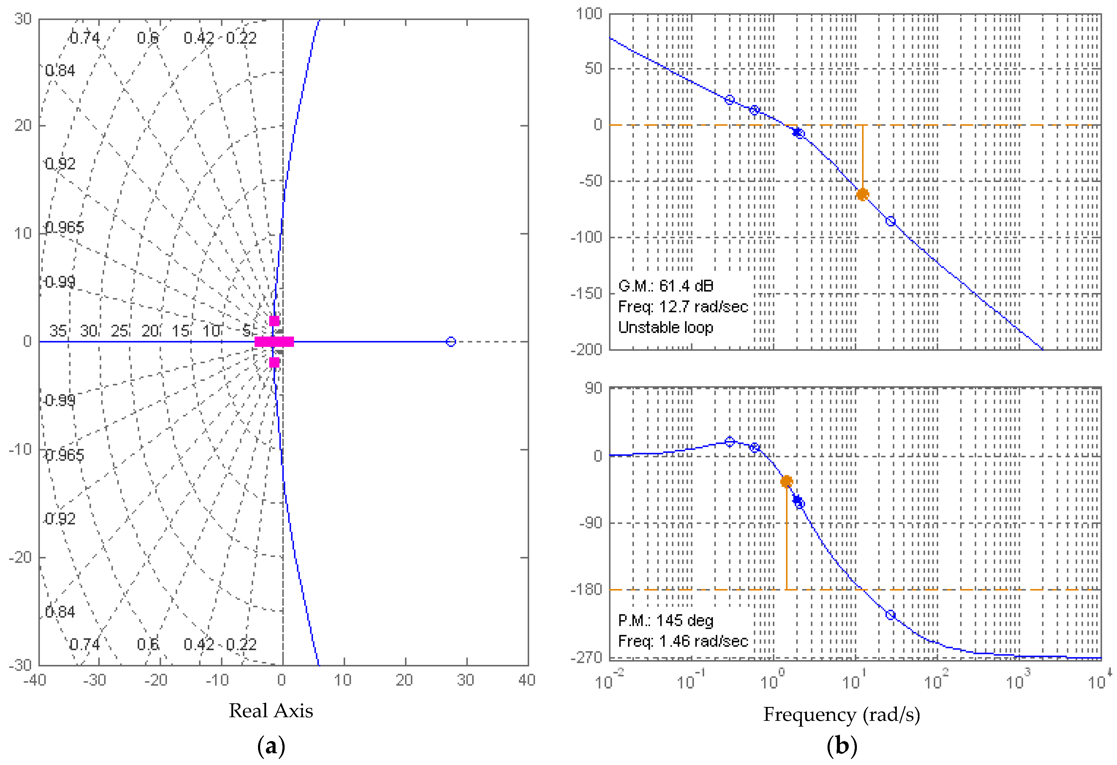
2.3.3. Gain Margin and Phase Margin
2.4. Tracking Systems and Feed-Forward Control in the Presence of Constant Disturbance Currents
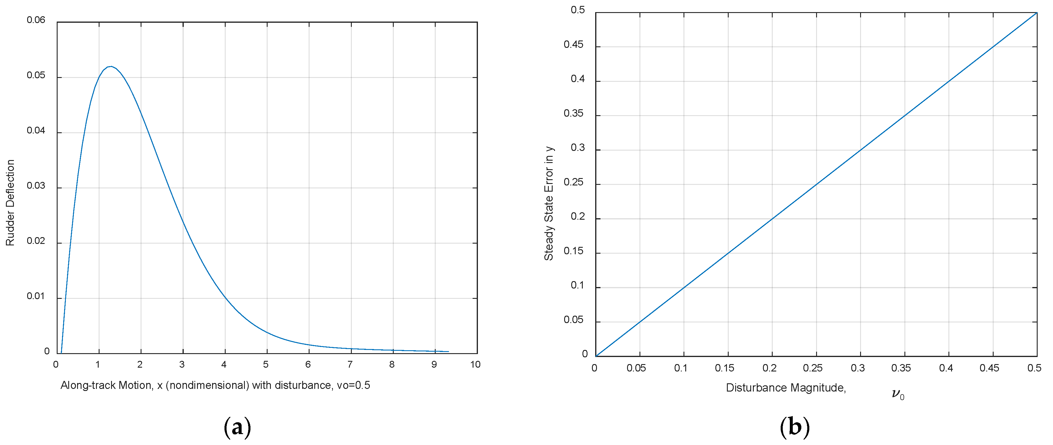
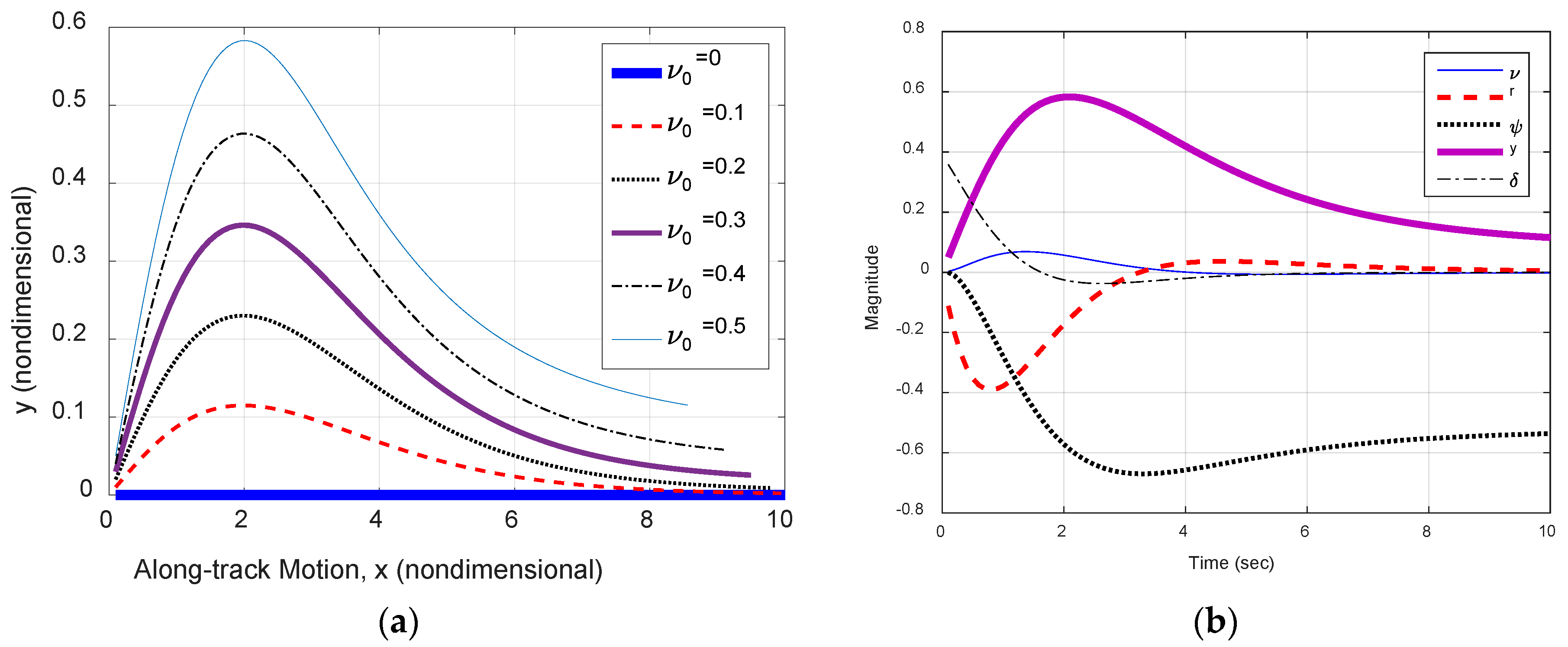
2.4.1. Analysis of Disturbed System in Ocean Currents via State Equations and Simulations
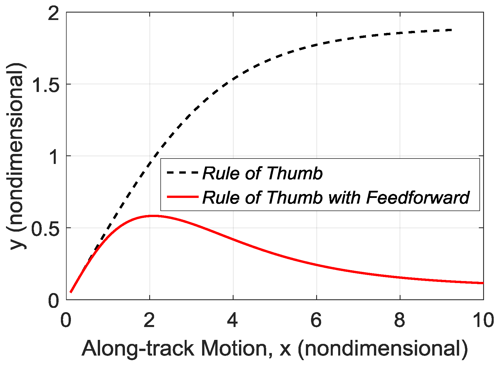
2.4.2. Elimination of Steady-State Error Using Feed-Forward Control
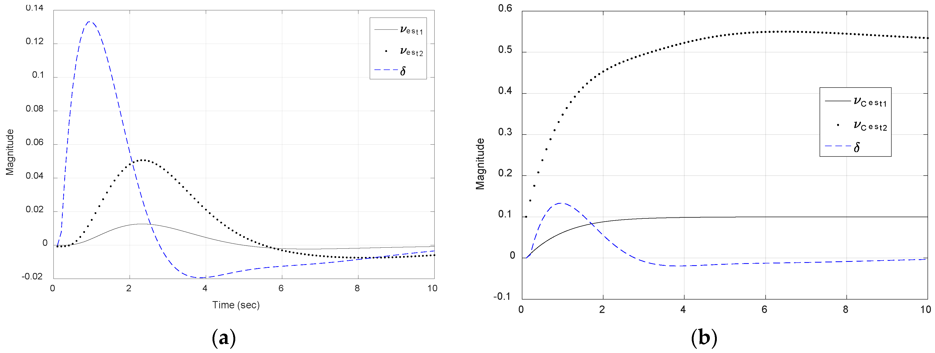
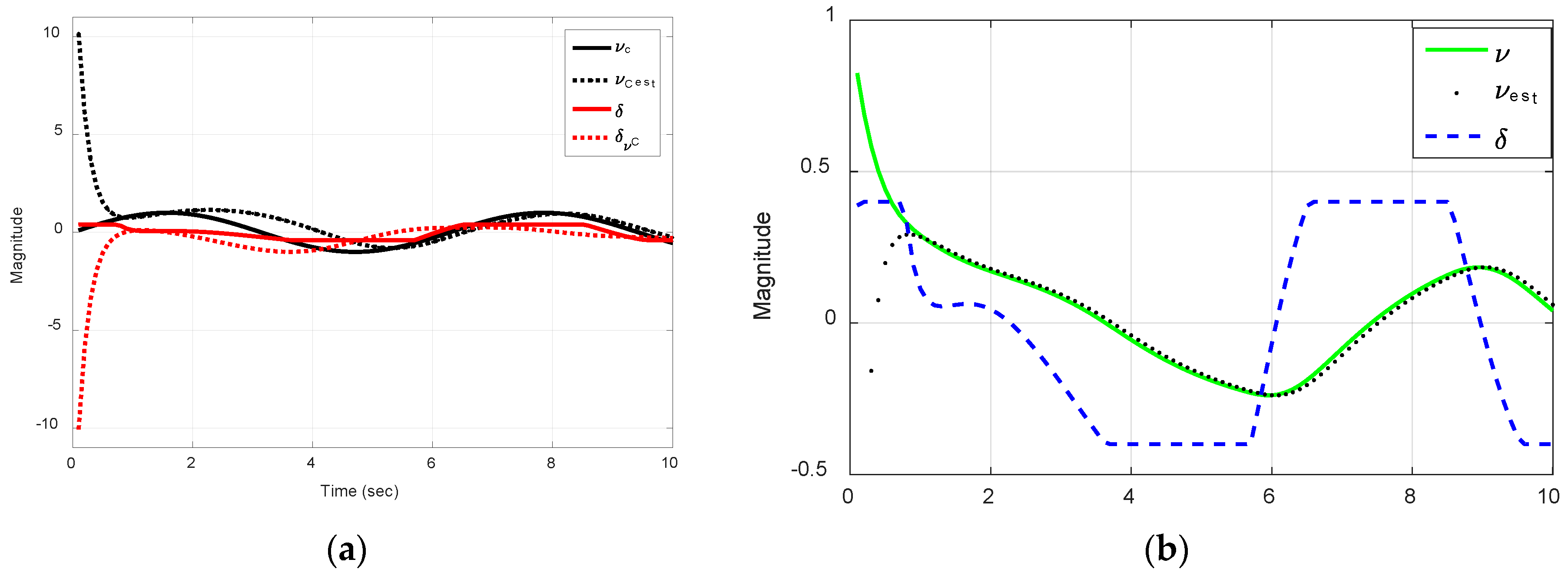
2.5. Disturbance Estimation with Reduced-Order Observer and Integral Control
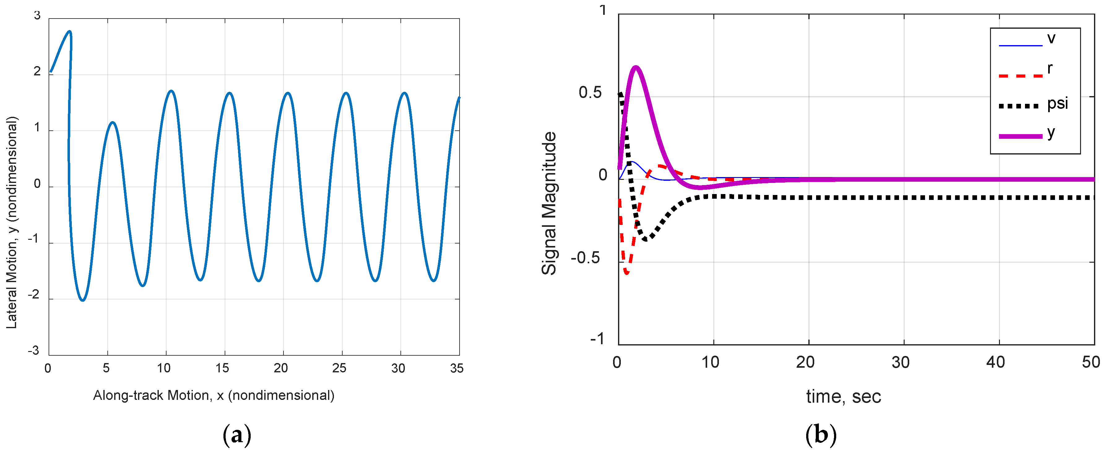
2.6. Waypoint Guidance
3. Results
3.1. System Dynamics
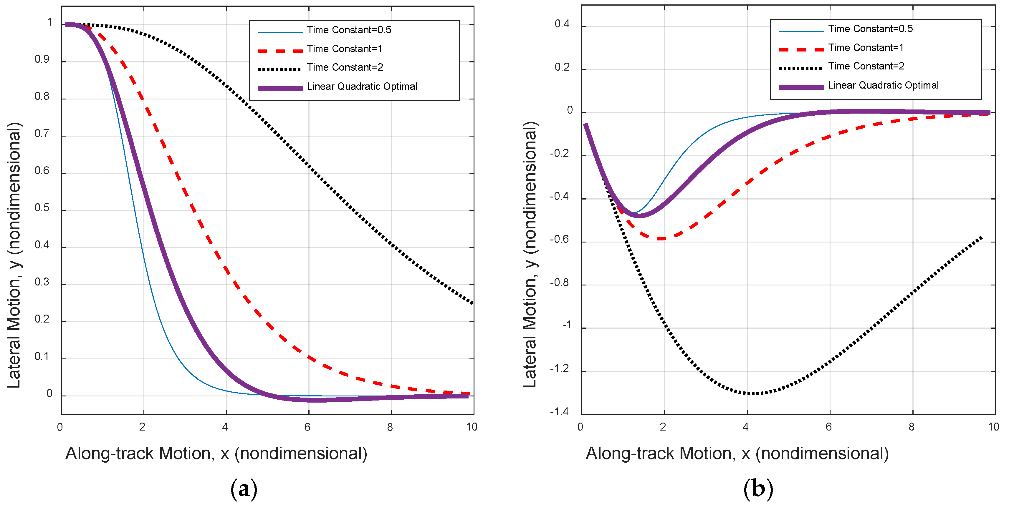
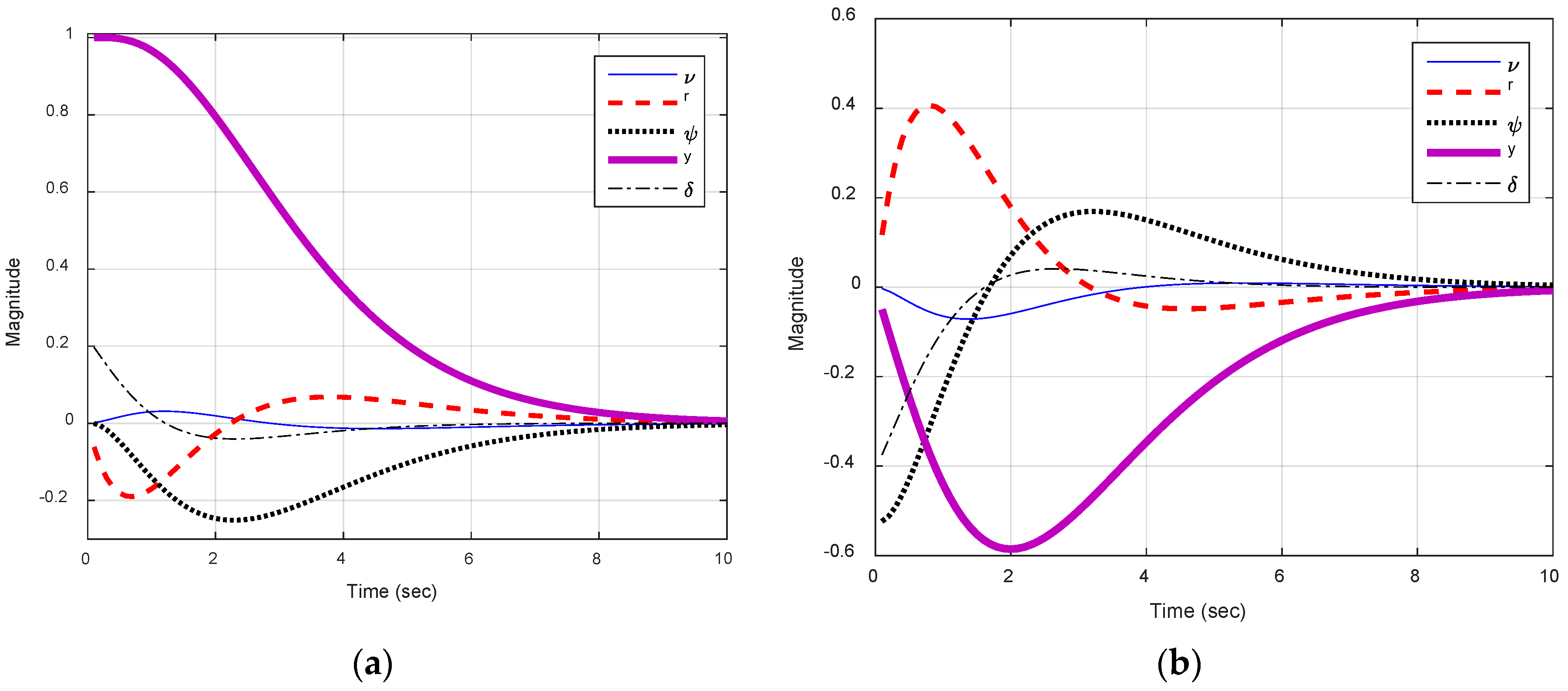
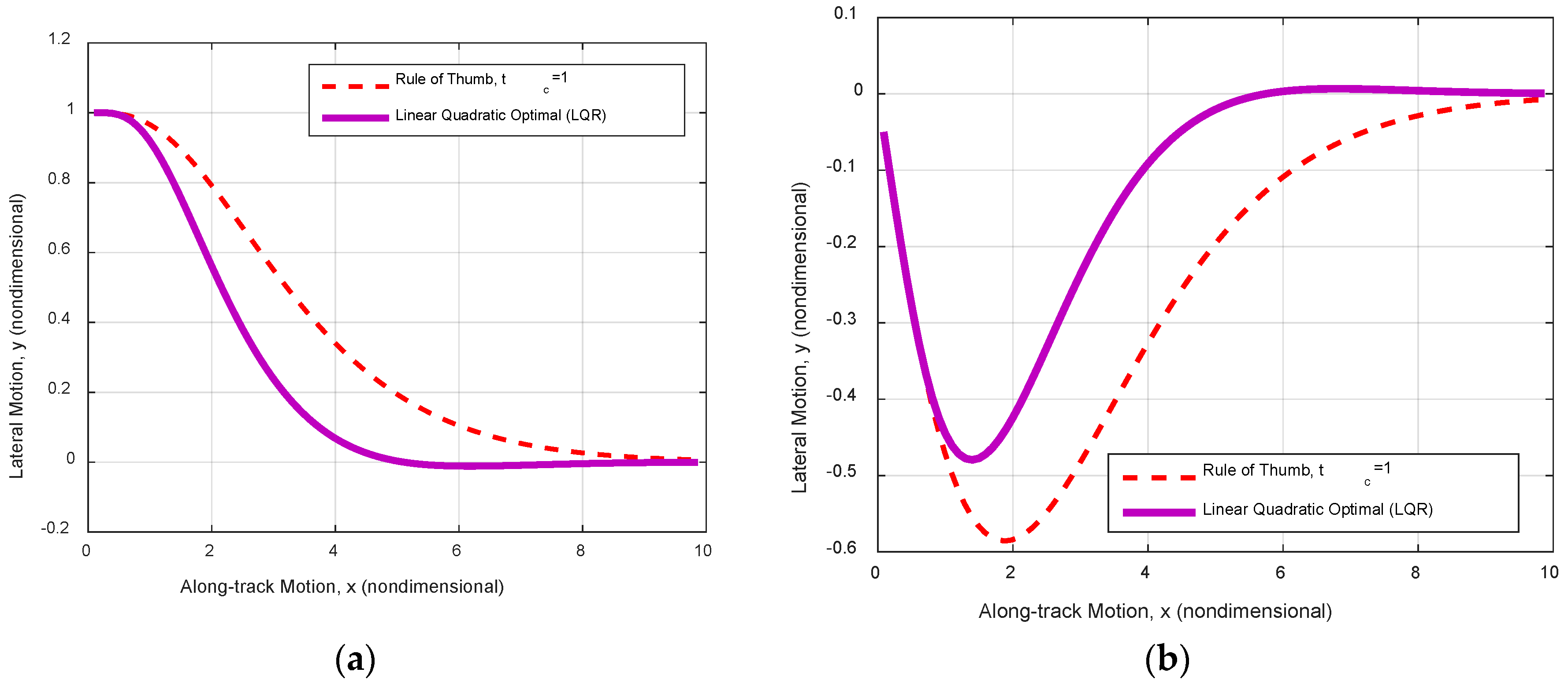
3.2. Control Law Design
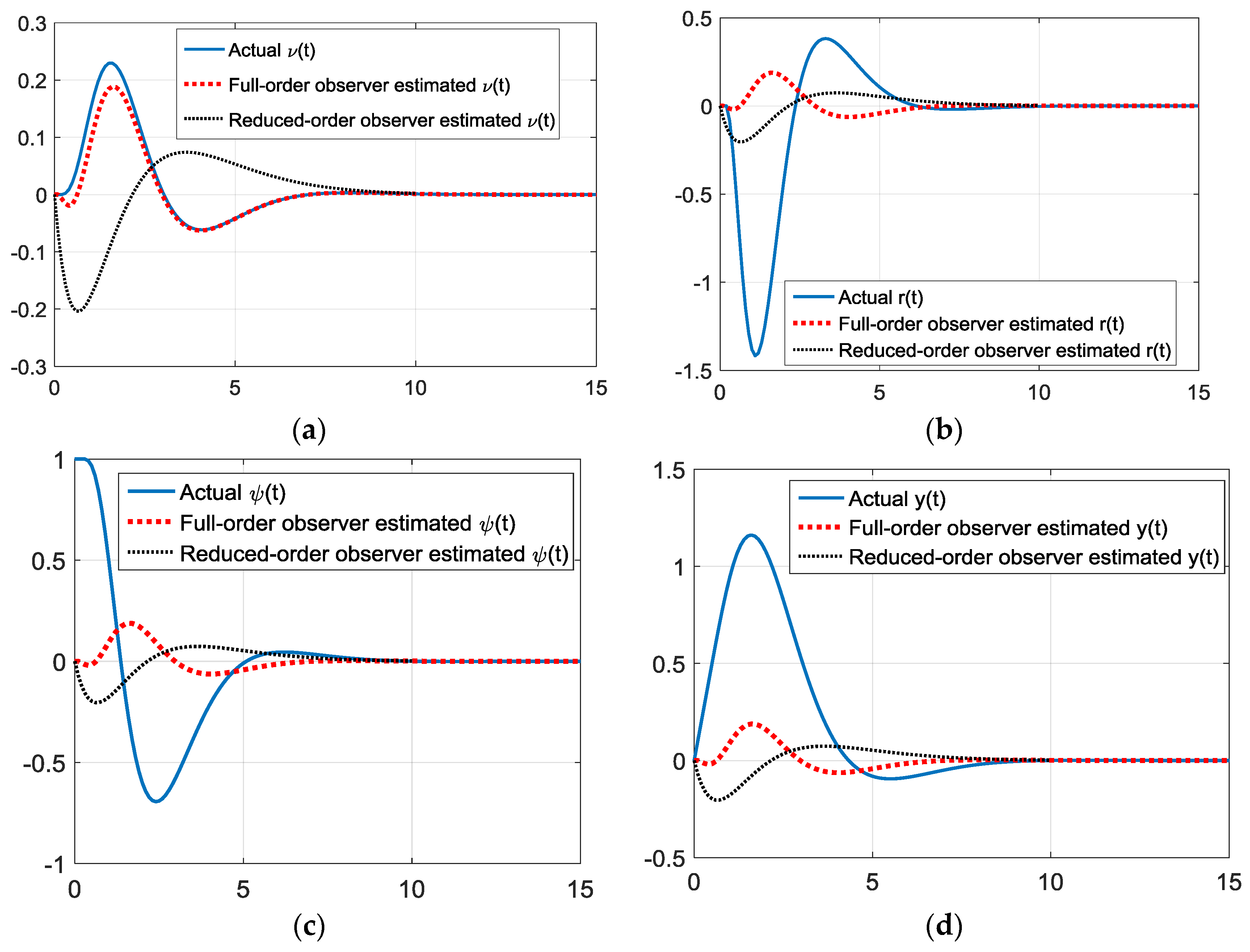
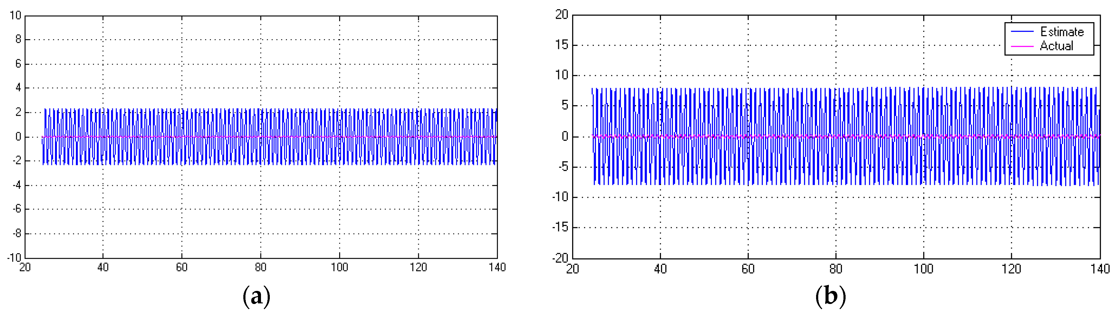
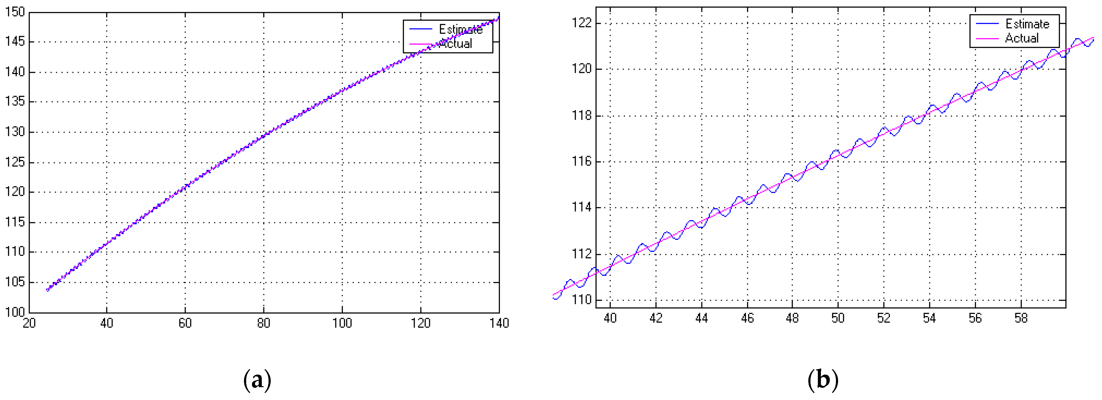
3.3. Observer Design
3.4. Tracking Systems and Feed-Forward Control in the Presence of Disturbance Currents
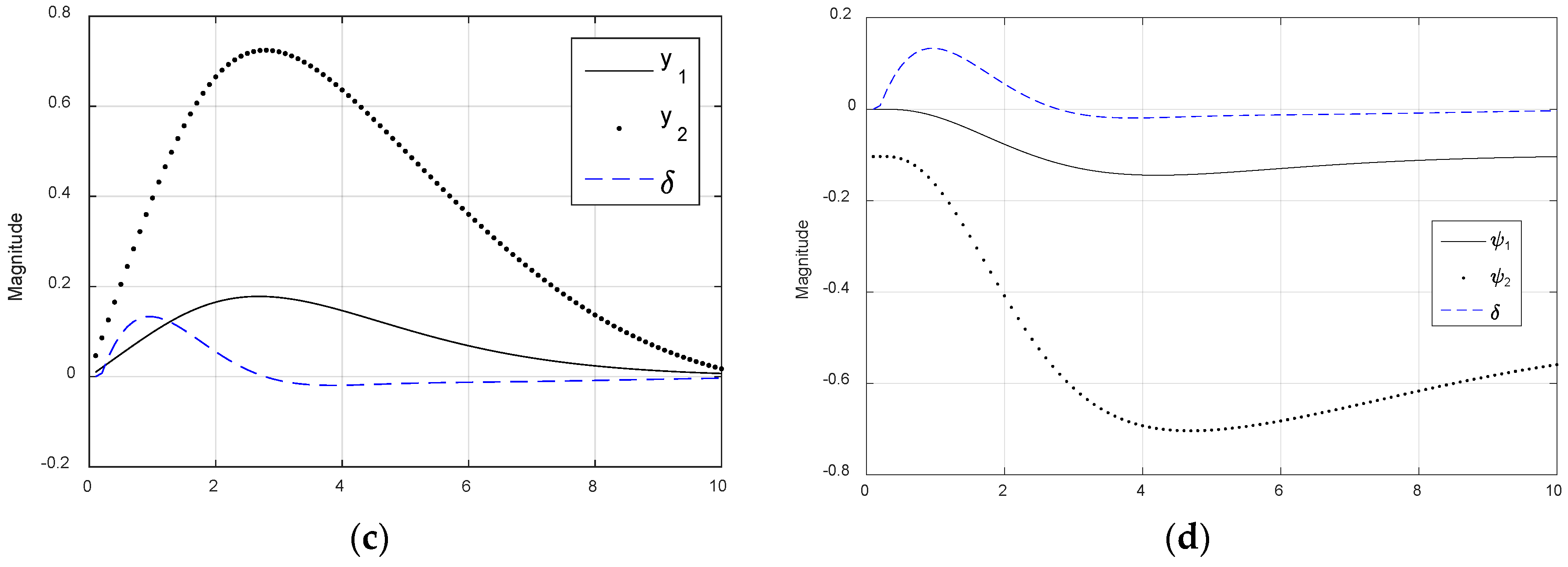
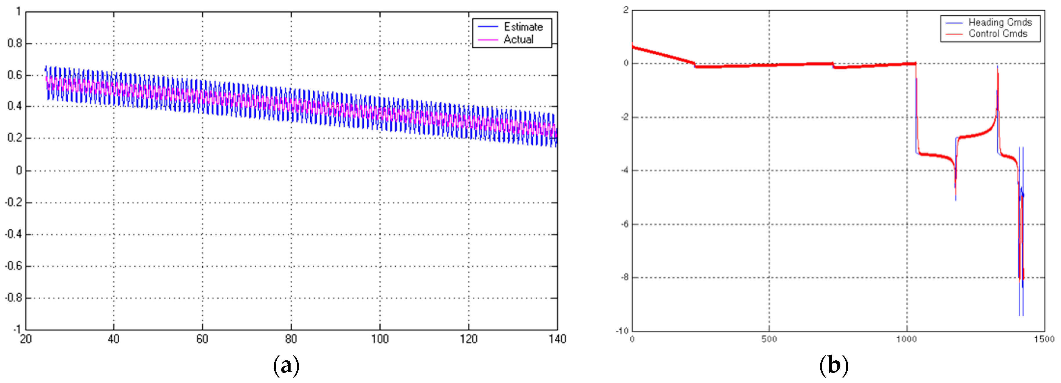
3.5. Disturbance Estimation and Integral Control
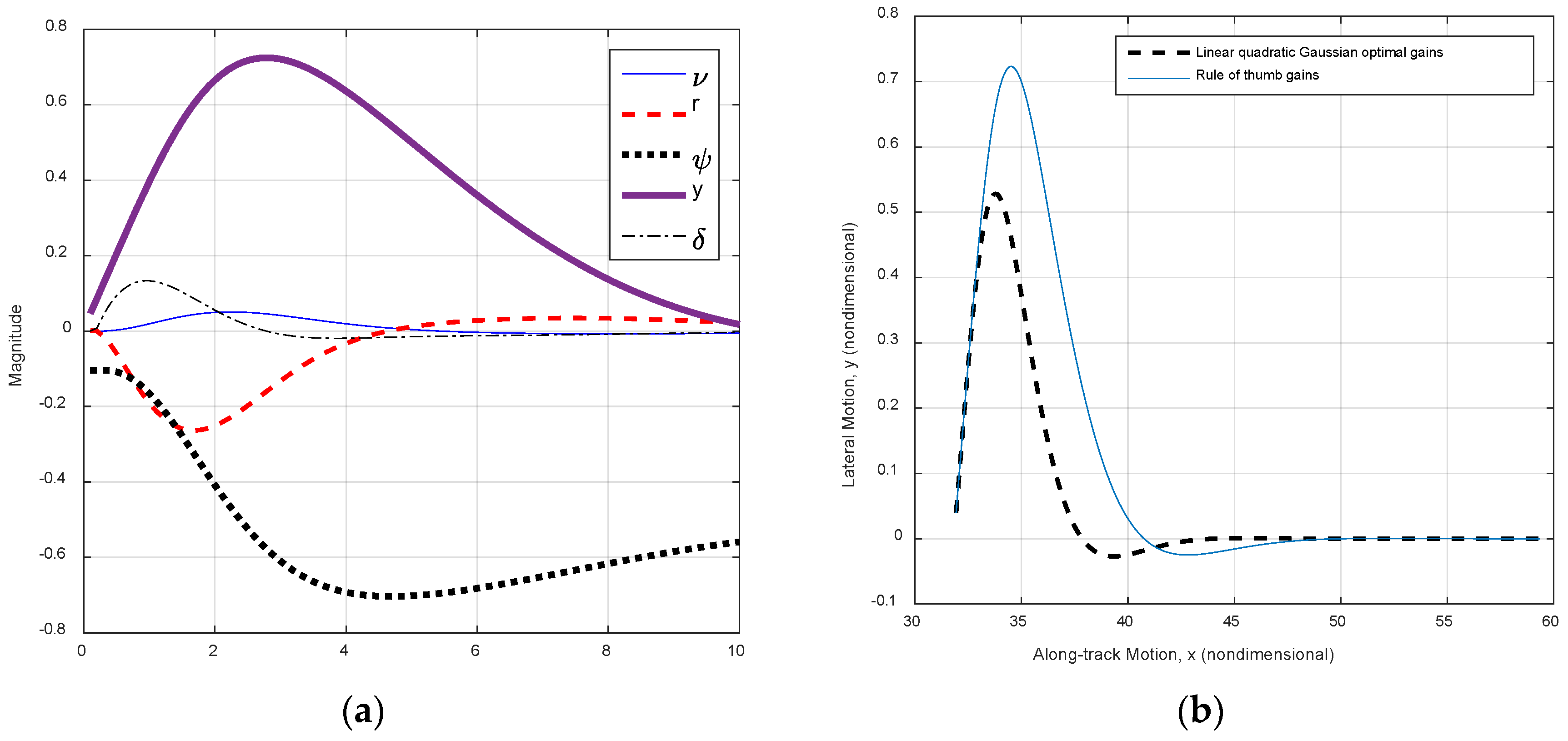
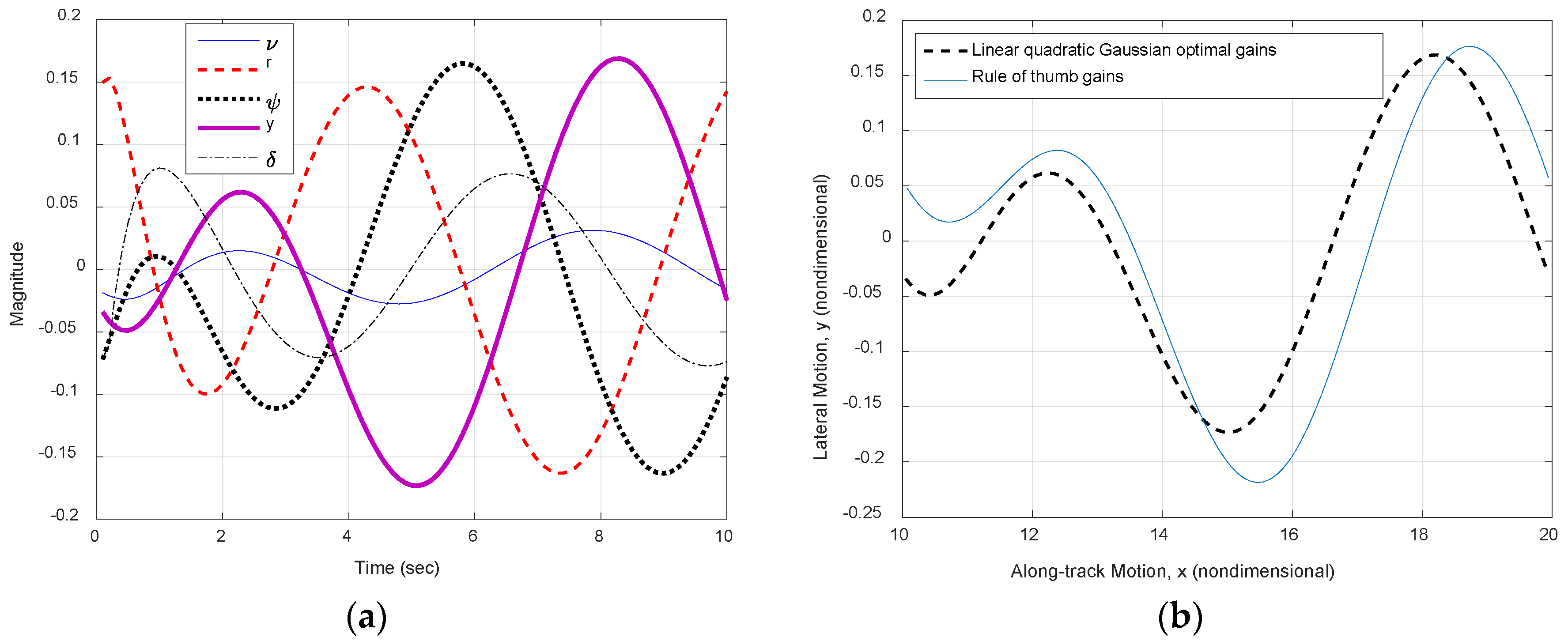
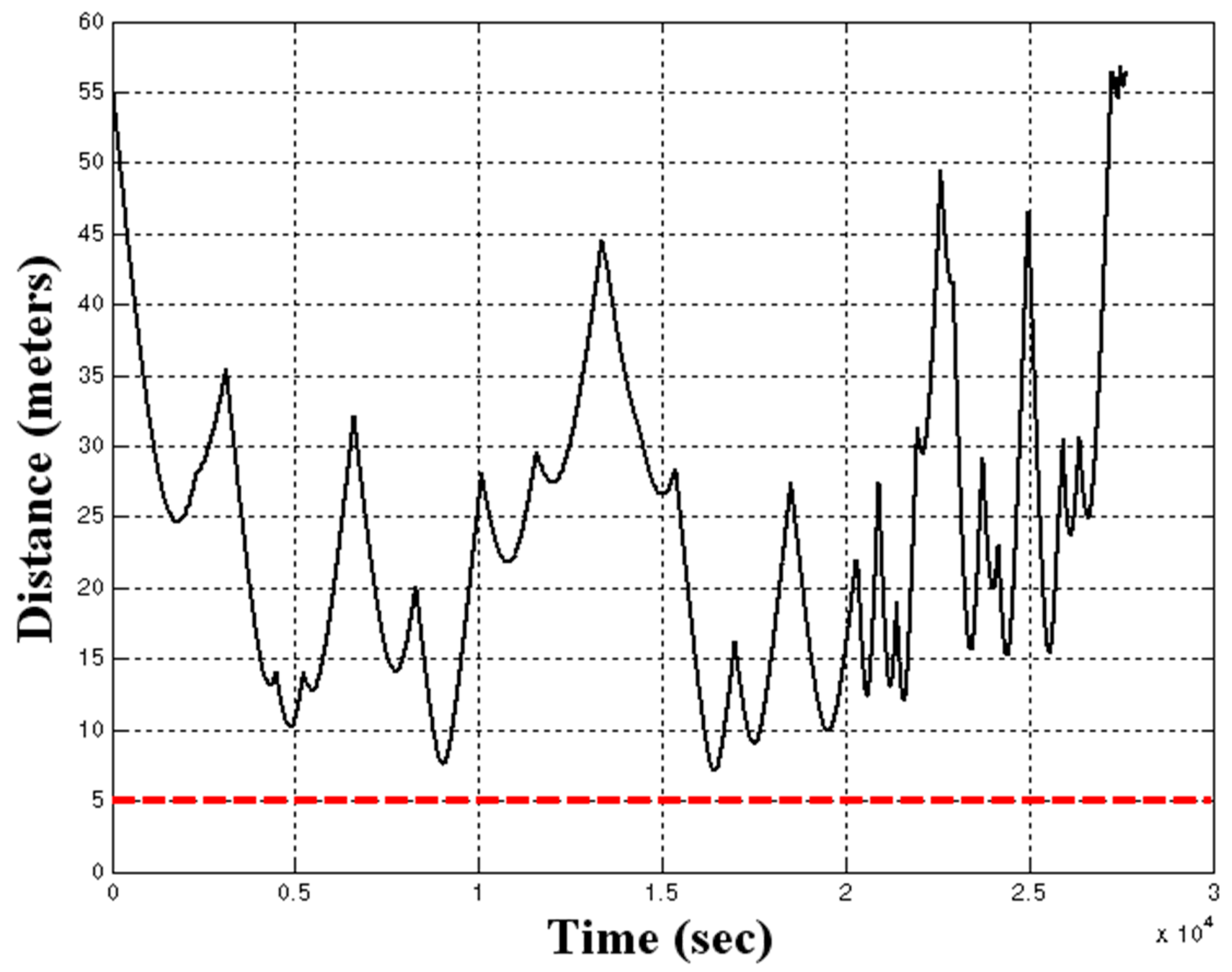
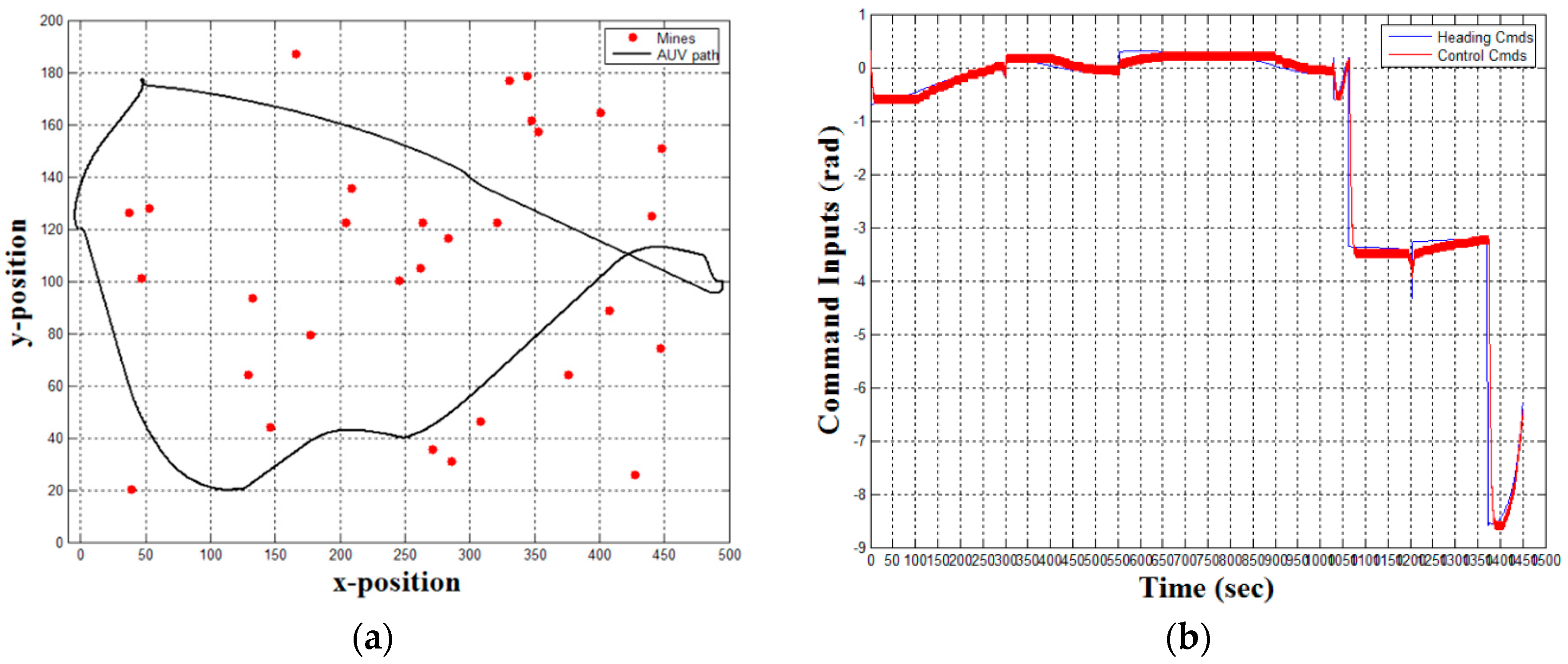
3.6. Fully-Assembled System Demonstration
4. Discussion
Author Contributions
Funding
Conflicts of Interest
References
- Naval Postgraduate School Website for Consortium for Robotics and Unmanned Systems Education and Research (CRUSER). Available online: http://auvac.org/people-organizations/view/241 (accessed on 23 May 2018).
- Brutzman, D.; Healey, A.J.; Marco, D.B.; McGhee, R.B. The Phoenix Autonomous Underwater Vehicle. In AI Based Mobile Robots; Kortenkamp, D., Bonasso, R.P., Murphy, R.R., Eds.; MIT/AAAI Press: Cambridge, MA, USA, 1998. [Google Scholar]
- Naval Postgraduate School Website for Consortium for Robotics and Unmanned Systems Education and Research (CRUSER). Available online: https://my.nps.edu/web/cavr/auv (accessed on 23 May 2018).
- Ogata, K. Modern Control Engineering, 4th ed.; Prentice-Hall: Upper Saddle River, NJ, USA, 2002; pp. 779–790. ISBN 0-13-060907-2. [Google Scholar]
- Marco, D.B.; Healey, A.J. Surge Motion Parameter Identification for the NPS Phoenix AUV. In Proceedings International Advanced Robotics Program IARP 98; University of South Louisiana: Baton Rouge, LA, USA, 1998; pp. 197–210. [Google Scholar]
- Kenny, T.; Sands, T. Experimental piezoelectric system identification. J. Mech. Eng. Autom. 2017, 76, 179–195. [Google Scholar] [CrossRef]
- Sands, T. Nonlinear-adaptive mathematical system identification. Computation 2017, 5, 47–59. [Google Scholar] [CrossRef]
- Kenny, T.; Sands, T. Experimental Sensor Characterization. J. Space Explor. 2017, 7, 140. [Google Scholar]
- Sands, T. Space System Identification Algorithms. J. Space Explor. 2017, 6, 138. [Google Scholar]
- Armani, C.; Sands, T. Analysis, correlation, and estimation for control of material properties. J. Mech. Eng. Autom. 2018, 8, 7–31. [Google Scholar] [CrossRef]
- Wu, N.; Wu, C.; Ge, T.; Yang, D.; Yang, R. Pitch Channel Control of a REMUS AUV with Input Saturation and Coupling Disturbances. Appl. Sci. 2018, 8, 253. [Google Scholar] [CrossRef]
- He, B.; Zhang, H.; Li, C.; Zhang, S.; Liang, Y.; Yan, T. Autonomous Navigation for Autonomous Underwater Vehicles Based on Information Filters and Active Sensing. Sensors 2011, 11, 10958–10980. [Google Scholar] [CrossRef] [PubMed]
- Yan, Z.; Wang, L.; Zhang, W.; Zhou, J.; Wang, M. Polar Grid Navigation Algorithm for Unmanned Underwater Vehicles. Sensors 2017, 17, 1599. [Google Scholar] [CrossRef]
- Wang, J.; Li, B.; Chen, L.; Li, L. A Novel Detection Method for Underwater Moving Targets by Measuring Their ELF Emissions with Inductive Sensors. Sensors 2017, 17, 1734. [Google Scholar] [CrossRef] [PubMed]
- Eren, F.; Pe’eri, S.; Thein, M.; Rzhanov, Y.; Celikkol, B.; Swift, M.R. Position, Orientation and Velocity Detection of Unmanned Underwater Vehicles (UUVs) Using an Optical Detector Array. Sensors 2017, 17, 1741. [Google Scholar] [CrossRef] [PubMed]
- Zhang, W.; Wei, S.; Teng, Y.; Zhang, J.; Wang, X.; Yan, Z. Dynamic Obstacle Avoidance for Unmanned Underwater Vehicles Based on an Improved Velocity Obstacle Method. Sensors 2017, 17, 2742. [Google Scholar] [CrossRef] [PubMed]
- Kim, J.J.; Agrawal, B.; Sands, T. 2H Singularity free momentum generation with non-redundant control moment gyroscopes. In Proceedings of the 45th IEEE Conference on Decision and Control, San Diego, CA, USA, 13–15 December 2006; pp. 1551–1556. [Google Scholar] [CrossRef]
- Kim, J.J.; Agrawal, B.; Sands, T. Control moment gyroscope singularity reduction via decoupled control. In Proceedings of the IEEE Southeastcon 2009, Atlanta, GA, USA, 5–8 March 2009; pp. 1551–1556. [Google Scholar] [CrossRef]
- Sands, T.; Kim, J.J.; Agrawal, B. Nonredundant single-gimbaled control moment gyroscopes. J. Guid. Control Dyn. 2012, 35, 578–587. [Google Scholar] [CrossRef]
- Kim, J.J.; Agrawal, B.; Sands, T. Experiments in Control of Rotational Mechanics. Int. J. Autom. Control. Intell. Syst. 2016, 2, 9–22. [Google Scholar]
- Agrawal, B.; Kim, J.J.; Sands, T. Method and Apparatus for Singularity Avoidance for Control Moment Gyroscope (CMG) Systems without Using Null Motion. U.S. Patent 9,567,112, 2017. [Google Scholar]
- Agrawal, B.; Kim, J.J.; Sands, T. Singularity Penetration with Unit Delay (SPUD). Mathematics 2018, 6, 23–38. [Google Scholar] [CrossRef]
- Lu, D.; Chu, J.; Cheng, B.; Sands, T. Developments in angular momentum exchange. Int. J. Aerosp. Sci. 2018, 6, 1–7. [Google Scholar] [CrossRef]
- Thornton, B.; Ura, T.; Nose, Y. Wind-up AUVs Combined energy storage and attitude control using control moment gyros. In Proceedings of the Oceans 2007, Vancouver, BC, Canada, 29 September–4 October 2007. [Google Scholar] [CrossRef]
- Thornton, B.; Ura, T.; Nose, Y. Combined energy storage and three-axis attitude control of a gyroscopically actuated AUV. In Proceedings of the Oceans 2008, Quebec City, QC, Canada, 15–18 September 2008. [Google Scholar] [CrossRef]
- Sands, T. Strategies for combating Islamic state. Soc. Sci. 2016, 5, 39. [Google Scholar] [CrossRef]
- Mihalik, R.; Sands, T. Outcomes of the 2010 and 2015 nonproliferation treaty review conferences. World J. Soc. Sci. Humanit. 2016, 2, 46–51. [Google Scholar] [CrossRef]
- Camacho, H.; Mihalik, R.; Sands, T. Education in Nuclear Deterrence and Assurance. J. Def. Manag. 2017, 7, 166. [Google Scholar] [CrossRef]
- Mihalik, R.; Camacho, H.; Sands, T. Continuum of learning: Combining education, training and experiences. Education 2017, 8, 9–13. [Google Scholar] [CrossRef]
- Camacho, H.; Mihalik, R.; Sands, T. Theoretical Context of the Nuclear Posture Review. J. Soc. Sci. 2018, 14, 124–128. [Google Scholar] [CrossRef]
- Mihalik, R.; Camacho, H.; Sands, T.U.S. Nuclear Posture Review—Kahn vs. Schelling. Soc. Sci. 2018, 14, 145–154. [Google Scholar]
- Sands, T. Physics-based control methods. In Advances in Spacecraft Systems and Orbit Determination; InTech: London, UK, 2012. [Google Scholar]
- Nakatani, S.; Sands, T. Simulation of spacecraft damage tolerance and adaptive controls. In Proceedings of the 2014 IEEE Aerospace Conference, Big Sky, MT, USA, 1–8 March 2014; pp. 1–16. [Google Scholar] [CrossRef]
- Nakatani, S.; Sands, T. Autonomous damage recovery in space. Int. J. Autom. Control. Intell. Syst. 2016, 2, 22–36. [Google Scholar]
- Cooper, M.; Heidlauf, P.; Sands, T. Controlling Chaos—Forced van der Pol Equation. Mathematics 2017, 5, 70–80. [Google Scholar] [CrossRef]
- Nakatani, S.; Sands, T. Battle-damage tolerant automatic controls. Elec. Electr. Eng. 2018, 8, 10–23. [Google Scholar] [CrossRef]
- Sands, T. Satellite electronic attack of enemy air defenses. In Proceedings of the IEEE Southeastcon 2009, Atlanta, GA, USA, 5–8 March 2009; pp. 434–438. [Google Scholar] [CrossRef]
- Sands, T. Space mission analysis and design for electromagnetic suppression of radar. Int. J. Electromagn. Appl. 2018, 8, 1–25. [Google Scholar] [CrossRef]
- Nakatani, S.; Sands, T. Eliminating the existential threat from North Korea. Sci. Technol. 2018, 8, 11–16. [Google Scholar] [CrossRef]
- Smeresky, B.; Rizzo, A.; Sands, T. Kinematics in the Information Age. Mathematics 2018. accepted. [Google Scholar]


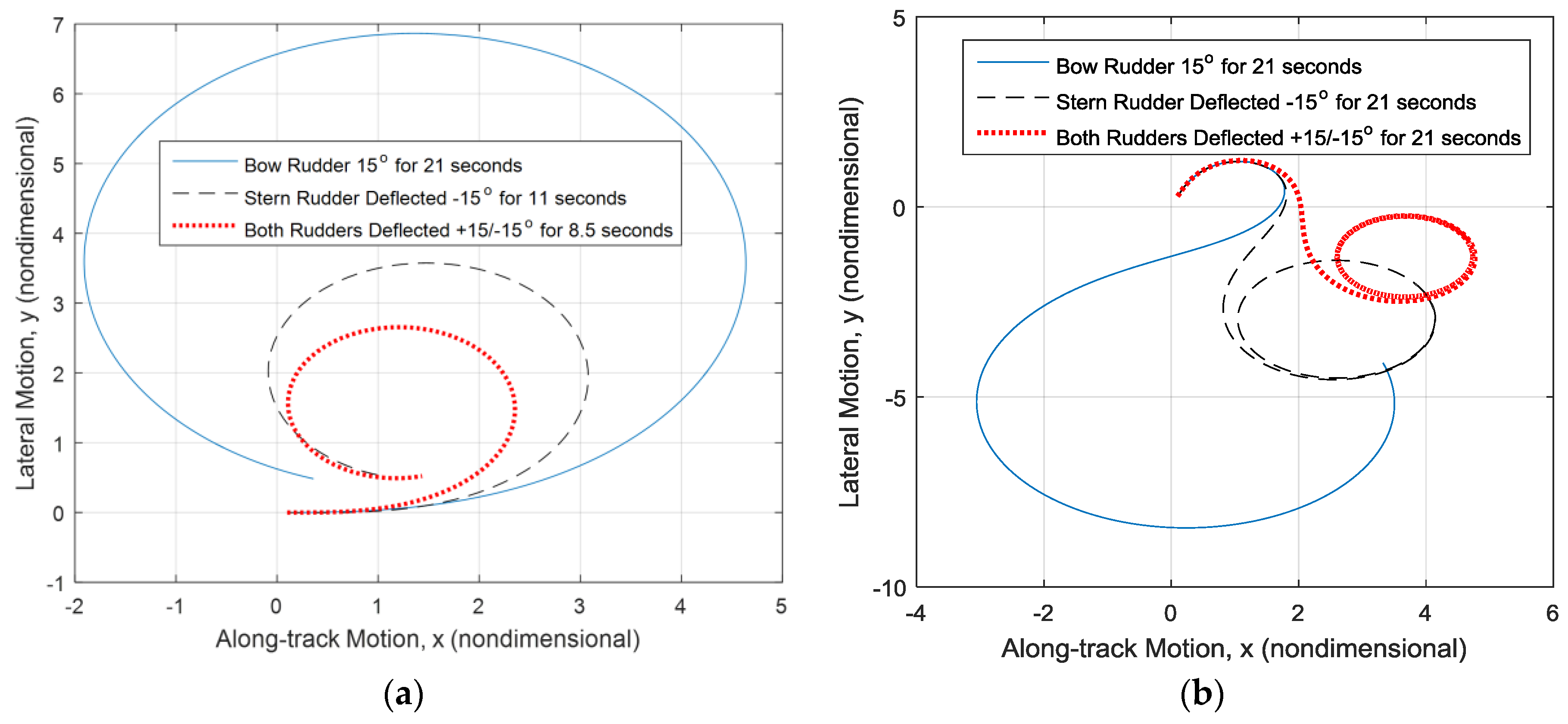
| Rudder Deflected | Euler: x-Distance 1 | Runge-Kutte: x-Distance 1 | Euler: y-Distance 1 | Runge-Kutte: y-Distance 1 |
|---|---|---|---|---|
| Bow | 6.5471 | 6.5469 | 6.8647 | 6.8646 |
| Stern | 3.1665 | 3.1665 | 3.5768 | 3.5768 |
| Both | 2.4546 | 2.4546 | 2.6567 | 2.6567 |
| Time Constant | ||||
|---|---|---|---|---|
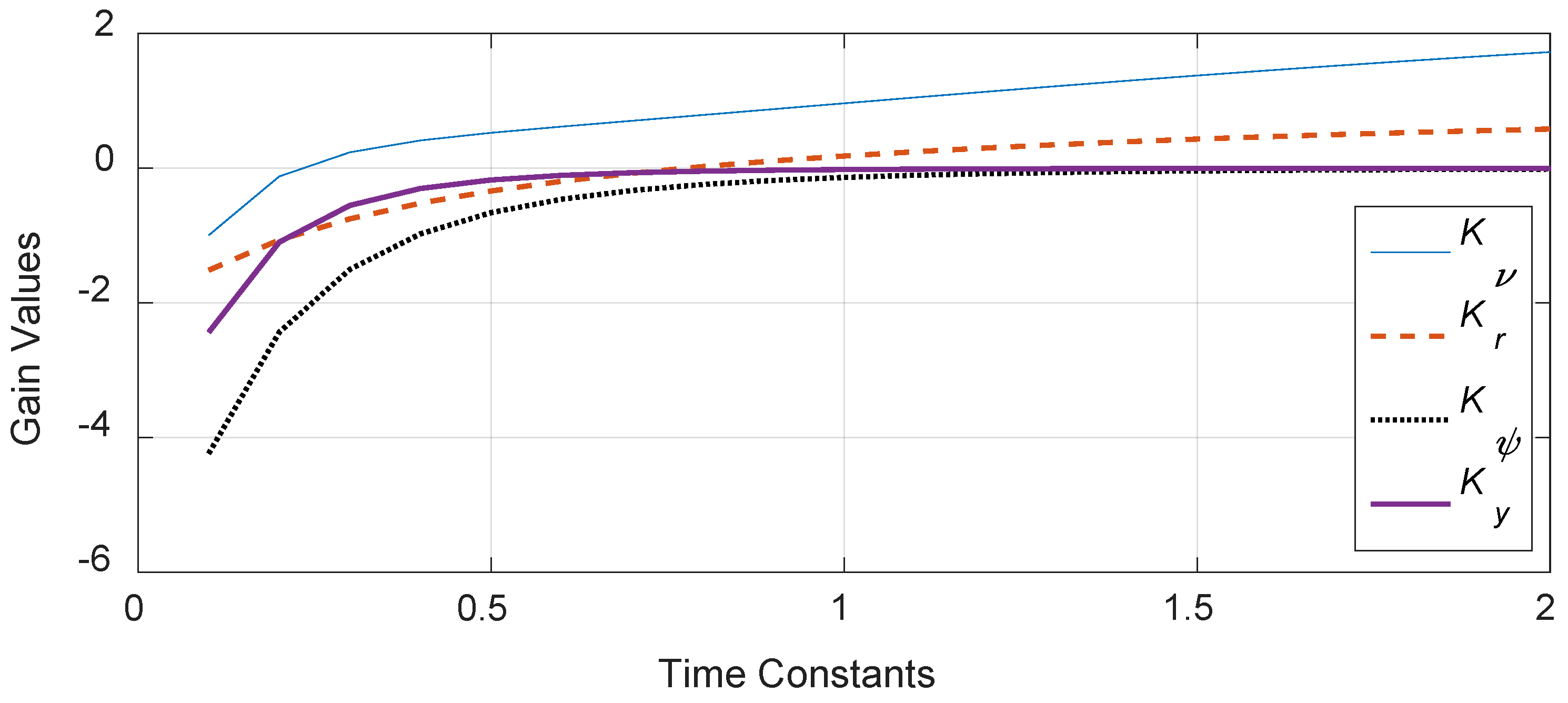
| 0.5 | −1.5135 | −1.7005 | −5.1508 | −3.22524 |
| 1 | 0.5070 | −0.3687 | −0.7157 | −0.1972 |
| 2 | 1.1248 | 0.2870 | −0.0906 | −0.0116 |
| LQR | −0.0939 | −1.2043 | −2.2138 | −1 |
| Multiple of the Controller Time Constant Used for the Observer | Observer Gain Matrix |
|---|---|
| 1 | |
| Sensors Used to Measure States | Observability Matrix Condition Number 1 |
|---|---|
| and | 8.8456 |
| and | 21.1306 |
| and | 31.2919 |
| Multiple of the Controller Time Constant Used for Observer | Observer Gain Matrix |
|---|---|
| 1 | |
© 2018 by the authors. Licensee MDPI, Basel, Switzerland. This article is an open access article distributed under the terms and conditions of the Creative Commons Attribution (CC BY) license (http://creativecommons.org/licenses/by/4.0/).
Share and Cite
Sands, T.; Bollino, K.; Kaminer, I.; Healey, A. Autonomous Minimum Safe Distance Maintenance from Submersed Obstacles in Ocean Currents. J. Mar. Sci. Eng. 2018, 6, 98. https://doi.org/10.3390/jmse6030098
Sands T, Bollino K, Kaminer I, Healey A. Autonomous Minimum Safe Distance Maintenance from Submersed Obstacles in Ocean Currents. Journal of Marine Science and Engineering. 2018; 6(3):98. https://doi.org/10.3390/jmse6030098
Chicago/Turabian StyleSands, Timothy, Kevin Bollino, Isaac Kaminer, and Anthony Healey. 2018. "Autonomous Minimum Safe Distance Maintenance from Submersed Obstacles in Ocean Currents" Journal of Marine Science and Engineering 6, no. 3: 98. https://doi.org/10.3390/jmse6030098
APA StyleSands, T., Bollino, K., Kaminer, I., & Healey, A. (2018). Autonomous Minimum Safe Distance Maintenance from Submersed Obstacles in Ocean Currents. Journal of Marine Science and Engineering, 6(3), 98. https://doi.org/10.3390/jmse6030098