Modelling Hydrodynamic Impacts of Sea-Level Rise on Wave-Dominated Australian Estuaries with Differing Geomorphology


Abstract
1. Introduction
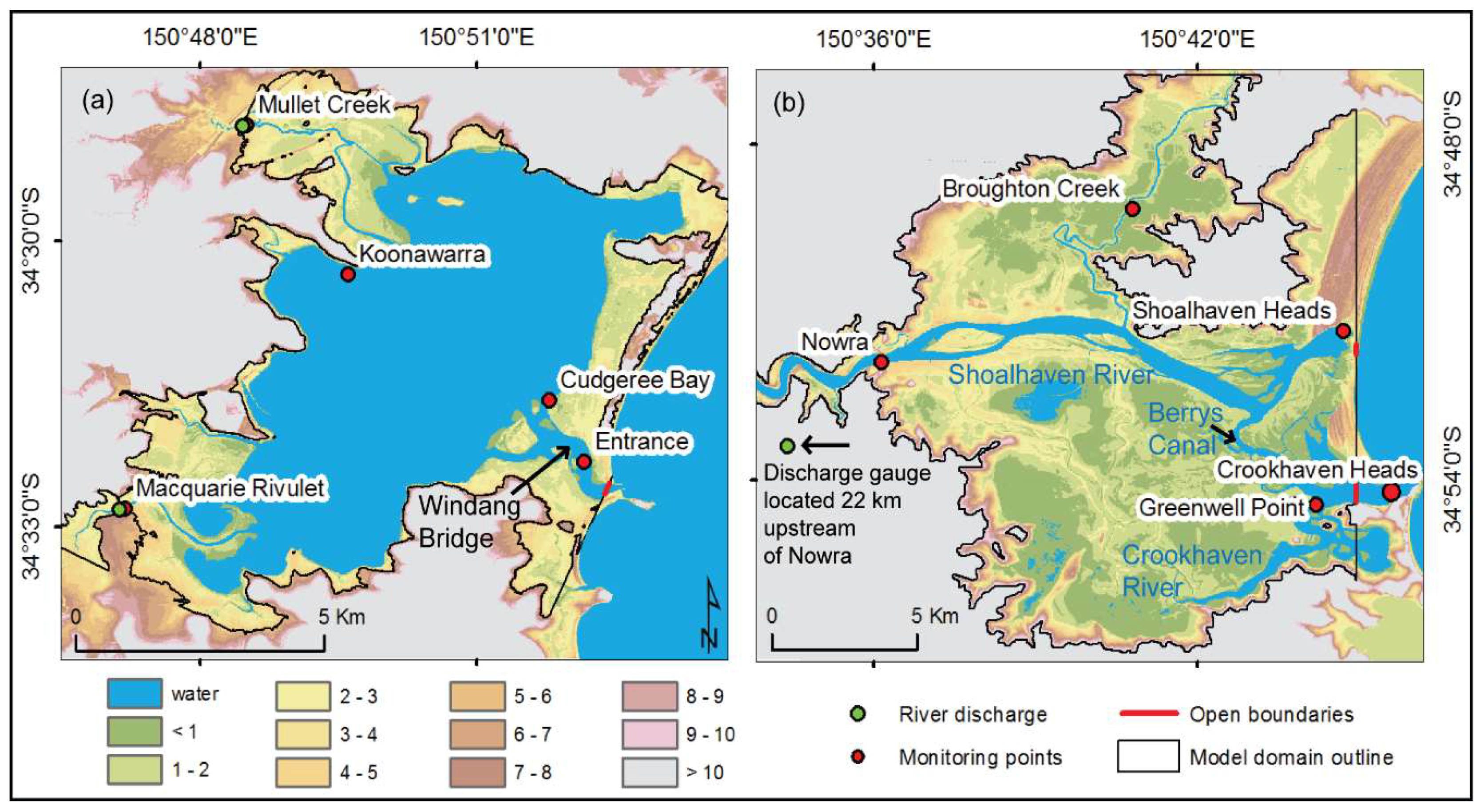
2. Study Sites
3. Materials and Methods
3.1. Input Data
3.2. Flood Drivers and SLR Scenarios
3.3. Hydrodynamic Modelling
4. Results
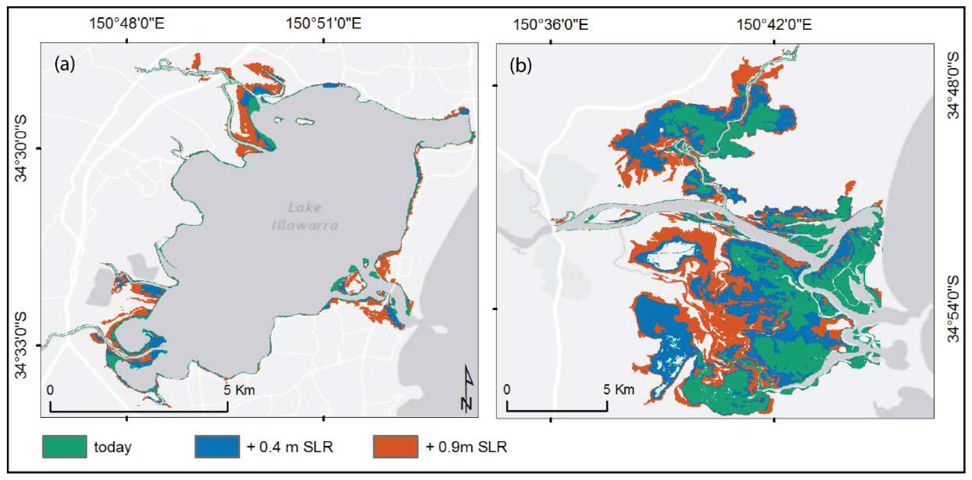
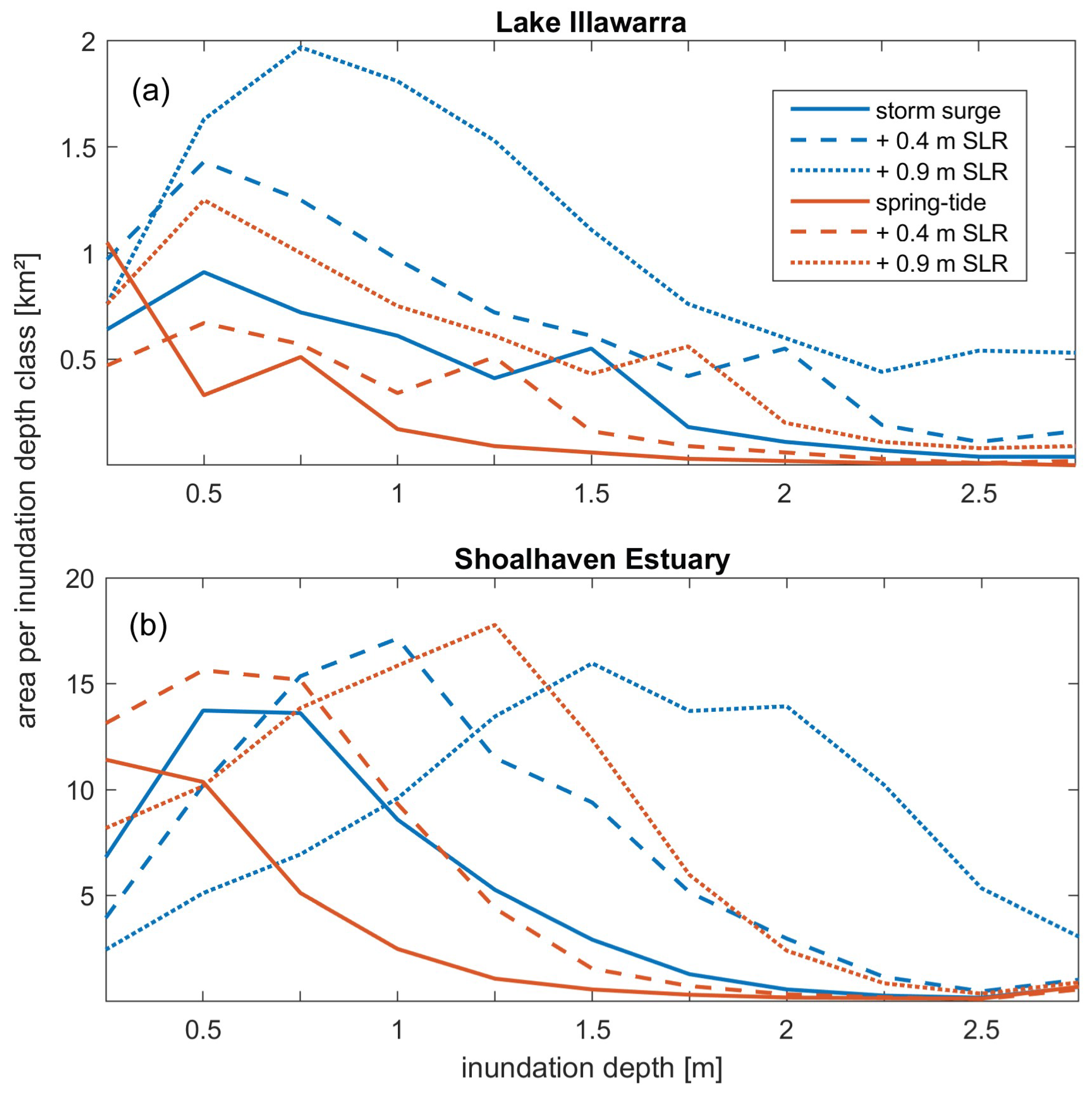
4.1. Inundation Extents and Depths
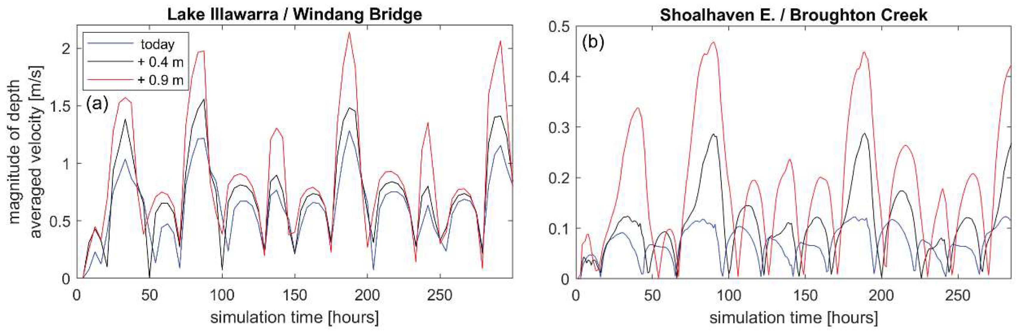
4.2. Hydrodynamics
5. Discussion
5.1. Changes in Inundation Extents and Depths
5.2. Hydrodynamic Response to SLR
6. Conclusions
Author Contributions
Acknowledgments
Conflicts of Interest
Appendix A

References
- Nicholls, R.J.; Wong, P.P.; Burkett, V.R.; Codignotto, J.O.; Hay, J.E.; McLean, R.F.; Ragoonaden, S.; Woodroffe, C.D. Coastal systems and low-lying areas. In Climate Change 2007: Impacts, Adaptation and Vulnerability. Contribution of Working Group II to the Fourth Assessment Report of the Intergovernmental Panel on Climate Change; Parry, M.L., Canziani, O.F., Palutikof, J.P., Van der Linden, P.J., Hanson, C.E., Eds.; Cambridge University Press: Cambridge, UK, 2007. [Google Scholar]
- Church, J.A.; Clark, P.U.; Cazenave, A.; Gregory, J.M.; Jevrejeva, S.; Levermann, A.; Merrifield, M.A.; Milne, G.A.; Nerem, R.S.; Nunn, P.D.; et al. Sea level change. In Climate Change 2013: The Physical Science Basis. Contribution of Working Group I to the Fifth Assessment Report of the Intergovernmental Panel on Climate Change; Stocker, T.F., Qin, D., Plattner, G.-K., Tignor, M., Allen, S.K., Boschung, J., Nauels, A., Xia, Y., Bex, V., Midgley, P.M., Eds.; Cambridge University Press: Cambridge, UK; New York, NY, USA, 2013. [Google Scholar]
- Dangendorf, S.; Marcos, M.; Wöppelmann, G.; Conrad, C.P.; Frederikse, T.; Riva, R. Reassessment of 20th century global mean sea level rise. Proc. Natl. Acad. Sci. USA 2017, 114, 5946–5951. [Google Scholar] [CrossRef] [PubMed]
- Nerem, R.S.; Beckley, B.D.; Fasullo, J.T.; Hamlington, B.D.; Masters, D.; Mitchum, G.T. Climate-change-driven accelerated sea-level rise detected in the altimeter era. Proc. Natl. Acad. Sci. USA 2018, 115, 2022–2025. [Google Scholar] [CrossRef] [PubMed]
- DeConto, R.M.; Pollard, D. Contribution of Antarctica to past and future sea-level rise. Nature 2016, 531, 591–597. [Google Scholar] [CrossRef] [PubMed]
- Oppenheimer, M.; Alley, R.B. How high will the seas rise? Science 2016, 354, 1375–1377. [Google Scholar] [CrossRef] [PubMed]
- McInnes, K.; Church, J.; Monselesan, D.; Hunter, J.; O’Grady, J.; Haigh, I.; Zhang, X. Information for Australian impact and adaptation planning in response to sea-level rise. Aust. Meteorol. Oceanogr. J. 2015, 65, 127–149. [Google Scholar] [CrossRef]
- Zhang, X.; Church, J.A.; Monselesan, D.; McInnes, K.L. Sea level projections for the Australian region in the 21st century. Geophys. Res. Lett. 2017, 44, 8481–8491. [Google Scholar] [CrossRef]
- Friedrichs, C.T.; Aubrey, D.G.; Speer, P.E. Impacts of Relative Sea-Level Rise on Evolution of Shallow Estuaries. Coast. Estuar. Stud. 1990, 38, 105–122. [Google Scholar]
- Nicholls, R.J.; Cazenave, A. Sea-level rise and its impact on coastal zones. Science 2010, 328, 1517–1520. [Google Scholar] [CrossRef] [PubMed]
- Geselbracht, L.L.; Freeman, K.; Birch, A.P.; Brenner, J.; Gordon, D.R. Modeled Sea Level Rise Impacts on Coastal Ecosystems at Six Major Estuaries on Florida’s Gulf Coast: Implications for Adaptation Planning. PLoS ONE 2015, 10, e0132079. [Google Scholar] [CrossRef] [PubMed]
- Lee, S.B.; Li, M.; Zhang, F. Impact of sea level rise on tidal range in Chesapeake and Delaware Bays. J. Geophys. Res. Oceans 2017, 122, 3917–3938. [Google Scholar] [CrossRef]
- Du, J.; Shen, J.; Zhang, Y.J.; Ye, F.; Liu, Z.; Wang, Z.; Wang, Y.P.; Yu, X.; Sisson, M.; Wang, H.V. Tidal Response to Sea-Level Rise in Different Types of Estuaries: The Importance of Length, Bathymetry, and Geometry. Geophys. Res. Lett. 2018, 45, 227–235. [Google Scholar] [CrossRef]
- Moftakhari, H.R.; AghaKouchak, A.; Sanders, B.F.; Matthew, R.A. Cumulative hazard: The case of nuisance flooding. Earth’s Future 2017, 5, 214–223. [Google Scholar] [CrossRef]
- Ikeuchi, H.; Hirabayashi, Y.; Yamazaki, D.; Muis, S.; Ward, P.J.; Winsemius, H.C.; Verlaan, M.; Kanae, S. Compound simulation of fluvial floods and storm surges in a global coupled river-coast flood model: Model development and its application to 2007 Cyclone Sidr in Bangladesh. J. Adv. Model. Earth Syst. 2017, 9, 1847–1862. [Google Scholar] [CrossRef]
- Olbert, A.; Comer, J.; Nash, S.; Hartnett, M. High-resolution multi-scale modelling of coastal flooding due to tides, storm surges and rivers inflows. A Cork City example. Coast. Eng. 2017, 121, 278–296. [Google Scholar] [CrossRef]
- Kumbier, K.; Carvalho, R.C.; Vafeidis, A.T.; Woodroffe, C.D. Investigating compound flooding in an estuary using hydrodynamic modelling: A case study from the Shoalhaven River, Australia. Nat. Hazards Earth Syst. Sci. 2018, 18, 463–477. [Google Scholar] [CrossRef]
- Kumbier, K.; Carvalho, R.C.; Vafeidis, A.T.; Woodroffe, C.D. Comparing static and dynamic flood models in estuarine environments: A case study from southeast Australia. Estuar. Coast. Shelf Sci. 2018. submitted. [Google Scholar]
- Poulter, B.; Halpin, P.N. Raster modeling of coastal flooding from sea level rise. Int. J. Geogr. Inf. Sci. 2008, 22, 167–182. [Google Scholar] [CrossRef]
- Van de Sande, B.; Lansen, J.; Hoyng, C. Sensitivity of coastal flood risk assessments to digital elevation models. Water 2012, 4, 568–579. [Google Scholar] [CrossRef]
- Passeri, D.L.; Hagen, S.C.; Medeiros, S.C.; Bilskie, M.V.; Alizad, K.; Wang, D. The dynamic effects of sea level rise on low-gradient coastal landscapes: A review. Earth’s Future 2015, 3, 159–181. [Google Scholar] [CrossRef]
- Watterson, E.K.; Burston, J.M.; Stevens, H.; Messiter, D.J. The hydraulic and morphological response of a large coastal lake to rising sea levels. In Proceedings of the 19th NSW Coastal Conference, Batemans Bay, Australia, 10–12 November 2010. [Google Scholar]
- Prandle, D.; Lane, A. Sensitivity of estuaries to sea level rise: Vulnerability indices. Estuar. Coast. Shelf Sci. 2015, 160, 60–68. [Google Scholar] [CrossRef]
- Yang, Z.; Wang, T.; Voisin, N.; Copping, A. Estuarine response to river flow and sea-level rise under future climate change and human development. Estuar. Coast. Shelf Sci. 2015, 156, 19–30. [Google Scholar] [CrossRef]
- Roy, P.S.; Williams, R.J.; Jones, A.R.; Yassini, I.; Gibbs, P.J.; Coates, B.; West, R.J.; Scanes, P.R.; Hudson, J.P.; Nichol, S. Structure and function of south-east Australian estuaries. Estuar. Coast. Shelf Sci. 2001, 53, 351–384. [Google Scholar] [CrossRef]
- Rogers, K.; Woodroffe, C.D. Geomorphology as an indicator of the biophysical vulnerability of estuaries to coastal and flood hazards in a changing climate. J. Coast. Conserv. 2016, 20, 127–144. [Google Scholar] [CrossRef]
- Thom, B. Coastal Geomorphology in Australia; Academic Press: Sydney, Australia, 1984; ISBN 0126878803. [Google Scholar]
- Short, A.D.; Woodroffe, C.D. The Coast of Australia; Cambridge University Press: Melbourne, Australia, 2009; ISBN 0521873983. [Google Scholar]
- Woodroffe, C.D.; Buman, M.; Kawase, K.; Umitsu, M. Estuarine infill and formation of deltaic plains, Shoalhaven River. Wetlands 2000, 18, 72–84. [Google Scholar]
- MHL NSW Tidal Planes Analysis 1990–2010 Harmonic Analysis, Report MHL2053. Available online: http://new.mhl.nsw.gov.au/docs/oeh/tidalplanes/mhl2053%20OEH%20tidal%20planes%20analysis%20final%20report.pdf (accessed on 10 October 2017).
- Hinwood, J.; McLean, E.; Trevethan, M. Spring Tidal Pumping. In Proceedings of the Coasts and Ports, Coastal Living-Living Coast: Australasian Conference, Adelaide, Australia, 20–23 September 2005. [Google Scholar]
- Carvalho, R.C.; Woodroffe, C.D. Rainfall variability in the Shoalhaven River catchment and its relation to climatic indices. Water Resour. Manag. 2015, 29, 4963–4976. [Google Scholar] [CrossRef]
- Webb, L.B.; Hennessy, K. Projections for Selected Australian Cities. Available online: https://www.climatechangeinaustralia.gov.au/media/ccia/2.1.6/cms_page_media/176/CCIA_Australian_cities_1.pdf (accessed on 14 September 2017).
- Burston, J.; Taylor, D.; Garber, S. Contextualizing the return period of the June 2016 East Coast Low: Waves, water levels and erosion. In Proceedings of the 25th NSW Coastal Conference, Coffs Harbour, Australia, 9–11 November 2016. [Google Scholar]
- Codiga, D.L. Unified Tidal Analysis and Prediction Using the UTide Matlab Functions, Technical Report 2011-01. Available online: http://www.po.gso.uri.edu/pub/downloads/codiga/pubs/2011Codiga-UTide-report.Pdf (accessed on 20 October 2016).
- Deltares. Delft3D-Flow. Simulation of Multi-Dimensional Hydrodynamic Flows and Transport Phenomena, Including Sediments, User Manual. Available online: https://oss.deltares.nl/documents/183920/185723/Delft3D-FLOW_User_Manual.pdf (accessed on 4 October 2016).
- Chow, V.T. Open Channel Hydraulics; Blackburn Press: New York, NY, USA, 1959; ISBN 1932846182. [Google Scholar]
- Fisher, K.; Dawson, H. Reducing Uncertainty in River Flood Conveyance, Roughness Review; DE-FRA/Environmental Agency Flood and Coastal Defense R&D Program: Lincoln, UK, 2003. [Google Scholar]
- Kaiser, G.; Scheele, L.; Kortenhaus, A.; Loevholt, F.; Roemer, H.; Leschka, S. The influence of land cover roughness on the results of high resolution tsunami inundation modelling. Nat. Hazards Earth Syst. Sci. 2011, 11, 2521–2540. [Google Scholar] [CrossRef]
- Woodroffe, C.D. Mangrove response to sea level rise: Palaeoecological insights from macrotidal systems in northern Australia. Mar. Freshwater Res. 2018, 69, 917–932. [Google Scholar] [CrossRef]
- Phan, L.K.; van Thiel de Vries, J.S.M.; Stive, M.J.F. Coastal mangrove squeeze in the Mekong Delta. J. Coast. Res. 2015, 31, 233–243. [Google Scholar] [CrossRef]
- Woodroffe, C.D.; Rogers, K.; McKee, K.L.; Lovelock, C.E.; Mendelssohn, I.A.; Saintilan, N. Mangrove Sedimentation and Response to Relative Sea-Level Rise. Annu. Rev. Mar. Sci. 2016, 8, 243–266. [Google Scholar] [CrossRef] [PubMed]
- Temmerman, S.; Meire, P.; Bouma, T.J.; Herman, P.M.J.; Ysebaert, T.; De Vriend, H.J. Ecosystem-based coastal defence in the face of global change. Nature 2013, 504, 79–83. [Google Scholar] [CrossRef] [PubMed]
- Van Coppenolle, R.; Schwarz, C.; Temmerman, S. Contribution of Mangroves and Salt Marshes to Nature-Based Mitigation of Coastal Flood Risks in Major Deltas of the World. Estuaries Coasts 2018, 13. [Google Scholar] [CrossRef]
- Bilskie, M.V.; Hagen, S.C.; Medeiros, S.C.; Passeri, D.L. Dynamics of sea level rise and coastal flooding on a changing landscape. Geophys. Res. Lett. 2014, 41, 927–934. [Google Scholar] [CrossRef]
- Wiecek, D.; Regena, C.; Laine, R.; Williams, R.J. Quantifying change and impacts to Lake Illawarra from a permanent opening. In Proceedings of the 25th NSW Coastal Conference, Coffs Harbour, Australia, 9–11 November 2016. [Google Scholar]
- Couriel, E.; Young, S.; Jayewardene, I.; McPherson, B.; Dooley, B. Case study: Assessment of the entrance stability of the Lake Illawarra Estuary. In Proceedings of the Coast and Ports 2013: Australasian Port and Harbour Conference Coasts and Ports 2013: 21st Australasian Coastal and Ocean Engineering Conference and the 14th Australasian Port and Harbour Conference, Sydney, Australia, 11–13 September 2013. [Google Scholar]
- Hanslow, D.; Morris, B.D.; Foulsham, E.; Kinsela, M.D. A regional scale approach to assessing current and potential future exposure to tidal inundation in different types of estuaries. Sci. Rep. 2018, 8, 1–13. [Google Scholar] [CrossRef] [PubMed]
- Mudersbach, C.; Wahl, T.; Haigh, I.D.; Jensen, J. Trends in high sea levels of German North Sea gauges compared to regional mean sea level changes. Cont. Shelf Res. 2013, 65, 111–120. [Google Scholar] [CrossRef]
- Idier, D.; Paris, F.; Le Cozannet, G.; Boulahya, F.; Dumas, F. Sea-level rise impacts on the tides of the European Shelf. Cont. Shelf Res. 2017, 137, 56–71. [Google Scholar] [CrossRef]
- Pickering, M.D.; Horsburgh, K.J.; Blundell, J.R.; Hirschi, J.J.M.; Nicholls, R.J.; Verlaan, M.; Wells, N.C. The impact of future sea-level rise on the global tides. Cont. Shelf Res. 2017, 142, 50–68. [Google Scholar] [CrossRef]


| Lake Illawarra | Shoalhaven Estuary | ||||
|---|---|---|---|---|---|
| Tide Gauge | r2 | rmse (m) | Tide Gauge | r2 | rmse (m) |
| Entrance | 0.97 | 0.12 | Greenwell Point | 0.98 | 0.09 |
| Cudgegree Bay | 0.98 | 0.12 | Shoalhaven Heads | 0.98 | 0.15 |
| Koonawarra | 0.97 | 0.14 | Nowra | 0.99 | 0.18 |
| Macquarie R. | 0.94 | 0.21 | |||
| Study Site and Flood Driver | Present | +0.4 m SLR | +0.9 m SLR | |||
|---|---|---|---|---|---|---|
| Inundation Extent (km2) | Average Inundation Depth (m) | Inundation Extent (km2) | Average Inundation Depth (m) | Inundation Extent (km2) | Average Inundation Depth (m) | |
| L. Illawarra | ||||||
| tide | 1.5 | 0.4 | 2.9 | 0.7 | 5.8 | 0.9 |
| storm-tide | 4.3 | 0.8 | 7.3 | 0.9 | 11.6 | 1.1 |
| compound | 5.1 | 0.8 | 8.1 | 0.9 | 12.1 | 1.1 |
| Shoalhaven | ||||||
| tide | 32 | 0.5 | 62 | 0.6 | 89 | 0.9 |
| storm-tide | 54 | 0.7 | 78 | 1.0 | 100 | 1.4 |
| compound | 75 | 0.8 | 91 | 1.1 | 104 | 1.6 |
© 2018 by the authors. Licensee MDPI, Basel, Switzerland. This article is an open access article distributed under the terms and conditions of the Creative Commons Attribution (CC BY) license (http://creativecommons.org/licenses/by/4.0/).
Share and Cite
Kumbier, K.; Carvalho, R.C.; Woodroffe, C.D. Modelling Hydrodynamic Impacts of Sea-Level Rise on Wave-Dominated Australian Estuaries with Differing Geomorphology. J. Mar. Sci. Eng. 2018, 6, 66. https://doi.org/10.3390/jmse6020066
Kumbier K, Carvalho RC, Woodroffe CD. Modelling Hydrodynamic Impacts of Sea-Level Rise on Wave-Dominated Australian Estuaries with Differing Geomorphology. Journal of Marine Science and Engineering. 2018; 6(2):66. https://doi.org/10.3390/jmse6020066
Chicago/Turabian StyleKumbier, Kristian, Rafael C. Carvalho, and Colin D. Woodroffe. 2018. "Modelling Hydrodynamic Impacts of Sea-Level Rise on Wave-Dominated Australian Estuaries with Differing Geomorphology" Journal of Marine Science and Engineering 6, no. 2: 66. https://doi.org/10.3390/jmse6020066
APA StyleKumbier, K., Carvalho, R. C., & Woodroffe, C. D. (2018). Modelling Hydrodynamic Impacts of Sea-Level Rise on Wave-Dominated Australian Estuaries with Differing Geomorphology. Journal of Marine Science and Engineering, 6(2), 66. https://doi.org/10.3390/jmse6020066