Seeing Through the Waste: MD-YOLO for Precise Localization of Marine Debris

Abstract

Marine ecosystem integrity is paramount to global stability. With the advancement of industrialization, various types of waste are discharged into the ocean, accumulating through the food chain and ultimately threatening human health and the global climate environment. To achieve precise and efficient cleanup of marine debris, traceability is essential, with detection and classification serving as critical steps. To address the issues of missed detection and occlusion caused by the irregular shapes of marine debris due to water pressure or structural characteristics, as well as the coexistence of multi-scale objects resulting from aggregation and shooting angles, this study proposes the MD-YOLO model based on the YOLOv11L architecture. Firstly, a deformable attention mechanism is introduced in the neck network to achieve dynamic sampling and precise localization of targets with imbalanced aspect ratios. Secondly, a context-aware multi-scale feature fusion module is embedded in the backbone network to effectively mitigate the issue of missed detection of small targets when objects of different sizes coexist. Finally, a cooperative spatial-channel attention mechanism is designed in the detection head to enhance the feature representation capability in visible regions and infer occluded areas, thereby significantly suppressing occlusion interference. Experiments conducted on a self-constructed dataset containing 5095 images demonstrate that the proposed method achieves 86.7% in mAP@0.5, 67.6% in mAP@0.5:0.95, and an F1 score of 0.83, significantly outperforming comparative methods. This study provides key technical support for the effective traceability of marine debris.

1. Introduction

As a vital component of Earth’s ecosystem, the health of the ocean directly impacts global climate regulation, biodiversity conservation, and sustainable human development [1]. However, with global population growth, accelerated industrialization, and widespread plastic use, various waste materials are continuously entering the ocean through rivers, sewage discharge, shipping activities, and coastal operations, forming massive marine debris [2]. According to a United Nations Environment Programme report, over 8 million tons of plastic waste enter the ocean annually, with total quantities reaching hundreds of millions of tons [3]. These wastes, particularly non-biodegradable plastics, can persist in the ocean for centuries [4]. They not only directly cause the death of seabirds, fish, and marine mammals due to entanglement or ingestion, but also form “plastic rings” through physical friction, chemical leaching, and pollutant adsorption [5].

The rapid advancement of object detection algorithms has provided robust technical support for marine debris identification. In the detection of targets with non-standard aspect ratios, Ren et al. proposed the Faster R-CNN framework. By generating candidate bounding boxes through Region Proposal Network (RPN) and predefining multi-scale anchor boxes, combined with Region of Interest (RoI) pooling for feature processing, this approach significantly enhances adaptability to diverse geometric targets [6]. Law et al. introduced the anchorless detection algorithm CornerNet, which detects target corners (top-left and bottom-right) and matches embedded vectors to form bounding boxes, reducing computational overhead and proving particularly effective for detecting objects with abnormal aspect ratios [7]. Zhou et al. developed ExtremeNet, extending keypoint detection to four extreme points (top, bottom, left, and right) [8]. By calculating geometric centers and querying center point heatmaps to combine bounding boxes, this method reduces embedded learning costs while improving detection accuracy. Tian et al. proposed the fully convolutional single-stage detector FCOS, which introduces centrality branches to quantify the correlation between predicted positions and target centers, suppressing low-quality predictions to enhance recall accuracy and bounding box localization quality [9]. Ge et al. abandoned predefined anchor boxes, adopting a center point prediction mechanism and separating classification from regression tasks [10]. By adapting to target size and density via dynamic allocation, this method greatly enhances detection of objects with abnormal aspect ratios.

In response to the diverse sizes of marine debris, researchers have proposed tailored solutions based on specific practical scenarios. Lin et al. proposed the Feature Pyramid Network (FPN), which constructs multi-scale feature pyramids to effectively reduce information loss during downsampling, thereby enhancing the model’s multi-scale processing capability with minimal computational cost [11]. Liu et al. introduced the Single-Scale Detection (SSD) method, performing detection directly on multi-scale feature maps while using predefined multi-scale prior bounding boxes as positional references, significantly reducing regression challenges in localization tasks [12]. Tan et al. developed EfficientDet, employing a weighted bidirectional pyramid network (BiFPN) for efficient multi-scale feature fusion and a composite scaling strategy to coordinate network expansion across dimensions, achieving higher precision with fewer parameters and computation [13]. Zhou et al. proposed the Multi-Scale Target Detector (MSSD), utilizing spatial pyramid deep convolution to enhance perceptual fields and integrating multi-scale features through channel attention mechanisms, improving detection performance without compromising real-time processing [14]. Zhao et al. innovatively introduced hybrid encoders that decouple intra-scale interactions and cross-scale fusion to capture multi-scale features, enhancing the model’s ability to process objects of varying scales while maintaining real-time performance [15].

In the field of object detection under occlusion, occlusion is a primary cause of incomplete target features and detection failures, particularly prevalent in densely accumulated marine debris. Zhou et al. proposed an anti-occlusion method based on the Kernel Correlation Filtering (KCF) framework, which dynamically updates filter templates by combining response difference changes and gradient variations to improve localization accuracy under occlusion [16]. Gong et al. introduced Kalman filtering for motion prediction in YOLOv3 and designed a hierarchical data association mechanism, performing secondary matching of occluded targets through appearance similarity to effectively reduce occlusion interference [17]. Wang et al. proposed the Programmable Gradient Information (PGI) concept, generating reliable gradients via auxiliary reversible branches to reduce semantic loss in deep supervision [18]. They designed a generalized efficient layer aggregation network, replacing conventional convolutions in the original efficient layer aggregation network with Cross Stage Partial (CSP) modules [19], and improved the first-layer convolutions of CSP bottleneck modules using reparametrized convolutional structures to enhance feature extraction capabilities [20]. Zhou et al. proposed an occlusion-based object detection model based on improved YOLOv8 [21,22], dynamically adjusting convolution kernel parameters through Adaptive Kernel Convolution (AKConv) fusion to achieve more accurate detection in occluded environments [23]. Fan et al. employed the Sinkhorn-Knopp iterative method to simplify optimal transport allocation (OTA), enabling more rational sample distribution in occluded scenes from a global perspective and enhancing the model’s detection performance for occluded targets [24].

A variety of algorithms have been deployed in real-world marine environments. In foundational early work, Valdenegro-Toro pioneered the technical feasibility of deep learning for detecting submerged hidden debris by applying convolutional neural networks to forward-looking sonar imagery [25,26]. As target detection frameworks advanced, research priorities shifted toward enhancing models’ comprehensive performance in complex marine environments. Zhou et al. proposed YOLO TrashCan, which significantly improved detection accuracy in dim and turbid underwater environments through feature-enhancement modules [27]. Zocco et al. focused on edge computing scenarios, optimizing EfficientDet’s architecture and training strategies to achieve efficient real-time detection on mobile platforms like autonomous underwater vehicles (AUVs) [28]. To address complex background interference caused by waves and sun glint, researchers have utilized attention mechanisms to better focus on target regions. Meanwhile, they have leveraged the unique spectral features of hyperspectral images to distinguish plastic materials, while enhancing the clarity of physical interpretation. Confronting practical challenges such as widespread turbidity in coastal waters, varying target sizes, and diverse background complexities, scholars have modified mainstream detection models [29]. Yang et al. enhanced multi-scale representation capabilities by constructing a more refined feature pyramid or incorporating context-aware modules to capture targets at millimeter-to-meter scales [30]. Luo et al. and Pushkala et al. prioritized lightweight network designs, visual Transformers, or attention mechanisms to suppress background noise in complex sea conditions, thereby improving feature discrimination and anti-interference performance [31,32]. Gu et al. and Prabu et al. improved model training stability and generalization through optimized sample allocation and ensemble learning techniques [33].

In the expansion of monitoring capabilities and quantitative applications, Sasaki et al. and Booth et al. utilized high-resolution commercial satellite imagery and free mid-resolution satellite data; they developed density mapping and quantitative assessment methods for floating debris in coastal zones and open seas, achieving a breakthrough from discrete target recognition to continuous spatial distribution analysis [34]. These methods provide critical tools for evaluating regional pollution loads and identifying cross-border transport hotspots [35]. Bergui et al. released the MADLib hyperspectral reference database, systematically collecting standardized spectral fingerprints of various marine debris which lays the groundwork for future development of spectral feature-based material classification [36].

This paper proposes an improved approach based on the YOLOv11 model. The core idea is to develop a collaborative enhancement scheme centered on the attention mechanism, systematically strengthening three key aspects: feature sampling, feature fusion, and feature purification. This enables the model to adaptively handle geometric distortions, scale variations, and occlusion interference. The main contributions are as follows:

(1)

Integrating deformable attention mechanism into the neck network of the model. This mechanism enables the network to dynamically adjust the sampling point positions based on target semantics, rather than relying on fixed grids.

(2)

Construct a multi-scale feature extraction module. This module employs multi-branch convolution to extract features and achieves adaptive, selective multi-scale information fusion by learning the importance weights of feature channels at different scales.

(3)

We design a collaborative spatial-channel dual-attention unit. This unit focuses on the target’s visible effective region in spatial dimension while enhancing key semantic features critical for category discrimination in channel dimension.

This study validates the effectiveness of the proposed method on real-world scenario datasets, providing a novel solution for constructing a high-precision, robust, and practical intelligent marine debris detection system.

The remainder of this paper is organized as follows: Section 2 elaborates the self-constructed marine debris dataset, including data acquisition, cleaning and preprocessing, annotation protocols, as well as data statistics and visualization analysis. Section 3 introduces the baseline YOLOv11L network architecture and the proposed MD-YOLO framework, detailing the designed deformable attention-based dynamic sampling, context-aware multi-scale feature extraction, and collaborative spatial-channel attention module for occlusion disturbance processing. Section 4 provides experimental configuration and comprehensive performance analysis, covering ablation experiments, comparative experiments with mainstream detectors, and visualization results. Finally, Section 5 concludes the paper and discusses future research directions including architecture-efficiency co-optimization and spatio-temporal-3D perception.

2. Datasets

2.1. Data Acquisition

The marine debris dataset in this study comprises images from three distinct sources. The first is the Institutional Collaborative Marine Debris Dataset, which features exceptionally high-quality images with precise annotations, providing reliable supervised data for model training [37]. The second is the Institutional Satellite and UAV Marine Debris Dataset, containing rich environmental details that enhance the model’s recognition robustness in specific scenarios. The third is the Web-collected Marine Debris Image Dataset [38], characterized by varying resolutions, diverse shooting angles, frequent perspective distortions, obstructions, and cluttered backgrounds.

2.2. Data Cleaning and Preprocessing

To ensure data quality, this section performed cleaning on the collected raw marine debris images [39] to remove damaged files. The cleaning process was completed in a Python environment and primarily included three stages: file integrity check, data deduplication, and pixel quality assessment.

File integrity checks verify the ability to read files correctly, ensuring they remain undamaged during storage or transmission [40].

After removing incomplete images, further deduplication is required to ensure image data diversity. The deduplicate_images method is implemented based on the concept of unique hash values for each image, utilizing the mean hashing algorithm to compute perceptual hashes [41]. The calculate_perceptual_hash(image_path) function first normalizes images through cubic spline interpolation, compressing them to 8 × 8 resolution. Color images are then converted to grayscale using the grayscale value calculation Formula (1). The arithmetic mean of all grayscale pixels is computed using the mean calculation Formula (2). Hash bits are generated according to the judgment rule (3), and serialized hashes are created in lexicographic order. Each image’s hash value is recorded and compared, with duplicates being quickly removed to achieve image deduplication.

$$\mathrm{G}\mathrm{r}\mathrm{a}\mathrm{y}=\sqrt[32]{R^{22}\times 0.2973+G^{22}\times 0.6274+B^{22}\times 0.0753}.$$

(1)

Gray is the calculated grayscale value. $R$, $G$, $B$ represent the pixel values of the red, green, and blue channels of the input image, respectively. The coefficients are the standard weights for grayscale conversion.

Using the mean calculation formula shown in Equation (2), the arithmetic average of all pixel values in the grayscale image is computed.

$$\mu ={\displaystyle \frac{1}{64}}\sum _{i=1}^8\sum _{j=1}^{8}J(i,j).$$

(2)

μ denotes the arithmetic mean of all grayscale pixels. I(i, j) represents the pixel value at position (i, j) in the grayscale image.

Based on the calculated pixel mean, hash bits are generated following the decision rule shown in Equation (3), and a serialized hash is produced in row-major order. The hash value of each image is recorded and compared, quickly deleting images with identical hash values to achieve image deduplication.

$$h_{\mathbf{y}}=\left\{\begin{array}{l}1, \mathrm{i}\mathrm{f}\hspace{0.17em}I(i,j)>\mu ;\\ 0,\hspace{1em}\mathrm{o}\mathrm{t}\mathrm{h}\mathrm{e}\mathrm{r}\mathrm{w}\mathrm{i}\mathrm{s}\mathrm{e}.\end{array}\right.$$

(3)

$h_{\mathbf{y}}$ is a hash bit generated by comparing pixel values with the mean value $\mu$.

In pixel defect detection, the process is carried out in two aspects: noise detection and blur detection. Before the detection begins, the original image is first converted to grayscale using Equation (1).

The core idea of noise detection is local anomaly detection. In normal image regions, pixels have spatial continuity. Their values change gradually within a local neighborhood. In contrast, noisy pixels differ significantly from their neighbors, appearing as local outliers. For detection, a local statistical method is used. A 3 × 3 sliding window samples the image. The local variance of the grayscale image is calculated using Equation (4). This variance is then used to determine the proportion of noise.

$${Var}_C(x,y)={\displaystyle \frac{1}{9}}{\sum _{i=1}^1\sum _{j=1}^1\left(I(x+i,y+j)-{\displaystyle \frac{1}{9}}\sum _{i=1}^1\sum _{j=1}^{1}I(x+i,y+j)\right)}^2.$$

(4)

Var_c(x, y) represents the local variance of a grayscale image. I(x, y) denotes the pixel value of the grayscale image at position (x, y).

The loss of high-frequency information in images results in image blurring. This attenuation is caused by factors like optical defocus, motion blur, or noise [42]. In detection, the Laplace operator is introduced as a second-order differential operator. It is highly responsive to high-frequency image information, such as edges and details. The Laplace variance is calculated using Equation (5). A threshold of 100 is set for blur judgment: regions with a variance below this threshold are marked as blurred, while others are classified as clear.

$${Var}_L(l)={\displaystyle \frac{1}{MN}}{\sum _{i=0}^{M-1}\sum _{j=0}^{N-1}\left(\sum _{(m,n)\in \mathsf{\Gamma }}v(m,n)I(m+i,n+j)-{\displaystyle \frac{1}{MN}}\sum _{i=0}^{M-1}\sum _{j=0}^{N-1}I(m+i,n+j)\right)}^2.$$

(5)

Variable $I$ represents the input grayscale image, while $v(m,n)$ denotes the weight kernel of the Laplacian operator. $M$ and $N$ are the image dimensions. Γ is the neighborhood of the Laplacian operator.

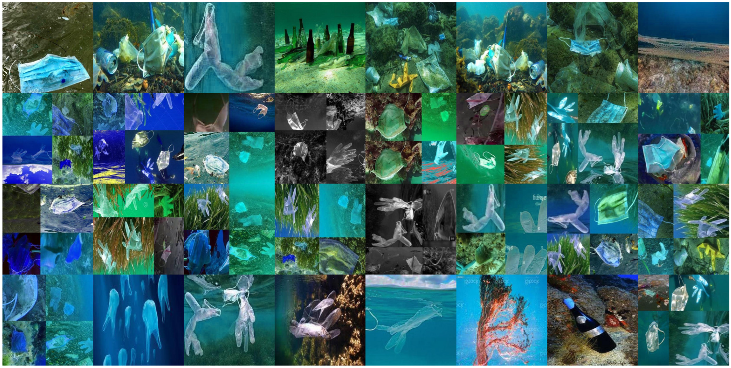
The image of marine garbage in the data set after data cleaning is shown in Figure 1.

The data sources, quantity, size, and categories in the dataset are shown in

Table 1. Statistics of the raw data sources for the Marine_Debris_detect dataset.

Data Source	Number of Original Images	Original Image Size	Classes Covered
Institutional Collaborative Marine Debris Dataset	376	1920 × 1080	All 8 classes
Institutional Satellite and UAV Marine Debris Dataset	1062	Varies (512 × 512 to 4000 × 3000)	Mask, Can, Gbottle, Glove, Misc, Net
Public Media and User-Generated Marine Debris Dataset	3889	Varies (640 × 480 to 3840 × 2160)	Mask, Can, Glove, Electronics, Misc, Net
Total (Before Deduplication)	5327	-	All 8 classes
After Deduplication (Final)	5095	-	All 8 classes

.

2.3. Data Annotation

In marine debris detection tasks, each marine debris image annotation must precisely include the following two key categories of information.

(1)

Target location information: Use rectangular bounding boxes to precisely outline all identifiable marine debris objects in the image. The bounding boxes should align with the edges of the debris objects while minimizing background inclusion.

Category information: Assign corresponding marine debris category labels to each annotation box, as specified in

Table 2. Label Annotation.

Category (Label Name)	Definition and Scope
Mask	Typically blue, white, or black, with prominent ear loops and pleated surfaces, which may appear spread or coiled in the ocean.
Can	Typically cylindrical in shape, the surface may bear printed patterns or labels and often exhibits deformation due to compression. The metallic surface features high-gloss reflective characteristics.
Electronics	It typically consists of various materials such as plastic and metal, may feature structures like buttons and interfaces.
Gbottle	Clear or colored, with well-defined contours, the bottle may have a raised trademark, and is prone to breaking into sharp fragments in the ocean.
Glove	It is usually hand-shaped, with five fingers distinguishable or in a lump-like form, and the material may appear semi-transparent or opaque.
Metal	Other metal fragments that cannot be classified as “Can” are irregular in shape, with sharp edges and a distinct metallic luster.
Net	The structure is in the form of a net, with the mesh size is different, often with the water plant entwined, or wrapped up other garbage, the form has the repeated linear texture and node.
Misc	All other human-made waste that cannot be classified into the above categories.

.

(2)

Table 2: Label annotation of the label annotation standard.

The annotation process utilizes the LabelImg annotation tool (version 1.8.0) for bounding box drawing and label tagging. The annotation results are stored in YOLO format as .txt files, with each file sharing the same name as its corresponding image and placed in the same directory structure for direct reading during model training.

The annotation follows a collaborative workflow involving dual annotators and a third-party arbitrator to resolve conflicts. Two annotators independently annotate the same batch of images without access to each other’s results. After annotation completion, the system first calculates the Intersection Over Union (IoU) ratio of object bounding boxes within the same image, identifying bounding boxes with IoU below 0.85 as conflicting matches. It then compares classification labels assigned by two annotators for the same object to detect semantic discrepancies. Finally, discrepancies are aggregated into a conflict set for third-party arbitration, ensuring consistency and reliability of annotation results.

To ensure a rigorous evaluation, the cleaned dataset of 5095 images was partitioned into training, validation, and test sets with a ratio of 72%:8%:20%, corresponding to 3626, 501, and 968 images, respectively.

Firstly, the split was performed using a stratified sampling method at the image level. This ensures that the distribution of categories is approximately proportional across all three splits, preventing significant class imbalance in any single subset.

Secondly, the perceptual hash-based deduplication process was applied to the entire dataset beforethe split. This guarantees that no duplicate or near-duplicate images can appear in different splits, effectively eliminating a common source of data leakage and ensuring that the test set represents truly unseen data.

Thirdly, the deduplication algorithm identified and removed 173 pairs of near-duplicate images. The final count of 5095 images represents the unique set used for all experiments. The effectiveness of this step is validated by the negligible hash collisions observed in the remaining dataset.

Finally, we did not apply explicit class re-weighting or resampling during training, as the baseline and proposed models were trained under identical conditions for fair comparison.

The divided dataset is named Marine_Debris_detect.

2.4. Data Statistics and Visualization Analysis

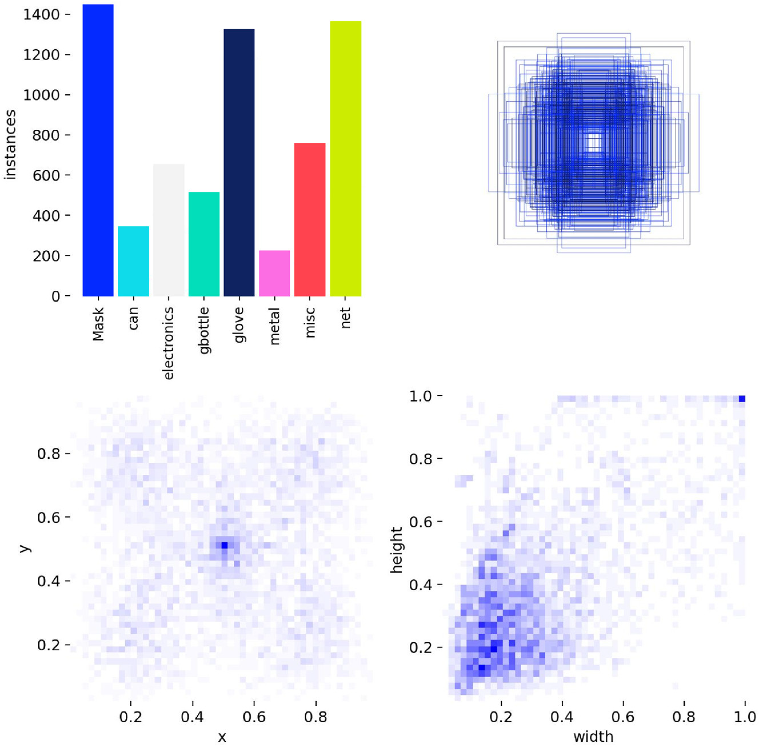
Figure 2 presents statistical analysis of the self-built dataset in this study. The bar chart in the upper left corner displays quantitative comparisons across eight categories, with instance counts as follows: Mask (1487), Can (342), Electronics (658), Gbottle (534), Glove (1356), Metal (211), Misc (787), and Net (1329). Analysis reveals Mask as the predominant category (22.18%) and Metal as the least represented (3.15%), clearly demonstrating significant category imbalance that accurately reflects real-world scenarios. Masks, gloves, and fishing nets are common pollutants in marine debris, confirming the dataset’s well-defined category classifications and substantial sample size. The bounding box overlap diagram in the upper right corner visually illustrates target scale diversity. The horizontal axis (X-axis) denotes the normalized width of bounding boxes, and the vertical axis (Y-axis) denotes the normalized height of bounding boxes, with both axes mapped to the range [0, 1] relative to the 640 × 640 input image size. This figure is obtained by calculating and normalizing the width and height of all annotated bounding boxes in the dataset, then plotting their joint distribution to show the overall scale and aspect ratio characteristics of marine debris objects.

The diagram covers both tiny objects and large-scale targets that occupy substantial image areas, demonstrating comprehensive coverage from micro-debris to macro-waste. The heat map showing target centroid distribution in the lower left corner reveals spatial patterns concentrated in mid-to-lower image regions with uniform horizontal distribution. This non-random distribution pattern reflects realistic scene constraints and aligns with practical application scenarios. The bounding box width–height distribution scatterplot in the lower right corner illustrates size relationships between object dimensions, showing most targets clustered in small-size regions while including numerous medium-to-large targets, demonstrating multi-scale coexistence. The point cloud analysis reveals no significant outliers or single clusters, confirming diverse object shapes and sizes.

As presented in

Table 3. Statistics of the eight marine debris categories in the Marine_Debris_detect dataset.

Class Name	Number of Instances (Bounding Boxes)	Percentage (%)	Number of Images Containing the Class
Mask	1487	22.18	326
Can	342	5.1	114
Electronics	658	9.82	196
Gbottle	534	7.96	163
Glove	1356	20.23	301
Metal	211	3.15	79
Misc	787	11.74	242
Net	1329	19.83	298
Total	6694	100	5095

, statistics of the eight marine debris categories in the Marine_Debris_detect dataset, complete and consistent statistical details are provided for all eight marine debris categories. For each class, we list the total number of annotated instances (bounding boxes), its percentage proportion in the dataset, and the number of independent images that contain at least one object of this class. The statistics reveal a natural class imbalance in real-world marine environments, which is in line with the actual distribution of marine debris.

3. Proposed MD-YOLO Method

3.1. YOLOv11L Network Architecture

In this study, we selected YOLOv11, which has both accuracy and speed, as the benchmark architecture. It offers five model sizes—n, s, m, l, and x. Considering that the marine debris localization task in this study requires balancing detection accuracy and computational efficiency in complex marine scenes, the l-sized model provides the optimal equilibrium between performance and resource consumption. Therefore, this research adopts YOLOv11L as the baseline model.

The proposed C3k2 module in YOLOv11L processes information using C3K blocks [43]. It optimizes the information flow in the network by splitting feature maps and applying a series of smaller 3 × 3 kernel convolutions. By handling smaller, independent feature maps and merging them after several convolutions, it operates faster and with lower computational cost compared to the C2F module in YOLOv8.

The C2PSA module used in YOLOv11L introduces an attention mechanism. By emphasizing spatial correlations in feature maps, it applies spatial attention to the extracted features, refining the model’s ability to selectively focus on regions of interest. This enhances the model’s attention to important areas in the image.

YOLOv11L employs a multi-scale prediction head to detect objects of varying sizes. The head uses feature maps generated by the backbone and neck networks to output detection boxes at three different scales: low (P3 layer), medium (P4 layer), and high (P5 layer). The detection head makes predictions based on the three acquired feature maps, corresponding to different granularity levels in the image. This approach ensures that smaller objects are detected with finer detail, while larger objects are captured by higher-level features.

3.2. The MD-YOLO Framework

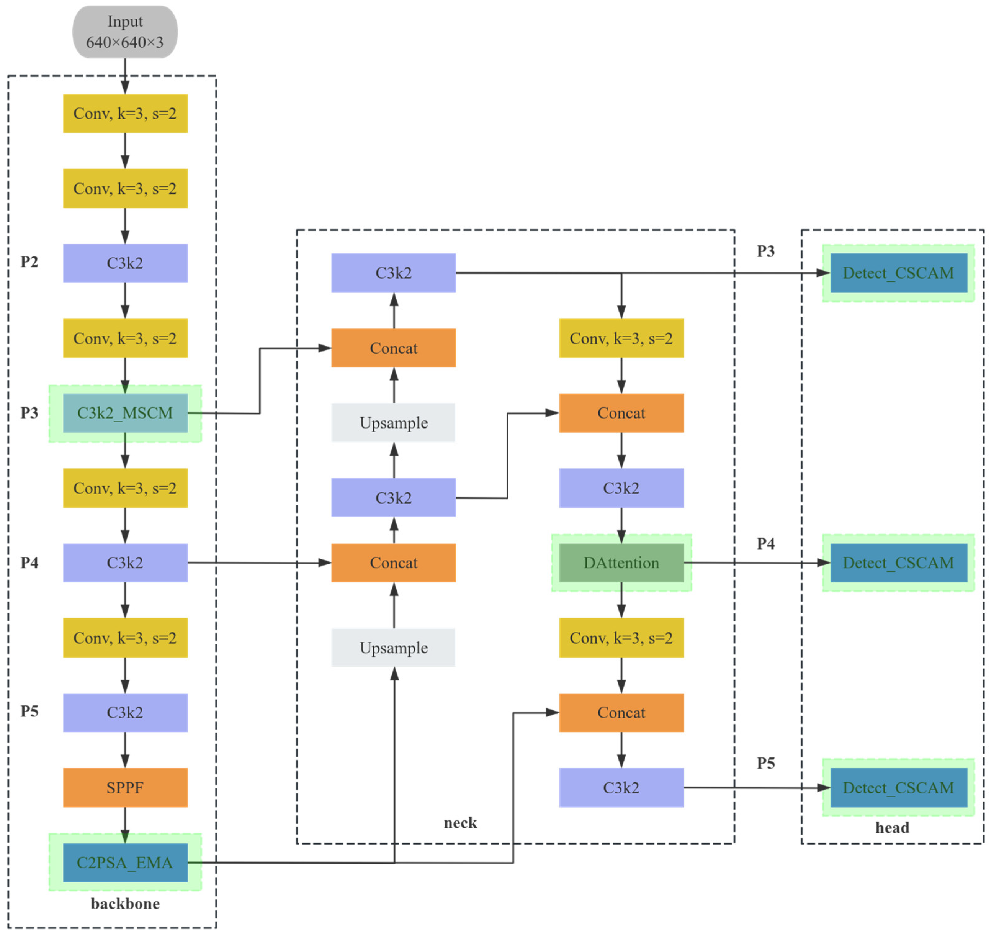
We propose MD-YOLO—an enhanced version of YOLOv11L. Its network structure is illustrated in Figure 3. This new model significantly improves marine debris detection accuracy while maintaining real-time performance. The architectural enhancements include the following optimizations.

Firstly, a deformable attention mechanism is incorporated into the neck network. By leveraging dynamic sampling, it enables the model to adaptively adjust the receptive field and focus on sparse key features of targets with abnormal aspect ratios, effectively suppressing background interference.

Secondly, building on the concept of multi-scale feature extraction, a multi-scale convolutional module and an efficient multi-scale attention mechanism are embedded into the backbone network. Through the design of multi-branch parallel convolutions and cross-scale feature re-weighting, the model’s ability to capture features of large, medium, and small-sized marine debris coexisting in scenes is enhanced, significantly reducing missed detections.

Finally, a cooperative spatial-channel attention mechanism is designed in the detection head. By integrating spatial confidence evaluation and channel importance re-weighting, it strengthens the features of visible parts of occluded targets, suppresses interference from occluding objects, and improves localization accuracy in occlusion scenarios.

3.3. Dynamic Sampling Based on Deformable Attention

In complex marine environments, target debris often exhibits significant length-to-width disparities in images due to factors like camera angles or varying debris shapes. This imbalanced aspect ratio causes the effective features of the marine debris target on the feature map to be sparsely and elongated.

In YOLOv11L, the neck network bridges the backbone and detection head, performing multi-scale feature fusion and information enhancement. It integrates feature maps from different levels output by the backbone network, preserving local information from large-scale feature maps while extracting high-level semantic content from small-scale feature maps. It then concatenates and fuses low-level details with high-level semantics, enriches contextual representation, and finally processes them further through convolution and attention mechanisms before passing them to the detection head to complete the detection and localization tasks.

During the feature processing pipeline in the neck network, traditional self-attention mechanisms typically rely on a fixed-range receptive field, adjusting feature responses through weight allocation within a global or local scope.

Let the input feature map be denoted as $F\in {\mathbb{R}}^{C\times H\times W}$. The response of the traditional attention mechanism at a query position q can be expressed as:

$$y_q=\sum _{k\le \Omega }A(q,k)E_k,$$

(6)

$y_q$ denotes the response at query position $q$. Ω represents the fixed sampling neighborhood. A(q, k) indicates the attention weight. E_k denotes the feature of the key.

This mechanism performs well in general object detection. It is stable, efficient, and captures context effectively. However, real-world marine debris is different from standard natural images. Debris often exhibits extreme aspect ratios due to varying camera angles and intrinsic object geometry. Traditional self-attention mechanisms, constrained by fixed receptive fields, fail to adapt to these irregular boundaries. Consequently, they inadvertently incorporate irrelevant background or occluded features, leading to noise accumulation, feature contamination, and compromised localization accuracy.

To address this, we propose an improved Deformable Attention mechanism (DAT). Unlike standard attention, DAT predicts offsets for each query point to dynamically shift sampling locations. This allows the model to align with irregular object geometries, effectively filtering out background noise and significantly improving bounding box accuracy for marine debris.

Within this deformable attention mechanism, group convolution is first utilized to partition the feature channels, reducing resource consumption. Subsequently, during the computation for offset generation, considering the characteristic of imbalanced aspect ratios in marine debris images, Batch Normalization (BatchNorm)—which normalizes the same feature across different samples—is abandoned. Instead, Layer Normalization (LayerNorm), which computes the mean and variance for different features within a single sample, is chosen. This enables sample-specific feature processing. Meanwhile, the GeLU activation function is introduced to achieve nonlinear enhancement, generating the final offsets $\Delta p$. The obtained offsets $\Delta p$ are then applied to the original reference points p to derive new deformed points, ultimately forming new deformed positions. Finally, based on the dynamic sampling positions, bilinear interpolation is performed to obtain the sampled features, and a projection matrix is used to generate weights for weighted summation on the feature map:

$$y_q=\sum _{m=1}^M{A}_m(q)\cdot F\left(q+\Delta p_q^m\right).$$

(7)

Here, $M$ represents the sampling point positions, $\Delta p_q^m$ is predicted by the network and adaptively associated with the target morphology, and $A_m\left(q\right)$ denotes the attention weights corresponding to the sampling points.

3.4. Context-Aware Multi-Scale Feature Extraction

The original YOLOv11L model struggles with the challenge of significant scale variations in marine debris images due to its fixed-size convolutional kernels. Its single receptive field fails to fully capture the global structure of large debris objects and tends to lose small target details during feature transfer, resulting in missed detections and ultimately compromising overall detection performance.

To address the aforementioned challenges, this section adopts the core concept of multi-scale feature fusion to make targeted improvements to the feature extraction network. We construct a hierarchical feature representation that unifies local details with global semantics. By integrating multi-branch convolutions and multi-scale attention reweighting, our approach aggregates cross-layer information, effectively bridging the gap between fine-grained textures and high-level context.

In CNNs, the receptive field—dictated by kernel size—governs the spatial scope of feature capture. Small-scale kernels (1 × 1 size) are commonly used to enable cross-channel information exchange and integration, focusing on extremely local features. Medium-scale kernels (3 × 3 size) represent the most typical and versatile type, achieving an optimal balance between depth and width to effectively capture local patterns in images. Large-scale kernels (5 × 5 size and above) can capture broader contextual information, helping models learn and understand the overall structure more comprehensively.

To better leverage the advantages of feature extraction through convolution kernels at different scales, the study designs a multi-branch convolution structure in the Multi-scale Convolution Module (MSCM) for multi-scale feature extraction. In the MSCM network, a point convolution kernel first doubles the input channel count to create a temporary high-dimensional feature space, providing sufficient operational space for fusion of multi-branch convolution outputs. Subsequently, three depth convolution kernels with sizes of 1 × 1, 3 × 3, and 5 × 5 are configured to form a multi-branch convolution structure. By extracting features channel-wise through depth convolution, spatial features from different receptive fields are obtained. Finally, the fused feature information undergoes channel adjustment via a post-point convolution kernel, reducing the output channels to the original count to enable connection with subsequent networks.

The analysis indicates that YOLOv11L’s backbone network incorporates feature extraction modules at three layers: shallow (P2), intermediate (P3), and deep (P4, P5).

In the P2 layer, feature extraction follows the principle of prioritizing spatial details, with the feature information containing a substantial amount of shallow spatial data. Because the preceding layer of P2 exhibits specific stride length and kernel size, according to the actual receptive field formula (8), it can be calculated that in the P2 layer, the receptive field of a single-layer 5 × 5 convolution is 17 px, while that of a single-layer 3 × 3 convolution is 9 px.

$$R{F}_i=R{F}_{i-1}+\sum _{i=1}^L(k_i-1)\prod _{j=1}^{i-1}{\mathrm{s}}_j.$$

(8)

Here, $L$ denotes the number of layers, $k$ represents the convolution kernel size, and $\mathrm{s}$ is the step size.

The formula of pollution effect (9) refers to the area of the receptive field that falls outside the target object, for the small target of 20 px, if a receptive field is larger than the target, the portion covering the background is considered contaminating noise. The background pollution rate of 5 × 5 single-layer convolution is about 93%, indicating most of the activated area comes from the background, which is undesirable for capturing clean features of small objects. The background pollution rate of 3 × 3 single-layer convolution is about 75%.

$$Contamination Ratio={\displaystyle \frac{Background}{Total Receptive Field}}\times \mathrm{100\%}.$$

(9)

The originality and neatness of information in the shallow network are crucial for subsequent processing. To preserve sufficient detail information while avoiding the impact of high background contamination rate, the original 3 × 3 scale convolution module is maintained at the P2 layer.

In the P3 layer, feature information undergoes preliminary processing in the P2 layer, acquiring moderate contextual detail correlations. To enhance this layer, In the P3 phase, we replaced the original standard convolutional blocks in the C3k2 module with a multi-scale convolutional module (MSCM). The modified module, designated as C3k2_MSCM, processes input feature map F through three parallel deep convolutional branches with kernel sizes of 1 × 1, 3 × 3, and 5 × 5, respectively, followed by point-to-point convolution for channel re-mapping and integration. Compared to the previously used single-scale convolution, this replacement enables the P3 layer to capture richer local feature combinations and broader contextual patterns.

Set the input feature $F\in {\mathbb{R}}^{C\times H\times W}$ as, and the multi-scale branch output as:

$$F^{\left(k\right)}=Con{v}_{k\times k}\left(F\right), k\in \{1,3,5\}.$$

(10)

The multi-scale feature fusion is represented as:

$$F_{\mathrm{M}\mathrm{S}}=\varphi \left(\left[F^{\left(1\right)},F^{\left(3\right)},F^{\left(5\right)}\right]\right).$$

(11)

Here, $\varphi (\cdot )$ denotes the channel remapping operation.

The improved C3k2_MSCM is shown in Figure 4.

In the P4 and P5 layers, the equivalent coverage formula (12) reveals that at a 640 × 640 output scale, the original 3 × 3-scale convolution achieves approximately 2.59% coverage in P4 and 9.68% in P5. When employing multi-scale parallel convolutions (1 × 1, 3 × 3, and 5 × 5), coverage increases to 4.44% in P4 and 16.86% in P5. Coverage rate indicates the proportion of pixels in the input image that are recognized by the receptive field of a convolution kernel at a given feature mapping level. It is calculated as the square of the ratio between the receptive field size and the input image size. High coverage rates in deep layers (P4, P5) suggest that convolutional networks integrate information from extensive image regions, which can dilute fine-grained target features containing excessive contextual information. As the feature maps reach lower resolution in deeper layers, excessive coverage introduces significant noise interference during feature extraction, impairing the model’s ability to identify key information. Therefore, the original 3 × 3-scale convolution modules are retained in P4 and P5 layers.

$$\mathrm{C}\mathrm{o}\mathrm{v}\mathrm{e}\mathrm{r}\mathrm{a}\mathrm{g}\mathrm{e}={\left({\displaystyle \frac{RF}{\mathrm{i}\mathrm{n}\mathrm{p}\mathrm{u}\mathrm{t}\_\mathrm{s}\mathrm{i}\mathrm{z}\mathrm{e}}}\right)}^2\times \mathrm{100\%}.$$

(12)

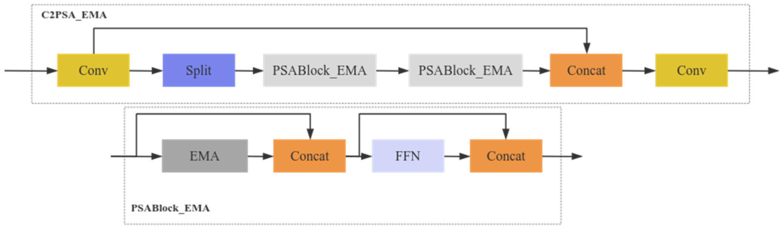
Observations revealed that the localization detection box for targets in supplementary inspections was excessively large with low detection confidence, attributed to insufficient deep semantic information. To address this, the study implemented Efficient Multi-scale Attention (EMA) in the C2PSA module for deep feature processing, replacing the original standard self-attention mechanism in PSA. This approach enables multi-scale feature extraction for deep (P4, P5) features while enhancing the model’s attention focus on target features across different scales. By integrating group coordinate attention with cross-matrix interaction, the mechanism simultaneously captures directional information, local details, and global contextual features, thereby avoiding excessive sequential processing and maintaining optimal depth.

The EMA first divides the input features into $G$ sub-feature groups, each learning distinct semantic representations:

$$F_g=\mathrm{S}\mathrm{p}\mathrm{l}\mathrm{i}\mathrm{t}(X,G), g=1,2,\dots ,G.$$

(13)

In each sub-feature group, the EMA architecture employs three parallel pathways to extract attention weight descriptors from the grouped $F_g$ feature maps. Two 1 × 1 convolutional branches process each subgroup feature, performing one-dimensional global average pooling along both height and width dimensions to encode spatial information.

Height pooling:

$$z_g^h\left(h\right)={\displaystyle \frac{1}{W}}\sum _{0\le w<W}{X}_g\left(h, w\right).$$

(14)

Width direction pooling:

$$z_g^w\left(w\right)={\displaystyle \frac{1}{H}}\sum _{0\le h<H}{X}_g\left(h, w\right).$$

(15)

After concatenating the pooled results, the fully connected layer and activation function GeLU are used to generate attention weights:

$$z_g=\mathrm{G}\mathrm{e}\mathrm{L}\mathrm{U}\left(\mathrm{F}\mathrm{C}\left(Concat\left(z_g^h,z_g^w\right)\right)\right).$$

(16)

Split $z_g$ the weights into height and width directions, then normalize them using the Sigmoid function:

$${\mathrm{\alpha }}_g^h=\sigma \left(z_g^h\right),{\mathrm{\alpha }}_g^w=\sigma \left(z_g^w\right).$$

(17)

Reweight the original features:

$${\tilde{X}}_g=X_g\cdot {\mathrm{\alpha }}_g^h\cdot {\mathrm{\alpha }}_g^w.$$

(18)

For parallel use of 1 × 1 and 3 × 3 convolutional capture of different scale features:

$$F_{1\times 1}=Con{v}_{1\times 1}\left(X_g\right),F_{3\times 3}=Con{v}_{3\times 3}\left(X_g\right).$$

(19)

Cross-scale feature interaction through matrix multiplication:

$$F_{\mathrm{c}\mathrm{r}\mathrm{o}\mathrm{s}\mathrm{s}}=\mathrm{S}\mathrm{o}\mathrm{f}\mathrm{t}\mathrm{m}\mathrm{a}\mathrm{x}\left(F_{1\times 1}·F_{3\times 3}^{\top }\right).$$

(20)

The interaction results are fused with the features after coordinate attention reweighting:

$$Y_g={\tilde{X}}_g+F_{\mathrm{c}\mathrm{r}\mathrm{o}\mathrm{s}\mathrm{s}}·{\tilde{X}}_g.$$

(21)

The final output ensures training stability through residual connections:

$$Y=X+\gamma \cdot Concat\left(Y_1,Y_2,\dots ,Y_G\right).$$

(22)

Here, $\gamma$ is a learnable scaling parameter.

The network structure of the improved C2PSA_EMA module is shown in Figure 5.

3.5. Occlusion Disturbance Processing Based on Collaborative Spatial-Channel Attention

In marine debris detection, multi-objective mutual occlusion severely interferes with localization accuracy. Occlusion results in incomplete target features and introduces a large amount of background and occluding object interference features, making it difficult for general detection heads to accurately regress bounding boxes.

Attention mechanisms like Squeeze-and-Excitation (SE) and Convolutional Block Attention Module (CBAM) sequentially or jointly model channel and spatial importance to refine features. For occlusion handling, these mechanisms can be limited as they may not explicitly model the relationship between visible and occluded parts.

From a formal perspective, we define robustness as the ability of the detector to maintain stable and high detection accuracy when targets are partially occluded. A robust model is expected to show minimal performance degradation under increasing occlusion levels, which is critical for reliable marine debris detection. Let A denote the mAP@0.5 of the model in clean scenes, and $A_0$ denote the mAP@0.5 in occluded scenes. The robustness metric is defined as:

$$R= {\displaystyle \frac{A_0}{A}}$$

(23)

A higher $R$ (closer to 1) means stronger robustness. From quantitative experiments, after applying CSCAM, the mAP@0.5 under occlusion increases from 79.3% to 83.2%, and the robustness score $R$ increases significantly, showing a clear numerical improvement.

Empirical analysis reveals that in occluded scenes, the visible fragments retain the most discriminative cues, whereas occluded regions contribute negligible information and introduce noise. To mitigate this, we propose the Collaborative Spatial-Channel Attention Mechanism (CSCAM), which differs by introducing a collaborative evaluation and fusion strategy specifically designed for occlusion. CSCAM recalibrates feature map significance prior to the detection head, adaptively amplifying signals from visible areas while suppressing interference from occluded parts.

This strategy significantly bolsters model robustness against occlusion. Here, robustness refers to the model’s ability to maintain high detection accuracy when the input data contains partial occlusions that obscure the target objects. Formally, a robust detector should exhibit minimal performance degradation under increasing levels of occlusion. Algorithm 1 presents the detailed procedure of the proposed Collaborative Spatial-Channel Attention Mechanism (CSCAM).

Algorithm 1: A Collaborative Spatial-Channel Attention Algorithm

Input: Feature map F $\in {\mathbb{R}}^{C\times H\times W}$ Output: Enhanced feature map Y $\in {\mathbb{R}}^{C\times H\times W}$

1.   //Get input feature dimensions. 2.    C, H, W = F.shape[1], F.shape[2], F.shape[3] 3.    //Spatial Confidence Level Assessment 4.    //Preliminary spatial confidence level information 5.    Fs_prime = DepthwiseConv2D(F, kernel_size = 1, padding = 0) 6.    Fs = GeLU(Fs_prime) 7.    Fs = BatchNorm(Fs) 8.    //Introduce learnable channel scaling weights to generate the final spatial 9.    confidence weight map. 10.  Fs_conv = Conv2D(Fs, kernel_size = 1, padding = 0) 11.  Fs_conv = GeLU(Fs_conv) 12.  Fs_conv = BatchNorm(Fs_conv) 13.  //Introduce learnable channel scaling weights to generate the final spatial 14.  confidence weight map. 15.  ws = LearnableParameter(shape = (C, 1, 1)) 16.  Ms = Fs_conv * ws 17.  z_s = GlobalAveragePooling(Ms) 18.  //Learning complex nonlinear relationships between channels through a bottleneck 19. structure (fully connected layer). 20. a = ReLU(Linear(z_s, out_features = C//r)) 21. m_c_prime = Linear(a, out_features = C) 22. M_cs = Sigmoid(m_c_prime) 23. //Feature Evaluation, Fusion, and Enhancement 24. M_SC_prime = Ms * M_cs 25. //Expand the disparity between key regions and non-key regions 26. M_SC = exp(M_SC_prime) 27. //Feature Re-weighting and Residual Connection 28. weighted_features = FeatureWeighting(F, M_SC) 29. Y = F + weighted_features 30. Return Y

The complete network architecture of the CSCAM module is illustrated in Figure 6. In this architecture, Fc denotes the fully connected layer, while Fw represents the feature weighting operation through per-channel multiplication. The CSCAM module is designed to enhance focus on visible parts of occluded marine debris and suppress interference from occlusion and background by collaboratively evaluating the importance of spatial and channel dimension features. Its working principle can be decomposed into three core steps: spatial dimension evaluation, channel dimension evaluation, and feature evaluation fusion, collectively achieving the reduction in occlusion interference and enhancement of unoccluded features. Spatial dimension evaluation assigns an initial confidence score to each spatial position in the feature map, assessing the reliability and integrity of features at that location. Channel dimension evaluation evaluates the global importance of each feature channel and suppresses channels with low importance. Feature evaluation fusion integrates the results of spatial and channel evaluations, and enhances important features through nonlinear amplification.

Mapping the given input feature $F\in {\mathbb{R}}^{C\times H\times W}$ map, we first employ deep convolutional feature encoding to extract preliminary spatial confidence information.

$$F_s^{\prime }=DWCon{v}_{k=1}\left(X\right).$$

(24)

The nonlinear transformation of the output spatial reliability information is performed:

$$\mathrm{G}\mathrm{e}\mathrm{L}\mathrm{U}(x)=x\mathrm{\Phi }(x)=x·{\displaystyle \frac{1}{2}}[1+\mathrm{e}\mathrm{r}\mathrm{f}\left({\displaystyle \frac{x}{\sqrt{2}}}\right)],$$

(25)

$$F_s=\mathrm{G}\mathrm{e}\mathrm{L}\mathrm{U}\left(F_s^{\prime }\right).$$

(26)

Among them, erf refers to the Error Function, a special function that cannot be directly expressed using elementary functions. It is defined as the definite integral of the Gaussian function $e^{-t^2}$ from 0 to x, with a value range between −1 and 1. This function has a strict mathematical equivalence relationship with the cumulative distribution function (CDF) of the standard normal distribution. In the GeLU formula you provided, the essence of introducing erf is to apply smooth weighting to the input values using the cumulative probability of the Gaussian distribution; this enables GeLU to retain the sparsity advantages of ReLU while avoiding the non-differentiable points of traditional piecewise functions, providing a smooth and continuously differentiable curve. Consequently, this leads to more stable gradient flow, better nonlinear fitting capability, and superior generalization performance during the training of deep neural networks.

Next, the feature weighting is performed channel by channel, and the spatial confidence map is calibrated according to the global importance of each channel.

$$M_s=F_s\odot w_s.$$

(27)

Here, $w_s\in {\mathbb{R}}^{C\times 1\times 1}$ denotes the learnable channel scaling weight vector, $\odot$ represents the channel-wise multiplication, and $M_s$ is the final spatial confidence weight map.

Then, the spatial confidence weight map is pooled across all channels through full-spectrum averaging, compressing spatial information into a single channel descriptor.

$$z_{\mathrm{c}}^{\mathrm{s}}={\displaystyle \frac{1}{H\times W}}\sum _{h=1}^H\sum _{w=1}^W{M}_{s(c,h,w)},$$

(28)

$$z^{\mathrm{s}}={\left[z_1^{\mathrm{s}},z_2^{\mathrm{s}},\dots ,z_{\mathrm{c}}^{\mathrm{s}}\right]}^T.$$

(29)

The descriptor $z^{\mathrm{s}}$ is fed into a two-layer fully connected bottleneck structure to simulate the complex nonlinear interactions between channels.

$$a=\mathrm{R}\mathrm{e}\mathrm{L}\mathrm{U}\left(W_{1}z+b_1\right),$$

(30)

$$m_{\mathrm{c}}^{\prime }=W_{2}a+b_2.$$

(31)

Here, $W_1\in {\mathbb{R}}^{\left(\frac{C}{r}\right)\times C}$, $W_2\in {\mathbb{R}}^{C\times \left(\frac{C}{r}\right)}$, $r$ is the dimensionality reduction ratio. The first FC layer performs dimensionality reduction and feature fusion, while the second FC layer restores the original dimensions.

The Sigmoid function is then applied for nonlinear transformation $M_c^s$ to derive channel $M_s$ importance weights. These are combined with spatial weights through element-wise multiplication, generating the preliminary collaborative weights.

$$M{\prime }_{SC}=M_S\odot M_C^S.$$

(32)

Apply an exponential function to the collaborative weight to widen the difference between the weights of important and non-important regions:

$$M_{SC}=\exp \left(M_{SC}^{\prime }\right).$$

(33)

Finally, the calibrated collaborative weights are applied to the original input features, with residual connections output to ensure training stability while preserving the original information flow.

$$Y=X+M_{SC}\odot X,Y\in {\mathbb{R}}^{C\times H\times W}.$$

(34)

The improved network structure of the Detect_CSCAM detection head is shown in Figure 7.

4. Experiments and Performance Analysis

4.1. Experimental Setup

The experimental framework operates on the Windows 11 Home operating system, equipped with an NVIDIA GeForce RTX 3060 graphics card produced by NVIDIA, featuring 6 GB of video memory. The software architecture includes CUDA 11.7, Python 3.10.18, and the PyTorch 2.0.0 deep learning framework. The training parameters are configured as follows: the initial learning rate is set to 0.005, batch size is 4, momentum is 0.9, and the number of iterations is 100. The SGD optimizer (with momentum) is employed, and Mosaic data augmentation is applied. The Mosaic augmentation is disabled in the last ten training epochs to facilitate the model’s learning on standard images. An early stopping mechanism is applied with a patience of 10 epochs, monitoring the validation mAP@0.5:0.95. All model implementations maintain consistency in dataset usage and training configurations.

The MD-YOLO model, as well as all baseline models (YOLOv11L, YOLOv9c, YOLOv12l, RT-DETR) used for comparison, were trained from scratch on the Marine_Debris_detect dataset. No pre-trained weights were used for initialization. This choice was made to ensure a fair comparison under identical training conditions and to evaluate the model’s ability to learn features directly from the target domain without external bias.

4.2. Experimental Evaluation

This study uses five metrics to evaluate the performance of supervised object detection models: Precision, Recall, F1-score, mean Average Precision (mAP) at different Intersection over Union (IoU) thresholds, and inference speed (FPS).

All experimental results, including precision, recall, F1-score, mAP@0.5, mAP@0.5:0.95, FPS, GFLOPs, and Params, are tested and calculated under the above unified hardware and software environment to ensure fairness, consistency, and reproducibility.

Before calculating metrics such as Precision, Recall, and F1-score, it is essential to define the basic evaluation criteria. These include True Positives (TP), False Negatives (FN), False Positives (FP), and True Negatives (TN).

Precision is a metric for assessing positive predictions. It represents the proportion of samples predicted as positive that are actually positive. Its calculation formula is shown in Equation (35).

$$Precision={\displaystyle \frac{TP}{TP+FP}}.$$

(35)

Recall rate is an evaluation metric for the original sample, indicating the proportion of samples predicted as positive when they are actually positive. The calculation formula is shown in Equation (36).

$$Recall={\displaystyle \frac{TP}{TP+FN}}.$$

(36)

The precision and recall rates vary with different confidence thresholds. When the confidence thresholds are sufficiently dense, an approximately continuous Precision-Recall curve can be obtained, from whiczh the F₁ score and mean Average Precision (mAP) can be calculated.

The F₁ index is derived from the $F_{\beta }$ index, with its calculation formula as shown in Equation (37). When $\beta$ is greater than 1, the model emphasizes Recall. When $\beta$ is less than 1, the model emphasizes Precision. When $\beta$ equals 1, the result is the $F_1$-score. This demonstrates that the $F_1$-score combines both Recall and Precision, as shown in Equation (38). The value of the $F_1$-score ranges from 0 to 1. A value closer to 1 indicates a better model.

$$F_{\beta }=\left(1+{\beta }^2\right)\times {\displaystyle \frac{Precision\times Recall}{{\beta }^{2}Precision+Recall}}.$$

(37)

$$F_1=2\times {\displaystyle \frac{Precision\times Recall}{Precision+Recall}}.$$

(38)

mAP is a key metric in object detection. It is calculated as the average of the Average Precision (AP) values across all object categories, as shown in Equation (39). In the formula, N denotes the total number of categories to be detected, and AP represents the precision of each category at varying thresholds which calculation formula is shown in Equation (40). This study employs two precision metrics: mAP@0.5 and mAP@0.5:0.95. mAP@0.5 measures the model’s baseline localization performance at a 0.5 IoU threshold, and mAP@0.5:0.95 averages the model’s performance across IoU thresholds from 0.5 to 0.95.

$$mAP={\displaystyle \frac{{\sum }_{n=1}^{N}A{P}_n}{N}},$$

(39)

$$AP={\int }_0^{1}p(r)dr.$$

(40)

FPS (Frames Per Second) measures a model’s inference speed. Its value indicates how many images or video frames the model can process each second. This metric reflects the model’s real-time performance. The calculation formula is shown in Equation (41):

$$FPS={\displaystyle \frac{1000}{t_{pre\text{-}process}+t_{inference}+t_{NMS}}}.$$

(41)

The three time components in the denominator represent preprocessing time ($t_{pre\text{-}process}$), inference time ($t_{inference}$), and post-processing time ($t_{NMS}$). All time is measured in milliseconds (ms).

The confusion matrix visualizes classification efficacy, with the main diagonal indicating per-class accuracy. Crucially, the distribution of off-diagonal errors highlights specific failure modes, facilitating a deeper understanding of where and why the model struggles.

4.3. Performance of MD-YOLO Network

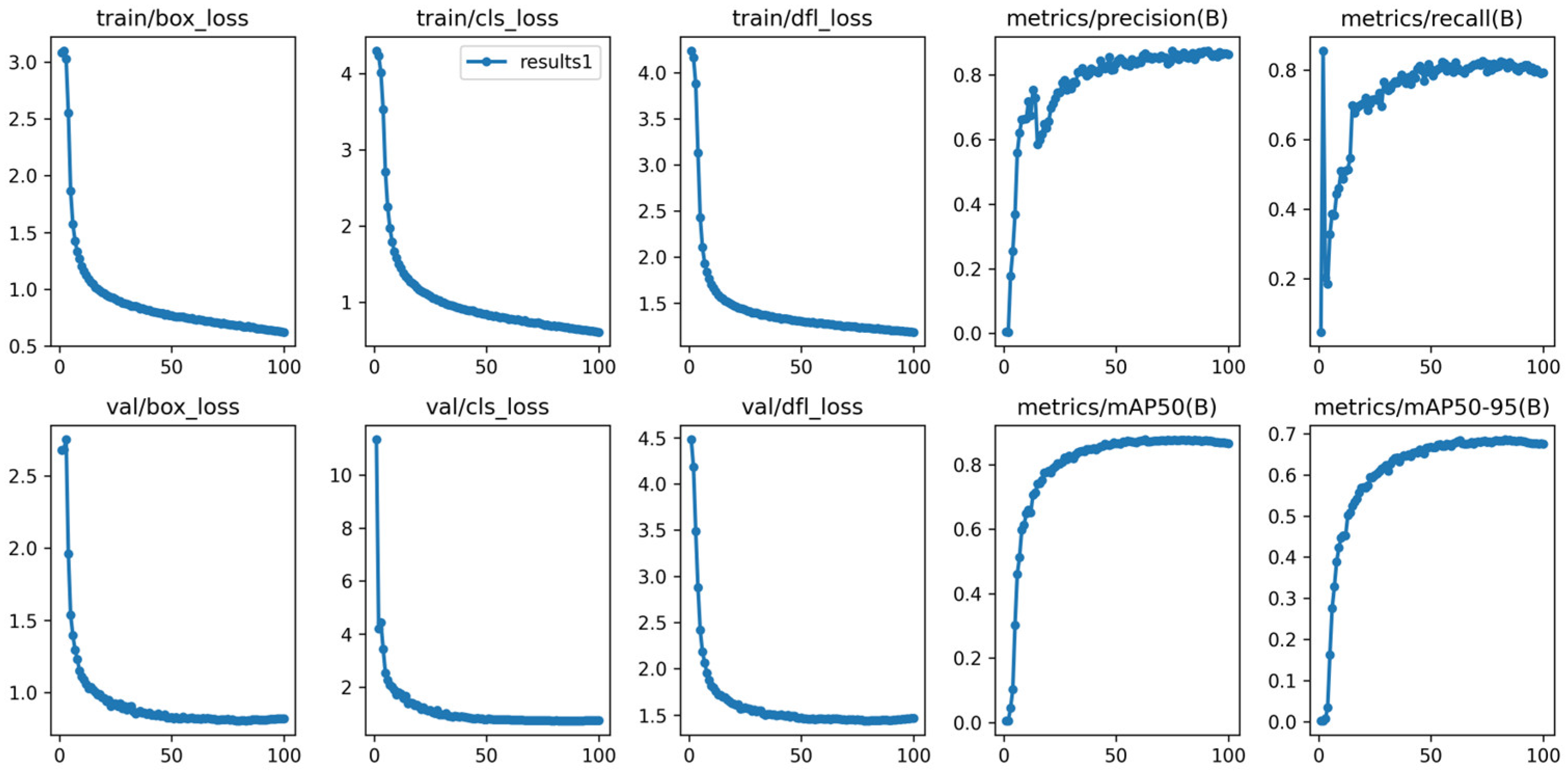
As depicted in Figure 8, the loss curves follow a characteristic decay pattern, rapidly minimizing before stabilizing. Crucially, the validation loss mirrors the training loss throughout the process, confirming that the model captures generalizable features rather than memorizing noise. This effective learning translates directly into performance metrics—Precision and Recall rise in tandem, achieving a high-level equilibrium. Furthermore, the marked improvements in mAP50 and mAP50–95 validate the model’s robustness, demonstrating its capability to maintain high accuracy even under strict localization criteria. It excels at locating marine debris and producing high-quality, precise bounding boxes.

4.4. Ablation Experiment

To validate the effectiveness of the proposed improvements in MD-YOLO for enhancing model performance, an ablation experiment was conducted. In this experiment, images were input at 640 × 640 resolution, and the baseline model was YOLOv11L. Different combinations of four improvement points were tested, with eight additional experiments designed alongside the baseline: (1) YOLOv11L + MSCM; (2) YOLOv11L + EMA; (3) YOLOv11L + CSCAM; (4) YOLOv11L + DAT; (5) YOLOv11L + MSCM + EMA; (6) YOLOv11L + DAT + CSCAM; (7) YOLOv11L + MSCM + EMA + CSCAM; (8) YOLOv11L + MSCM + EMA + CSCAM + DAT. The results of the ablation experiments are presented in

Table 4. Results of Ablation Experiments on the Marine_Debris_detect Dataset.

Model	mAP@0.5	mAP@0.5:0.95	F1	FPS	GFLOPs	Params (M)
YOLOv11L (Baseline)	79.3%	61.4%	0.76	51.8	87.3	25.3
+MSCM	79.5%	61.7%	0.76	52.9	83.7	25.1
+EMA	80.4%	62.2%	0.77	45.7	87.5	25.4
+CSCAM	82.8%	62.9%	0.80	35.7	88.0	25.5
+DAT	81.0%	61.9%	0.78	52.6	90.8	26.4
+MSCM + EMA	81.4%	62.4%	0.78	50.3	83.9	25.2
+CSCAM + DAT	83.7%	64.1%	0.81	38.5	91.5	26.6
+MSCM + EMA + CSCAM	85.3%	65.9%	0.82	37.0	84.6	25.3
MD-YOLO (ours)	86.7%	67.6%	0.83	39.8	88.1	26.4

. A + indicates that the method was added to YOLOv11L for improvement in the respective experiment.

The experiments demonstrate that implementing the Multi-scale Convolution Module (MSCM) at the backbone’s P3 node significantly enhances overall model performance. The mAP@0.5 and mAP@0.5:0.95 metrics improved by 0.2% and 0.3%, respectively, with FPS increasing by 1.1. This improvement stems from the multi-scale convolutional network’s ability to efficiently extract features of varying sizes. The integration of the efficient multi-scale attention mechanism (EMA) significantly enhances the backbone network through its coordinate channel attention mechanism and matrix cross-attention fusion. The upgraded model demonstrates superior recognition performance and efficiency, achieving a 2.1% improvement in mAP@0.5 and a 1.0% increase in mAP@0.5:0.95 compared to the original model. Marine debris detection is severely hindered by object occlusion, which degrades localization accuracy. To address this, we introduced a context-aware multi-scale feature fusion strategy alongside the Collaborative Spatial-Channel Attention Mechanism (CSCAM). By explicitly extracting unoccluded features and inferring occluded regions through contextual cues, this combination yielded immediate gains: mAP@0.5 and mAP@0.5:0.95 increased by 3.9% and 3.5%, respectively, with the F1 score rising by 0.04. This performance leap directly quantifies the enhanced robustness against occlusion provided by CSCAM.

Building on this foundation, we integrated a Deformable Attention Mechanism (DAT) at the P4 neck node to enable dynamic sampling. This refinement further boosted performance, adding 1.4% to mAP@0.5 and 1.7% to mAP@0.5:0.95, while also increasing inference speed by 2.8 FPS.

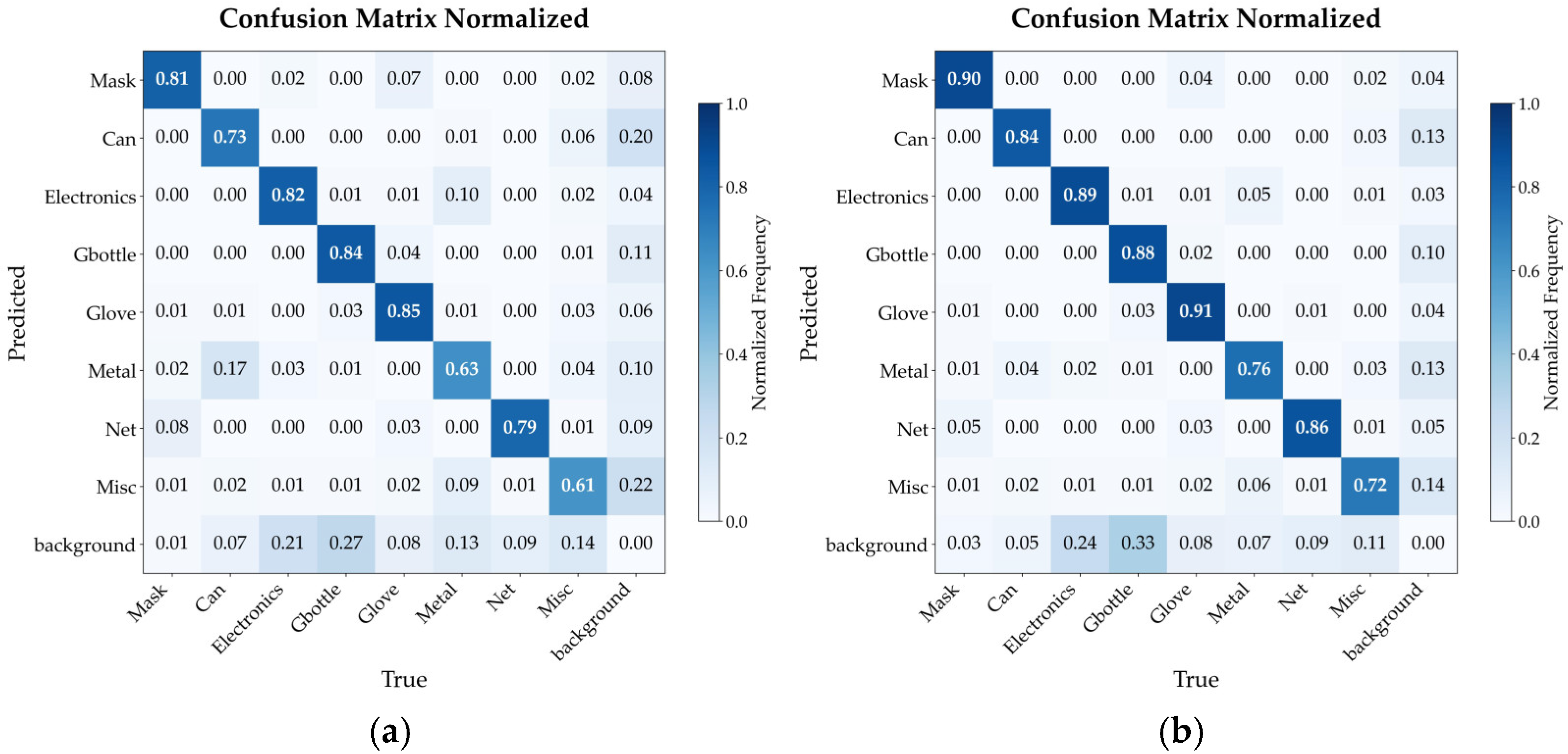
Cumulatively, our improved MD-YOLO model outperforms the baseline YOLOv11L with substantial margins: +7.4% in mAP@0.5, +6.2% in mAP@0.5:0.95, and +0.07 in F1 score. While these accuracy gains came with a modest speed trade-off, the model maintains 39.8 FPS, well above the 24 FPS threshold required for real-time applications. As confirmed by the confusion matrix (Figure 9), MD-YOLO achieves a marked gain in mAP@0.5:0.95 over YOLOv11L, underscoring its enhanced localization precision when evaluated under stringent IoU thresholds. MD-YOLO achieves superior localization precision across all debris categories, effectively validating our approach to balance the classic speed–accuracy trade-off in complex marine environments.

4.5. Comparative Experiments

To further validate the superiority of the MD-YOLO model proposed in this chapter, we conducted comparative experiments with mainstream detection models using the Marine_Debris_detect dataset. The experimental group comprised two-stage recognition model Faster R-CNN, one-stage recognition models YOLOv9c and YOLOv12l [44], and transformer-based Real-Time Detection Transformer (RT-DETR). The results are presented in

Table 5. Performance Comparison of Different Models on the Marine Debris Dataset.

Model	mAP@0.5	mAP@0.5:0.95	F1	FPS	GFLOPs	Params (M)
Faster R-CNN	83.6%	65.3%	0.81	18.3	370.2	137.1
YOLOv9c	80.3%	59.1%	0.78	47.6	84.8	21.5
YOLOv12l	79.1%	58.8%	0.77	49.4	88.6	26.3
RT-DETR-r34	81.2%	61.1%	0.79	51.2	88.9	30.3
MD-YOLO	86.7%	67.6%	0.83	39.8	88.1	26.4

.

The comparative results in the table demonstrate that the MD-YOLO model proposed in this chapter exhibits outstanding comprehensive performance. The Faster R-CNN model achieves recognition accuracy comparable to MD-YOLO, with mAP@0.5, mAP@0.5:0.95, and F₁ score reaching 83.6%, 65.3% and 0.81, respectively, indicating excellent recognition accuracy. However, its two-stage detection workflow significantly reduces recognition speed, with only 18.3 FPS, failing to meet real-time requirements. Additionally, its computational floating-point operations and parameter volume are several times higher than MD-YOLO, substantially increasing computational resource consumption. The single-stage models YOLOv9c and YOLOv12l achieve comparable efficiency to MD-YOLO, with FPS of 47.6 and 49.4, GFLOPs of 84.8 and 88.6, and parameters of 21.5 M and 26.3 M, respectively. While conserving computational resources, they maintain good real-time performance. However, their mAP@0.5 and mAP@0.5:0.95 scores are only 80.3%, 59.1% and 79.1%, 59.8%, respectively, failing to meet engineering requirements for detection accuracy. As a classic research model in current detection approaches, RT-DETR-r34 simplifies training and inference processes through its end-to-end improvement without requiring NMS post-processing. Despite its simplified end-to-end pipeline, RT-DETR-r34’s performance remains substantially lower than that of MD-YOLO, while its training is typically more resource-intensive. The MD-YOLO proposed in this chapter outperforms other detection models by combining high localization accuracy with faster inference speed. Its reduced computational floating-point operations and parameter size further minimize resource demands, delivering outstanding comprehensive performance. The ceiling on performance of its mAP@0.5:0.95 is only 67.6% can be attributed to several inherent difficulties in the dataset and task. On the one hand, objects like Misc encompass diverse shapes, and debris can be highly deformed or degraded, making consistent feature learning difficult. On the other hand, in dense debris piles, even human annotators may struggle to precisely delineate every object, leading to inherent ambiguity in ground truth and a performance upper bound.

4.6. Visualization Experiment

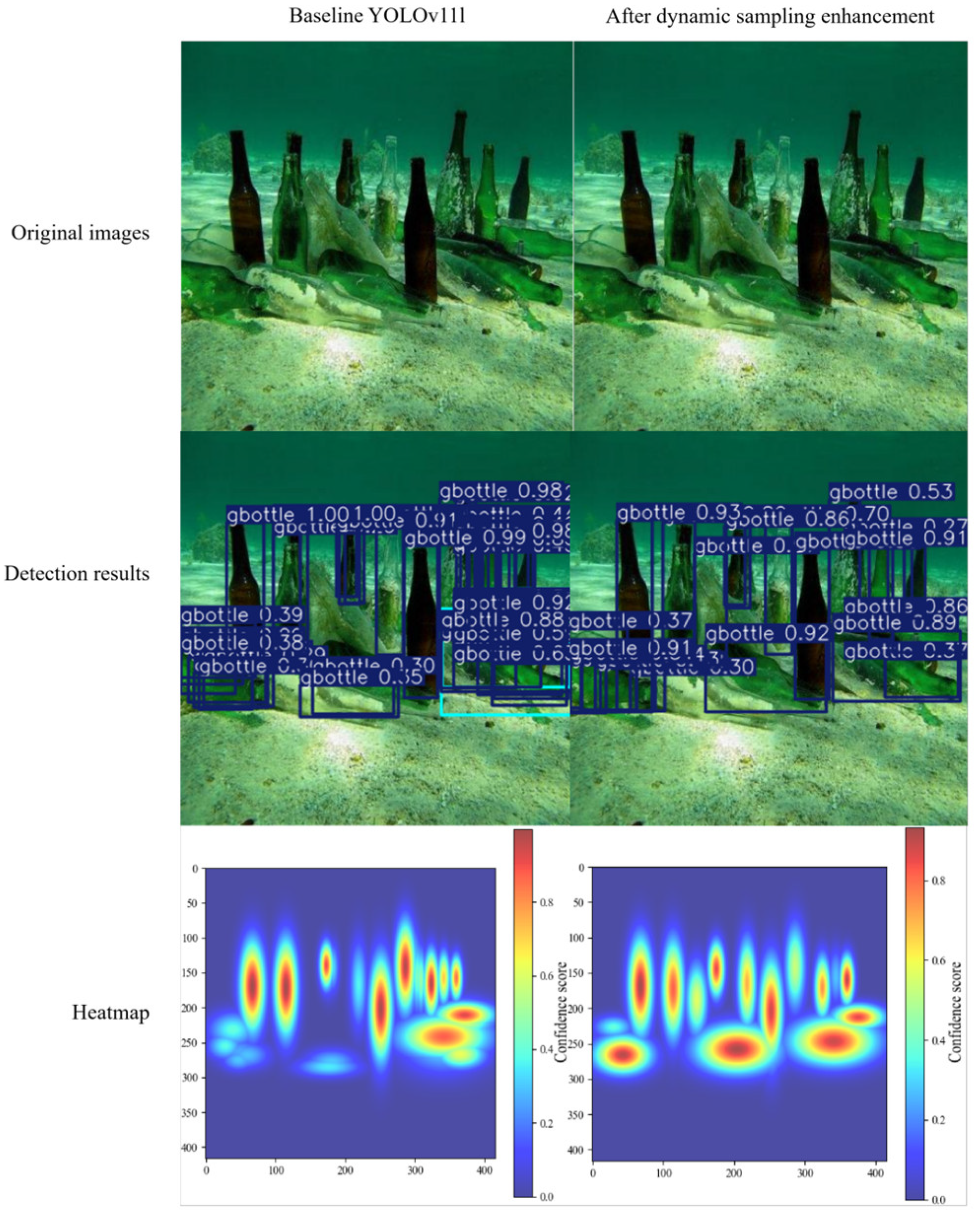
Figure 10 shows that in the original YOLOv11L model’s detection process, glass bottles with imbalanced aspect ratios caused detection dispersion and false positives, erroneously classifying single objects as multiple targets. This significantly compromised detection accuracy while generating bounding boxes with substantial offsets. Through dynamic sampling optimization, high-confidence points now concentrate on the bottle’s structural integrity, forming complete activation zones that produce both highly confident and precisely aligned bounding boxes. This paper’s dynamic sampling-based optimization effectively resolves issues of out-of-focus box localization and excessive bounding range in irregular waste detection.

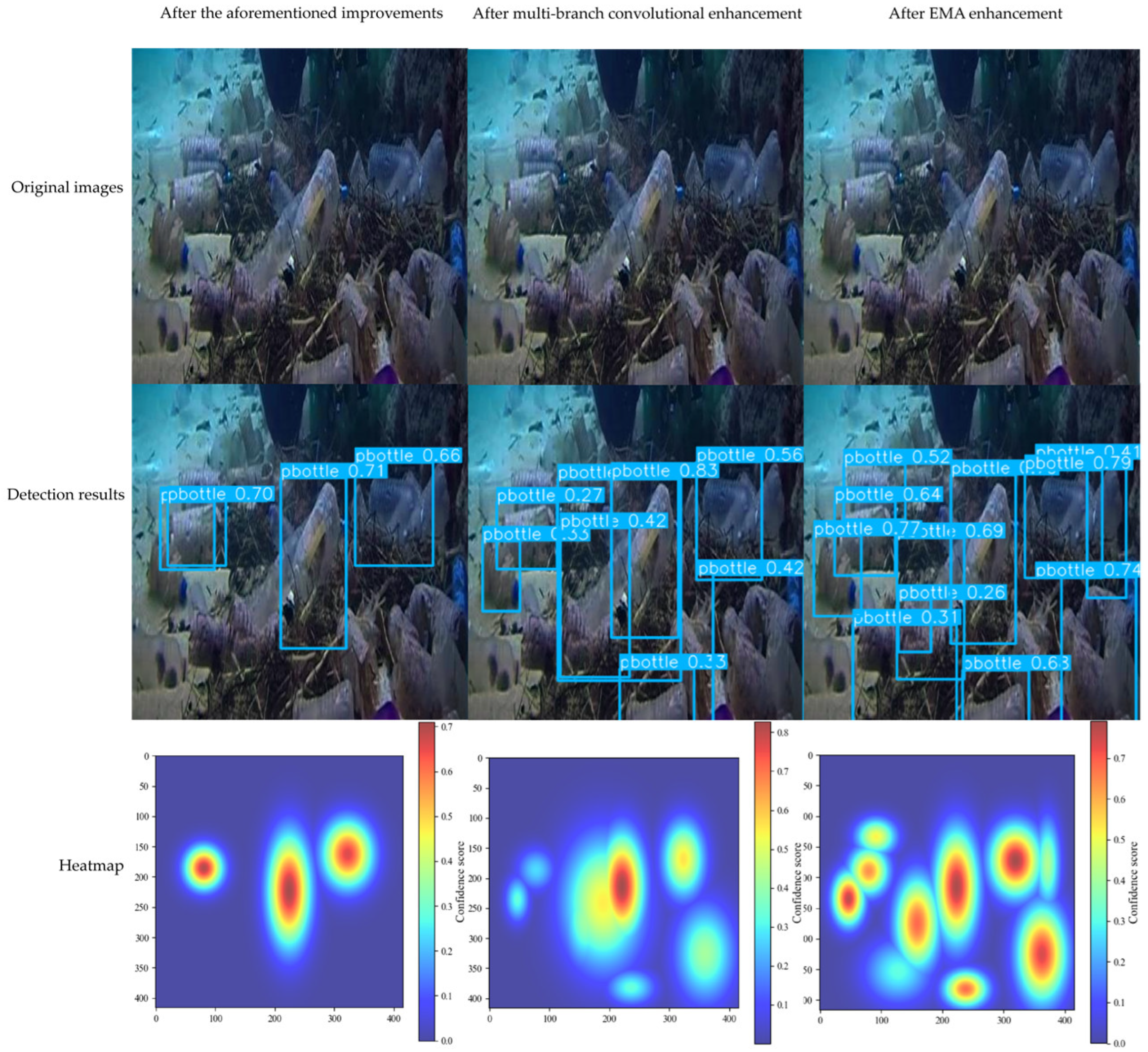
Figure 11 shows a comparison of detection results before and after the improvement of multi-scale feature extraction. After the dynamic sampling enhancement, the model can completely detect heterogeneous objects. However, when objects of significantly different sizes coexist in an image, the detection confidence is affected due to the failure to recognize small objects, mainly because the presence of larger objects distracts the model’s attention from smaller ones. The model improved with multi-branch convolution as it successfully detected multiple previously missed pieces of trash. Subsequently, applying EMA to reweigh the attention weights of the extracted deep features not only retains rich local details but also considers global semantics. This provides the network with multi-scale analysis and localization information, further detecting multiple missed trash items. The experiment demonstrates that the enhanced model effectively addresses detection blind spots in scenes where multi-sized trash objects coexist.

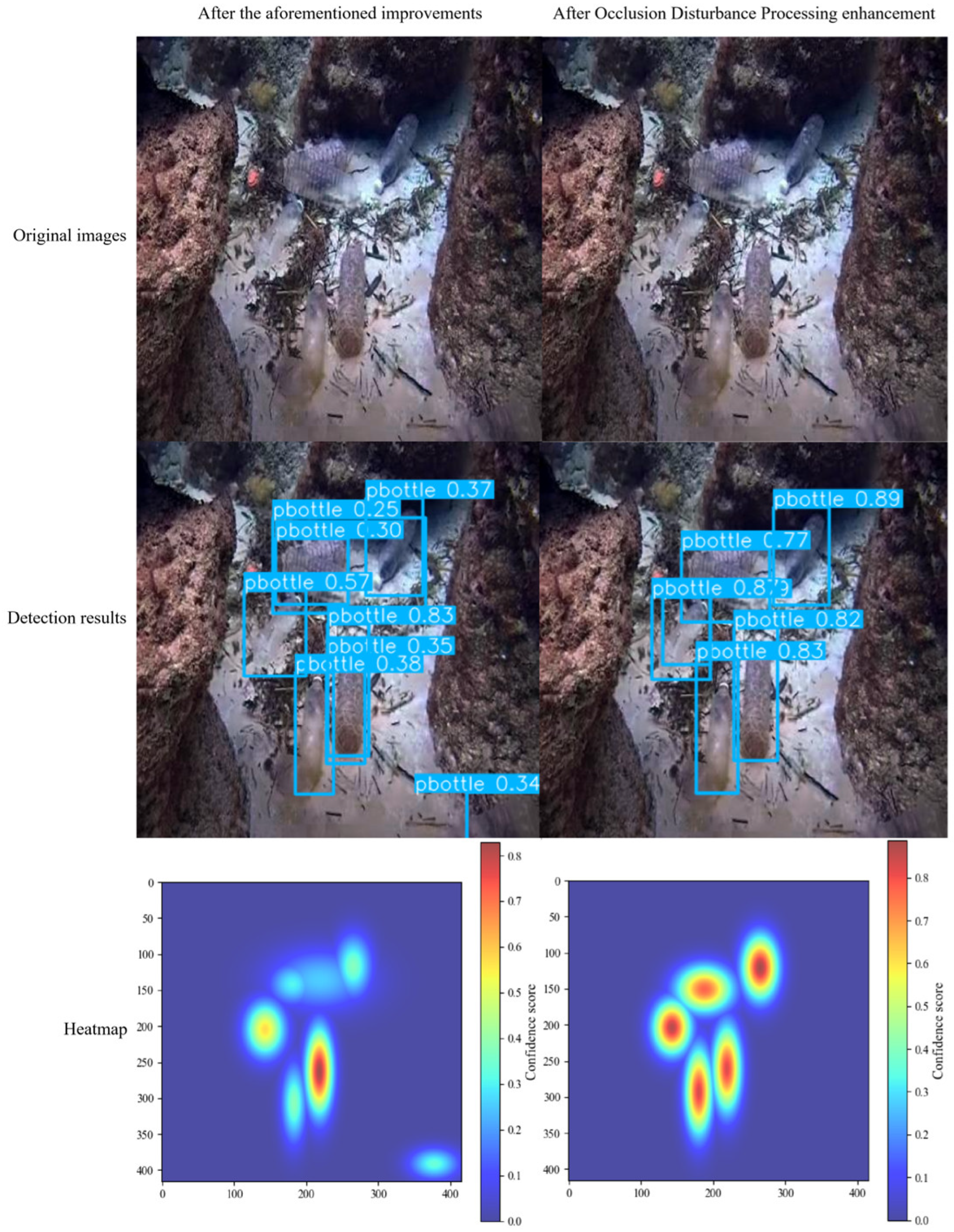
Figure 12 presents a comparison of detection results before and after the improvement in occlusion interference handling.

After the previous enhancements, a bottle occluded by trash in front of it shows a weak response in the heatmap, receiving limited attention. This restricts its feature localization area, leading to a relatively low detection confidence of only 0.3. After optimization for occlusion interference, the model’s robustness to occlusion is significantly enhanced. The unobstructed part of the bottle in the heatmap is activated, and the model’s focus area expands and concentrates accordingly, thereby generating a more precise bounding box. Consequently, the corresponding detection confidence increases substantially to 0.77.

This series of experiments systematically validates the effectiveness of three improvement strategies: deformable sampling enhancement, context-aware multi-scale feature extraction, and attention-based occlusion handling. These enhancements, respectively, address three core challenges in marine object detection: feature consistency, scale sensitivity, and occlusion robustness.

(1)

Deformable sampling enhancement improves the stability of the model’s perception at the data level.

(2)

Multi-scale feature extraction optimization (multi-branch convolution + EMA) enhances the model’s discriminative power for targets of different sizes at the network architecture level.

(3)

The cooperative spatial-channel attention mechanism improves the model’s reasoning capability under local information deficiency (occlusion) at the feature optimization level.

Our experiments confirm that the proposed strategies act synergistically within the YOLOv11L framework. This integration yields a robust detector specifically tailored for complex marine environments, delivering substantial gains in scenarios characterized by drastic scale variations and severe mutual occlusion. These advancements bridge the gap between theoretical model improvements and the demanding requirements of real-world marine monitoring systems.

5. Conclusions and the Future Work

5.1. Conclusions

This work tackles the challenge of marine debris detection in complex oceanic environments. Our primary objective is to develop a high-precision model capable of overcoming three critical bottlenecks: extreme aspect ratios, drastic scale variations, and severe mutual occlusion.

To this end, we propose MD-YOLO, an enhanced architecture featuring three strategic innovations. First, we integrate Deformable Convolution into the P4 neck layer, enabling dynamic feature sampling that adapts to irregular object shapes. This specifically mitigates background noise and enhances localization for debris with highly elongated geometries. Second, we redesign the P3 backbone layer with a multi-branch convolutional structure, synergized with an efficient attention mechanism within the C2PSA module. This dual approach ensures a robust balance between fine-grained local details and global contextual information, significantly improving multi-scale feature representation. Finally, a collaborative spatial-channel attention mechanism is designed in the detection head to adaptively suppress occluded regions while inferring their positions using contextual information, thereby improving robustness for marine debris localization under occlusion. Experimental results demonstrate that the improved MD-YOLO model achieves significant performance gains on the self-built Marine_Debris_detect dataset, with improvements of 7.4%, 6.2% and 0.07 in mAP@0.5, mAP@0.5:0.95, and F₁ score, respectively, compared to the original YOLOv11L model, effectively validating the model enhancement’s impact on marine debris localization accuracy.

5.2. The Future Work

The MD-YOLO model proposed in this paper, by incorporating deformable convolution, multi-branch structures, and a collaborative attention mechanism, has achieved significant performance improvements on the self-built marine debris detection dataset in addressing challenges such as aspect ratio imbalance, multi-scale coexistence, and occlusion. However, the application of marine debris localization in complex marine scenes still faces numerous challenges. Future work can be further advanced in the following directions.

Co-optimization of model architecture and efficiency: While the current improvements enhance accuracy, they inevitably increase model complexity and computational overhead. Future research could explore more efficient deformable operations and dynamic sparse attention mechanisms to significantly reduce parameter counts and inference latency while maintaining or even improving performance, thereby meeting the real-time deployment requirements of mobile or embedded devices. Furthermore, investigating adaptive network structures that dynamically adjust computational resources based on input image complexity will be a crucial approach to achieving the optimal trade-off between accuracy and efficiency.

Moving beyond static imagery, future iterations of MD-YOLO will target spatiotemporal consistency and 3D reconstruction. Incorporating temporal modeling will mitigate artifacts like motion blur and transient occlusion in video streams, ensuring robust tracking. Furthermore, bridging the gap to 3D perception via monocular depth priors or multi-modal sensor fusion (e.g., sparse point clouds) will enable 6D pose estimation. These advancements are pivotal for transitioning from passive detection to active manipulation in unstructured marine environments.