Collision Avoidance Path Optimization for Unmanned Surface Vessels Integrating Velocity Obstacle Method and Improved CVaR Under Uncertainty Modeling

Abstract

Planning effective collision avoidance routes is a crucial measure for ensuring ship safety. However, position uncertainty caused by sensor noise, communication delays, and sudden changes in the maneuvering of target vessels severely restricts the reliability of traditional collision avoidance methods. To address this, this study integrates the velocity obstacle method and conditional value at risk theory to design a ship collision avoidance framework under position uncertainty. The position uncertainty of the target vessel is modeled using a Gaussian distribution. By fusing multi-source sensor data from radars and the Automatic Identification System through Bayesian inference, the posterior estimate of the vessel’s position is dynamically updated, thereby constructing an uncertainty velocity obstacle region. The Gaussian posterior distribution of the position is incorporated into a stochastic loss function to formulate a stochastic optimization model that balances navigation efficiency and collision risk. The model is solved using the sample mean approximation method and strictly complies with the International Regulations for Preventing Collisions at Sea. The results of two sets of multi-vessel encounter simulations demonstrate that, compared with traditional methods, the proposed method achieves superior performance in terms of total path length and algorithm runtime. It is capable of generating compliant collision avoidance strategies in complex dynamic crossing scenarios, attaining optimal comprehensive performance with respect to safety, economy, and regulatory compliance.

1. Introduction

In recent years, with the rapid development of artificial intelligence, automatic control, and marine information technology, unmanned surface vessels (USVs) have demonstrated broad application prospects in fields such as marine resource exploration, maritime surveillance, port logistics, and search and rescue operations due to their ability to operate continuously for extended periods without a human crew [1,2]. However, the marine environment in which USVs operate is highly dynamic and uncertain, with dense vessel traffic and complex collision scenarios [3]. How to achieve safe, compliant, and efficient autonomous collision avoidance decision-making under these conditions has become a core technical bottleneck hindering the practical deployment of USVs, and it is also a major topic of shared interest in both academic and engineering circles domestically and internationally.

In the field of autonomous collision avoidance for unmanned vessels, researchers have proposed various methods. Early studies predominantly employed the artificial potential field method [4], which models obstacles as repulsive fields and guides the vessel around obstacles via the potential field gradient. While this method offers the advantage of computational simplicity, it is prone to getting stuck in local optima and struggles to handle dynamic targets. Intelligent optimization methods such as particle swarm optimization [5] and genetic algorithms [6] avoid the local optimum problem through global search, but their high computational cost makes it difficult to meet the real-time requirements of collision avoidance; model predictive control (MPC) [7] methods can explicitly handle multiple constraints and offer certain advantages in the coordinated optimization of path tracking and collision avoidance, but they are highly dependent on the accuracy of the target vessel’s motion model. The velocity obstacle (VO) method was proposed by Fiorini et al. in 1998 [8], initially applied in the field of mobile robots, and has been widely adopted in unmanned vessel collision avoidance research in recent years. This method constructs collision regions in velocity space, transforming multi-object collision avoidance into a problem of finding a feasible set of velocities. It offers the advantages of geometric intuitiveness, strong real-time performance, and ease of extension to multi-vessel scenarios, making it one of the mainstream frameworks in current research on autonomous collision avoidance for unmanned vessels [9].

However, traditional VO methods have a significant limitation: they are based on the assumption that the target vessel’s position is precisely known [10]. In actual navigation, unmanned vessels rely entirely on sensors and communication systems to obtain environmental information. Radar suffers from limited range resolution and interference from echo noise, while the AIS system has shortcomings such as low data update rates and signal loss. Furthermore, the effects of wind, waves, and currents in the marine environment introduce significant uncertainty into the target vessel’s motion, resulting in a non-negligible discrepancy between the acquired position data and the actual value [11]. If a collision avoidance decision-making system treats uncertain position data as precise values, the planned collision avoidance maneuvers may pose serious safety risks during actual execution. Excessively tight evasion maneuvers are highly likely to result in actual collision risks exceeding expectations when position deviations are significant [12]. Therefore, how to scientifically quantify the uncertainty of the target vessel’s position and effectively incorporate it into the collision avoidance decision-making framework is key to enhancing the robustness of unmanned vessel collision avoidance systems.

In response to the aforementioned issues, scholars have conducted a series of explorations in recent years. Autonomous collision avoidance for unmanned vessels has evolved from simple geometric reachability analysis to an integrated decision-making framework that combines rule-based constraints, risk assessment, and closed-loop control [13]. Qu et al. proposed a real-time collision avoidance method for emergency encounter scenarios that flexibly complies with International Regulations for Preventing Collisions at Sea (COLREG), and enhanced the algorithm’s safety margin through an expandable obstacle set under conditions of uncertainty in the target vessel’s motion [14]. Zhang et al. further integrated target vessel intent information and quaternion-based vessel domains into a model predictive control framework, balancing regulatory compliance and trajectory feasibility in multi-vessel cooperative collision avoidance [15]; Zhang et al. proposed an autonomous collision avoidance decision support method based on maneuver process deduction, further strengthening the integration between encounter process reasoning and regulatory constraints [16]. These studies indicate that the coupled modeling of navigation rules, intention prediction, and control constraints has become a key direction for enhancing the practicality of unmanned vessel collision avoidance.

On the other hand, uncertainty risk modeling and data-driven decision-making are emerging as key growth areas in this field. Xin et al. developed a method for assessing the probability of multi-vessel collisions based on AIS data that accounts for spatiotemporal motion uncertainty, providing a probabilistic tool for quantifying collision risks in complex traffic flow environments [17]. In the data-driven direction, Mei Huang et al. enhanced autonomous decision-making capabilities in high-density traffic environments from two perspectives: uncertainty-aware reinforcement learning and multi-vessel deep reinforcement learning decision-making [18]. However, reinforcement learning methods remain dependent on the scale of training samples, reward function design, and generalization ability, and their decision interpretability and safety boundary verification are relatively insufficient [19,20]. Some studies employ probability distributions to describe the randomness of a target vessel’s position, introducing uncertainty into the VO framework by expanding the collision region [21]. Regarding sensor fusion, Bayesian inference and Kalman filtering are used to fuse multi-source heterogeneous sensor information to obtain more reliable estimates of the target’s state [22]; regarding risk metrics, conditional value at risk (CVaR) has garnered attention due to its sensitivity to tail-end extreme risks. CVaR not only measures the average loss exceeding a risk threshold but also explicitly constrains collision losses under worst-case scenarios [23]. Hakobyan et al. combined CVaR with motion control, achieving beneficial progress in the field of stochastic collision avoidance [24]. However, most existing studies address uncertainty modeling, multi-sensor fusion, and collision avoidance speed optimization in isolation, lacking a systematic approach that organically integrates these three aspects. Furthermore, the majority of studies still employ deterministic objective functions during the risk optimization phase, failing to simultaneously address the trade-off between navigation efficiency and collision safety within a stochastic optimization framework.

In terms of practical implementation, recent research has begun to place greater emphasis on verifying the robustness of algorithms and ensuring their usability on actual vessels. Madsen et al. discussed the issue of decision transparency in autonomous maritime collision avoidance systems from the perspective of human–machine collaboration, pointing out that high-risk autonomous decision-making requires not only identifying the optimal action but also providing operators with clear explanations of risks and the rationale behind the actions [25]. de Lima et al. conducted comparative validation of various COLREG-compliant collision avoidance algorithms on a real-ship platform, demonstrating that collision avoidance performance evaluation should simultaneously consider comprehensive metrics such as minimum encounter distance, course deviation, and mission completion time [26]. Overall, while existing research has made significant progress in rule compliance, risk assessment, and intelligent decision-making, there remains a gap in characterizing stern-end risks under the combined effects of sensor noise, communication delays, and sudden changes in target vessel maneuvers. This gap provides a clear theoretical and engineering rationale for further research into the introduction of improved CVaR methods.

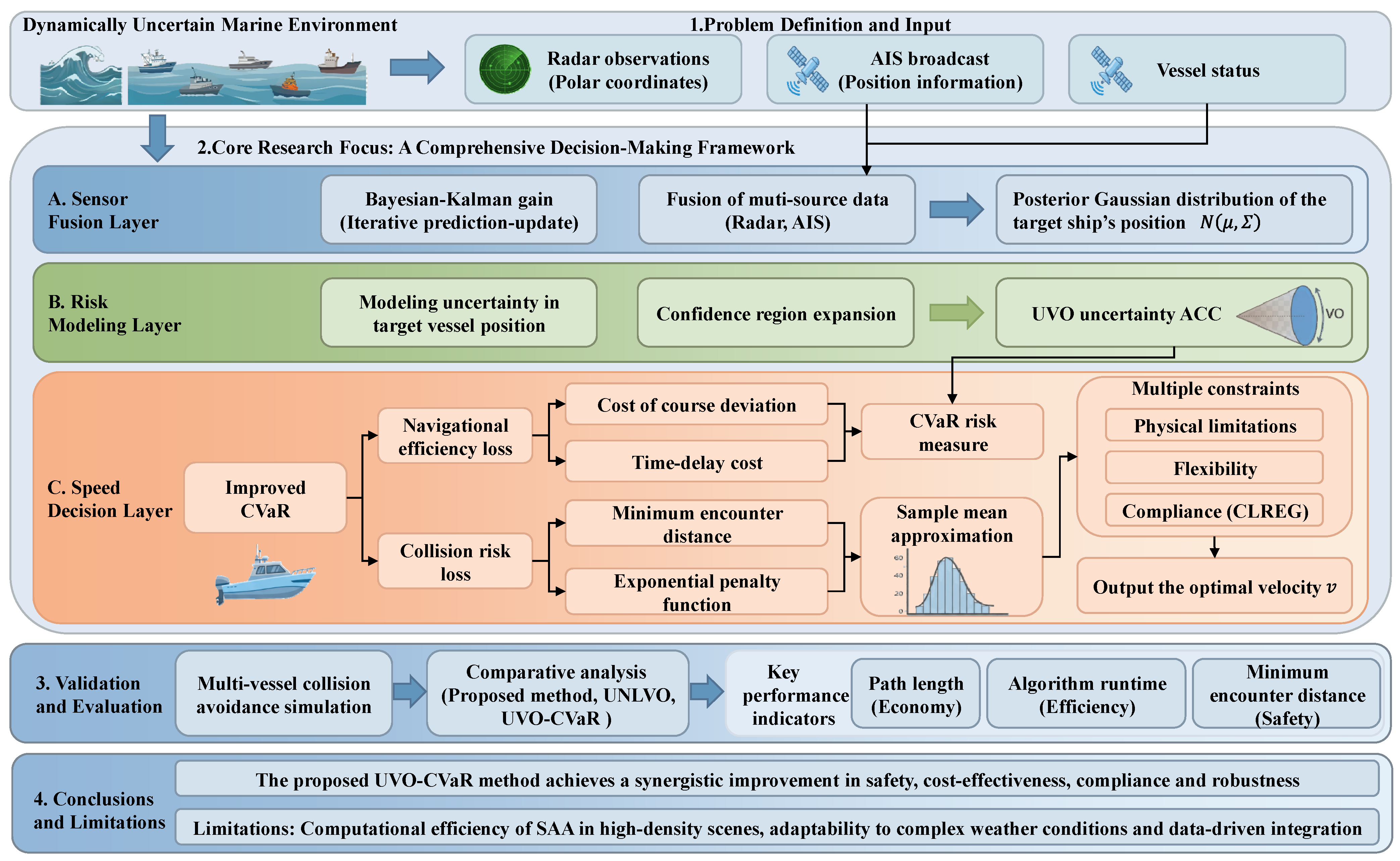
This study builds upon our previous work on the UVO-CVaR collision avoidance framework, in which the uncertainty-aware velocity obstacle model, Bayesian fusion mechanism, collision warning strategy, and baseline CVaR-based speed selection framework were established. In the present paper, these components are retained only as the necessary methodological foundation. The main focus is placed on the proposed improved CVaR method, where the Gaussian posterior distribution of target vessel position is directly embedded into the loss function to construct a stochastic risk-aware speed optimization model, which is then solved by the sample average approximation method. To this end, this study proposes a collision avoidance path optimization method for unmanned vessels based on an improved CVaR approach. A comprehensive decision-making framework was established, encompassing uncertainty modeling, multi-sensor fusion, and robust velocity optimization. The technical workflow is illustrated in Figure 1. Specifically, first, a two-dimensional normal distribution-based uncertainty model for the target vessel’s position is established. A time-varying covariance matrix is used to describe the diffusion pattern of positional prediction errors, and an expanded collision region accounting for the confidence level is constructed based on the Mahalanobis distance, thereby effectively incorporating uncertainty into the velocity constraint framework. Second, a Bayesian inference mechanism is introduced to fuse radar polar coordinate transformation observations with direct AIS position observations using accuracy-weighted integration. Using the normal distribution prediction results as prior information, iterative prediction and updating are performed via a Kalman gain to obtain a posterior estimate of the target vessel’s position, and the uncertainty radius parameters are adaptively updated based on this estimate. Finally, based on the above fusion results, a total loss function is constructed comprising deterministic navigation-efficiency loss terms and stochastic collision-risk loss terms. A stochastic speed optimization model is established using CVaR as the risk metric, and the sample mean approximation (SAA) method is employed for its discrete solution. Under the constraints of maximum speed, dynamic window maneuverability, and the directional constraints of the COLREG (International Regulations for Preventing Collisions at Sea), a robust optimal collision avoidance velocity vector is put out. Through multi-vessel collision avoidance simulation experiments, the proposed method was compared with the baseline UVO-CVaR method and the UNLVO method, verifying that the research method can significantly reduce the total length of the navigation path and decrease algorithm runtime while ensuring safe encounter distances for all target vessels, thereby balancing collision safety and trajectory efficiency.

2. Kinematics and Collision Avoidance Theory Modeling for Unmanned Vessels

2.1. Kinematics Model of an Unmanned Vessel

To describe the planar motion of the unmanned surface vessel, a widely used three-degree-of-freedom model is adopted in this study, including surge velocity, sway velocity, and yaw rate [27]. This model is employed as the basic motion description for subsequent collision avoidance decision-making and path optimization. The corresponding state variables are defined in the body-fixed and earth-fixed coordinate systems, respectively, focusing solely on the relationships among the vehicle’s forward speed u, lateral drift speed v, and yaw rate r, as shown in Figure 2.

2.2. Velocity Obstacle Method

The velocity obstacle method is a collision avoidance algorithm for mobile robots proposed by Fiorini et al. in 1998. This method can also be applied to address collision issues involving unmanned vessels. First, the unmanned vessel is abstracted as a circle; second, for the sake of convenience in analysis, the radius and velocity of the home vessel are superimposed onto the target vessel. Through this transformation, the complex multi-target motion collision avoidance problem is reduced to a single-target motion collision avoidance problem. Finally, two tangents are drawn from the home vessel’s position O to the target vessel’s region T. If the combined velocity vector of the home vessel and the target vessel falls within this region, it implies that the two vessels will collide at some point in time [28,29]. The region between these two tangents is called the relative collision region (RCC) as shown in Figure 3a and can be expressed as:

$$RCC=\left\{v_{\mathrm{rel}}\in {\mathrm{R}}^2\left|\exists t\right.>0,v_{\mathrm{rel}}\in T\ominus O\right\}$$

(1)

where $v_{\mathrm{rel}}=v_{\mathrm{OS}}-v_{\mathrm{TS}}$ represents the relative velocity, $v_{\mathrm{OS}}$ and $v_{\mathrm{TS}}$ represent the velocity vectors of the home vessel and the target vessel, respectively, and $\ominus$ represents the Minkowski difference operator, $\mathrm{R}$ denotes the set of real numbers.

To better study multi-vessel collision scenarios, the relative collision region is transformed into an absolute collision region (ACC) as shown in Figure 3b, which is the set of speed vectors of the vessels involved that lead to the collision:

$$ACC=\left\{v_{\mathrm{OS}}\in {\mathrm{R}}^2\left|v_{\mathrm{OS}}\in \lambda (v_{\mathrm{rel}})\oplus \left(\mathrm{T}\ominus \mathrm{O}\right)\right.\right\}$$

(2)

The ACC is a set of velocity vectors representing collisions between the vessel and target vessels. $\oplus$ denotes the Minkowski inner product, and $\lambda \left(v_{\mathrm{rel}}\right)$ is the ray originating from the origin and extending in the direction of $v_{\mathrm{rel}}$. When conducting multi-vessel collision avoidance studies, all ACCs must be considered simultaneously, and it must be ensured that the vessel’s velocity vector is not included in this set to guarantee that the vessel will not collide with any of the target vessels.

3. Modeling of Uncertainty Parameters for Unmanned Vessels

To address the uncertainty in the position of a target vessel during actual navigation, this study adopts the UVO method proposed in Reference [22], modeling the uncertainty in the target vessel’s position as a Gaussian distribution. Through Bayesian inference, it fuses radar and AIS multi-sensor data to dynamically update the position estimate and incorporates the uncertainty confidence region into the velocity obstacle method, thereby establishing the uncertainty velocity obstacle (UVO) method. Subsequently, the study further proposes the UVO-CVaR collision avoidance decision-making framework.

3.1. Modeling of Target Vessel Position Uncertainty and Confidence Regions

The position error of the target vessel is the result of the superposition of multiple independent factors, including sensor noise, environmental disturbances, and signal delays, and approximately follows a Gaussian distribution according to the central limit theorem. At a confidence level of $\alpha$, the radius of the confidence region, taking into account the scales of both the observer vessel and the target vessel, is:

$$R_{\mathrm{conf}}\left(t,\alpha \right)=r_{\mathrm{OS}}+r_{\mathrm{TS}}+k_{\alpha }\cdot {\sigma }^{\mathrm{i}}\left(t\right)$$

(3)

where $r_{\mathrm{OS}}$ and $r_{\mathrm{TS}}$ represent the radii of the home vessel and the target vessel, respectively; $k_{\alpha }$ is the coefficient corresponding to the confidence level; and ${\sigma }^{\mathrm{i}}\left(t\right)$ is the standard deviation parameter that increases with time. The relationship between the confidence level and the radius of uncertainty is shown in

Table 1. Correspondence between confidence level and uncertainty semi-circle radius.

Confidence Level	$\mathit{\alpha }$	$\mathbf{Circle} \mathbf{Radius} {\mathit{k}}_{\mathit{\alpha }}$
99%	9.21	3.03σ
95%	5.99	2.45σ
90%	4.61	2.15σ
80%	3.22	1.79σ
70%	2.41	1.55σ
50%	1.39	1.18σ

; the higher the confidence level, the greater the safety margin.

3.2. Uncertainty Velocity Obstruction Method

Substitute the Bayesian-fused dynamic confidence region into the velocity-barrier method to construct the absolute collision region under uncertainty (UVO):

$$UVO\left(t\right)=AC{C}_{\mathrm{corrected}}\left(t\right)=\left\{v_{\mathrm{OS}}\in {\mathrm{R}}^2:\exists \delta \ge 0,‖O_{\mathrm{k}}+v_{\mathrm{OS}}\delta -{\mu }_{\mathrm{corrected}}^{\mathrm{i}}\left(t+\delta \right)‖\le R_{\mathrm{conf}}^{\mathrm{corrected}}\left(t+\delta ,\alpha \right)\right\}$$

(4)

where $\delta$ represents the time parameter, $R_{\mathrm{conf}}^{\mathrm{corrected}}$ represents the post-fusion confidence radius, $O_{\mathrm{k}}$ represents the position of the unmanned vessel at time k, and ${\mu }_{\mathrm{corrected}}^{\mathrm{i}}$ represents the position estimate obtained through Bayesian inference.

Figure 3a shows the relative velocity obstacle regions obtained using the traditional VO algorithm and the UVO algorithm, where the position of the target vessel is treated as a known fixed point in the VO algorithm, and the boundaries of the obstacle region are clear and fixed. Figure 3b shows the absolute velocity collision regions obtained using the VO and UVO algorithms; the size of the obstacle region gradually increases with elapsed navigation time. As the confidence level increases, the uncertainty radius parameter expands, causing the velocity obstacle region to widen both in angular and spatial scope. During the ship collision avoidance process, it is essential to ensure that the vessel’s velocity vector—represented by the blue arrow—does not fall within the absolute collision region, thereby providing a higher level of safety assurance for collision avoidance decisions.

4. Improved Stochastic CVaR-Based Speed Optimization Under Positional Uncertainty

Building upon the velocity obstacle framework and the uncertainty characterization of target vessel position, this section focuses on the speed-decision problem in USV collision avoidance. In our previous work, the baseline UVO-CVaR framework, including uncertainty-aware collision-region construction and CVaR-based speed selection, has already been established. Therefore, these baseline components are only briefly recalled here to provide the methodological context for the present study. The main focus of this section is the proposed improved stochastic CVaR model, in which the posterior Gaussian distribution of the target vessel position is directly embedded into the loss function. In this way, the original deterministic speed-selection problem is extended into a stochastic risk-aware optimization problem under positional uncertainty. The resulting model is solved by the sample average approximation (SAA) method and then integrated into the overall collision avoidance decision-making process.

4.1. Brief Recap of the Baseline Deterministic CVaR Formulation

Conditional value at risk (CVaR) measures the expected loss beyond the value at risk (VaR) threshold and provides an effective way to incorporate tail-risk control into collision avoidance decision-making [30,31]. In the baseline deterministic framework, the velocity-selection problem is formulated by jointly considering navigation efficiency and route recovery performance. When collision risk exists, the vessel selects a feasible speed from the safe velocity set while satisfying maneuverability and COLREG-related constraints. When collision risk is absent, the selected speed is expected to maintain route economy and facilitate a smooth return to the original path.

The baseline objective function can be expressed in a compact form as:

$$J\left(v\right)={\psi }_1\cdot J_{\mathrm{distance}}\left(v\right)+{\psi }_2\cdot J_{\mathrm{time}}\left(v\right)$$

(5)

where ${\psi }_1$ and ${\psi }_2$ are weighting coefficients that satisfy ${\psi }_1+{\psi }_2=1$; $J_{\mathrm{distance}}\left(v\right)$ is the expected distance from the original route caused by speed $v$; and $J_{\mathrm{time}}\left(v\right)$ is the loss in travel time, which is the path deviation caused by speed $v$. Based on this loss function, the baseline CVaR speed-selection problem is written as:

$${\min }_{v\in V_{\mathrm{safe}}}CVa{R}_{\alpha }\left(J\left(v\right)\right)$$

(6)

where $V_{\mathrm{safe}}$ is the set of all safe speeds, $\alpha$ is the confidence level, and $CVa{R}_{\alpha }\left(J\left(v\right)\right)$ is the conditional risk value at confidence level $\alpha$.

The above deterministic CVaR formulation serves as the baseline model for the present study. Since its geometric derivation and implementation details have already been systematically presented in our previous work, they are not repeated here. Only the essential formulation is retained to facilitate comparison with the improved stochastic extension proposed below.

4.2. Proposed Improved Stochastic CVaR Model

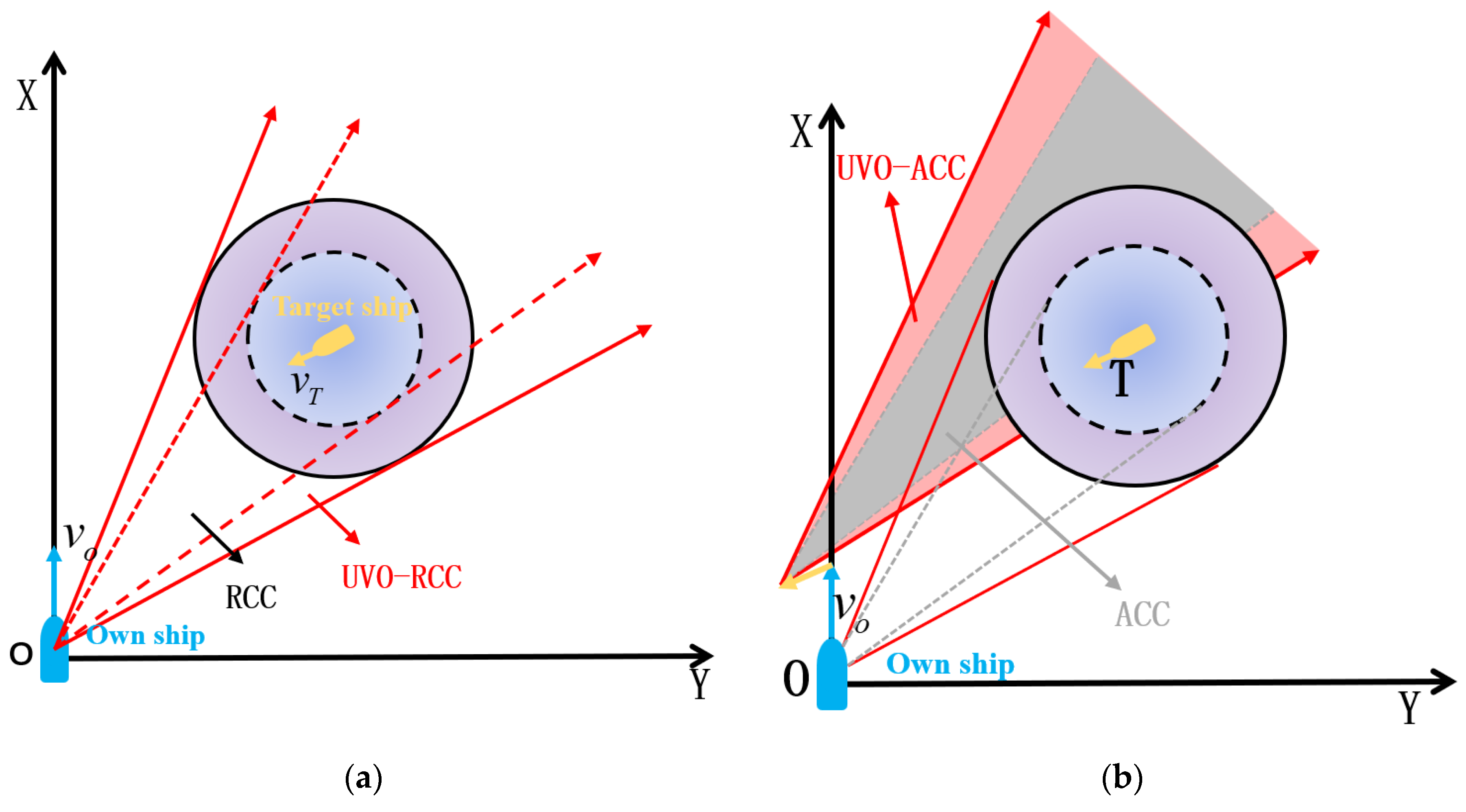
Compared with the baseline deterministic CVaR formulation, the key extension of the present study is that the posterior Gaussian distribution of target vessel position is no longer used only for uncertainty-aware collision-region construction. Instead, it is directly embedded into the loss function of speed optimization. As a result, the velocity-selection problem is transformed from deterministic optimization into stochastic risk-aware optimization under positional uncertainty, enabling the model to explicitly evaluate the tail risk caused by random target-position deviations.

4.2.1. Random Loss Function Construction

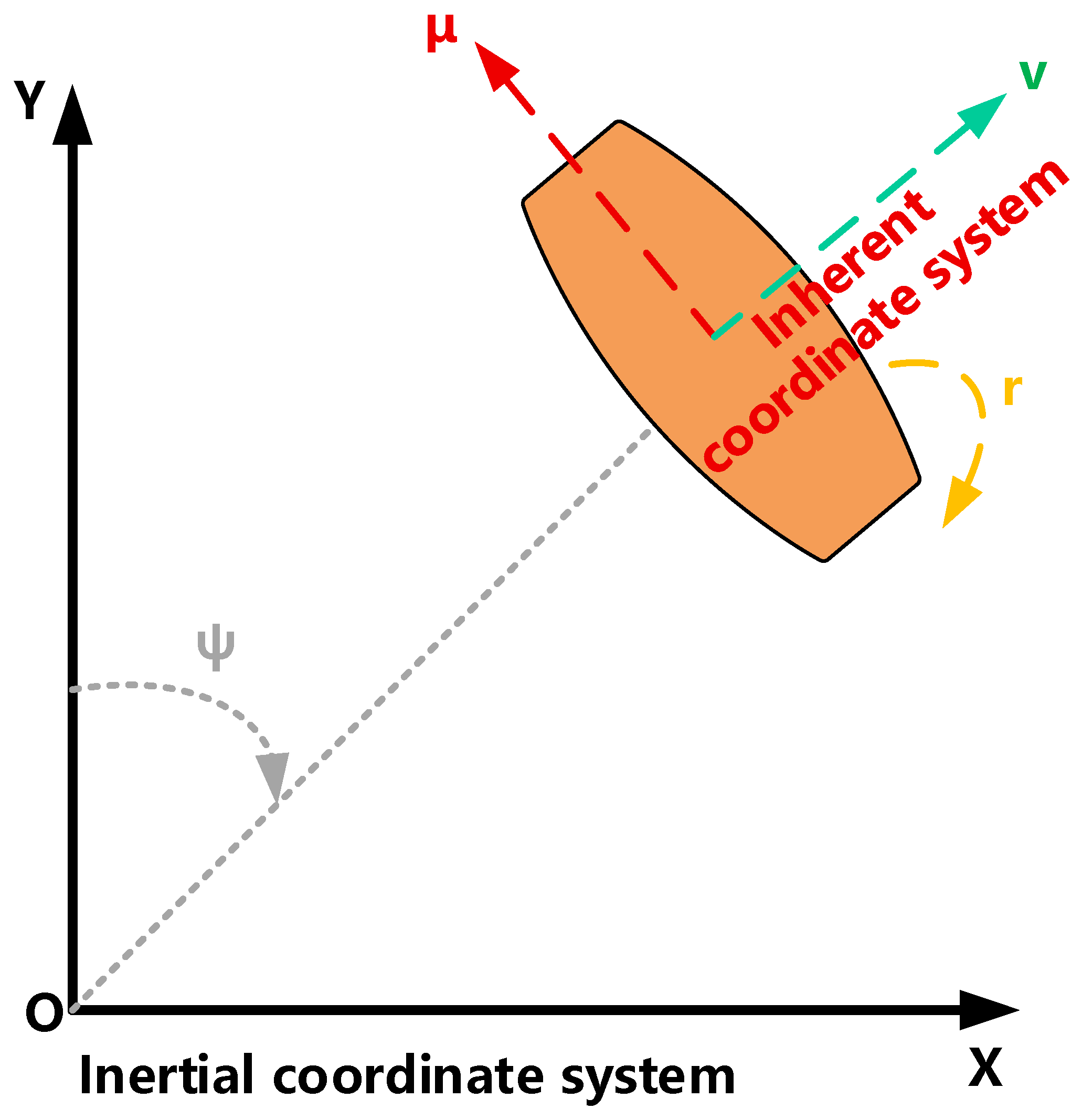
The stochastic loss function is a core component of the improved CVaR model. Its design must simultaneously capture the costs associated with both navigation-efficiency and collision-risk, while embedding the parameters of the uncertain environment as random variables, thereby ensuring that subsequent risk metrics possess clear statistical significance. After introducing uncertainty regarding the target vessel’s position, the nature of the speed selection problem shifts from deterministic optimization to stochastic optimization. Based on the results of Bayesian inference, the position state of the target vessel at time $k$ follows a posterior Gaussian distribution $\mathcal{N}({\hat{X}}_k,P_k)$. Let $\xi$ denote the random variable describing this uncertainty in environmental parameters. For a given candidate velocity vector $v\in V_{\mathrm{adm}}$ (where $V_{\mathrm{adm}}$ is the set of feasible velocities for the home vessel), the total loss function $L(v,\xi )$ is defined as the sum of two components: the navigation efficiency loss $f_{\mathrm{nav}}$ and the collision risk loss $f_{\mathrm{risk}}$:

$$L(v,\xi )=w_1{f}_{\mathrm{nav}}(v)+w_2{f}_{\mathrm{risk}}(v,\xi )$$

(7)

where $w_1$ and $w_2$ are normalized weighting coefficients; by adjusting their ratio, one can flexibly balance efficiency and safety.

• Navigation-efficiency loss is a deterministic term independent of the random realization of the target vessel’s position, consisting of two components: the cost of course deviation and the cost of time delay. The former measures the lateral deviation by calculating the orthogonal projection of the predicted future position onto the original course; the latter measures the time cost incurred by the detour by comparing the difference between the actual path length and the length of the original shortest path. Both cost terms are normalized to ensure dimensional consistency, thereby providing a clear physical interpretation of the weighting coefficients.

This term is intended to quantify the cost of deviating from the planned course when performing an evasion maneuver at speed $v$. It is a deterministic term that does not depend on the stochastic realization of the target vessel’s position. Based on the geometric relationship between the vessel’s current position and the global planned path, the following functional is constructed:

$$f_{\mathrm{nav}}(v)=h_1\cdot {\displaystyle \frac{‖p_{t+\Delta t}\left(v\right)-p_{\mathrm{proj}}‖}{\Delta d_{\max }}}+h_2\cdot {\displaystyle \frac{\Delta t_{\mathrm{delay}}}{\Delta t_{\max }}}$$

(8)

where $p_{t+\Delta t}(v)=p_t+v\cdot \Delta t$ is the predicted position at the next time step; $p_{\mathrm{proj}}$ is the orthogonal projection of $p_{t+\Delta t}$ onto the original flight path; $\Delta t_{\mathrm{delay}}$ is the time delay caused by yaw; $\Delta d_{\max }$ and $\Delta t_{\max }$ are normalization factors; $h_1$ and $h_2$ are weighting coefficients, and satisfy condition $h_1+h_2=1$.

2.

The collision-risk loss is a random variable, and its randomness stems from the Gaussian uncertainty in the target vessel’s position. Within the time window, the minimum encounter distance between the home vessel and the uncertain target vessel depends on the realization of the uncertain environmental parameters. An exponential penalty function is employed: the penalty tends toward zero when the minimum encounter distance is far greater than the safety distance, and increases sharply as the two approach each other. The steepness of the penalty function is controlled by a risk sensitivity factor, enabling a continuous transition from “soft constraints” to “hard constraints.”

This term is a random variable, and its randomness stems from the Gaussian uncertainty in the target vessel’s position. Let $d_{\min }(v,\xi )$ be the minimum Euclidean distance between the home vessel—traveling at speed $v$ within time window $[t,t+\tau ]$—and the uncertain target vessel. An exponential penalty function is used to describe the collision risk:

$$f_{\mathrm{risk}}(v,\xi )=\left\{\begin{array}{ll}\exp \left(\lambda \left(R_{\mathrm{safe}}-d_{\min }(v,\xi )\right)\right),\hfill & \mathrm{if} d_{\min }<R_{\mathrm{safe}}\hfill \\ 0,\hfill & \mathrm{otherwise}\hfill \end{array}\right.$$

(9)

In this context, $R_{\mathrm{safe}}=R_{\mathrm{OS}}+R_{\mathrm{TS}}+{\sigma }_{\mathrm{unc}}$ represents a safety threshold that incorporates uncertainty variance, and it varies with the stochastic realization of the target ship’s position; $\lambda$ is a risk sensitivity factor that controls the steepness of the penalty function.

In this formulation, the deterministic navigation-efficiency term encourages the vessel to maintain a short and smooth route, whereas the stochastic collision-risk term penalizes potentially dangerous velocity choices under positional uncertainty. Their combination allows the proposed method to balance economy and safety in a unified optimization framework.

4.2.2. CVaR-Based Risk Measurement Model

For a given confidence level $\beta \in (0,1)$ (typically 0.95), value at risk is defined as the $\beta$-th percentile of the loss distribution, i.e., the probability that losses will not exceed this value is:

$$Va{R}_{\beta }(v)=\min \{\gamma \in \mathrm{R}:P(L(v,\xi )\le \gamma )\ge \beta \}$$

(10)

However, VaR cannot measure the tail risk beyond the threshold. Therefore, conditional value at risk is introduced, whose physical meaning is the expected loss under the worst-case $(1-\beta )\times 100\%$ scenario:

$$CVa{R}_{\beta }(v)=\mathbb{E}[L(v,\xi )\mid L(v,\xi )\ge Va{R}_{\beta }(v)]$$

(11)

CVaR possesses all the desirable properties of a consistent risk measure, including positive homogeneity, subadditivity, and monotonicity. Furthermore, by introducing auxiliary variables, it can be reformulated as a minimization problem in the following convex optimization framework, thereby greatly facilitating numerical solutions:

$$CVa{R}_{\beta }(v)={\min }_{\gamma \in \mathrm{R}}\left(\gamma +{\displaystyle \frac{1}{1-\beta }}\mathbb{E}\left[{(L(v,\xi )-\gamma )}^{+}\right]\right)$$

(12)

In particular, ${(x)}^{+}=\max (x,0)$. In unmanned vessel collision avoidance scenarios, minimizing CVaR means not only reducing the probability of a collision but also ensuring that, even in the event of extreme positional deviations, the potential losses resulting from a collision are kept to a minimum. This approach is particularly well-suited for unmanned vessel collision avoidance tasks with stringent safety requirements.

Unlike VaR, which only provides a quantile threshold, CVaR characterizes the expected loss in the tail region. Therefore, it is more suitable for USV collision avoidance problems, where a small number of extreme but hazardous target-position deviations may lead to severe consequences.

4.2.3. SAA-Based Speed Optimization Procedure

Because the expectation term in the CVaR reformulation is generally difficult to evaluate analytically, the sample average approximation (SAA) method is adopted. Specifically, the posterior Gaussian distribution of target vessel position is used to generate random disturbance samples, and the expectation in the CVaR objective is approximated by a finite sample average. In this way, the original stochastic optimization problem is transformed into a tractable finite-dimensional optimization problem.

Based on the above analysis, the problem of selecting a robust collision avoidance speed for unmanned vessels is formulated as a speed optimization problem subject to kinematic constraints and COLREG regulations. The optimization objective is to find the optimal velocity vector $v^{*}$ that minimizes the conditional value at risk at a confidence level of $\beta$. The mathematical model is as follows:

$$v^{*}=\arg {\min }_{v\in V_{\mathrm{adm}}}J(v)$$

(13)

$$J(v)=\eta \cdot f_{\mathrm{nav}}(v)+(1-\eta )\cdot CVa{R}_{\beta }\left(f_{\mathrm{risk}}(v,\xi )\right)$$

(14)

Due to the complexity of the analytical solution, the sample mean approximation method is used in practical calculations. Based on the covariance matrix $P_k$, we generate $N$ samples ${\xi }_1,\dots ,{\xi }_N$ of the target vessel’s position; the discrete approximation of the objective function is then:

$$\tilde{J}(v)=\eta \cdot f_{\mathrm{nav}}(v)+(1-\eta )\cdot \left(\gamma +{\displaystyle \frac{1}{N(1-\beta )}}{\displaystyle \sum _{j=1}^N{\left[f_{\mathrm{risk}}(v,{\xi }_j)-\gamma \right]}^{+}}\right)$$

(15)

Constraints:

• Maximum speed constraint: $\Vert v\Vert \le v_{\max }$, ensuring that the selected speed remains within the physical limits of the vessel’s propulsion system.
• Mobility constraints (considering a dynamic window): Taking into account the maximum changes in speed and heading of the unmanned vessel within a finite time step, the set of currently achievable speeds is restricted to a dynamic window centered on the current speed, ensuring that speed commands are physically feasible: $v\in V_{\mathrm{dynamic}}=\{v\mid \Vert v-v_{\mathrm{curr}}\Vert \le a_{\max }\cdot \Delta t\}$.
• Rules and Regulations: The vessel’s course must comply with the COLREG rules for giving way as determined by the current collision situation, including maintaining course and reducing speed in overtaking situations, turning to starboard in head-on situations, and the vessel giving way yielding to the right in crossing situations.

When the sample size $N$ is sufficiently large, the SAA approximate solution converges with high probability to the optimal solution of the true CVaR optimization problem, and the approximation error decreases at a rate of $O\left(1/\sqrt{N}\right)$ as $N$ increases. By adjusting the confidence level $\beta$ and the weight $\eta$, this model can flexibly switch between “aggressive and efficient” and “conservative and safe” driving styles. When uncertainty is high, the CVaR term dominates the optimization process, prompting the unmanned vessel to select a robust speed that keeps it away from regions of uncertainty.

4.3. Integration into the Overall UVO-CVaR Decision-Making Framework

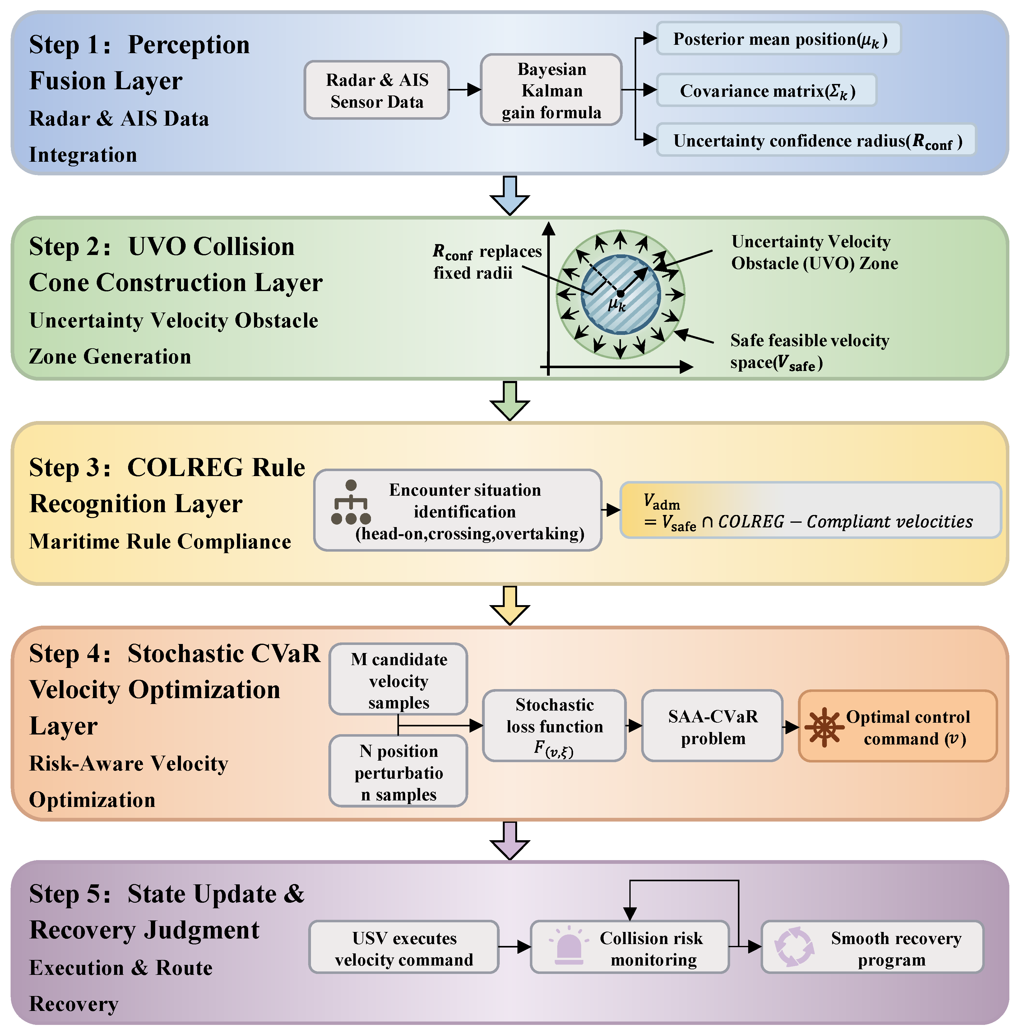
In the overall collision avoidance framework, Steps 1–3 mainly inherit the baseline UVO perception, uncertainty-characterization, and rule-screening pipeline established in previous work, whereas Step 4 constitutes the core methodological extension of the present study. The integrated decision-making framework can therefore be understood as a closed-loop architecture in which the inherited UVO modules provide the uncertainty-aware feasible domain, and the proposed improved stochastic CVaR model performs the final robust speed decision, as shown in Figure 4.

Step 1 (Perception Fusion Layer): In each control cycle, radar polar coordinate measurements and AIS position reports are acquired in real time. The Bayesian Kalman filter is used to perform a posteriori estimation of the target vessel’s position, outputting the posterior mean ${\mu }_k$ and covariance matrix ${\Sigma }_k$. The uncertainty confidence radius $R_{\mathrm{conf}}(t,\alpha )$ is then calculated based on the current confidence level $\alpha$.

Step 2 (UVO Collision Region Construction Layer): Using the posterior mean ${\mu }_k$ as the center of the target vessel’s position and replacing the fixed geometric radius in the traditional velocity barrier method with the confidence radius $R_{\mathrm{conf}}$, construct an absolute collision region $UVO(v_{\mathrm{OS}},v_{\mathrm{TS}},\delta )$ that accounts for positional uncertainty. Determine the velocity barrier region that causes a collision at the current time, and thereby delineate the safe feasible region $V_{\mathrm{safe}}$ in velocity space.

Step 3 (COLREG Rule Recognition Layer): Based on the relative bearing and velocity vector relationship between the vessel and the target vessel, determine the current collision scenario type (overtaking, head-on, or crossing) and the vessel’s duty to avoid a collision (vessel yielding right of way or vessel maintaining course); convert the rule constraints into the velocity-direction feasible region $V_{\mathrm{COLREG}}$, apply directional pruning to $V_{\mathrm{safe}}$, and obtain the constrained velocity set $V_{\mathrm{adm}} = V_{\mathrm{safe}}\cap V_{\mathrm{COLREG}}$ that simultaneously satisfies both safety and compliance requirements.

Step 4 (Random CVaR Speed Optimization Layer): Generate M candidate speed samples from $V_{adm}$ using the dynamic window method; for each candidate speed, sample N position disturbance samples from the Gaussian distribution $N\left({\mu }_k, {\Sigma }_k\right)$, and compute the loss function $F\left(v,{\xi }_n\right)=w_1{f}_{\mathrm{nav}}(v)+w_2{f}_{\mathrm{risk}}(v,\xi )$ for each sample; and solve the SAA-CVaR using the auxiliary variable convexification formula, and select the speed $v$ with the minimum CVaR as the control command output at the current time step.

Step 5 (Status Update and Recovery Decision): The unmanned vessel executes a control step according to $v$ to update its position and heading; it then determines whether it is still within the collision-risk zone. If the risk has been eliminated (i.e., the UVO zones of all target vessels no longer overlap with the vessel’s speed), the system initiates the procedure to resume the original course, smoothly transitioning back to the planned route with the goal of minimizing the deviation distance, thereby completing the entire collision avoidance-recovery closed-loop process.

For implementation clarity, the complete input–output relationship and computational sequence of the proposed UVO-CVaR method are summarized in Algorithm 1.

Algorithm 1. Sequential implementation procedure of the proposed UVO-CVaR method.

Input:

Own-vessel state $\mathrm{OS}$ = {position, heading, velocity}

Radar and AIS observations of target vessels $Z$

Kinematic and dynamic-window constraints $C_{\mathrm{dyn}}$

COLREG rule constraints $C_{\mathrm{COLREG}}$

Confidence level $\alpha$

Number of candidate velocities $\mathrm{M}$

Number of stochastic samples $\mathrm{N}$

Weight coefficients $w$ and $h$

Output:

Optimal collision avoidance velocity command $v*$

Updated own-vessel state $\mathrm{OS}$

1:  Initialize own-vessel state $\mathrm{OS}$ and target vessel observation set $Z$

2:  while collision avoidance task is not completed do

3:      Acquire radar and AIS measurements at current time step

4:      Estimate posterior mean ${\mu }_i$ and covariance ${\sum }_i$ of each target vessel by Bayesian fusion

5:      Compute uncertainty confidence radius $R_{\mathrm{conf},i}$ for each target vessel

6:      Construct UVO region for each target vessel using $\left\{{\mu }_i,{\sum }_i,R_{\mathrm{conf},i}\right\}$

7:      Compute preliminary safe velocity set $V_{\mathrm{safe}}$ by excluding collision-inducing velocities

8:      Identify encounter type according to relative bearing and relative motion

9:      Apply COLREG constraints $C_{\mathrm{COLREG}}$$\mathrm{to} V_{\mathrm{safe}}$$\mathrm{and} \mathrm{obtain} \mathrm{constrained} \mathrm{set} V_{\mathrm{c}}$

10:     Generate $\mathrm{M}$$\mathrm{candidate} \mathrm{velocities} \left\{v_{\mathrm{m}}\right\}$$\mathrm{from} V_{\mathrm{c}}$ using the dynamic window method

11:     for each candidate velocity $v_{\mathrm{m}}$ do

12:         Draw $\mathrm{N}$$\mathrm{disturbance} \mathrm{samples} \left\{{\xi }_{\mathrm{n}}\right\}$ from the posterior Gaussian distribution

13:         for each sample ${\xi }_{\mathrm{n}}$ do

14:             Evaluate navigation-efficiency loss $f_{\mathrm{nav}}(v_{\mathrm{m}})$

15:             Evaluate collision-risk loss $f_{\mathrm{risk}}(v,{\xi }_{\mathrm{n}})$

16:             Compute total stochastic loss $L(v,\xi )$

17:         end for

18:         Compute SAA-based CVaR estimate of candidate velocity $v_{\mathrm{m}}$

19:     end for

20:     Select the candidate velocity with minimum CVaR as $v*$

21:     Execute $v*$ and update own-vessel state $\mathrm{OS}$

22:     if all target vessels are cleared from the collision-risk region then

23:         Initiate route-recovery maneuver

24:     end if

25:  end while

26:  return $v*$$, \mathrm{OS}$

5. A Velocity-Selection Model Based on an Improved CVaR Method

Vessel collision avoidance can be divided into four stages: identifying the risk of collision with another vessel, taking evasive action in accordance with the Rules of the Road, resuming the original course, and stabilizing the vessel on its original route. To verify the effectiveness of the collision avoidance algorithm proposed in this study, simulation analysis was conducted using MATLAB 2023b, with the experimental scenario involving multiple-vessel encounters in open, complex waters. The home vessel and the approaching vessel were modeled as circular shapes based on their actual dimensions. In the multi-ship collision avoidance experiments, simulation experiments were conducted using the UNLVO method described in Reference [21], the traditional UVO-CVaR method described in Reference [22], and the improved UVO-CVaR method described in this study.

5.1. Multi-Vessel Collision Avoidance Scenario 1

The initial parameters for the Multi-Vessel Collision Avoidance Scenario 1 simulation are shown in

Table 2. Table of vessel parameters for Experiment 1: Multi-Vessel Collision Avoidance Scenario.

Ship Parameters	Own Vessel	Target Vessel 1	Target Vessel 2	Target Vessel 3	Target Vessel 4
Length (m)	4.88	4.88	10	4.88	10
Width (m)	2.5	2.5	5	2.5	5
Initial x- Coordinate (m)	0	30	150	350	450
Initial y- Coordinate (m)	0	0	−100	50	−100
Initial heading Angle (°)	90	90	148	247	284
Initial velocity (m/s)	2	0.2	1	0.8	0.8

.

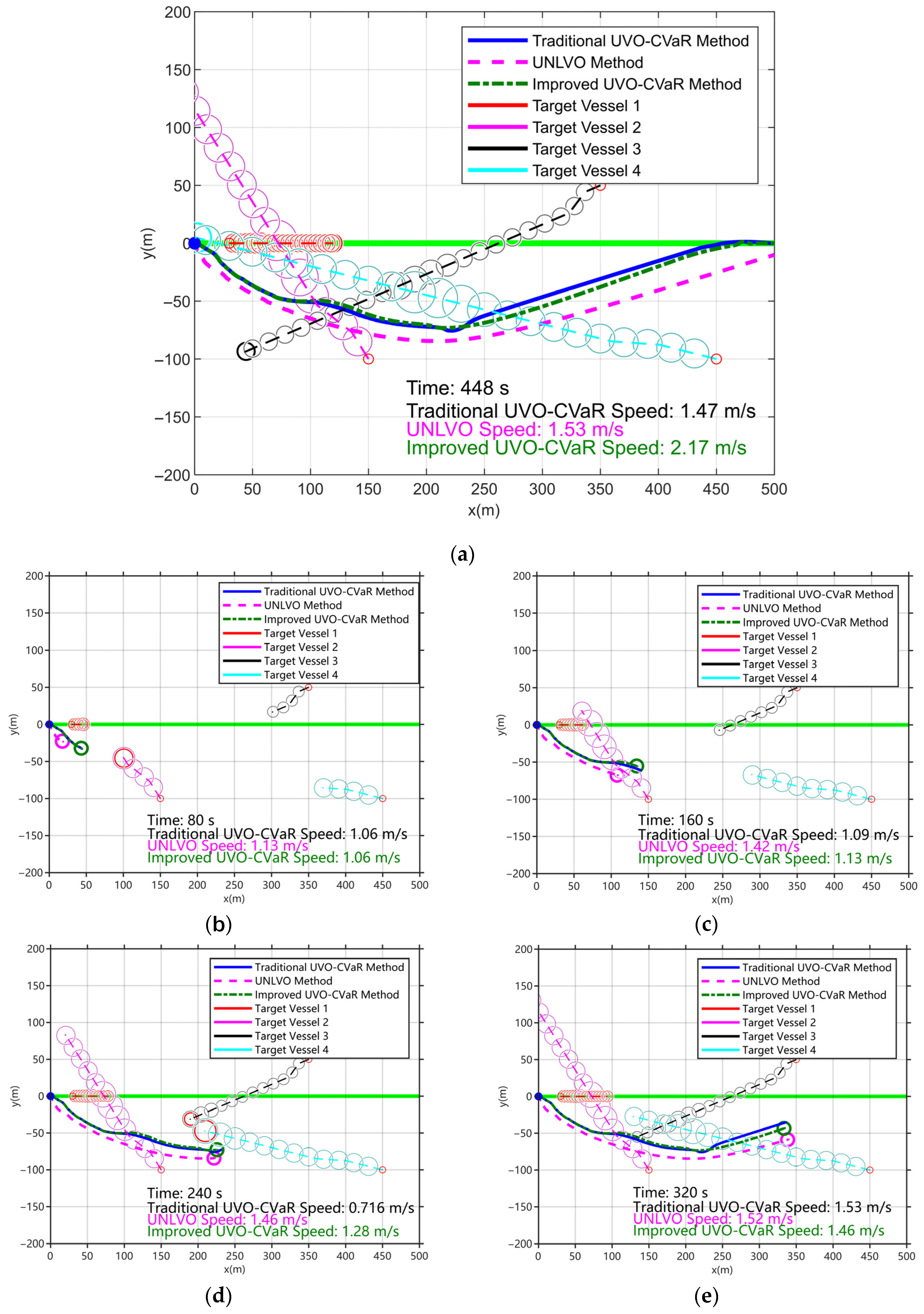
In Multi-Vessel Collision Avoidance Scenario 1, Target Vessel 1 is a vessel traveling from west to east. Target Vessel 2 has an initial heading of 148°; at the 20 s mark, it turns 20° to port, and at the 70 s mark, it returns to its original heading. Target Vessel 3 has an initial heading of 247°; at the 20 s mark, it turns 30° to port, and at the 50 s mark, it returns to its original heading. Target Vessel 4 has an initial heading of 284°; at the 50 s mark, it turns 10° to port, and at the 90 s mark, it returns to its original heading.

As shown in Figure 5, when using the UNLVO method described in Reference [21], the vessel is capable of performing multi-vessel collision avoidance tasks. However, since the UNLVO method calculates the information for all target vessels in the scene simultaneously and directly selects a speed that avoids all target vessels, the system has limited ability to handle uncertainties in the positions of target vessels when faced with intersecting multi-vessel scenarios. Consequently, the collision avoidance paths exhibit some redundancy, resulting in suboptimal overall navigation efficiency.

When using the traditional UVO-CVaR method described in Reference [22], the vessel’s collision avoidance system sequentially detects collision risks with various target vessels during navigation and gradually implements evasive maneuvers, ultimately completing the collision avoidance task and returning to its original course. However, since the collision avoidance trajectory was not optimized, the vessel’s overall navigation path is relatively long, the magnitude of course adjustments during the avoidance process is significant, and the economic efficiency is relatively poor.

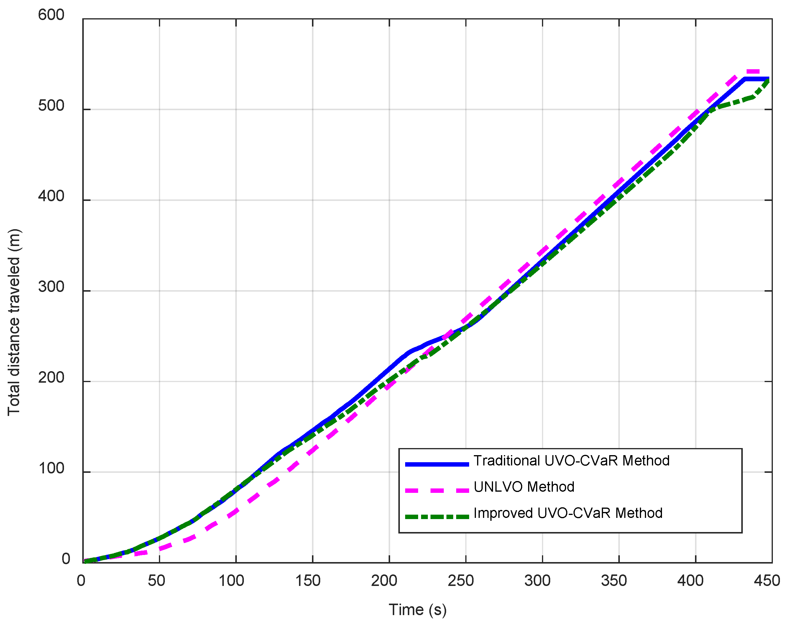
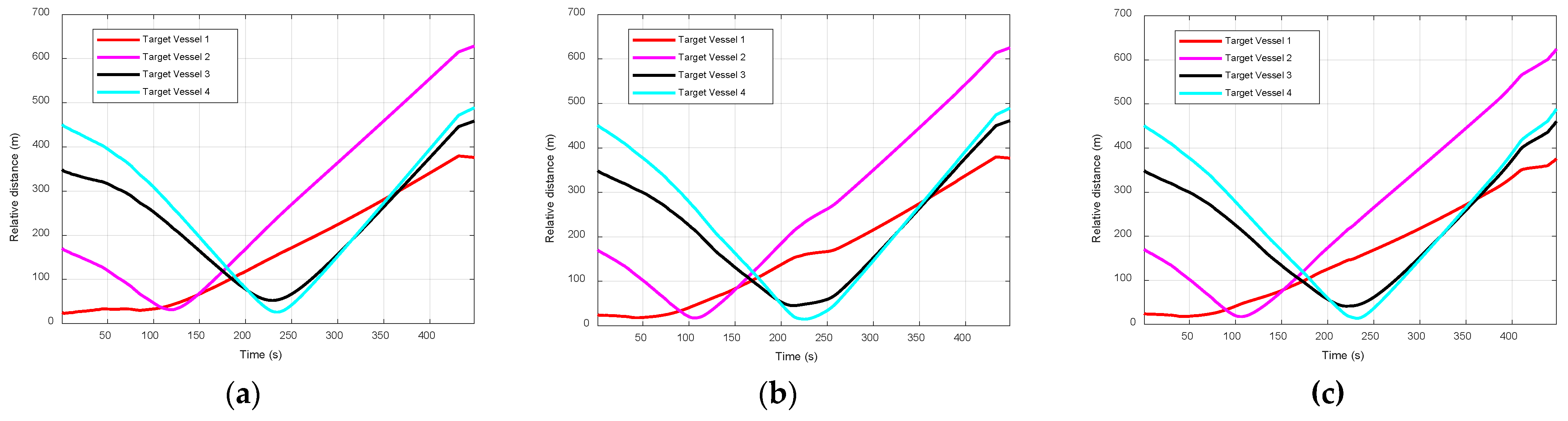
In Multi-Vessel Collision Avoidance Scenario 1, all three methods successfully completed the collision avoidance task. As shown by the experimental data in Figure 6 and Figure 7 and

Table 3. Table of experimental data for the Multi-Ship Collision Avoidance Scenario 1 using the UNLVO method in Reference [21], the UVO-CVaR method in Reference [22], and the improved UVO-CVaR method.

Title 1	Title 2	UNLVO Method	UVO-CVaR Method	Improved UVO-CVaR Method
The closest approach distance between this vessel and the target vessel (m)	Target Vessel 1	24.03	18.55	18.55
	Target Vessel 2	33.11	19.65	19.60
	Target Vessel 3	53.56	46.07	44.40
	Target Vessel 4	28.28	14.32	16.85
Total path length (m)		544.04	529.49	522.61
Runtime of the collision avoidance algorithm (s)		448	440	422

, the UNLVO method calculates the motion information of all target vessels in the scene simultaneously and directly selects a speed that avoids all threats. Consequently, the collision avoidance path exhibits some redundancy in multi-target intersection scenarios. The total path length is 544.04 m, and the algorithm runs for 448 s, resulting in relatively low overall navigation efficiency. Although the traditional UVO-CVaR method can sequentially detect collision threats and gradually implement evasive maneuvers to ultimately complete the collision avoidance task and resume the original course, the overall navigation path is relatively long at 529.49 m due to the lack of path optimization. The method involves significant course adjustments during the avoidance process, resulting in relatively poor economic efficiency, with an algorithm runtime of 440 s. Upon detecting a collision hazard, the improved UVO-CVaR method employs a trajectory optimization strategy to effectively reduce the total navigation path length to 522.61 m and minimize unnecessary heading adjustments, all while ensuring safety. The algorithm execution time is reduced to 422 s. This method demonstrates the best performance in both path economy and algorithm execution efficiency, validating the effectiveness of the proposed improved method in conventional multi-vessel collision avoidance scenarios.

5.2. Multi-Vessel Collision Avoidance Scenario 2

The initial parameters for the Multi-Vessel Collision Avoidance Scenario 2 simulation are shown in

Table 4. Table of vessel parameters for Experiment 2: Multi-Vessel Collision Avoidance Scenario.

Ship Parameters	Own Vessel	Target Vessel 1	Target Vessel 2	Target Vessel 3	Target Vessel 4
Length (m)	4.88	4.88	10	4.88	10
Width (m)	2.5	2.5	5	2.5	5
Initial x- coordinate (m)	0	100	175	300	300
Initial y- coordinate (m)	0	−75	−100	−100	110
Initial heading angle (°)	90	0	0	290	223
Initial velocity (m/s)	2	1.5	0.8	1.17	1.76

.

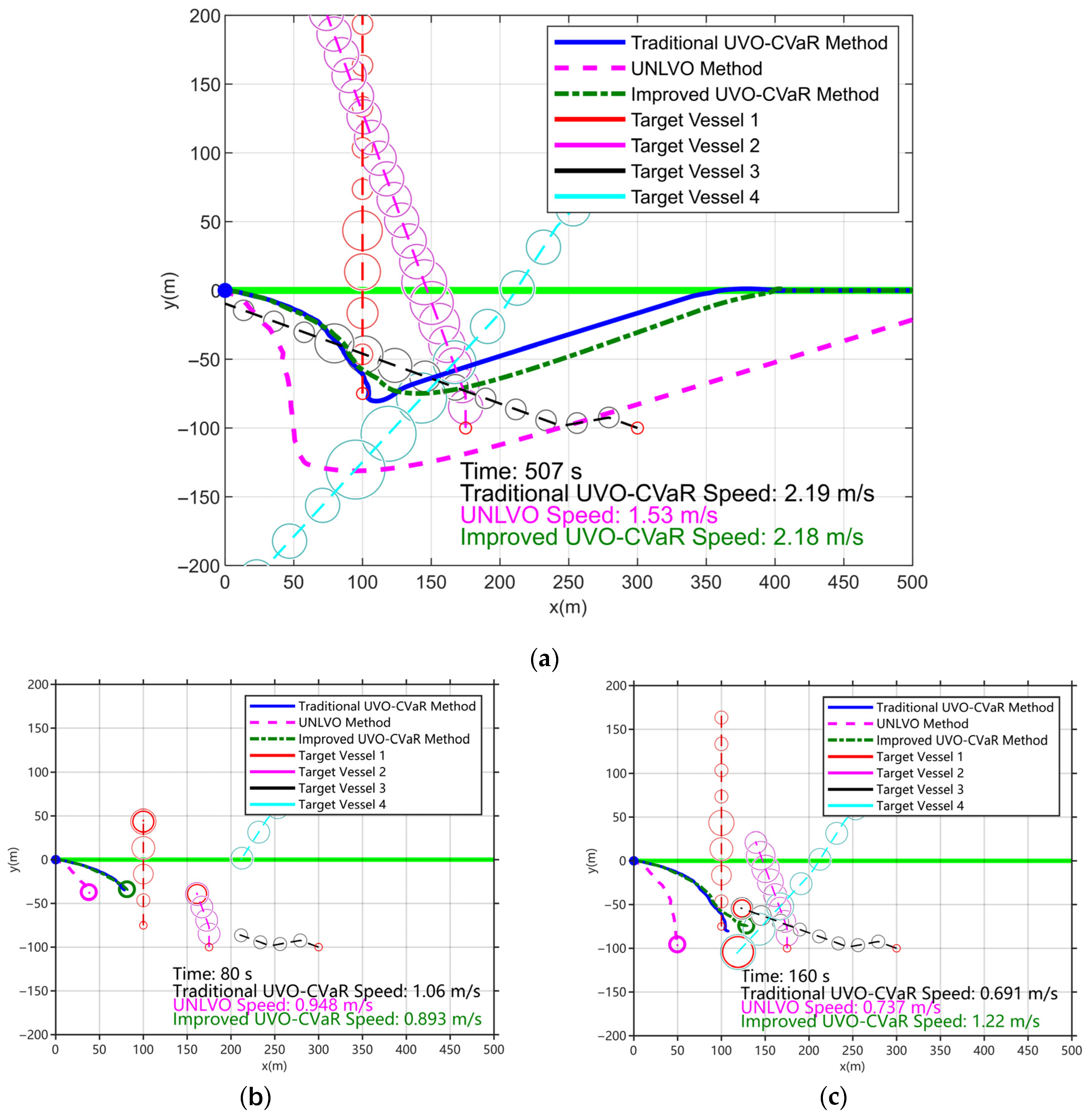
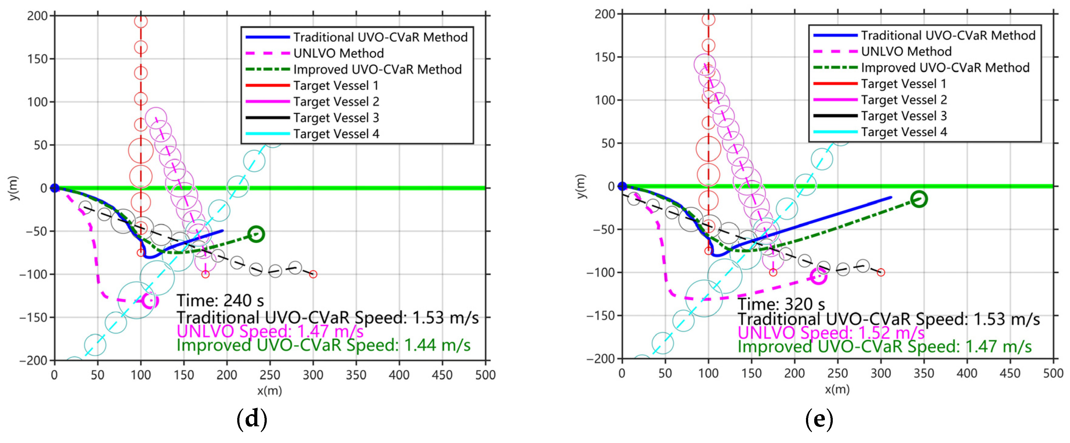
In Multi-Vessel Collision Avoidance Scenario 2, as shown in Figure 8, Target Vessel 1 is a vessel traveling from south to north. Target Vessel 2 has an initial heading of 0°, and at 300 s, it turns 20° to the left. Target Vessel 3 has an initial heading of 290°. At the 20 s mark, it turns 30° to port, and at the 50 s mark, it returns to its original heading. Target Vessel 4 has an initial heading of 223°. At the 50 s mark, it turns 10° to port, and at the 90 s mark, it returns to its original heading.

As shown in Figure 8, when using the UNLVO method described in Reference [21], the home vessel was unable to determine a safe speed at the start and began at a very slow speed; it only began to accelerate once the target vessel had reached a safe speed at a certain point in time. Due to the characteristics of the UNLVO method, although it can accomplish multi-vessel collision avoidance tasks, the turning angles are often excessive, resulting in a significant amount of redundancy in the collision avoidance path. This leads to an overly long total collision avoidance path and insufficient overall navigation efficiency.

When using the traditional UVO-CVaR method described in Reference [22], after this vessel gave way to Target Vessel 1, it approached a collision risk with Target Vessel 3 and also faced a collision risk with Target Vessel 4. Consequently, it turned right to avoid the collision and reduced speed, even resulting in a situation where it was sailing in the same direction as Target Vessel 3. Because Target Vessel 3 was traveling at a relatively high speed, once Target Vessel 3 had passed our vessel, our vessel began to turn toward the destination. The collision avoidance path obtained using the traditional UVO-CVaR method was the longest involved behavior that clearly violated the rules.

When using the improved UVO-CVaR method, the collision avoidance system is able to effectively implement correct collision avoidance strategies that comply with the Rules of the Road upon detecting a collision risk, and the collision avoidance algorithm can determine a safe speed for avoidance. Once all target vessels have passed the point of right of way, the vessel promptly adjusts its course to resume sailing along its original route.

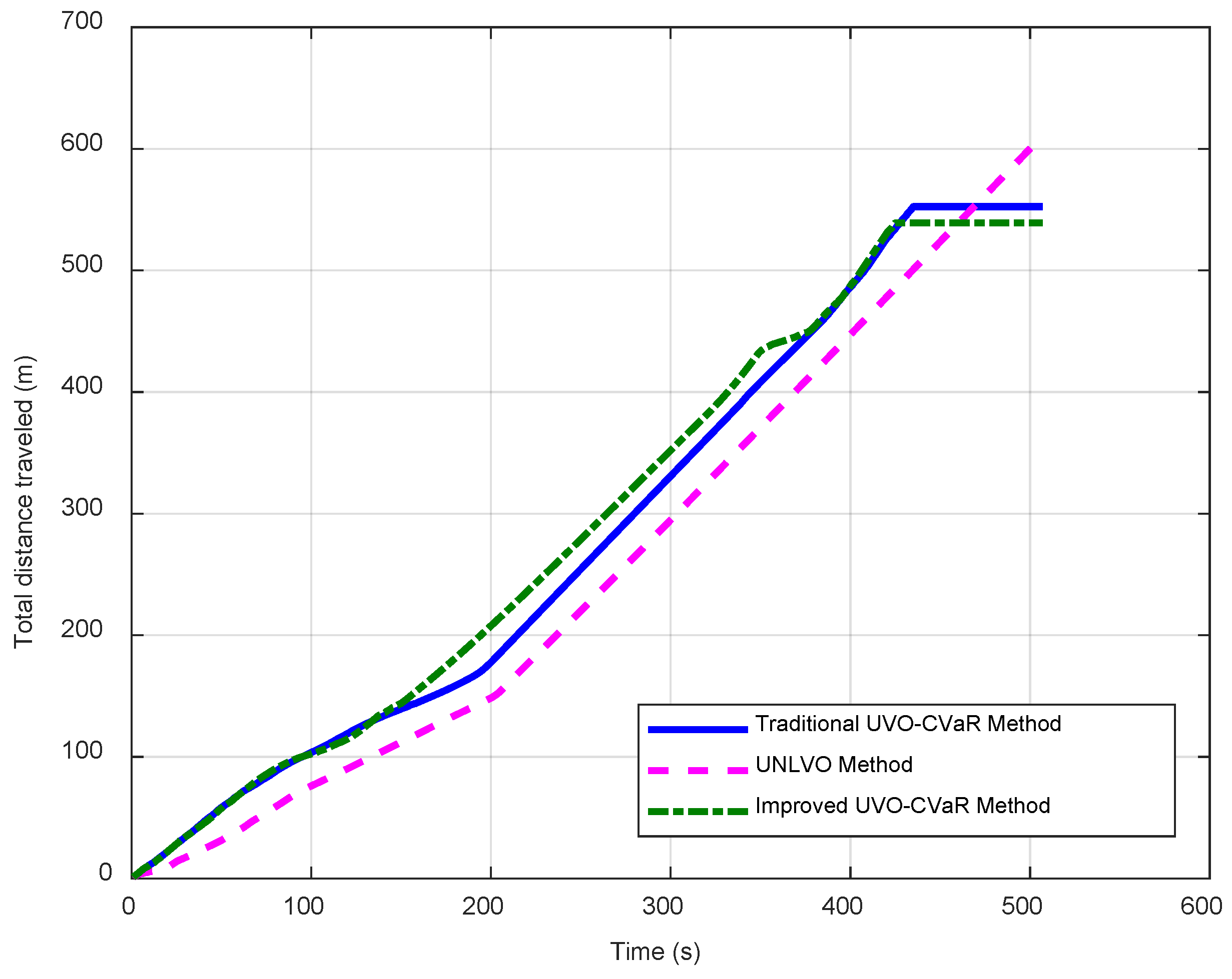
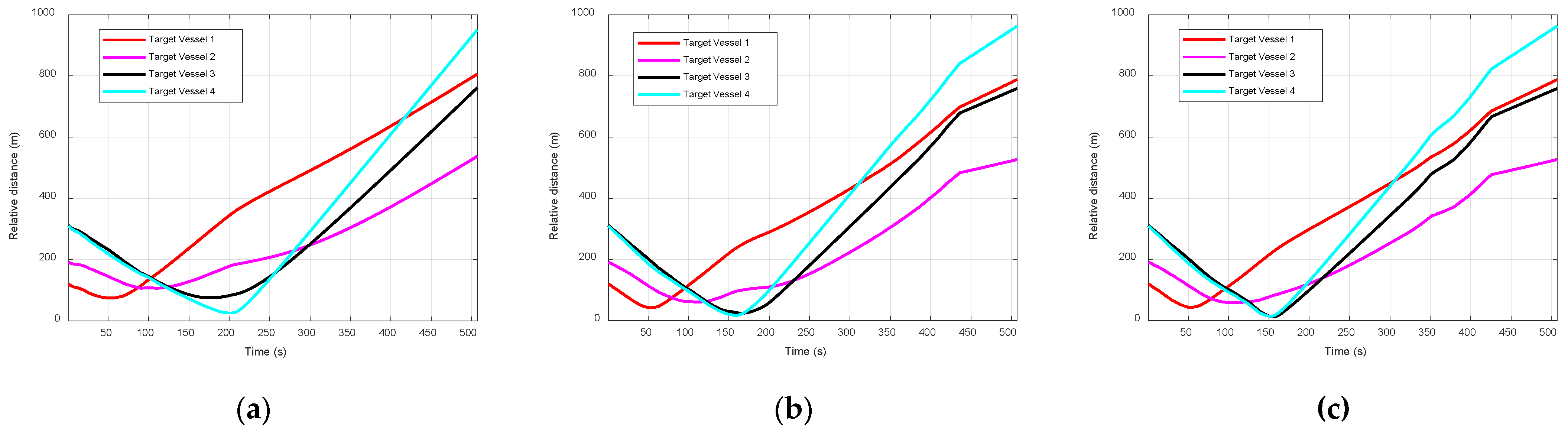
Multi-Vessel Collision Avoidance Scenario 2 is more complex than Scenario 1 in terms of the number of target vessels, their motion patterns, and dynamic maneuvering behavior, further highlighting the performance differences among the three methods. As shown in the experimental data in Figure 9 and Figure 10 and

Table 5. Table of experimental data for the Multi-Ship Collision Avoidance Scenario 2 using the UNLVO method in Reference [21], the UVO-CVaR method in Reference [22], and the improved UVO-CVaR method.

Title 1	Title 2	UNLVO Method	UVO-CVaR Method	Improved UVO-CVaR Method
The closest approach distance between this vessel and the target vessel (m)	Target Vessel 1	75.79	43.86	45.01
	Target Vessel 2	107.47	61.36	59.46
	Target Vessel 3	76.32	15.74	19.15
	Target vessel 4	27.41	19.15	17.17
Total path length (m)		609.30	552.46	539.27
Runtime of the collision avoidance algorithm (s)		506	435	425

, the UNLVO method exhibited an extremely low initial speed during the early stages of the simulation because it could not find a speed that satisfied the safety constraints; it only gradually accelerated after the target vessels moved to a position where a safe speed became available. At the same time, due to the inherent characteristics of the method, the overall steering angle was relatively large, resulting in significant path redundancy. The total path length was 609.30 m, and the algorithm runtime was 506 s. After avoiding Target Vessel 1, the traditional UVO-CVaR method exhibited abnormal behavior—a sharp right turn and significant deceleration—when facing collision threats from Target Vessels 3 and 4. It even began to follow Target Vessel 3 in the same direction, constituting maneuvering that clearly violates the rules. Only after Vessel 3 had passed did the test vessel turn toward the destination, resulting in a total path length of 552.46 m—the longest among the three methods—with an algorithm runtime of 435 s. The improved UVO-CVaR method can still accurately identify collision hazards and adopt correct, compliant evasion strategies in complex multi-vessel dynamic scenarios. After all target vessels have been cleared, the vessel quickly resumes its original course. The total path length is 539.27 m, and the algorithm runtime is 425 s. Both key metrics outperform the other two methods, fully validating the robustness and engineering practicality of the proposed method in complex scenarios.

Through comparative simulation experiments of Multi-Vessel Collision Avoidance Scenarios 1 and 2, this study systematically evaluated the collision avoidance performance of the UNLVO method from Reference [21], the traditional UVO-CVaR method from Reference [22], and the improved UVO-CVaR method across three dimensions: total path length, algorithm runtime, and closest encounter distance. The experimental results indicate that all three methods successfully completed the collision avoidance task in Scenario 1; however, their performance diverged more significantly under the complex dynamic multi-vessel crossing conditions presented in Scenario 2. Due to limitations in its uncertainty handling mechanism, the UNLVO method exhibited high path redundancy and relatively low overall navigation efficiency in complex multi-object scenarios. The traditional UVO-CVaR method exhibits significant yaw deviations and even non-compliant maneuvers when facing specific crossing scenarios, resulting in the poorest path economy. The improved UVO-CVaR method, by introducing a trajectory optimization mechanism, achieves the shortest total path length and the shortest algorithm runtime in both experimental scenarios, while maintaining safe encounter distances with all target vessels, and its collision avoidance decision-making process complies with the basic requirements of the “Rules.” Overall, the proposed improved method achieves significant enhancements over existing methods in terms of safety, economy, and compliance, providing a reliable theoretical basis and technical support for autonomous collision avoidance path planning of unmanned surface vessels in complex sea conditions.

The superior performance of the improved UVO-CVaR method stems from two aspects. First, by incorporating posterior positional uncertainty into the risk evaluation process, the method can avoid selecting velocities that appear safe under deterministic assumptions but become hazardous under stochastic deviations. Second, the CVaR-based objective emphasizes tail-risk control, allowing the vessel to maintain safer and more regulation-compliant maneuvers in complex multi-vessel encounters while still preserving route economy.

6. Discussion

This study addresses the problem of multi-vessel collision avoidance path optimization for USVs in uncertain marine environments. It proposes a UVO-CVaR collision avoidance decision-making framework based on an improved CVaR method. The main contributions and discussions are as follows.

(1)

A foundational collision avoidance framework that integrates uncertainty modeling with the velocity obstacle method is established. First, a three-degree-of-freedom kinematic model for unmanned vessels is developed, and a representation framework for the absolute collision region is constructed based on the velocity obstacle method, providing theoretical support for subsequent decision-making. Second, the uncertainty in the target vessel’s position is modeled as a Gaussian distribution. By fusing multi-source sensor data from radar and AIS through Bayesian inference, the posterior position estimate is dynamically updated, leading to the development of the UVO method. This effectively extends the capability of the traditional velocity obstacle method to handle random errors in the target vessel’s position.

(2)

A stochastic speed optimization method that balances navigation efficiency and tail-end collision risk is proposed and validated. Building on the deterministic CVaR speed selection framework, the Gaussian posterior distribution of the target vessel’s position derived from Bayesian fusion is directly embedded into the loss function, formulating a stochastic optimization model that is efficiently solved using the sample mean approximation (SAA) method. This approach enhances the robustness of speed decisions against positional deviations while strictly adhering to COLREG regulations. The effectiveness of the proposed UVO-CVaR method is systematically verified through two sets of multi-vessel collision avoidance simulation experiments. The results demonstrate that the method outperforms both the UNLVO method and the traditional UVO-CVaR method in terms of total path length and algorithm runtime. Moreover, it is capable of generating correct and compliant collision avoidance strategies even in complex dynamic multi-vessel crossing scenarios, achieving optimal overall performance.

The proposed method still has certain limitations: as the number of target vessels increases further, the impact of the SAA sampling size on computational efficiency requires further evaluation. Future research will aim to validate the adaptability of the proposed method in higher-density traffic scenarios and under complex meteorological conditions, and explore hybrid collision avoidance decision-making architectures that integrate data-driven methods such as reinforcement learning, in order to further enhance the autonomous collision avoidance capabilities of unmanned surface vessels in real-world complex sea conditions.