Article

Baroclinic Semidiurnal Tidal Currents over the Head of the Biobio Canyon, Central Chile


by
Marcus Sobarzo
1,2,
Piero Mardones
3 and
Gonzalo S. Saldías
2,4,*
1
Departamento de Oceanografía, Universidad de Concepción, Concepción 4070386, Chile
2
Centro de Investigación Oceanográfica COPAS Coastal, Universidad de Concepción, Concepción 4070386, Chile
3
Centro de Investigación en Ecosistemas de la Patagonia (CIEP), Coyhaique 5951601, Chile
4
Departamento de Física, Facultad de Ciencias, Universidad del Bío-Bío, Concepción 4051381, Chile
*
Author to whom correspondence should be addressed.
J. Mar. Sci. Eng. 2026, 14(9), 811; https://doi.org/10.3390/jmse14090811
Submission received: 1 April 2026 / Revised: 23 April 2026 / Accepted: 24 April 2026 / Published: 28 April 2026
(This article belongs to the Section Physical Oceanography)

Abstract

This study characterizes the structure and variability of baroclinic semidiurnal tidal currents at the head of the Biobio Submarine Canyon (BbC), off central Chile, based on Acoustic Doppler Current Profiler (ADCP) and moored thermistor-chain observations from two deployments conducted in 2013 and 2014 under contrasting stratification conditions. The results show that the head of the BbC is a dynamically active site of semidiurnal variability, with markedly stronger and more coherent baroclinic motions during the more stratified winter–spring 2014 period. During that deployment, semidiurnal baroclinic current amplitudes reached up to 17 cm s−1, and the associated energy was concentrated near the surface and bottom. Rotary spectral analysis indicated that these semidiurnal baroclinic currents rotated anticyclonically and were closely aligned with the canyon axis. Empirical orthogonal function (EOF) analysis further showed that their vertical structure was dominated by a first baroclinic mode, which explained more than 70% of the semidiurnal baroclinic variance in 2014. In contrast, the 2013 deployment exhibited weaker and less coherent semidiurnal baroclinic variability. Taken together, these results indicate that stronger stratification favored the development of semidiurnal internal-tide-related motions over the canyon head and that the BbC provides a dynamically favorable setting for enhanced semidiurnal internal-tide activity and potentially elevated mixing, although direct turbulence or dissipation measurements were not available in this study. These findings have potential implications for local water-column structure, nutrient supply, and primary productivity in this highly productive coastal region.

1. Introduction

Submarine canyons are deep, steep-sided, and relatively narrow submerged valleys typically characterized by V-shaped isobaths [1]. They are prevalent features on continental shelves worldwide [2], serving as important conduits for sediment transport from coastal regions to the deep ocean. In the California Current System, approximately 20% of the continental shelf between Alaska and the Equator is interrupted by submarine canyons, with some areas exhibiting interruptions of up to 50% [3]. The submarine canyons play a crucial role in regional coastal ecosystems, fostering areas of high biodiversity and enhanced biological productivity [2,3,4,5,6].
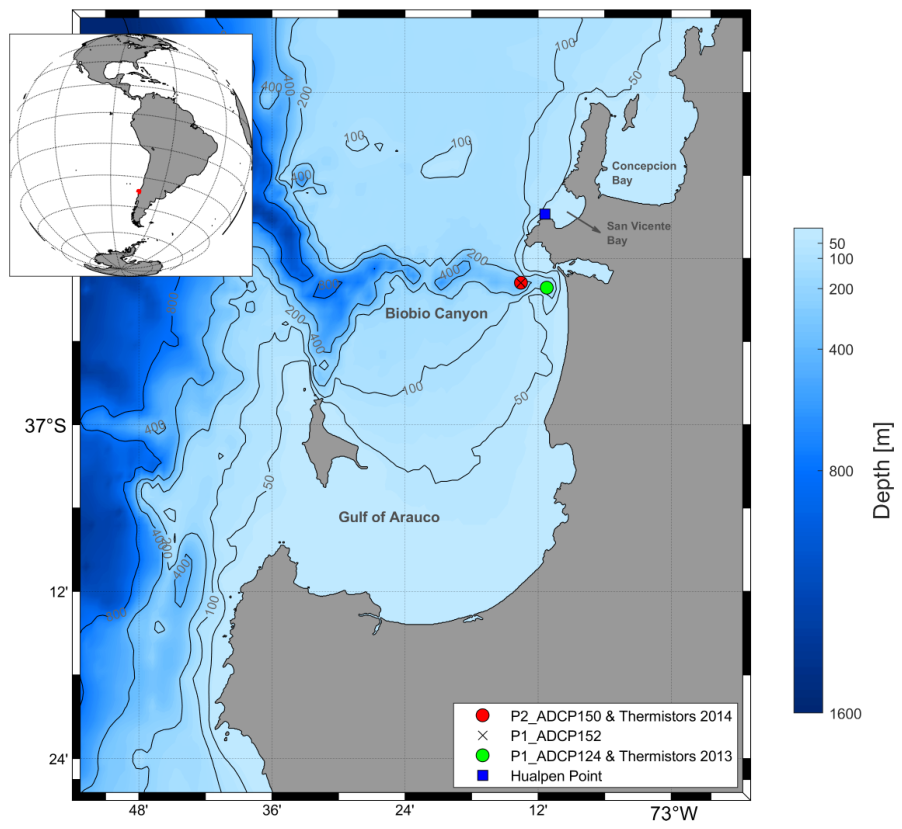
At least 11 submarine canyons are found along the continental shelf off central-south Chile between 33° S and 40° S [7]. The Biobio Submarine Canyon (BbC) is located at the northern end of the Gulf of Arauco (36°49′ S) and extends from the mouth of the Biobio River to the ocean trench, reaching a depth of approximately 4570 m [8] and separating the Gulf of Arauco from the continental shelf north of the BbC (Figure 1). Due to its dimensions (length and depth), the BbC is one of the longest canyons in Chile, measuring approximately 100 km. Its head is about 300 m from the coast. Compared to other coastal areas, the Gulf of Arauco and the adjacent coastal zone are among the most biologically productive regions in the southeastern Pacific [9].
Coastal upwelling and biological productivity in submarine canyons can be enhanced by locally forced topographic upwelling, driven by a pressure gradient oriented perpendicular to the coast and parallel to the canyon axis [4,10]. On the continental shelf, currents that flow along the coast are geostrophically balanced by a pressure gradient perpendicular to the coast. However, inside the canyon, the alongshore velocity is abruptly reduced, and the pressure gradient perpendicular to the coast extends vertically, penetrating the canyon and generating an acceleration of the flow along its zonal axis, thereby promoting the onshore transport of deep waters [11,12].
In addition, the turbulent mixing generated by the breaking of internal waves also plays a vital role in regions with irregular coastal topography [13,14,15]. In this context, submarine canyons are particularly important, as they are recognized as sites of internal wave generation and modification, with fluctuations that are often larger than those observed in the open ocean [16,17,18,19,20,21]. In general, submarine canyons can intensify the energy of tidal and internal waves by trapping waves propagating from the open ocean [22] or by locally generating energy, as these regions frequently exhibit critical slopes [16]. Based on observational data, Kunze et al. [13] proposed that the small-scale roughness of the Monterey Submarine Canyon is responsible for a significant portion of internal tidal energy dissipation.
Despite the recognized importance of submarine canyons in generating internal waves and enhancing turbulent mixing, few studies have been conducted in Chile. Research on submarine canyons along the Chilean coast has focused mainly on geological aspects, particularly related to sediment transport and deposition [7,8,23,24]. Other observational studies [10,25,26] and modeling studies [27] have described the influence of BbC on coastal subinertial flows, on the ecology of the intertidal zone [28], and on the effects of internal tides on slope currents [29]. Aguirre et al. [30] analyzed the semidiurnal tidal currents offshore central Chile (36.6° S) during the winter and summer of 2005. Their results showed that internal semidiurnal currents were dominant in the San Vicente and Concepción bays, exhibiting counterclockwise rotation throughout the water column and larger amplitudes during winter, which were associated with stronger stratification. Similarly, Bravo et al. [31] analyzed the semidiurnal tidal currents (barotropic and baroclinic) in two upwelling regions, Coquimbo (30° S) and Concepción (36°30′ S). They observed significant variability in semidiurnal baroclinic currents during summer in Coquimbo and during winter in Concepción, both periods coinciding with stronger stratification. Both studies highlighted the potential importance of the BbC as a significant source of internal tides.
In this study, we use current, temperature, sea-level, and wind observations collected at the head of the Biobio Canyon during two deployments in 2013 and 2014 to characterize the structure and variability of semidiurnal tidal currents under contrasting stratification conditions. Specifically, we examine the vertical structure of the total, barotropic, and baroclinic currents; their spectral and harmonic characteristics, including tidal ellipses and rotary behavior; and the dominant vertical modes of semidiurnal baroclinic variability through EOF analysis. By comparing both periods, we assess how stratification and canyon geometry modulate the intensity and structure of internal-tide-related motions over the canyon head.

2. Data and Methods

Observations and Data Processing

Time series of hourly-averaged currents, sea level, and temperature were collected at the head of the BbC during two periods: November to December 2013 (P1) and August to October 2014 (P2). Additional wind data was also recorded from a nearby meteorological station (Figure 1). High-resolution bathymetry (approximately 5 m) was provided by Jara-Muñoz et al. [32] and prepared by González-Acuña and Arroyo-Suarez [33].
During P1, two 300 kHz RDI Workhorse Acoustic Doppler Current Profilers (ADCPs; Teledyne RD Instruments, CA, USA) were moored at depths of 152 and 124 m on the head of the BbC, hereafter referred to as P1_ADCP152 and P1_ADCP124, respectively. These instruments recorded current data every 10 min for 31 days (P1_ADCP152) and 38 days (P1_ADCP124). The vertical resolution was 6 m and 2 m, respectively. In addition, the ADCPs provided bottom-temperature and bottom-pressure measurements. Two chains of thermistors were deployed near ADCPs, each equipped with 6 HOBO (Onset Computer Corporation, MA, USA) temperature sensors distributed throughout the water column (Table 1). However, only the thermistor chain installed near P1_ADCP124 was recovered. Near P1_ADCP152, hydrographic profiles were collected at regular intervals for 48 h, using an SBE25 CTD-O (Sea-Bird Scientific, WA, USA) between November 11 and 13. These profiles provided temperature, salinity, density, pressure, and oxygen data during that period.
During P2, a 300 kHz RDI Workhorse ADCP with a vertical resolution of 6 m was deployed at the same location (P2_ADCP150), with a sampling interval similar to that of the P1_ADCP152 deployment. A thermistor chain equipped with 7 HOBO temperature sensors was also installed. In addition, hydrographic profiles were collected using an SBE25 CTD-O at 11 stations along the main axis and the edges of the canyon on September 11, 2014 (Table 1). During both periods, the data was complemented with measurements of the magnitude and direction of the wind from a meteorological station located on the Hualpén peninsula (blue box, Figure 1).
Because the three ADCP deployments did not sample the water column identically, and the near-surface and near-bottom layers were not fully resolved in all cases, the vertical-average estimate of the barotropic current and the resulting baroclinic residual may contain some uncertainty, particularly when comparing deployments with different depth coverage and vertical resolution.
A spectral analysis was performed on the sea-level data obtained from the ADCP pressure sensor by dividing the series into three segments, yielding 6 degrees of freedom [34]. This choice represents a compromise between variance reduction and frequency resolution, while still retaining sufficient resolution to identify the dominant diurnal and semidiurnal energy peaks. As a result, lower-frequency variability, such as the fortnightly band, is not well resolved. In addition, a tidal harmonic analysis was conducted using the same data to determine the amplitude and phase associated with each tidal constituent [35]. The tidal regime within the canyon was characterized using the form factor F = ( K 1 + O 1 ) / ( M 2 + S 2 ) , where the numerator and denominator correspond to the amplitudes of the diurnal and semidiurnal constituents, respectively. According to the standard classification, F < 0.25 indicates a semidiurnal regime, 0.25 F < 1.5 a mixed regime with semidiurnal dominance, 1.5 F < 3 a mixed regime with diurnal dominance, and F 3 a diurnal regime.
The barotropic current was estimated as the vertical average of the velocity profiles, considering that the measurements covered nearly the entire water column [30,31,36]. The baroclinic component was calculated by subtracting the barotropic component from the total current at each depth level. Subsequently, a tidal harmonic analysis was performed on barotropic and baroclinic currents to determine the parameters of the tidal ellipses for each tidal component.
Rotary autospectra were computed by dividing each time series into three non-overlapping Hanning-tapered segments ( k = 3 ), yielding an estimator with ν = 2 k = 6 effective degrees of freedom (EDOF). Following Emery and Thomson [34], this gives a 95% confidence interval of [ 0.38 , + 0.69 ] in log 10 units, which is a constant additive range independent of frequency. Statistical significance of spectral peaks was evaluated against a red-noise AR(1) background spectrum fitted independently at each depth level. Peaks exceeding this depth-dependent background by a factor χ 2 ( ν , 0.95 ) / ν 2.10 are significant at the 95% level [37].
The current and temperature series were filtered using a 221-weight Lanczos band-pass cosine filter with cut-off periods of 9–15 h to isolate variability around the semidiurnal band. This filter allows less than 7% of the variability to leak outside the selected frequency band [31]. Empirical orthogonal function (EOF) analysis was applied to baroclinic current components (zonal and meridional) to examine the dominant vertical oscillation modes associated with semidiurnal variability [34]. The 9–15 h Lanczos band-pass filter was applied to isolate semidiurnal variability broadly rather than to separate individual semidiurnal constituents. Specific constituent identification and ellipse parameters were instead obtained from the tidal harmonic analysis of the original series. Accordingly, the band-pass-filtered variability may include nearby semidiurnal constituents such as N2, M2, and S2.

3. Results

3.1. Wind, Sea Level, and Temperature

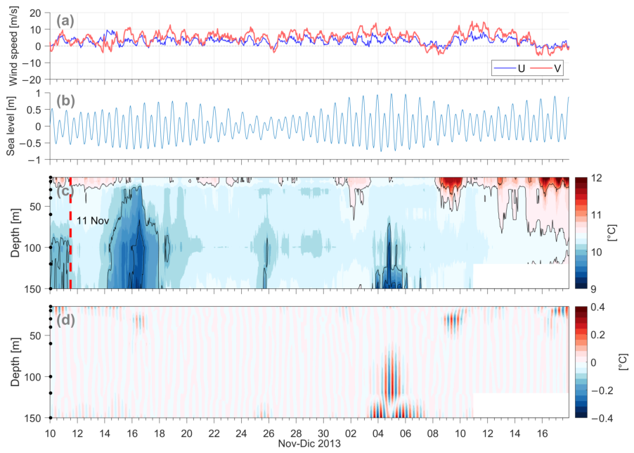
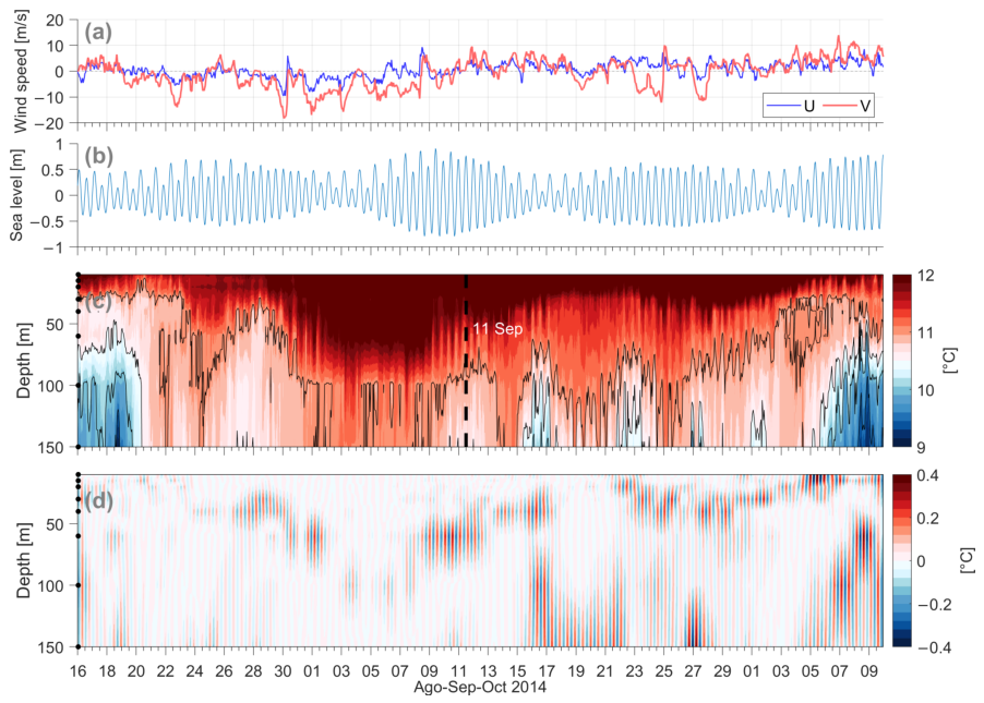
During P1, the wind along the coast (component v) showed a predominant northward direction with daily fluctuations reaching maximum speeds of approximately 14 m/s. Southward wind events were less frequent, with two significant events recorded in December (Figure 2a). Wind variability was highest at the diurnal frequency, primarily in the zonal component, and was associated with a sea breeze regime typical of the southern spring–summer period. During winter and spring 2014 (P2), the wind exhibited greater variability, particularly in its v-component, due to the frequent passage of low-pressure systems that generated a southward component (Figure 3a). The strongest southward winds occurred between 30 August and 7 September, reaching a maximum magnitude of ∼19 m/s (Figure 3a).
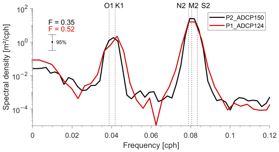
The sea level spectra of both periods of study exhibited maximum energy around the diurnal and semidiurnal frequency bands, indicating a predominantly semidiurnal mixed tidal regime (Figure 4). Due to the short duration of the time series, the fortnightly signal was not visible in the spectra. Harmonic analysis of sea level indicated that the most important astronomical constituent during both periods was the M 2 tide, with an amplitude close to 44 cm. This was followed in amplitude by the K 1 constituent during P1 and by the S 2 constituent during P2, with amplitudes of ∼19 cm. The form factor (F) was 0.52 and 0.35 for P1 and P2, respectively.
In this tidal regime, the semidiurnal temperature fluctuations intensified with the increase in thermal stratification generated by solar surface heating and subsurface cooling associated with topographic upwelling (Figure 2c and Figure 3c). During P1, a predominantly well-mixed water column was observed, except for some subsurface topographic upwelling events [10] and surface heating toward the end of the period. During these subsurface cooling events, the semidiurnal frequency fluctuations reached magnitudes of approximately ± 0.4  °C (Figure 2d). In contrast, during P2, corresponding to a winter–spring period, a much more stratified water column was observed, with stratification becoming even more pronounced during certain subsurface cooling events (Figure 3c). During this time of year, a more stratified water column favored the development of high-frequency thermal fluctuations (Figure 3d). The difference between the two periods was notable, as, unlike during P1, these fluctuations were observed throughout nearly the entire measurement period in 2014.
Furthermore, maximum shoaling of cold waters (below 10 °C) was associated with the coupling between a coastal trapped wave and the spring tide, as previously documented for this period by Sobarzo et al. [10]. This contrast is particularly evident when comparing the elevation of cold waters during the first subsurface cooling event (which occurred during neap tides) and the last event (during spring tides) of P2 (Figure 3b,c).
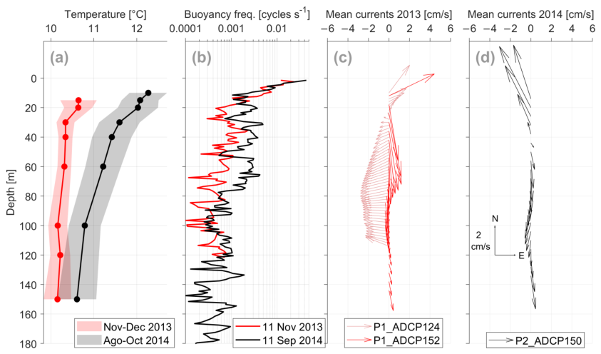
To complement the above, the average temperature profiles from the thermistors during both periods revealed contrasting vertical structures. During P1, the average profile was nearly uniform, with an average temperature of 10.35  °C and a standard deviation of 0.25  °C, with slightly warmer temperatures at the surface than at the bottom. In contrast, the 2014 cruise exhibited a more pronounced vertical gradient, with average temperatures around 12.5  °C near the surface and 10.5  °C near the bottom (standard deviation ± 0.4  °C) (Figure 5a). Subsurface cooling events tended to increase temperature variability, as reflected in higher standard deviations near the bottom in both cruises. The buoyancy frequency profiles derived from the selected CTD-O cast further confirmed the greater vertical stratification observed in 2014 (Figure 5b). However, these profiles represent only a specific time and do not capture all of the temporal variability over the study period.
The favorable coastal upwelling winds during P1 led to a colder, more vertically mixed water column than P2. In contrast, the thermal stratification observed during winter 2014 was mainly driven by subsurface cooling associated with topographic upwelling, rather than surface heating from solar radiation.

3.2. Total and Baroclinic Currents at the Head of the Biobio Submarine Canyon

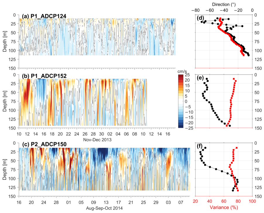
The total hourly current data for the three current meters (two P1 and one P2) was decomposed along their respective major principal axes (MPAs). During P1, the currents along the MPAs were weaker at the head of the canyon (124 m) compared to the more oceanic site (152 m) (Figure 6a,b). These lower current intensities were likely associated with the local geometric configuration of the canyon head, where the 124 m mooring occupied a more protected position relative to the 152 m mooring (Figure 1). In P1_ADCP124, the percentage of explained variance was less than 60% in the upper 40 m of the water column. However, below 50 m depth, the explained variance increased to more than 80%, indicating that the MPA estimates were more robust at depth and reflected more elliptical current patterns. Additionally, below 50 m, the orientation of MPA tended to align more zonally, coinciding with the canyon’s main axis (0°, indicating eastward) (Figure 6e). For P1_ADCP152 and P2_ADCP150, the percentage of explained variance fluctuated between 60 and 80%, and the direction of MPA became increasingly diagonally aligned with the canyon axis with depth (Figure 6c). These results indicate that the predominant current direction tended to become more zonally aligned with increasing depth, particularly in the more coastal ADCP deployment.
During P1, the average flow recorded by P1_ADCP124, closest to the coast, indicated a northeastward flow (coastward) with mean velocities of approximately 2.5 cm/s to a depth of ∼20 m (Figure 5c). Below this depth, the mean flow was predominantly westward, out of the canyon, with average velocities also ∼2.0 cm/s. The ADCP positioned farther offshore (P1_ADCP152) recorded a strong northeastward mean flow near the surface, with velocities reaching ∼4 cm/s, a predominantly southward flow below 20 m. This southward flow was most intense near 30 m depth (approximately 4.5 cm/s), gradually decreasing with depth until reaching velocities close to 1 cm/s at 144 m. During the 2014 cruise, the mean flow in the upper 40 m was directed northwestward, with velocities around 5 cm/s, higher in intensity than those observed during the previous campaign (Figure 5d). Below 40 m, the flow was predominantly southward.
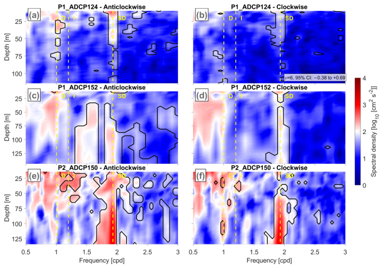
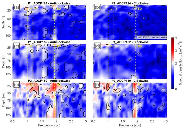
The rotational spectra of the total currents revealed significant energy concentrated in the semidiurnal and diurnal bands (Figure 7), with the highest energy densities observed at P2_ADCP150. The modest number of effective degrees of freedom ( ν = 6 ) associated with our record length yields a 95% confidence interval that spans roughly one order of magnitude in log 10 , which accounts for the broadband variance visible between the main tidal peaks, including oscillations near the inertial and lower frequencies. The semidiurnal anticlockwise peak exceeds the 95% significance level (solid black contour) over a substantial fraction of the water column at P2_ADCP150, confirming that this feature is robust. Wind forcing may also contribute to the observed diurnal variability, particularly near the surface, since the sea breeze displayed peak energy within the diurnal band and was more intense during P1. When comparing the two cruises, the energy around the semidiurnal band was nearly an order of magnitude higher during P2 (Figure 7e,f), a difference that clearly exceeds the 95% CI and is therefore robust.
During P1, the variance associated with baroclinic currents was concentrated near the surface (Figure 8a–d), with patches exceeding the 95% significance level along the semidiurnal band particularly in the anticlockwise component. In contrast, at P2_ADCP150 the baroclinic variance showed well-defined maxima around the semidiurnal band, both near the bottom and at the surface (Figure 8e,f), with a broader region exceeding the 95% significance contour. Energy was also present around the near-inertial and diurnal bands.
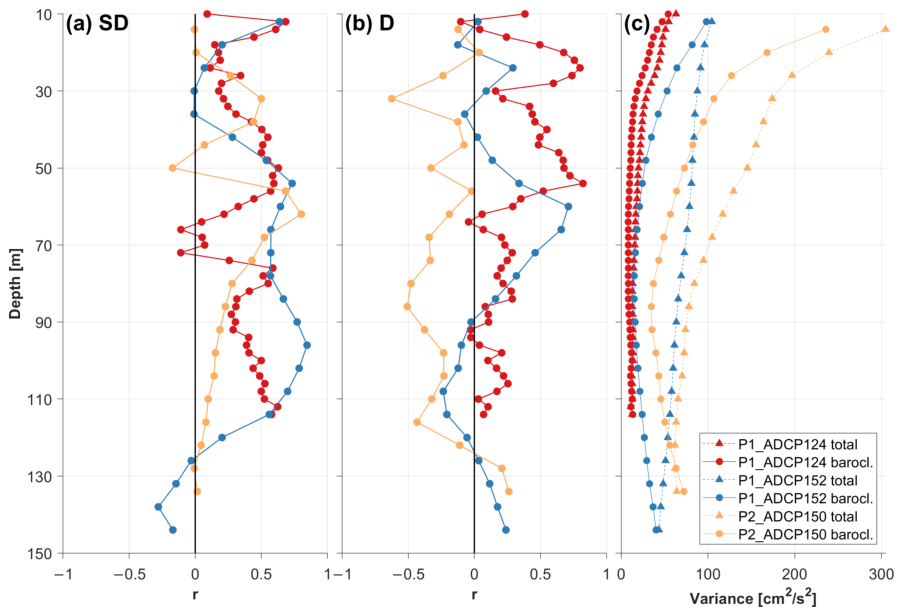
During both study periods, the rotation coefficient of the semidiurnal baroclinic currents was positive throughout nearly the entire water column (Figure 9a), indicating an anticlockwise rotation (anticyclonic in the southern hemisphere). This supports the interpretation that the energy observed in this frequency band may be associated with internal waves, which exhibit exclusively anticyclonic rotation [38]. In contrast, the diurnal band exhibited more pronounced differences between ADCPs. In particular, P2_ADCP150 showed a predominantly clockwise rotation throughout most of the water column (Figure 9b).
In general, the variance profiles of the total current were greater than those of the baroclinic component in both periods (Figure 9c). The highest energy levels were observed in P2_ADCP150, while the lowest were recorded at P1_ADCP124. However, the pattern of the percentage of variance explained by baroclinic currents relative to total variance was similar across all deployments. In all cases, the highest explained variances (>80%) occurred near the surface and the bottom. In contrast, a minimum in baroclinic variance was consistently observed around the middle of the water column, approximately between 40 and 90 m depth. This mid-depth minimum is consistent with the nodal depth of the first baroclinic mode (60–80 m), which implies weaker baroclinic motions in the middle of the water column and stronger amplitudes near the surface and bottom; near-bottom amplification may also be favored by interaction with canyon topography.

3.3. Barotropic and Baroclinic Semidiurnal Currents

The ellipses of the barotropic semidiurnal currents showed an orientation more or less parallel to the main axis of the canyon, particularly during the winter and spring of 2014, when the ellipse showed its highest amplitude and was well aligned with the central axis of the canyon in the zonal direction (Figure 10).
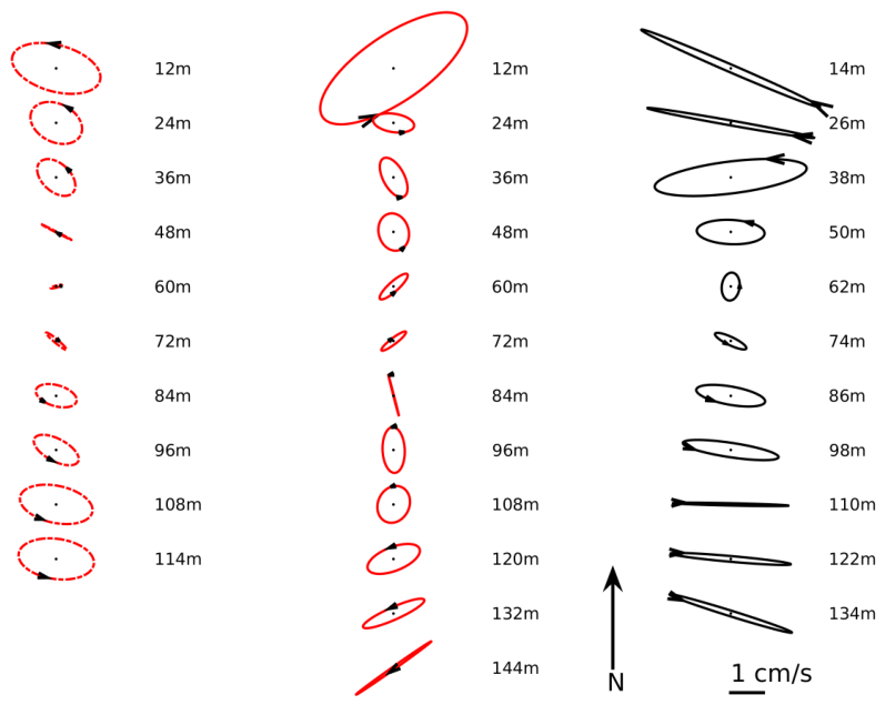
In the case of the ellipses of the semidiurnal baroclinic current, all were notably small in the mid water column, around 60 m depth, and more pronounced near the surface and bottom (Figure 11). A key feature observed during P2 was the high ellipticity, particularly near the bottom and the surface, suggesting oscillatory motions with minimal rotation and aligned with the canyon axis. In contrast, the ellipses were smaller and more circular during P1, indicating weaker baroclinic current fluctuations, characterized by greater rotational motion and less evident alignment with the canyon axis.
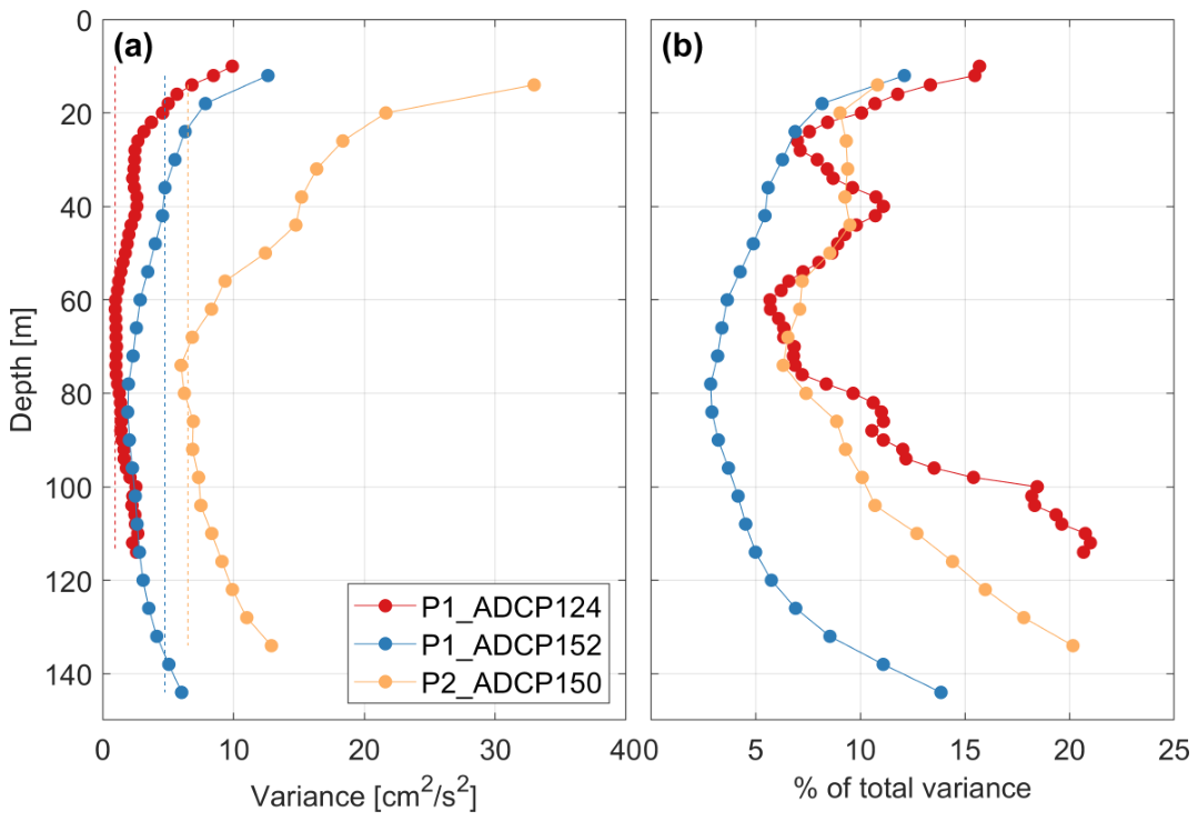
The vertical structure of the variance of the semidiurnal baroclinic currents consistently showed greater baroclinic than barotropic variance near the surface and bottom (Figure 12a), consistent with the variance patterns previously observed in the unfiltered baroclinic currents (Figure 9c). In particular, the variance of the semidiurnal baroclinic currents in P2_ADCP150 was elevated throughout the water column, with values ranging from 6 to 33 cm2/s2. The variance of the baroclinic currents was also relatively high throughout the water column for P1_ADCP124. However, the values generally remained below 5 cm2/s2 except in the upper 20 m, where this threshold was exceeded. In contrast, the weakest semidiurnal baroclinic signal was between 40 m depth and near the bottom, with a comparatively higher contribution from the semidiurnal barotropic component (∼5 cm2/s2) in P1_ADCP152. In terms of the percentage of the total current variance (Figure 12b), semidiurnal baroclinic currents represented 5–20% in most cases. An exception was P1_ADCP152, where values below 5% were observed between 40 and 120 m depth. In all deployments, the maximum percentage of baroclinic variance occurred near the bottom (up to 20%, except at P2_ADCP150), followed by a secondary maximum near the surface, with values between 10% and 15%.
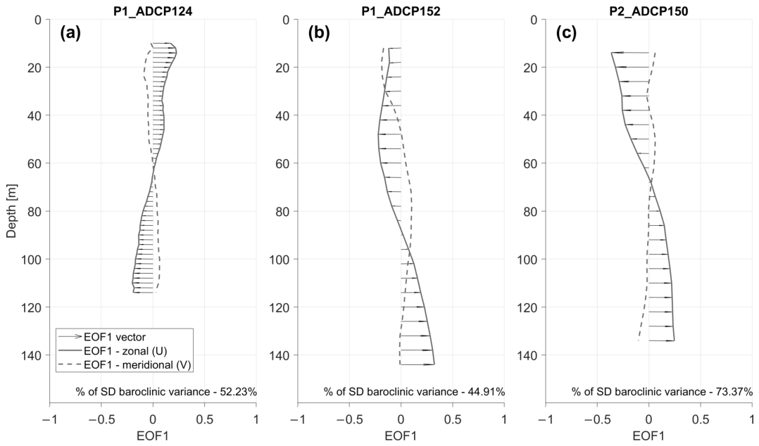
The first empirical orthogonal function mode of the baroclinic semidiurnal currents exhibited a similar vertical structure, with a predominantly zonal orientation and a nodal depth between 60 and 80 m (Figure 13a–c). This first mode can be interpreted as the first baroclinic mode of an internal wave aligned with the canyon’s central axis (the zonal component). The first mode explained 52.2% and 44.9% of the variance at P1_ADCP152 and P1_ADCP124, respectively. In contrast, the first mode was more clearly defined during P2, accounting for 73.4% of the variance, suggesting a stronger and more coherent baroclinic structure than during the 2013 deployment.

4. Discussion

4.1. Canyon Influence on High-Frequency Currents

The rotary spectra of both total and baroclinic currents showed elevated variance not only at the diurnal and semidiurnal peaks, but also across the frequencies between them, producing broader and less sharply defined spectral peaks than those previously reported for the adjacent continental shelf. In contrast, previous studies conducted on the continental shelf off Concepcion have reported spectra with distinct peaks at these tidal frequencies [30,31]. The elevated energy outside these bands observed in our study may be influenced by the Biobio Canyon (BbC), which could alter tidal frequencies and current dynamics. Wavelet analysis of near-bottom currents from P2_ADCP150 revealed a redistribution of energy around the semidiurnal band to longer periods on certain days. In particular, diurnal tidal amplification has also been documented in the Gully Submarine Canyon, Canada [39]. In addition, near-inertial oscillations have been detected on the continental shelf adjacent to the BbC and may propagate into the canyon [40]. The canyon’s topographic complexity could further modify the frequency of these oscillations by altering potential vorticity through depth variations along the canyon axis.
The semidiurnal baroclinic fluctuations observed at the head of the BbC were notably more intense than those reported in previous studies on the adjacent continental shelf. The peak velocities reached up to 17 cm/s—nearly twice the maximum values recorded by Aguirre et al. [30] and Bravo et al. [31] during summer and winter 2005 and 2009, respectively. These high velocities were observed despite comparable or even stronger stratification than in our measurements (Figure 5b), with buoyancy frequencies (N) ∼0.01 cps over the continental shelf [30] and ∼ 5 × 10 4 cps at a station farther north (36.51 °S) [31]. These findings support the interpretation that the BbC may serve as a site of internal wave generation [30,31]. This interpretation is further reinforced by the variance of the semidiurnal baroclinic currents observed during the 2014 mooring, which exceeded 20 cm2/s2 at the canyon head, more than twice the values reported for other shelf sites and for San Vicente Bay, where the variance remained below 10 cm2/s2 [30].
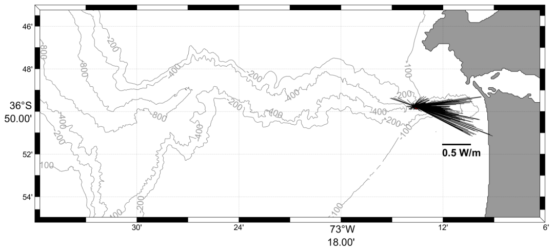
The results revealed a dominant first EOF mode of semidiurnal baroclinic currents, associated with the first baroclinic mode of the internal wave structure, which is consistent with previous findings [30,31]. In both of those studies, this first mode accounted for no more than 60% of the total variance of the semidiurnal baroclinic currents. In contrast, during the most stratified period of our study (2014), this mode explained 73% of the total variance within the BbC. Additionally, the total variance of the semidiurnal baroclinic currents during 2014 was significantly higher than in the aforementioned studies, indicating that this first mode was much more energetic than previously observed in nearby areas of the continental shelf. Another relevant finding is that, in the BbC, particularly during P2 (2014), the tidal currents were strongly aligned with the canyon axis. This behavior contrasts with observations from many other submarine canyons worldwide, where tidal currents tend to cross the canyon axis or flow parallel to the continental shelf break. Examples include Hydrograph Canyon [22], Hudson Canyon [16], Monterey Canyon [13,18,19], La Línea Canyon [41], and Gaoping Canyon [42]. The alignment of the barotropic tide with the canyon axis appears to be a key factor in explaining the high energy observed in semidiurnal baroclinic fluctuations within the BbC and their influence on nearby continental shelf dynamics. This pattern is further supported by the vector diagram of the semidiurnal energy flux associated with the first dynamic mode during P2, which shows that the energy was predominantly directed along the canyon axis (Figure 14).

4.2. Implications of Vertical Mixing Associated with Internal Tides in Submarine Canyons

Turbulent mixing is a fundamental long-term process that maintains thermohaline circulation [43]. It can alter the stratification of the water column and regulate short-term variability in nutrient concentrations within a given region [44]. In this context, understanding the physical processes that drive mixing is essential for assessing their impact on primary productivity on temporal scales ranging from hours to days.
In coastal regions, mixing processes require mechanical energy input, which can be supplied by wind forcing, tidal motions, or freshwater discharge [45]. In the Gulf of Arauco, the high productivity observed has been attributed to coastal upwelling, a key feature of eastern boundary current systems [46,47]. This upwelling exhibits seasonal and synoptic-scale variability (3 to 15 days), largely modulated by fluctuations in alongshore wind intensity. However, as previously noted, high-frequency turbulent mixing also plays a crucial role in shaping physical and biogeochemical dynamics in coastal zones.
Internal tides play a crucial role as intermediaries in converting barotropic tidal energy into turbulent mixing. Egbert and Ray [48] estimated that the global dissipation of semidiurnal tidal energy (M2) in the open ocean amounts to approximately 700 GW. In contrast, estimates of global internal tidal dissipation would range from 200 GW [49] to 360 GW [50]. Based on the higher end of this estimate, Carter and Gregg [51] suggested that submarine canyons contribute approximately 15% of global semidiurnal internal tidal dissipation (M2), corresponding to about 58 GW. Using numerical simulations, Jachec et al. [52] calculated a dissipation rate of approximately 8.3 MW for Monterey Canyon.
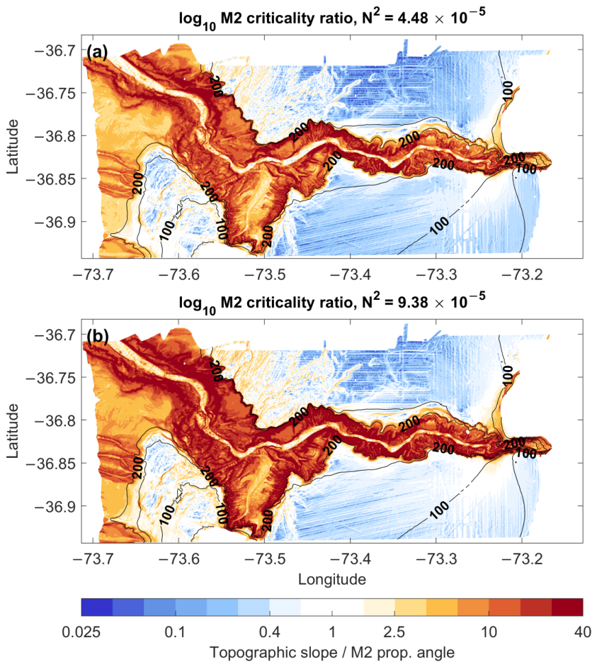
In general, the energy of the internal wave must be able to propagate shoreward and dissipate through turbulent processes to have enhanced mixing. As discussed previously, this condition depends on the relationship between the characteristic slope of the internal wave and the bottom slope. Specifically, energy can propagate and dissipate when the slope of the seabed is less than or equal to the slope of the wave, corresponding to subcritical or critical conditions. In the case of the BbC, the slope along the axis is relatively gentle (∼0.01), making it possible that, under appropriate stratification conditions, the energy of the semidiurnal internal tides can propagate onshore and induce mixing. During both study periods, the internal wave’s characteristic slope was greater than that of the canyon bottom, suggesting that the internal tidal energy propagated toward the coast (Figure 15).
Breaking of internal waves and bottom friction can ultimately lead to mixing through turbulent dissipation. However, Hotchkiss and Wunsch [16] demonstrated that, at least in the case of Hudson Canyon, dissipation due to bottom friction is an order of magnitude too small to account for the observed flux of internal wave energy into the canyon. Given the amplification of internal wave energy typically associated with submarine canyons, elevated levels of mixing are expected, as has been observed in several canyons worldwide, including Monterey and Gaoping Canyon [42,51].
A common characteristic of internal tides in eastern boundaries is that their energy tends to increase with stratification [53,54] and that their fluctuations are primarily responsible for the variability of the semidiurnal baroclinic energy [55]. In this context, it is worth highlighting that during P2, the internal wave slope approached the critical condition due to enhanced stratification. This scenario represents a more favorable setting for the generation and subsequent breaking of internal waves, which could favor enhanced mixing within the canyon. One limitation of the present study is that, due to data availability, only the vertical temperature structure was measured throughout the study periods, while the salinity profiles were limited to a single day during mooring deployment, restricting a more complete assessment of the temporal variability of the buoyancy frequency. Thus, the precise stratification-related mechanisms involved in this study should be interpreted carefully. An additional limitation of the present study is that the 2013 and 2014 observational programs differed not only in stratification state, but also in sampling season, mooring configuration, and vertical resolution. Therefore, the comparison between periods should be interpreted primarily as a qualitative, process-oriented contrast between two hydrographic and dynamical states observed at the canyon head, rather than as a strict separation of seasonal, interannual, or deployment-related effects.
The enhanced thermal stratification likely contributed to the increased energy observed in the baroclinic currents during P2 (2014). One possible explanation for this intensified stratification is the occurrence of unfavorable winds to upwelling during the sporadic passage of storms, leading to surface-layer subsidence. This was followed by subsurface cooling events associated with BbC. It is important to note that these cooling events were consistent with the passage of coastal trapped waves [10], which is consistent with enhanced upwelling events over the head of a canyon during the low sea-level phase of coastal trapped waves [56]. Additionally, freshwater input from the Biobio River, whose discharge peaks in winter [40,57], further stratified the surface layers, enhancing the overall stratification observed in 2014. These findings underscore the importance of future studies that aim to quantify the role of mixing driven by internal tides in supporting primary production in this region, as well as investigating in greater detail the specific contribution of BbC to the generation and breaking of internal tides.

5. Conclusions

The head of the Biobio Submarine Canyon is a dynamically active site of semidiurnal internal-tide variability, with the strongest and most coherent baroclinic motions observed during the more stratified 2014 period. During that deployment, semidiurnal baroclinic currents reached amplitudes of up to 17 cm s−1, were intensified near the surface and bottom, rotated anticyclonically, and were strongly aligned with the canyon axis. Their vertical structure was dominated by a first baroclinic mode, which explained more than 70% of the variance in 2014. The comparison between the two deployments suggests that stronger stratification favored the development of semidiurnal internal-tide-related motions over the canyon head. However, the relative roles of stratification, coastal trapped waves, freshwater input from the Biobio River, and canyon geometry could not be quantitatively separated, so these mechanisms should be regarded as plausible contributors rather than independently resolved effects. Likewise, although the observations indicate a dynamically favorable setting for enhanced internal-tide activity and potentially elevated mixing, direct turbulence and dissipation measurements were not available. These conclusions should also be interpreted in light of two main limitations: the 2013 and 2014 deployments differed in both season and observational configuration, and salinity was only available from snapshot hydrographic sampling, so temporal changes in buoyancy frequency were inferred mainly from temperature structure. Despite these limitations, the dataset provides a rare observational view of high-frequency motions directly over the canyon head. Future work should extend these observations with longer mooring records, concurrent salinity and turbulence measurements, and additional observations along the canyon and adjacent shelf, ideally complemented by process-oriented numerical modeling.

Author Contributions

Conceptualization, P.M. and M.S.; methodology, P.M.; formal analysis, P.M., M.S. and G.S.S.; investigation, M.S., P.M. and G.S.S.; resources, M.S. and G.S.S.; data curation, P.M.; writing—original draft preparation, M.S., P.M. and G.S.S. All authors have read and agreed to the published version of the manuscript.

Funding

The FONDECYT grant 1130648 has supported this work. Also, Gonzalo Saldías and Marcus Sobarzo have been partially supported by ANID Fondecyt Regular 1220167 and COPAS Coastal ANID FB210021.

Data Availability Statement

Data files are archived in the Zenodo repository (https://zenodo.org/records/19422184, accessed on 20 April 2026).

Conflicts of Interest

The authors declare no conflicts of interest.

References

  1. Shepard, F.P.; Goldberg, E.D.; Inman, D.L. Submarine Geology; Harper & Row: New York, NY, USA, 1963. [Google Scholar]
  2. Allen, S.E.; Durrieu de Madron, X. A review of the role of submarine canyons in deep ocean exchange with the shelf. Ocean. Sci. 2009, 5, 607–620. [Google Scholar]
  3. Hickey, B.M. Coastal submarine canyons. In Proceedings of the ‘Aha Huliko’a Hawaiian Winter Workshop on Flow–Topography Interactions, Honolulu, Hi, USA, 17–20 January 1995. [Google Scholar]
  4. Freeland, H.J.; Denman, K.L. A topographically controlled upwelling center off southern Vancouver Island. J. Mar. Res. 1982, 40, 1069–1093. [Google Scholar]
  5. Kenney, R.D.; Winn, H.E. Cetacean biomass densities near submarine canyons compared to adjacent shelf/slope areas. Cont. Shelf Res. 1987, 7, 107–114. [Google Scholar] [CrossRef]
  6. Allen, S.E.; Vindeirinho, C.; Thomson, R.E.; Foreman, M.G.; Mackas, D.L. Physical and biological processes over a submarine canyon during an upwelling event. Can. J. Fish. Aquat. Sci. 2001, 58, 671–684. [Google Scholar] [CrossRef]
  7. Thornburg, T.M.; Kulm, L.D. Sedimentation in the Chile Trench: Petrofacies and provenance. J. Sediment. Res. 1987, 57, 55–74. [Google Scholar] [CrossRef]
  8. Pineda, V. El cañón Submarino del Bío-Bío: Aspectos dináMicos y Ambientales. Doctoral Dissertation, Centro Eula, Universidad de Concepción, Región del Biobío, Chile, 1999. [Google Scholar]
  9. Daneri, G.; Dellarossa, V.; Quiñones, R.; Jacob, B.; Montero, P.; Ulloa, O. Primary production and community respiration in the Humboldt Current System off Chile and associated oceanic areas. Mar. Ecol. Prog. Ser. 2000, 197, 41–49. [Google Scholar] [CrossRef]
  10. Sobarzo, M.; Saldías, G.S.; Tapia, F.J.; Bravo, L.; Moffat, C.; Largier, J.L. On subsurface cooling associated with the Biobio River Canyon (Chile). J. Geophys. Res. Ocean. 2016, 121, 4568–4584. [Google Scholar]
  11. Ramos-Musalem, K.; Allen, S.E. The impact of locally enhanced vertical diffusivity on the cross-shelf transport of tracers induced by a submarine canyon. J. Phys. Oceanogr. 2019, 49, 561–584. [Google Scholar] [CrossRef]
  12. Saldías, G.S.; Allen, S.E. The influence of a submarine canyon on the circulation and cross-shore exchanges around an upwelling front. J. Phys. Oceanogr. 2020, 50, 1677–1698. [Google Scholar] [CrossRef]
  13. Kunze, E.; Rosenfeld, L.K.; Carter, G.S.; Gregg, M.C. Internal waves in Monterey submarine canyon. J. Phys. Oceanogr. 2002, 32, 1890–1913. [Google Scholar] [CrossRef]
  14. Nash, J.D.; Kunze, E.; Toole, J.M.; Schmitt, R.W. Internal tide reflection and turbulent mixing on the continental slope. J. Phys. Oceanogr. 2004, 34, 1117–1134. [Google Scholar] [CrossRef]
  15. Garrett, C.; Kunze, E. Internal tide generation in the deep ocean. Annu. Rev. Fluid Mech. 2007, 39, 57–87. [Google Scholar] [CrossRef]
  16. Hotchkiss, F.S.; Wunsch, C. Internal waves in Hudson Canyon with possible geological implications. Deep Sea Res. Part A Oceanogr. Res. Pap. 1982, 29, 415–442. [Google Scholar] [CrossRef]
  17. Gardner, W.D. Periodic resuspension in Baltimore Canyon by focusing of internal waves. J. Geophys. Res. Ocean. 1989, 94, 18185–18194. [Google Scholar]
  18. Petruncio, E.T.; Rosenfeld, L.K.; Paduan, J.D. Observations of the internal tide in Monterey Canyon. J. Phys. Oceanogr. 1998, 28, 1873–1903. [Google Scholar] [CrossRef]
  19. Carter, G.S.; Gregg, M.C.; Lien, R.C. Internal waves, solitary-like waves, and mixing on the Monterey Bay shelf. Cont. Shelf Res. 2005, 25, 1499–1520. [Google Scholar] [CrossRef]
  20. Hall, R.A.; Carter, G.S. Internal tides in Monterey submarine canyon. J. Phys. Oceanogr. 2011, 41, 186–204. [Google Scholar] [CrossRef]
  21. Waterhouse, A.F.; MacKinnon, J.A.; Nash, J.D.; Alford, M.H.; Kunze, E.; Simmons, H.L.; Polzin, K.L.; St. Laurent, L.C.; Sun, O.M.; Pinkel, R.; et al. Global patterns of diapycnal mixing from measurements of the turbulent dissipation rate. J. Phys. Oceanogr. 2014, 44, 1854–1872. [Google Scholar] [CrossRef]
  22. Wunsch, C.; Webb, S. The climatology of deep ocean internal waves. J. Phys. Oceanogr. 1979, 9, 235–243. [Google Scholar] [CrossRef][Green Version]
  23. Thornburg, T.M.; Kulm, L.D.; Hussong, D.M. Submarine-fan development in the southern Chile Trench: A dynamic interplay of tectonics and sedimentation. Geol. Soc. Am. Bull. 1990, 102, 1658–1680. [Google Scholar]
  24. Bernhardt, A.; Melnick, D.; Jara-Muñoz, J.; Argandoña, B.; González, J.; Strecker, M.R. Controls on submarine canyon activity during sea-level highstands: The Biobio canyon system offshore Chile. Geosphere 2015, 11, 1226–1255. [Google Scholar] [CrossRef]
  25. Sobarzo, M.; Figueroa, M.; Djurfeldt, L. Upwelling of subsurface water into the rim of the Biobıo submarine canyon as a response to surface winds. Cont. Shelf Res. 2001, 21, 279–299. [Google Scholar]
  26. Sobarzo, M.; Djurfeldt, L. Coastal upwelling process on a continental shelf limited by submarine canyons, Concepción, central Chile. J. Geophys. Res. Ocean. 2004, 109. [Google Scholar] [CrossRef]
  27. Vergara, O.A.; Figueroa, P.A.; Salas, C.; Vásquez, S.I.; Muñoz, R.; Saldías, G.S. The influence of the Biobio Canyon on the circulation and coastal upwelling/downwelling off central Chile. Cont. Shelf Res. 2024, 282, 105335. [Google Scholar] [CrossRef]
  28. Vargas, C.A.; Narváez, D.A.; Piñones, A.; Venegas, R.M.; Navarrete, S.A. Internal tidal bore warm fronts and settlement of invertebrates in central Chile. Estuar. Coast. Shelf Sci. 2004, 61, 603–612. [Google Scholar]
  29. Ramos, M. Corrientes de Marea en el Pacífico Sudoriental Frente a la Costa Central de Chile. Undergraduate Thesis, Escuela de Ciencias del Mar, Universidad Católica de Valparaíso, Región de Valparaíso, Chile, 1999. [Google Scholar]
  30. Aguirre, C.; Pizarro, O.; Sobarzo, M. Observations of semidiurnal internal tidal currents off central Chile (36.6° S). Cont. Shelf Res. 2010, 30, 1562–1574. [Google Scholar]
  31. Bravo, L.; Ramos, M.; Sobarzo, M.; Pizarro, O.; Valle-Levinson, A. Barotropic and baroclinic semidiurnal tidal currents in two contrasting coastal upwelling zones of Chile. J. Geophys. Res. Ocean. 2013, 118, 1226–1238. [Google Scholar]
  32. Jara-Muñoz, J.; Melnick, D.; Zambrano, P.; Rietbrock, A.; González, J.; Argandoña, B.; Strecker, M.R. Quantifying offshore fore-arc deformation and splay-fault slip using drowned Pleistocene shorelines, Arauco Bay, Chile. J. Geophys. Res. Solid Earth 2017, 122, 4529–4558. [Google Scholar]
  33. González-Acuña, J.; Arroyo-Suarez, E. Comparative methodologies for sounding reduction applied to a bathymetric survey referred to the WGS-84 ellipsoid, Executed in Concepcion Bay 550 and Gulf of Arauco, VIII Region, Chile. In Proceedings of the U.S. HYDRO 2013, New Orleans, LA, USA, 25–28 March 2013. [Google Scholar]
  34. Emery, W.J.; Thomson, R.E. Data Analysis Methods in Physical Oceanography; Elsevier: Amsterdam, The Netherlands, 2001. [Google Scholar]
  35. Pawlowicz, R.; Beardsley, B.; Lentz, S. Classical tidal harmonic analysis including error estimates in MATLAB using T TIDE. Comput. Geosci. 2002, 28, 929–937. [Google Scholar] [CrossRef]
  36. Holloway, P.E.; Chatwin, P.G.; Craig, P. Internal tide observations from the Australian north west shelf in summer 1995. J. Phys. Oceanogr. 2001, 31, 1182–1199. [Google Scholar] [CrossRef]
  37. Gilman, D.L.; Fuglister, F.J.; Mitchell, J.M., Jr. On the power spectrum of “red noise”. J. Atmos. Sci. 1963, 20, 182–184. [Google Scholar] [CrossRef]
  38. Gill, A.E. Atmosphere-Ocean Dynamics (International Geophysics Series); Academic Press: San Diego, CA, USA, 1982. [Google Scholar]
  39. Swart, N.C.; Allen, S.E.; Greenan, B.J.W. Resonant amplification of subinertial tides in a submarine canyon. J. Geophys. Res. Ocean. 2011, 116. [Google Scholar] [CrossRef]
  40. Sobarzo, M.; Shearman, R.K.; Lentz, S. Near-inertial motions over the continental shelf off Concepción, central Chile. Prog. Oceanogr. 2007, 75, 348–362. [Google Scholar] [CrossRef]
  41. Lafuente, J.G.; Sarhan, T.; Vargas, M.; Vargas, J.M.; Plaza, F. Tidal motions and tidally induced fluxes through La Linea submarine canyon, western Alboran Sea. J. Geophys. Res. Ocean. 1999, 104, 3109–3119. [Google Scholar] [CrossRef]
  42. Lee, I.H.; Lien, R.C.; Liu, J.T.; Chuang, W.S. Turbulent mixing and internal tides in Gaoping (Kaoping) submarine canyon, Taiwan. J. Mar. Syst. 2009, 76, 383–396. [Google Scholar] [CrossRef]
  43. Munk, W.; Wunsch, C. Abyssal recipes II: Energetics of tidal and wind mixing. Deep Sea Res. Part I Oceanogr. Res. Pap. 1998, 45, 1977–2010. [Google Scholar]
  44. Demers, S.; Legendre, L.; Therriault, J.C. Phytoplankton Responses to Vertical Tidal Mixing; Springer: New York, NY, USA, 1986; pp. 1–40. [Google Scholar]
  45. Margalef, R. Life-forms of phytoplankton as survival alternatives in an unstable environment. Oceanol. Acta 1978, 1, 493–509. [Google Scholar]
  46. Escribano, R.; Schneider, W. The structure and functioning of the coastal upwelling system off central/southern Chile. Prog. Oceanogr. 2007, 3, 343–347. [Google Scholar] [CrossRef]
  47. Thiel, M.; Macaya, E.C.; Acuna, E.; Arntz, W.E.; Bastias, H.; Brokordt, K.; Camus, P.A.; Castilla, J.C.; Castro, L.R.; Cortés, M.; et al. The Humboldt Current System of northern and central Chile: Oceanographic processes, ecological interactions and socioeconomic feedback. Oceanogr. Mar. Biol. Annu. Rev. 2007, 45, 195–344. [Google Scholar]
  48. Egbert, G.D.; Ray, R.D. Significant dissipation of tidal energy in the deep ocean inferred from satellite altimeter data. Nature 2000, 405, 775. [Google Scholar] [CrossRef]
  49. Munk, W. Once again: Once again—Tidal friction. Prog. Oceanogr. 1997, 40, 7–35. [Google Scholar] [CrossRef]
  50. Kantha, L.H.; Tierney, C.C. Global baroclinic tides. Prog. Oceanogr. 1997, 40, 163–178. [Google Scholar] [CrossRef]
  51. Carter, G.S.; Gregg, M.C. Intense, variable mixing near the head of Monterey Submarine Canyon. J. Phys. Oceanogr. 2002, 32, 3145–3165. [Google Scholar] [CrossRef]
  52. Jachec, S.M.; Fringer, O.B.; Gerritsen, M.G.; Street, R.L. Numerical simulation of internal tides and the resulting energetics within Monterey Bay and the surrounding area. Geophys. Res. Lett. 2006, 33. [Google Scholar] [CrossRef]
  53. Rosenfeld, L.K. Baroclinic semidiurnal tidal currents over the continental shelf off northern California. J. Geophys. Res. Ocean. 1990, 95, 22153–22172. [Google Scholar] [CrossRef]
  54. Lerczak, J.A.; Winant, C.; Hendershott, M. Observations of the semidiurnal internal tide on the southern California slope and shelf. J. Geophys. Res. Ocean. 2003, 108, 3068. [Google Scholar] [CrossRef]
  55. Baines, P.G. On internal tide generation models. Deep Sea Res. Part A Oceanogr. Res. Pap. 1982, 29, 307–338. [Google Scholar] [CrossRef]
  56. Saldías, G.S.; Ramos-Musalem, K.; Allen, S.E. Circulation and upwelling induced by coastal trapped waves over a submarine canyon in an idealized eastern boundary margin. Geophys. Res. Lett. 2021, 48, e2021GL093548. [Google Scholar] [CrossRef]
  57. Saldías, G.S.; Sobarzo, M.; Largier, J.; Moffat, C.; Letelier, R. Seasonal variability of turbid river plumes off central Chile based on high-resolution MODIS imagery. Remote Sens. Environ. 2012, 123, 220–233. [Google Scholar] [CrossRef]
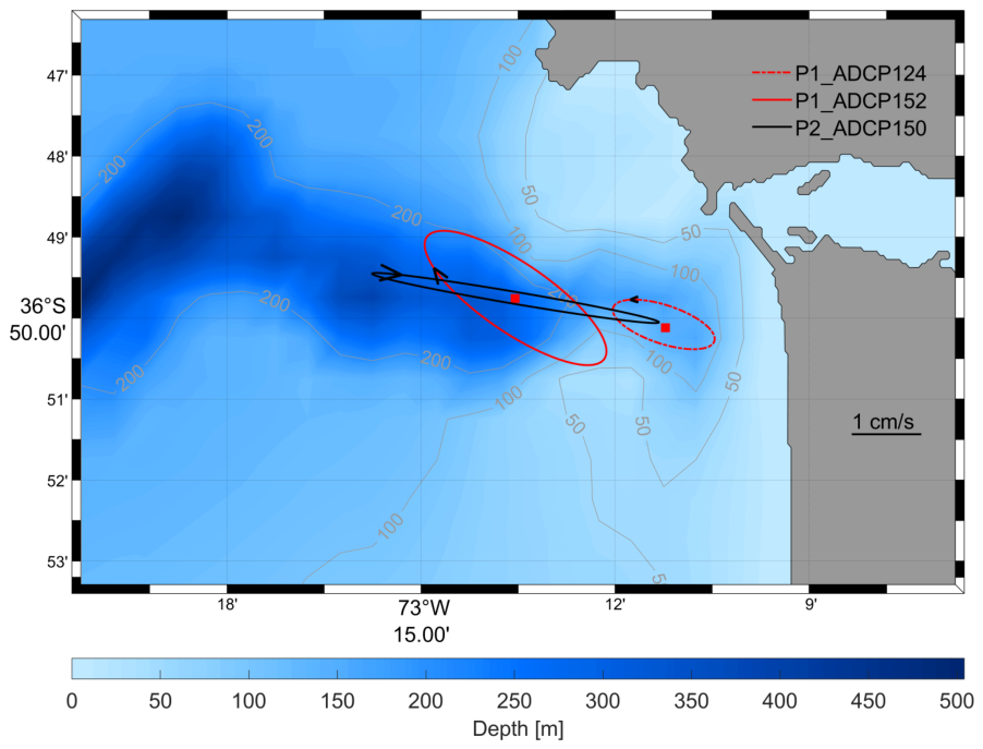
Figure 1. Study area with the location of oceanographic instruments. During P1 (2013), two ADCPs were located at 124 and 152 m depth, and one thermistor chain was recovered at 124 m. During P2 (2014), one ADCP and one thermistor chain were located at 150 m depth.
Jmse 14 00811 g001
Figure 2. (a) N-S and E-W wind components measured in Hualpen Point. (b) Sea level recorded in P1_ADCP124. (c) Water column hourly temperature close to the P1_ADCP124. (d) Band-pass temperature filter (between 9 and 15 h). The red dashed line represents the date of the selected profile for buoyancy frequency. The black dots in the vertical axis indicate the approximate depth of the thermistors. The deepest level (150 m) was covered by thermistor from P1_ADCP152. Cruise 1: November–December 2013.
Jmse 14 00811 g002
Figure 3. (a) N-S and E-W components of the wind (Hualpen Point). (b) Sea level recorded in P2_ADCP150. (c) Hourly temperature of the water column close to the P2_ADCP150. (d) Band-pass temperature filter (between 9 and 15 h). The black dashed line represents the date of the selected profile for buoyancy frequency. The black dots in the vertical axis indicate the approximate depth of the thermistors. The deepest level (150 m) was covered by thermistor from P2_ADCP150. Cruise 2: August–October 2014.
Jmse 14 00811 g003
Figure 4. Sea level autospectrum during Cruises 1 (spring 2013, red line) and 2 (winter–spring 2014, black line). The dashed lines indicate the frequency (cph) of the main tidal constituents used to calculate the F parameter.
Jmse 14 00811 g004
Figure 5. (a) Average temperature profile (°C) recorded during P1 and P2 cruises based on continuous temperature records at each depth level. Shades of color around the average indicate one standard deviation. (b) Selected buoyancy frequency profiles (cycles s−1) for each cruise (11 November 2013, and 11 September 2014). (c,d) Mean vertical current profile during Cruise 1 (2013) and Cruise 2 (2014).
Jmse 14 00811 g005
Figure 6. (ac) Total current along the MPA during Cruises 1 and 2. (df) Percentage of explained variance by the MPAs (in black) and MPA directions (in red) during Cruises 1 and 2. Here, 0° indicates eastward and negative directions rotate clockwise.
Jmse 14 00811 g006
Figure 7. Vertical structure of the rotating spectra of the total currents recorded by (a,b) P1_ADCP 124 m, (c,d) P1_ADCP 152 m, and (e,f) P2_ADCP 150 m. The yellow dashed lines represent the diurnal (D), inertial (I), and semidiurnal (SD) frequencies. The solid black contour delimits spectral peaks significant at the 95% level above a depth-dependent red-noise AR(1) background. The effective degrees of freedom and the corresponding 95% confidence interval in log 10 units are indicated in panel (b). Left panels: Anticlockwise. Right panels: Clockwise.
Jmse 14 00811 g007
Figure 8. Vertical structure of the rotating spectra of the baroclinic currents recorded by (a,b) P1_ADCP 124 m, (c,d) P1_ADCP 152 m, and (e,f) P2_ADCP 150 m. The yellow dashed lines represent the diurnal (D), inertial (I), and semidiurnal (SD) frequencies. The solid black contour delimits spectral peaks significant at the 95% level above a depth-dependent red-noise AR(1) background. The effective degrees of freedom and the corresponding 95% confidence interval in log 10 units are indicated in panel (b). Left panels: Anticlockwise. Right panels: Clockwise.
Jmse 14 00811 g008
Figure 9. (a,b) Vertical profiles of the rotation coefficient associated with semidiurnal (SD) and diurnal (D) baroclinic currents. (c) Variance profiles of total and baroclinic currents. Cruises 1 (2013) and 2 (2014).
Jmse 14 00811 g009
Figure 10. Ellipses of the barotropic semidiurnal current (M2) during the 2013 and 2014 cruises.
Jmse 14 00811 g010
Figure 11. Ellipses of the baroclinic semidiurnal current (M2) during the 2013 and 2014 cruises.
Jmse 14 00811 g011
Figure 12. (a) Variance profiles of semidiurnal baroclinic currents. The vertical dashed lines indicate the variance of the barotropic semidiurnal currents. (b) Percentage of total current variance explained by semidiurnal baroclinic currents.
Jmse 14 00811 g012
Figure 13. Vertical structure of the first empirical orthogonal mode (EOF) of the baroclinic semidiurnal current (u and v) for (a) P1_ADCP124, (b) P1_ADCP152, and (c) P2_ADCP150. The solid line (–) indicates the zonal component and the segmented line (-) the meridional component.
Jmse 14 00811 g013
Figure 14. Vector diagram of semidiurnal energy flux on the Biobio Canyon during the 2014 cruise, corresponding to the first dynamic mode.
Jmse 14 00811 g014
Figure 15. Log10 of the M2 internal tide criticality ratio for the Biobio Canyon region, computed for the stratification conditions observed during (a) November–December 2013 ( N 2 = 4.48 × 10 5 s−2) and (b) August–October 2014 ( N 2 = 9.38 × 10 5 s−2). Warm (cool) colors indicate supercritical (subcritical) topography. Black contours show the 100 and 200 m isobaths.
Jmse 14 00811 g015
Table 1. Instruments used and measurement periods. The variables recorded were the zonal and meridional currents (u,v), temperature (T) and sea level (SL).
CruiseInstrumentsLatitudeLongitudeDatesVariablesMeasurement Levels (m)
2013P1_ADCP152 m36°49.8′73°13.6′10 Nov to 10 Decu,v, T, SL12-144 (6)
P1_ADCP124 m36°50.1′73°11.2′10 Nov to 17 Decu,v, T, SL12 to 114 (each 2 m)
Thermistors36°50.1′73°11.2′10 Nov to 17 DecT10-20-30-40-60-100
2014P2_ADCP150 m36°49.8′73°13.6′16 Aug to 9 Octu,v, T, SL14 to 134 (each 6 m)
Thermistors36°49.8′73°13.6′16 Aug to 9 OctT10-15-20-30-40-60-100
Disclaimer/Publisher’s Note: The statements, opinions and data contained in all publications are solely those of the individual author(s) and contributor(s) and not of MDPI and/or the editor(s). MDPI and/or the editor(s) disclaim responsibility for any injury to people or property resulting from any ideas, methods, instructions or products referred to in the content.