Maneuverability Prediction of a Twin-Azimuth-Thruster Ship Using a CFD and MMG Coupled Model with Emphasis on Hydrodynamic Coupling Effects

Abstract

Predicting the maneuverability of ships equipped with twin azimuth thrusters remains challenging due to their complex hydrodynamic interactions. This study develops an integrated framework that combines Computational Fluid Dynamics (CFD) with an enhanced Manoeuvring Mathematical Group (MMG) Model. Using the platform supply vessel Hai Yang Shi You 661 as a case study, all requisite hydrodynamic derivatives and propeller coefficients were efficiently obtained through CFD-based captive model tests, including oblique towing and Planar Motion Mechanism tests, conducted in STAR-CCM+ 2206. A core contribution of this work is the systematic evaluation of how hydrodynamic model fidelity affects prediction accuracy. Numerical turning circle simulations were executed with three models of increasing complexity: one with only linear derivatives, a second incorporating nonlinear higher-order terms, and a third, full model that additionally includes nonlinear velocity coupling terms. The results, rigorously validated against full-scale trial data, demonstrate that while the basic CFD-MMG approach is feasible, the inclusion of nonlinear coupling terms is critical for achieving accurate predictions in large-amplitude maneuvers. This enhancement reduced the maximum error in tactical diameter prediction from over 25% to approximately 11.8%. Consequently, this study provides a validated and cost-effective framework for maneuvering the prediction of azimuth-thruster vessels and offers clear, quantitative guidance on the necessary level of model complexity for practical engineering applications.

1. Introduction

Ship maneuverability is a critical aspect of naval architecture and maritime operations, encompassing the study of how vessels respond to various control inputs and environmental conditions. With the increasing demands for enhanced ship maneuverability, the azimuth ships are becoming more widely used. The study of maneuverability in twin-azimuth-thruster vessels provides high-precision technical support for ship design and maneuvering control, thereby enabling the optimization of navigation strategies, the reduction in unnecessary energy consumption, and the improvement of safety and reliability in offshore operations, ultimately contributing to the Sustainable Development Goals (SDGs). By enhancing operational efficiency, it helps reduce fuel consumption and greenhouse gas emissions, thereby supporting SDG 7 (Affordable and Clean Energy) and SDG 13 (Climate Action) to a certain extent. Meanwhile, improving maneuvering performance and operational safety under complex sea conditions is also aligned with SDG 9 (Industry, Innovation and Infrastructure). However, the maneuverability of azimuth ships differs significantly from that of traditional rudder-propeller ships. This gap in knowledge can lead to empirical errors by deck officers. The significant interaction between the twin propellers, coupled with the complex hydrodynamic effects, further complicates the maneuverability of these vessels, making it a challenging technical bottleneck. Azimuth thrusters (pods) are typically located on both sides of the hull. During operation, their suction effect significantly alters the flow field around the stern, leading to nonlinear variations in the hydrodynamic forces acting on the hull, particularly in lateral force and yaw moment. Such interference becomes especially pronounced when the thrusters are at large deflection angles, or the vessel is under large drift angles. The pod (or duct) of an azimuth thruster generates substantial lateral force in oblique flow, which contributes significantly to the ship’s turning moment [1]. Azimuth-driven vessels generally exhibit excellent turning performance, but their course-keeping ability (straight-line stability) is comparatively weaker, requiring a balance between the two in design prediction. Since the thrusters can rotate 360°, the vessel often operates in a state of highly nonlinear motions characterized by large drift angles and large thruster angles. The hydrodynamic derivatives of the hull exhibit strong nonlinearity, and coupling effects among surge, sway, and yaw motions are significant. Mathematical models that only include linear terms tend to produce large errors in high-amplitude maneuvers [2]. The research in this area has attracted significant attention over the years, driven by the need for more accurate predictions of ship behavior in different scenarios.

The primary methods for researching ship maneuverability include scale model tests in towing tanks, full-scale ship trials, numerical simulations using Computational Fluid Dynamics (CFD), and parameter identification through application tests or real ship data. Currently, approaches that combine theoretical calculations with experimental adjustments are also widely employed. The two most commonly employed methods for predicting ship maneuverability are the Abkowitz method and the modular method developed by the Japanese Mathematical Modeling Group (MMG), primarily applied to conventional propeller-rudder ships [3]. However, ships equipped with azimuth thrusters, which can generate thrust in any direction and often have non-traditional hull shapes, cannot be directly applied to the MMG methodology. Early research in ship maneuverability relied heavily on empirical formulas and physical model tests. Among these, the MMG model emerged as a widely accepted semi-empirical method for predicting ship maneuverability. Hirano et al. [4] discussed methods for calculating ship maneuvering motion with MMG model. The MMG model decomposes the forces and moments acting on the ship into components from the hull, propeller, and rudder, offering a relatively straightforward approach to analyzing ship behavior. However, the MMG model has limitations, especially when dealing with complex environments such as shallow waters, confined channels, or interactions between multiple vessels. Despite this, the development of appropriate interaction coefficients for hull-pod propeller systems within the MMG framework makes it a viable approach for predicting the maneuverability of pod-driven ships as well [5]. The introduction of Computational Fluid Dynamics (CFD) has brought significant advancements to ship maneuverability research. CFD allows for detailed simulation of fluid dynamics around the ship, offering insights into hydrodynamic forces and moments that are challenging to capture with traditional methods. Previous studies [6] have highlighted that CFD can enhance the accuracy of maneuvering predictions by resolving complex fluid interactions that influence ship behavior. Wang et al. [7] emphasized the ability of CFD to model non-linear hydrodynamic effects, providing a more comprehensive understanding of ship maneuverability. Yasukawa, H. introduced the standard MMG methodology and provided a detailed discussion on its application in ship maneuvering predictions [8]. Yoshimura [9] combined Computational Fluid Dynamics (CFD) with the model to simulate ship maneuvering in shallow water. The results help to understand how shallow water conditions affect ship handling. Delefortrie et al. [10] established a maneuvering motion model for an inland river container ship with two full-revolving propellers by towing experiments. To bridge the gap between empirical and computational approaches, researchers have explored integrating CFD with MMG models. This hybrid approach combines the efficiency of MMG with the detailed hydrodynamic data provided by CFD. Lu Z et al. [11] demonstrated how CFD-based MMG models can improve maneuvering simulations by incorporating more accurate fluid dynamics information. This integration is particularly useful for simulating complex maneuvering scenarios where environmental factors play a significant role. Xie [12] reviewed the application of CFD for simulating ship maneuverability, analyzing the strengths and limitations of existing models and also examined at the integration of CFD with traditional maneuvering prediction methods. Loan T M. [13] explored the application to surface ship maneuverability, providing foundational insights and methodologies that have informed subsequent research in the field. Delefortrie implemented a new mathematical model in the ship maneuvering simulator and compared it against free running model tests, which, after slight tuning, seemed capable of capturing the maneuvering motion of the ship in six DOFs [14]. Delefortrie [15] also predicted the maneuvering characteristics of a container ship, discussing the accuracy and computational efficiency of the approach compared to traditional methods. To bridge the gap between empirical and computational approaches, researchers have explored integrating CFD with MMG models. This hybrid approach combines the efficiency of MMG with the detailed hydrodynamic data provided by CFD. Hasegawa et al. (2016) demonstrated how CFD-based MMG models can improve maneuvering simulations by incorporating more accurate fluid dynamics information [16]. This integration is particularly useful for simulating complex maneuvering scenarios where environmental factors play a significant role. Tang [17] used CFD to investigate the effects of shallow water on ship maneuverability, revealing how these conditions alter hydrodynamic forces. Lee [18] explored ship behavior in restricted waters, providing valuable insights for port design and operational planning. These studies demonstrate the versatility of CFD in addressing the challenges of varying environmental factors. The ongoing development of CFD technology and its integration into real-time simulation and automated control systems are paving the way for more accurate and practical maneuverability predictions. Ship maneuverability research has progressed from empirical methods to sophisticated computational techniques. The integration of CFD with traditional models like MMG has significantly improved the precision of maneuverability predictions. As technology continues to advance, the field is poised to achieve even greater accuracy and applicability, ultimately enhancing maritime safety and operational efficiency.

As for the study on the propellers, the RANS method, combined with turbulence models, has been extensively validated against experimental data and is known for its robustness in predicting the flow around the propeller blades [19]. The Sliding Mesh and Overset Mesh methods are often employed in simulations to capture the transient flow characteristics and interaction effects between the propeller and the surrounding flow field. However, these methods require significant computational resources and time, which can limit their application in large-scale or high-fidelity simulations [20]. The Multiple Reference Frame (MRF) method is another popular approach, particularly in propeller open water tests, due to its ability to model steady-state flow conditions efficiently. However, the MRF method tends to introduce errors in self-propulsion simulations because it does not account for wake asymmetry, leading to less accurate predictions of propeller performance [21]. Moreover, the Body Force (BF) method, which uses a virtual actuator disk, has been applied to simplify the propeller modeling process. While this approach is computationally efficient, it struggles to accurately capture self-propulsion factors, as it does not resolve the propeller geometry in detail [22]. Recent advancements in high-performance computing and hybrid modeling approaches, such as the integration of CFD with experimental data, have further enhanced the accuracy and applicability of propeller simulations. These developments are critical for optimizing propeller designs and improving the overall efficiency of marine propulsion systems, ultimately contributing to more sustainable maritime operations [23].

The foregoing analysis indicates that extensive research has been conducted by both domestic and international scholars on the maneuverability of azimuth-thruster vessels, CFD-based hydrodynamic simulations, and significant progress has been achieved. However, several key issues still require further in-depth and systematic investigation, particularly with regard to high-accuracy maneuvering prediction for twin-azimuth-thruster vessels:

(1) Incomplete model accuracy evaluation framework: Existing studies typically employ hydrodynamic models with a single level of complexity, lacking systematic comparisons and quantitative evaluations among models of different fidelity levels (e.g., linear, nonlinear, and fully coupled models). As a result, it is difficult to clearly identify the specific contributions of nonlinear and coupling terms to prediction accuracy, and to provide guidance for selecting an appropriate model complexity in engineering applications.

(2) Insufficient refined modeling for twin-azimuth-thruster vessels: Most current studies still follow the traditional modeling approach developed for propeller–rudder systems. The unique characteristics of twin azimuth thrusters, including mutual interaction between the two propellers and the strong coupling effects between the propellers and the hull, are not adequately captured. This limitation reduces the model fidelity under large-amplitude maneuvering conditions.

(3) Limited prediction accuracy under large-amplitude maneuvering conditions: Although existing methods generally provide acceptable predictions under conventional operating conditions, their accuracy significantly deteriorates in highly nonlinear conditions, such as large drift angles and large turning motions. The prediction error of key parameters, such as turning diameter, typically remains in the range of 15–25%, which is insufficient for high-precision engineering applications.

(4) Lack of mechanistic and quantitative understanding of coupling effects: Although the importance of sway–yaw coupling effects is widely recognized, there is still a lack of in-depth physical interpretation and quantitative evaluation regarding the extent to which these coupling terms dominate the maneuvering behavior and how much error is introduced when they are neglected.

To address the above issues, this study develops an integrated maneuverability prediction framework for twin-azimuth-thruster vessels by coupling CFD-based virtual captive tests with an enhanced MMG mathematical model. The platform supply vessel “Hai Yang Shi You 661” is selected as the case study. The remainder of this paper is organized as follows. Section 2 details the mathematical model, including the extended MMG equations and the decomposition of forces for twin azimuth thrusters. Section 3 describes the numerical simulation setup, including the computational domain, mesh, test conditions, and the process for identifying hydrodynamic derivatives. Section 4 presents the maneuvering simulation results, compares the performance of three hydrodynamic models of varying fidelity against full-scale trial data, and provides a discussion of the findings. Finally, Section 5 summarizes the main conclusions of this work.

The main contribution of this work lies in the proposed progressive hydrodynamic modeling algorithm, in which three maneuvering models with increasing fidelity are systematically established and compared, including the following: (1) a linear derivative model, (2) a nonlinear uncoupled model with higher-order terms, and (3) a fully coupled nonlinear model. Based on CFD-generated PMM, oblique towing and open-water test data, all hydrodynamic derivatives of the hull and parameters of thrusters are identified through the least-squares method and then implemented into the maneuvering simulation framework. This algorithm enables a quantitative evaluation of how model complexity influences prediction accuracy in large-amplitude maneuvers. Validation against full-scale sea trial data demonstrates that the proposed fully coupled model significantly improves turning-circle prediction accuracy, reducing the maximum error from over 25% to approximately 11.8%.

2. Mathematical Model

In this study, the MMG method for predicting maneuvering abilities has been extended to accommodate ships equipped with azimuth propellers. Captive model tests using the Planar Motion Mechanism (PMM) were conducted to enhance the equations of motion by incorporating hull hydrodynamic derivatives and hull-pod propeller interaction coefficients.

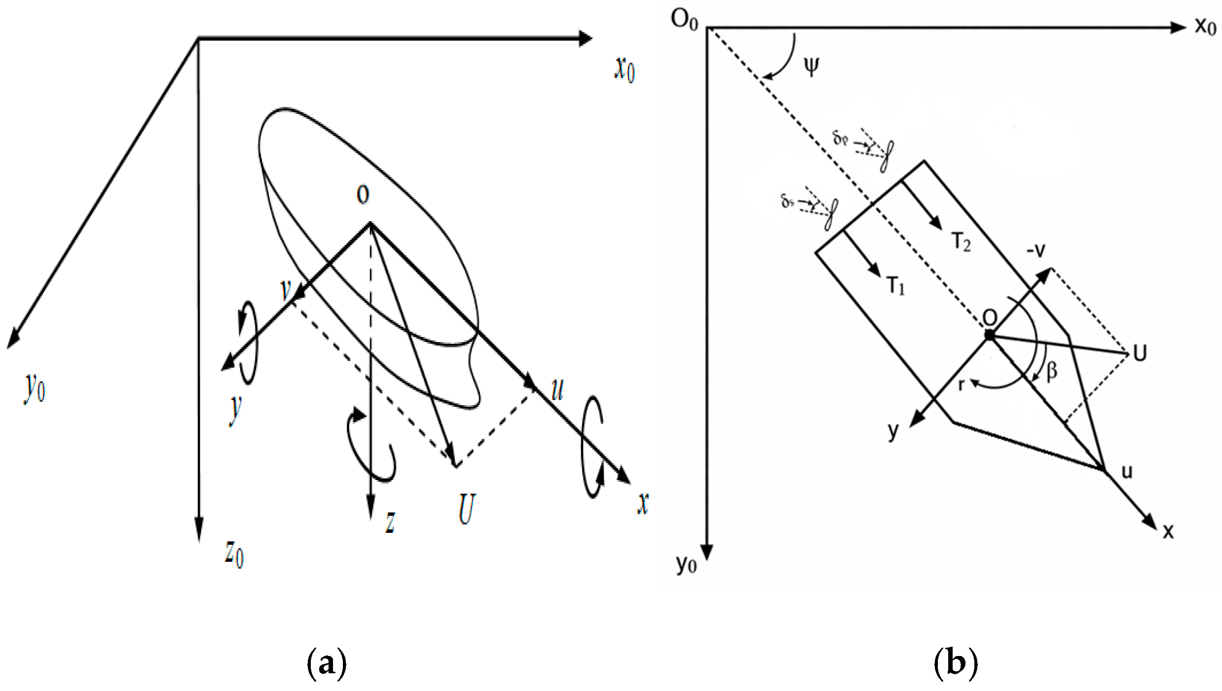
To describe the maneuvering motion of the twin-azimuth-thruster vessel in the horizontal plane, two coordinate systems are adopted in this study, namely, the inertial coordinate system and the body-fixed coordinate system, as shown in Figure 1. As shown in Figure 1a, the inertial coordinate system O₀–x₀y₀z₀ is used to describe the position of the vessel and serves as the reference frame. In this system, the x₀-axis points toward the geographic north, the y₀-axis points toward the east, and the z₀-axis points toward the center of the earth. The body-fixed coordinate system, also referred to as the ship-fixed coordinate system O–xyz, is used to describe the vessel motion and the forces acting on the vessel. The origin of this coordinate system is located at midship. The positive x-axis points toward the bow, the positive y-axis points toward the starboard side, and the positive z-axis points downward toward the keel.

The inertial coordinate system is mainly used to output the simulated trajectory, while the body-fixed coordinate system is employed to solve the hydrodynamic forces and velocity responses of the vessel. The relationship between the vessel position and motion parameters in the horizontal plane is illustrated in Figure 1b. The angle between the ship centerline and the x₀-axis is defined as the heading angle ψ. The velocity components of the vessel in the body-fixed coordinate system along the x- and y-axes are denoted by u and v, representing the surge velocity and sway velocity, respectively. The angular velocity of the vessel rotating about the z-axis is denoted by r.

Neglecting external disturbances such as wind, waves, and current, and focusing on planar maneuvering motion, the vessel motion can be simplified as a three-degree-of-freedom problem consisting of surge, sway, and yaw. The governing equations of planar maneuvering motion can then be written as Equation (1).

$$\left\{\begin{array}{l}X=m(\dot{u}-vr-x_G{r}^2)\hfill \\ Y=m(\dot{v}+ur+x_G\dot{r})\hfill \\ N=I_z\dot{r}+m{x}_G(\dot{v}+ur)\hfill \end{array}\right.$$

(1)

where m is the mass of the ship, u, v and r are the surge, sway, and yaw velocities. $\dot{u}$, $\dot{v}$ and $\dot{r}$ are the surge, sway, and yaw accelerations. $I_Z$ is the moment of inertia with respect to the z-axis, $X$ and $Y$ represent the forces acting in the longitudinal and lateral directions. $N$ is the moment with respect to the z-axis. $x_G$ represent the longitudinal position of the center of gravity relative to the reference point.

In the MMG model, the forces and moments acting on the study ship can be represented as Equation (2):

$$\left\{\begin{array}{l}X=X_H+X_P\hfill \\ Y=Y_H+Y_P\hfill \\ N=N_H+N_P\hfill \end{array}\right.$$

(2)

where the subscripts H and P refer to hull and pod propellers, respectively.

2.1. Hydrodynamic Forces and Moment Acting on the Hull

Hydrodynamic derivatives are key parameters in mathematical models used to describe the forces and moments acting on a ship as it moves through water. These derivatives capture the complexity of the forces involved, encompassing both linear and nonlinear effects. When the ship’s motion parameters are small, higher-order terms are often omitted. Consequently, the forces and moments acting on the hull can be simplified as Equation (3):

$$\left\{\begin{array}{l}{X}_H=R_0+X_u\Delta u\hfill \\ Y_H=Y_{v}v+Y_{r}r\hfill \\ N_H=N_{v}v+N_{r}r\hfill \end{array}\right.$$

(3)

where R₀ is ship resistance in straight moving condition, $X$, $Y$, $N$ with subscripts are the hydrodynamic derivatives.

2.2. Hydrodynamic Forces and Moment Due to Propellers

To simplify the situation, this study only considers the case of synchronous maneuvering with twin azimuth thrusters. The longitudinal and lateral forces can be expressed as Equation (4):

$$\left\{\begin{array}{l}{X}_p=(1-t_p)(T_p\cos \delta +T_s\cos \delta )\hfill \\ Y_p=-(1-t_p)(T_p\sin \delta +T_s\sin \delta )\hfill \\ N_p=(1-t_p)(T_p\cos \delta -T_s\cos \delta )y_p-Y_p{x}_p\hfill \end{array}\right.$$

(4)

where $T_P$ and $T_S$ represent the port side and starboard side of the thrusters, $t_p$ is the thrust coefficient, $x_p$ and $y_p$ are the coordinates of the thruster. In the present work, the forces $T_P$ and $T_S$ can be described as Equation (5):

$$\left\{\begin{array}{l}{T}_p=\rho n^2{D}^4{K}_{Tp}\hfill \\ T_s=\rho n^2{D}^4{K}_{Ts}\hfill \end{array}\right.$$

(5)

The thrust coefficient $K_T$ as a function of the advance ratio J can be expressed using empirical or theoretical relationships derived from experimental data or computational models. The advance ratio J is defined as Equation (6):

$$J=(1-{\omega }_T){\displaystyle \frac{V}{nD}}$$

(6)

where ${\omega }_T$ is the effective wake fraction at the propeller position in straight moving. Alternatively, the thrust coefficient can also be represented in Equation (7) using polynomial or other empirical fits based on experimental data:

$$\left\{\begin{array}{l}{K}_{TP}=K_{T{P}_0}+K_{T{P}_1}J+K_{T{P}_2}{J}^2\hfill \\ K_{TS}=K_{T{S}_0}+K_{T{S}_1}J+K_{T{S}_2}{J}^2\hfill \end{array}\right.$$

(7)

2.3. Study Ship

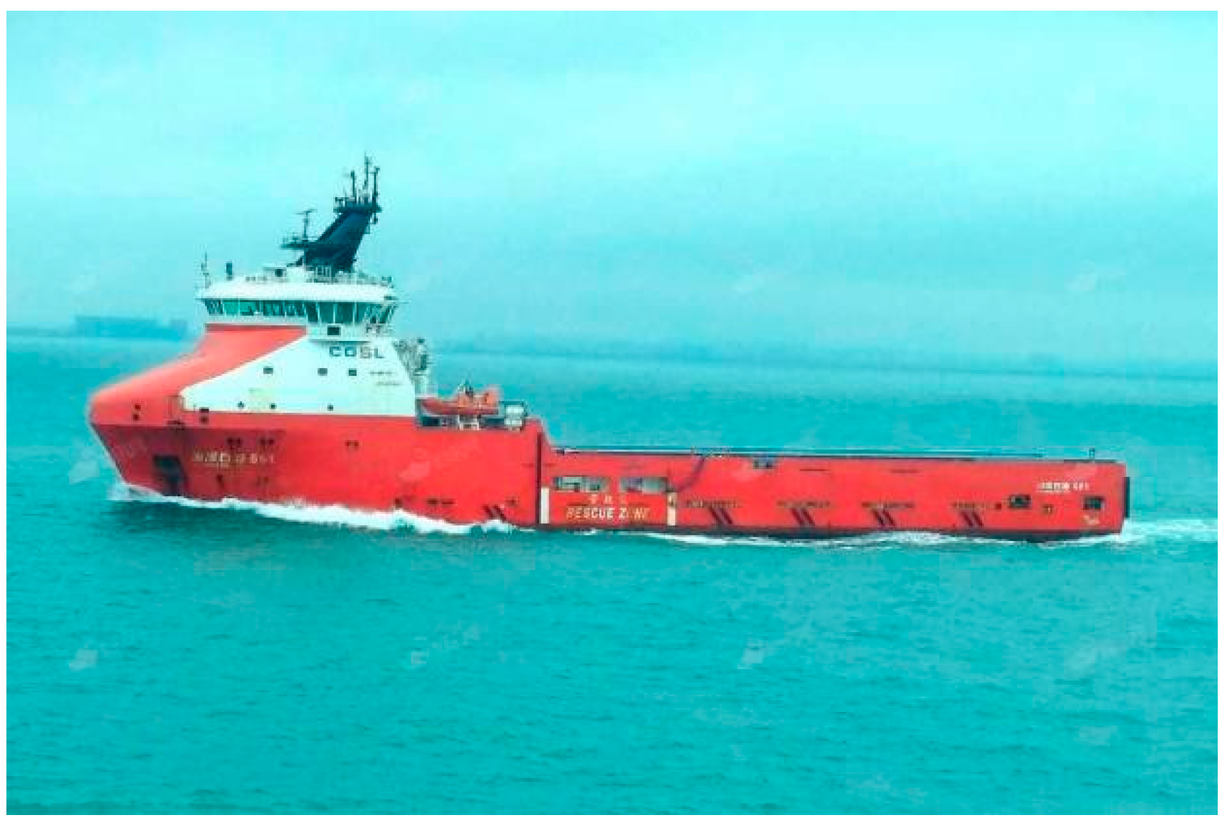
The study ship “Hai Yang Shi You 661”, owned and operated by China Oilfield Services Limited (COSL), is a highly specialized offshore engineering vessel equipped with advanced azimuth thrusters at port and starboard sides symmetrically. These thrusters provide the ship with exceptional maneuverability and precise positioning capabilities, making it ideal for complex offshore operations such as subsea installation, pipeline laying, and maintenance of offshore platforms.

To analyze the hydrodynamic performance of the hull and thrusters, the ship model is simplified by removing both the superstructure and the pods. The geometry of the ship and its principal parameters are displayed in Figure 2 and

Table 1. Principal parameters of the ship “Hai Yang Shi You 661”.

Principal Particular	Value	Unit
Length overall, Loa	85.400	m
Length between perpendiculars, Lpp	77.700	m
Molded breadth, B	20.000	m
Molded depth, D	8.600	m
Designed draft, d	7.163	m
Displacement	3649.35	t
Longitudinal position of gravity center, xG	4.294	m
Block coefficient, Cb	0.763
Longitudinal position of thrusters, xp	−37.390	m
Lateral position of thrusters, yp	±4.303	m

.

3. Numerical Simulation

Based on the STAR-CCM+ 2206 platform, this study conducted a series of captive model tests to simulate the ship’s hydrodynamic behavior. The hydrodynamic derivatives related to sway (v) were obtained from oblique towing tests, while those related to yaw (r) and the coupled terms were obtained from pure yaw (PMM) tests. The principal parameters of the vessel “Hai Yang Shi You 661” are listed in Table 1.

3.1. Physical Modes

To address the conditions involving turbulence, multiphase flow, and complex boundary layer behavior, this study employed the Reynolds-Averaged Navier–Stokes (RANs) equations, coupled with the widely used SST $k-\omega$ turbulence model and the Volume of Fluid (VOF) algorithm. The RANS equations (Reynolds-Averaged Navier–Stokes equations) are derived from the Navier–Stokes equations through time-averaging or statistical averaging, and they are used to describe the mean characteristics of turbulent flow. The core idea of the RANS equations is to decompose the physical quantities in the flow into mean and fluctuating components, thereby transforming the problem of turbulence into one of solving for the mean flow characteristics. The RANS equations are shown by Equation (8). The Reynolds stress tensor is a key term in the RANS equations, representing the additional momentum transfer induced by turbulence. This term is a nonlinear one obtained through averaging, which results in the RANS equations being an unclosed system of equations.

$${\displaystyle \frac{\partial {\overline{u}}_i}{\partial t}}+{\overline{u}}_j{\displaystyle \frac{\partial {\overline{u}}_i}{\partial x_j}}=-{\displaystyle \frac{1}{\rho }}{\displaystyle \frac{\partial \overline{p}}{\partial x_i}}+\nu {\displaystyle \frac{{\partial }^2{\overline{u}}_i}{\partial x_j^2}}-{\displaystyle \frac{\partial \overline{u_{i^{\prime }}{u}_{j^{\prime }}}}{\partial x_j}}$$

(8)

where ${\overline{\mathit{u}}}_{\mathit{i}}$ is the mean velocity component. $\overline{p}$ is the mean pressure. $\nu$ is the kinematic viscosity coefficient. $\rho$ is the fluid density. $\overline{u_i^{\prime }{u}_j^{\prime }}$ is the Reynolds stress tensor, representing the stress induced by turbulent fluctuations.

To close the RANS equations, turbulence models are introduced to relate the Reynolds stresses to the mean flow characteristics. Common turbulence models include the $k-\epsilon$ model, the $k-\omega$ model, and others. The $k-\omega$ turbulence model and the $k-\epsilon$ turbulence model are commonly used in Computational Fluid Dynamics (CFD). Each has different applications, strengths, and weaknesses. Compared to the $k-\epsilon$ model, the $k-\omega$ model has the following main advantages:

(1) The $k-\omega$ model provides higher accuracy in near-wall regions because the definition and solution method of (turbulence frequency) make it more suitable for handling low Reynolds number regions, such as the near-wall layer.

(2) The $k-\omega$ model performs better in handling separated flows and adverse pressure gradients (such as separation zones). This is because it can more accurately predict boundary layer behavior, whereas the $k-\epsilon$ model may underestimate turbulence intensity in these situations, leading to less accurate predictions.

(3) Since the $k-\omega$ model directly solves for turbulence quantities in the near-wall region, it does not rely on wall functions like the $k-\epsilon$ model. This makes the $k-\omega$ model superior in flows with complex geometries or strong separation phenomena.

(4) The $k-\omega$ model is more accurate than the $k-\epsilon$ model in low Reynolds number flows, as it can handle these flows without special adjustments. This makes it better suited for simulating flows in low Reynolds number environments, such as small-scale devices or low-speed flows. Its fundamental equations are as shown in Equation (9):

$$\left\{\begin{array}{l}{\displaystyle \frac{\partial k}{\partial t}}+U_j{\displaystyle \frac{\partial k}{\partial x_j}}=P_k-{\beta }^{\ast }k\omega \left[\left(\nu +{\sigma }_k{\nu }_t\right){\displaystyle \frac{\partial k}{\partial x_j}}\right]\\ {\displaystyle \frac{\partial \omega }{\partial t}}+U_j{\displaystyle \frac{\partial \omega }{\partial x_j}}={\displaystyle \frac{\gamma \omega }{k}}{P}_k-\beta {\omega }^2+{\displaystyle \frac{\partial }{\partial x_j}}\left[\left(\nu +{\sigma }_{\omega }{\nu }_t\right){\displaystyle \frac{\partial \omega }{\partial x_j}}\right]\end{array}\right.$$

(9)

where $k$ is the turbulence kinetic energy. $U_j$ is the mean velocity component. $P_k$ is the production term of turbulence kinetic energy. $\omega$ is the specific dissipation rate. $v$ is the kinematic viscosity. $v_t$ is the turbulent viscosity. ${\beta }^{\ast },{\sigma }_k,\gamma ,\beta$ and ${\sigma }_{\omega }$ are the empirical constants.

The turbulent viscosity is calculated by Equation (10):

$${\nu }_t={\displaystyle \frac{k}{\omega }}$$

(10)

The SST (Shear Stress Transport) $k-\omega$ model is an improved version of the $k-\omega$ model, incorporating advantages from the $k-\epsilon$ model. It uses the $k-\omega$ model in regions near the wall, while gradually transitioning to the $k-\epsilon$ model in the free-stream regions away from the wall, in order to avoid the excessive turbulent viscosity that can occur with the $k-\omega$ model in free-stream areas. VOF (Volume of Fluid) is an algorithm used to handle multiphase flows, such as gas–liquid two-phase flows. The core idea of the VOF algorithm is to determine the interface position between different phases by tracking the volume fraction of the fluids. The VOF algorithm used in STAR-CCM+ 2206 can accurately capture fluid interfaces, making it particularly suitable for simulating free surface flows, wave problems, and gas–liquid mixed flows.

3.2. Computational Domain and Grid

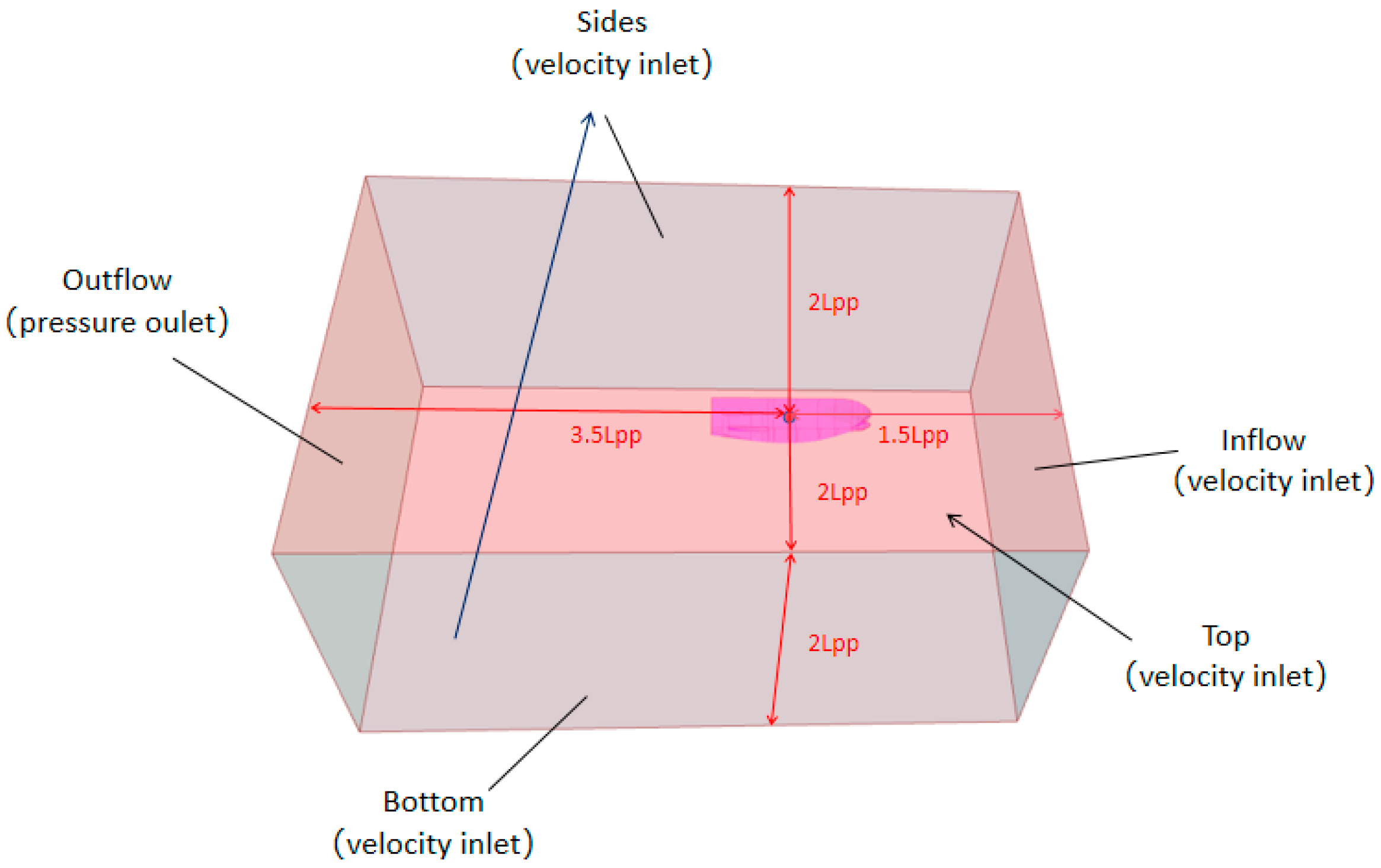
The calculations of the series of PMM tests were carried out in a rectangular domain displayed in Figure 3. The inflow boundary is 1.5 L_pp ahead of the center of the ship, 3.5 L_pp from the center to the outlet boundary for wake development, 2 L_pp from the center to sides and 2 L_pp in the depth for the whole domain as a deep-water situation. The hull is defined as a rigid body for no-slip wall.

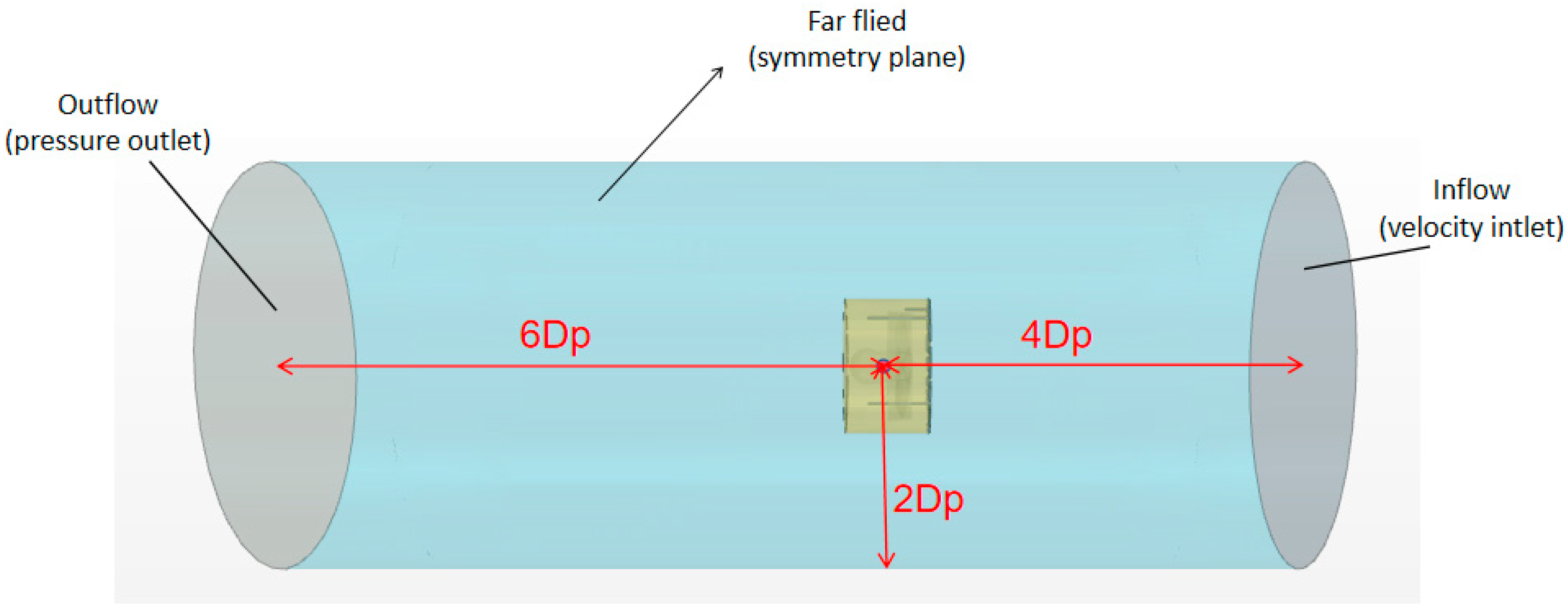
The propeller open water performance was conducted in a cylinder domain, as shown as Figure 4. The blue peripheral cylinder was set as the static region and the yellow inner cylinder was set as the rotating region. The sliding mesh method was used to handle flow problems in rotating regions. It addresses the relative motion between different regions by dividing the flow domain into stationary and rotating parts. The sliding mesh method does not require remeshing or deformation of the grid; instead, it manages the relative motion through a sliding interface between the rotating and stationary regions. The information exchange occurs at the interface of the static and rotating regions. 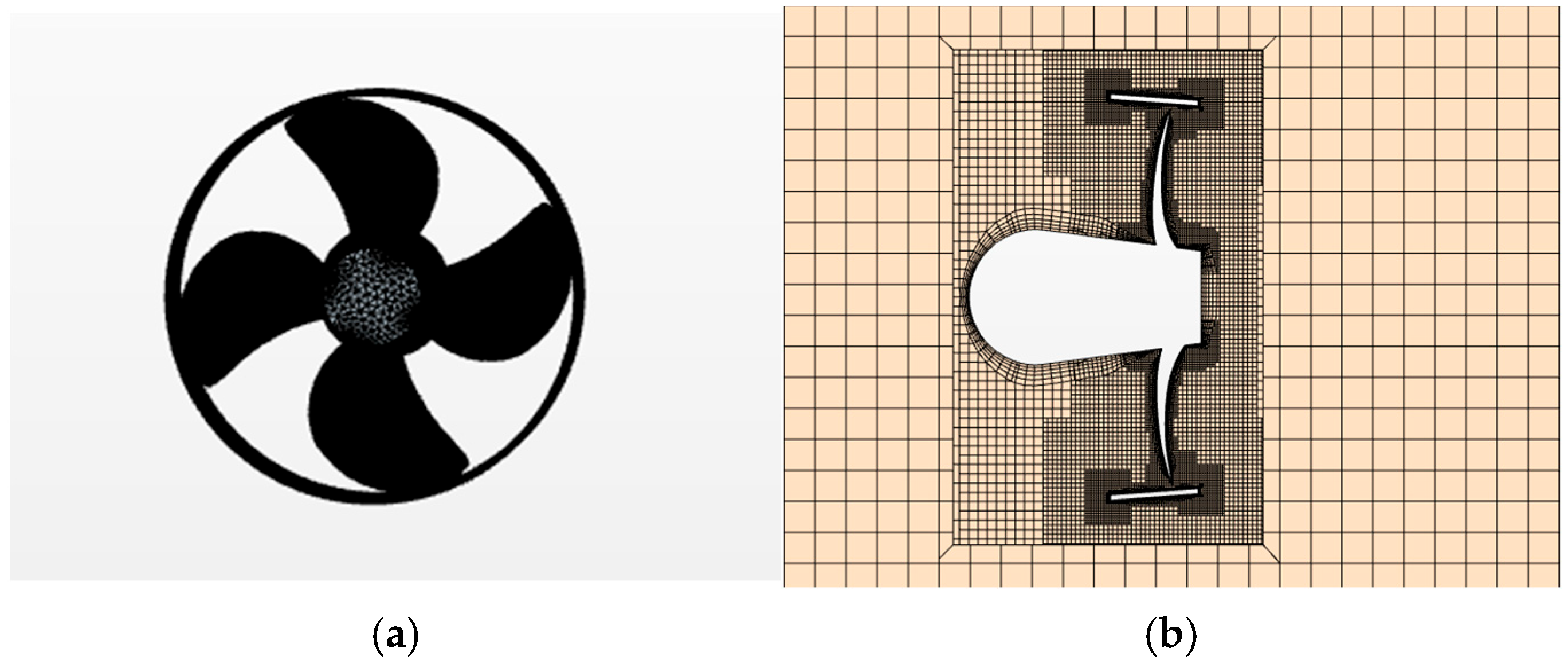Figure 5 shows the mesh of the propeller and the calculation domain.

In a grid independence test, $R_G$ typically refers to the Grid Convergence Rate. It is used to quantify how the simulation results change as the grid is refined. $R_G$ is usually calculated based on the physical quantities obtained from simulations with different levels of grid refinement. In this work, three sets of mesh densities were selected in the self-propulsion tests. The results are displayed in

Table 2. Results of the grid independence test.

Grid Number (Million)	Calculated Value (kN)	Experiment Value (kN)	Error
1.21	341.4	374.3	8.79%
3.48	359.5	374.3	3.95%
6.78	365.1	374.3	2.46%

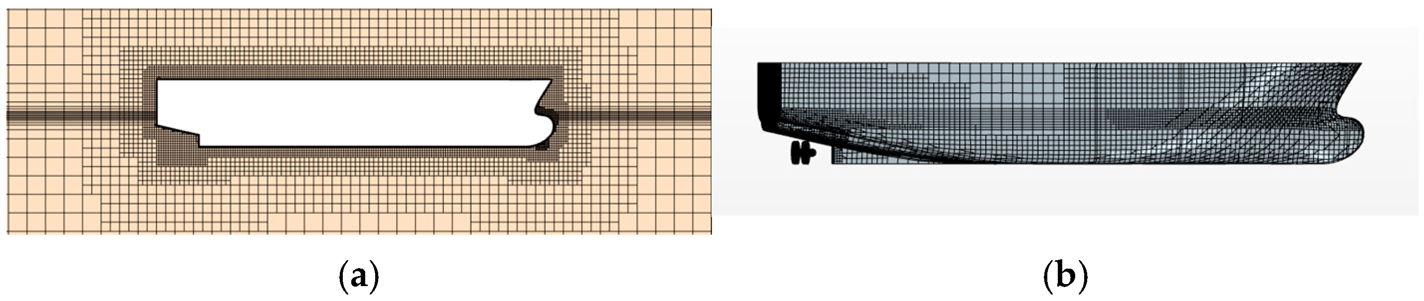
. Considering factors such as the accuracy of the calculations and the computational costs, 3.48 was the final choice. In this case, the convergence rate $R_G$ was calculated to be 0.36, which satisfied the conditions. The result of the grid is shown in Figure 6.

3.3. Test Conditions

A series of simulations were conducted, as detailed in

Table 3. Conditions for all numerical tests.

Tests	β (°)	$\mathit{J}$	A (M)	Ψ0 (°)	f (HZ)
Self-propulsion	$0$	—	—	—	—
Oblique tests	$0,\pm 4,\pm 8,\pm 12,\pm 20$	—	—	—	—
Pure yaw tests	—	—	$1\%Lpp,0.05\%Lpp$	$10,20$	$0.02,0.04,0.1$
Open water performance	—	$0.1–0.8$	—	—	—

. The ship speed u was maintained at the design speed of 6.17 m/s (corresponding to the Froude number of approximately 0.224) for all hull force tests. The Froude number (Fr) is an important dimensionless parameter used to characterize the relative effects of inertial and gravitational forces during ship motion. It is defined as Equation (11):

$$F_r={\displaystyle \frac{U}{\sqrt{gL}}}$$

(11)

where U is the ship speed, g is the gravitational acceleration, and L is the characteristic length, typically taken as the ship length. The Froude number reflects the intensity of wave-making effects and is one of the key parameters in analyzing ship resistance characteristics and maneuvering performance. Based on hydrodynamic characteristics, the Froude number can generally be classified into several regimes. When F_r < 0.2, the vessel operates in the low-speed regime, where viscous effects dominate and wave-making resistance is relatively small. For 0.2 < F_r < 0.4, the vessel is in the moderate-speed regime, where wave-making effects become increasingly significant, and the total resistance is governed by both viscous and wave-making components. When F_r > 0.4, the vessel enters the high-speed regime, in which wave-making resistance becomes dominant and strong nonlinear free-surface effects are observed.

In this study, the selected operating condition corresponds to the Froude number of approximately 0.224, which lies in the low-to-moderate speed regime. This range is representative of typical operational conditions for platform supply vessels and avoids the strong wave-making effects associated with higher Froude numbers, which may interfere with maneuvering analysis. Under this condition, the hydrodynamic characteristics are primarily governed by viscous effects while still retaining certain free-surface influences. This facilitates a reasonable representation of the coupling effects between the hull and the propellers while maintaining numerical stability. Therefore, the selected Froude number is considered both representative and appropriate for engineering applications.

3.4. Data Processing and Hydrodynamic Derivative Identification

In ship numerical simulations, non-dimensionalization is a crucial process. It transforms complex physical quantities into dimensionless variables, which simplifies computations, improves simulation efficiency, and enables meaningful comparisons of results across different scales and conditions. By removing dependencies on specific unit systems or scales, this process enhances the generalizability of the findings. For instance, non-dimensional results allow for direct comparison between model-scale tests and full-scale ship performance. The hull forces and moment measurement results were non-dimensionalized according to Equation (12).

$$\left\{\begin{array}{l}{X}^{\prime },Y^{\prime }={\displaystyle \frac{X,Y}{0.5\rho Ld{U}^2}}\hfill \\ N^{\prime }={\displaystyle \frac{N}{0.5\rho L^{2}d{U}^2}}\hfill \\ u^{\prime },v^{\prime }={\displaystyle \frac{u,v}{U}}\hfill \\ r^{\prime }={\displaystyle \frac{rL}{U}}\hfill \end{array}\right.$$

(12)

Figure 7 presents the schematic diagrams of the ship oblique navigation and yaw tests, with the solution formulas for the yaw test given by Equation (13).

$$\left\{\begin{array}{l}x=Ut\\ y=a\sin \left(2\pi ft\right)\\ \psi ={\psi }_0\cos \left(2\pi ft\right)\\ r=\dot{\psi }=-{\psi }_0\omega \sin \omega t\\ \dot{r}=\ddot{\psi }=-{\psi }_0{\omega }^2\cos \omega t\\ {\psi }_0=\arctan \left({\displaystyle \frac{2\pi f{y}_0}{U}}\right)\end{array}\right.$$

(13)

where t is the independent variable representing time, U is the ship’s forward speed, and x represents the longitudinal position of the ship; y indicates the lateral position, with a as its oscillation amplitude and f as the oscillation frequency. ψ is the yaw angle, and ψ₀ is its amplitude. ω is the angular frequency. r denotes the yaw angular velocity, and ṙ represents the yaw angular acceleration. The relationship between the amplitude and initial conditions is given by ${\psi }_0=\arctan \left({\displaystyle \frac{2\pi f{y}_0}{U}}\right)$, where y₀ is the initial lateral amplitude. Overall, the system of equations describes the kinematic relationship of a ship performing simple harmonic motion in lateral position and yaw attitude under a constant forward speed.

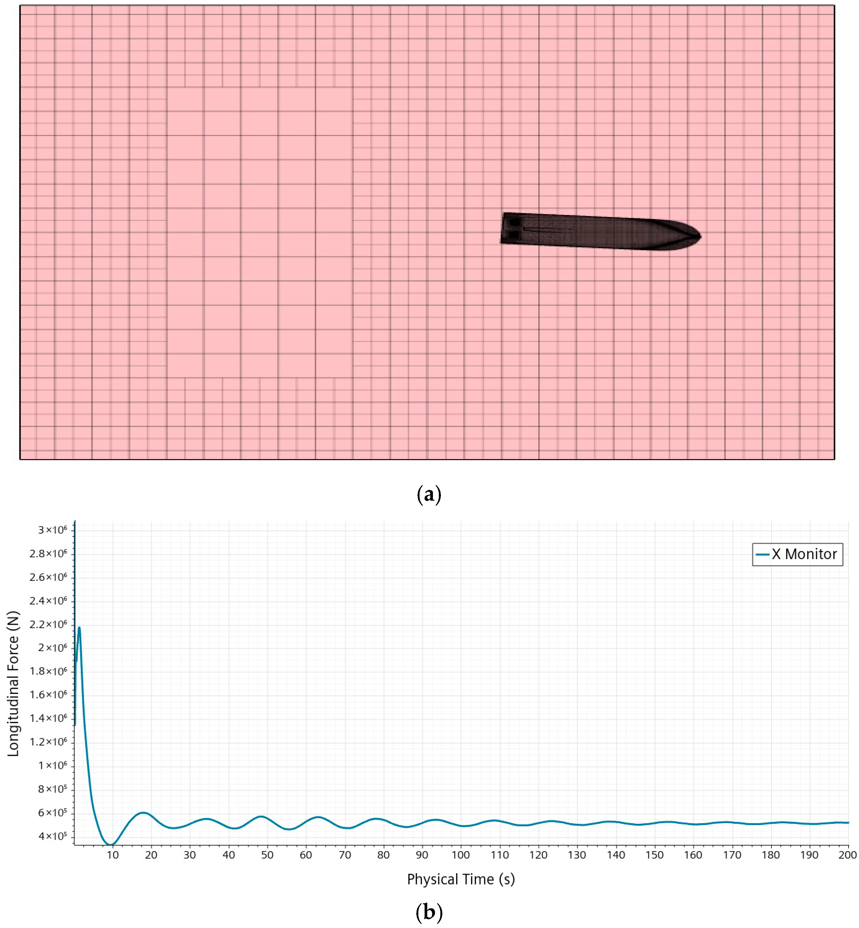
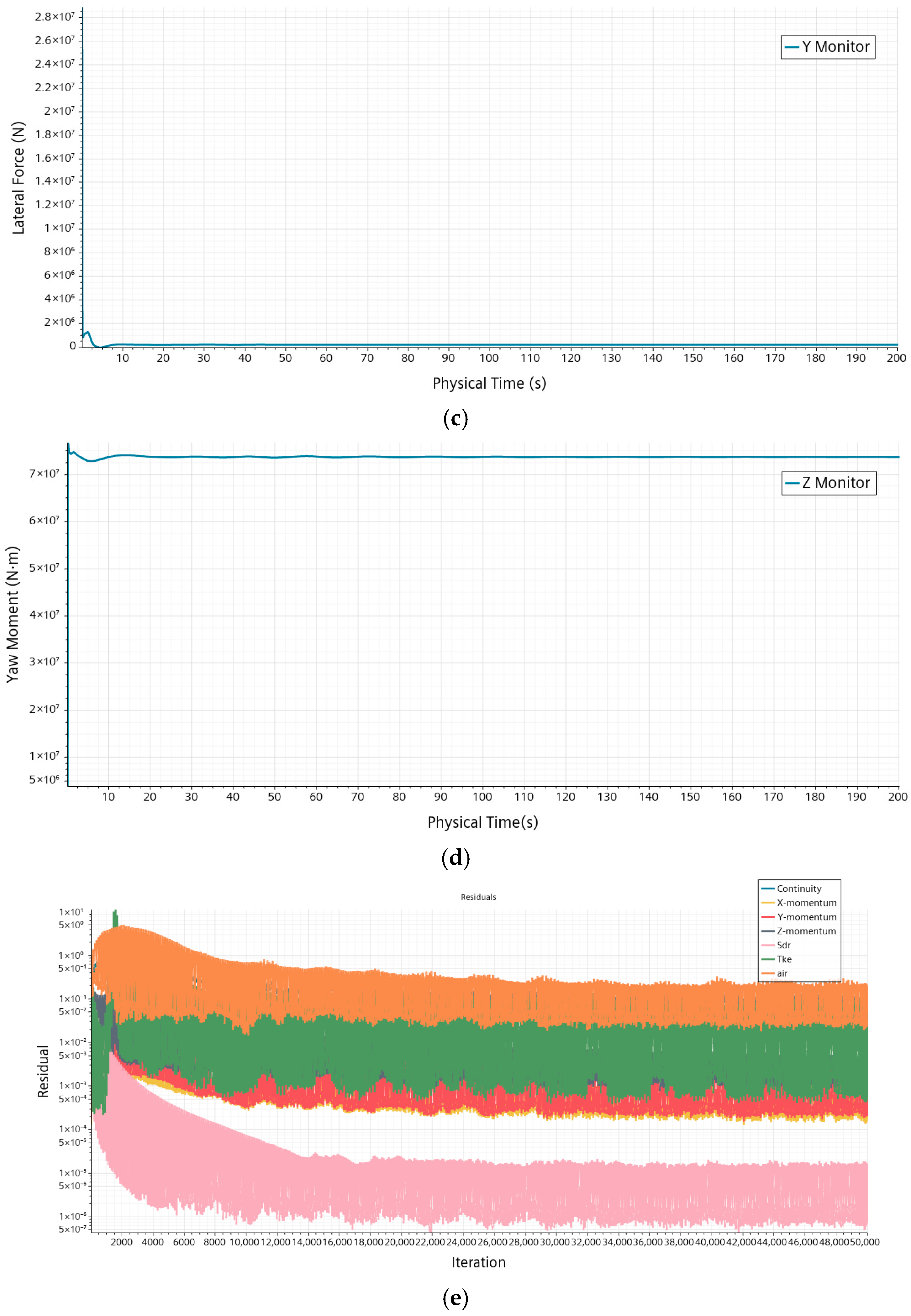
The numerical simulation was conducted on the STAR-CCM+ 2206 platform. Taking the 4° oblique navigation condition as an example, Figure 8 presents a detailed view of the ship’s heading, the computational domain mesh, as well as the computed total forces in the x and y directions and the moment about the z-axis.

Under the 4° oblique navigation condition, the variation in the force X over time is shown in Figure 8b. During the initial stage of the calculation, a significant transient fluctuation is observed, which rapidly increases to a peak of approximately 2.1 × 10⁶ N before decaying quickly. This phase primarily reflects the unsteady response of the flow field as it develops from the initial condition towards a steady state. As the simulation progresses, the force X enters an oscillatory decay stage, characterized by periodic fluctuations around the mean value with gradually decreasing amplitude. This indicates that the flow field structure is progressively establishing itself, with wake and boundary layer characteristics tending towards stability. After approximately 80 s, the X essentially reaches a steady state, with the oscillation amplitude significantly reduced. It finally stabilizes around 5.0 × 10⁵ N, exhibiting only minor periodic fluctuations. This stage indicates that the numerical calculation has largely converged, with fluctuations within 1%, confirming good stability and reliability of the obtained resistance results.

Figure 8c,d show the variations in the lateral force and yaw moment, respectively, while the computed residuals are summarized in Figure 8e. The residuals of X, Y, N are monitored to be controlled within 10⁻³, indicating that the experimental results converge well and possess credibility.

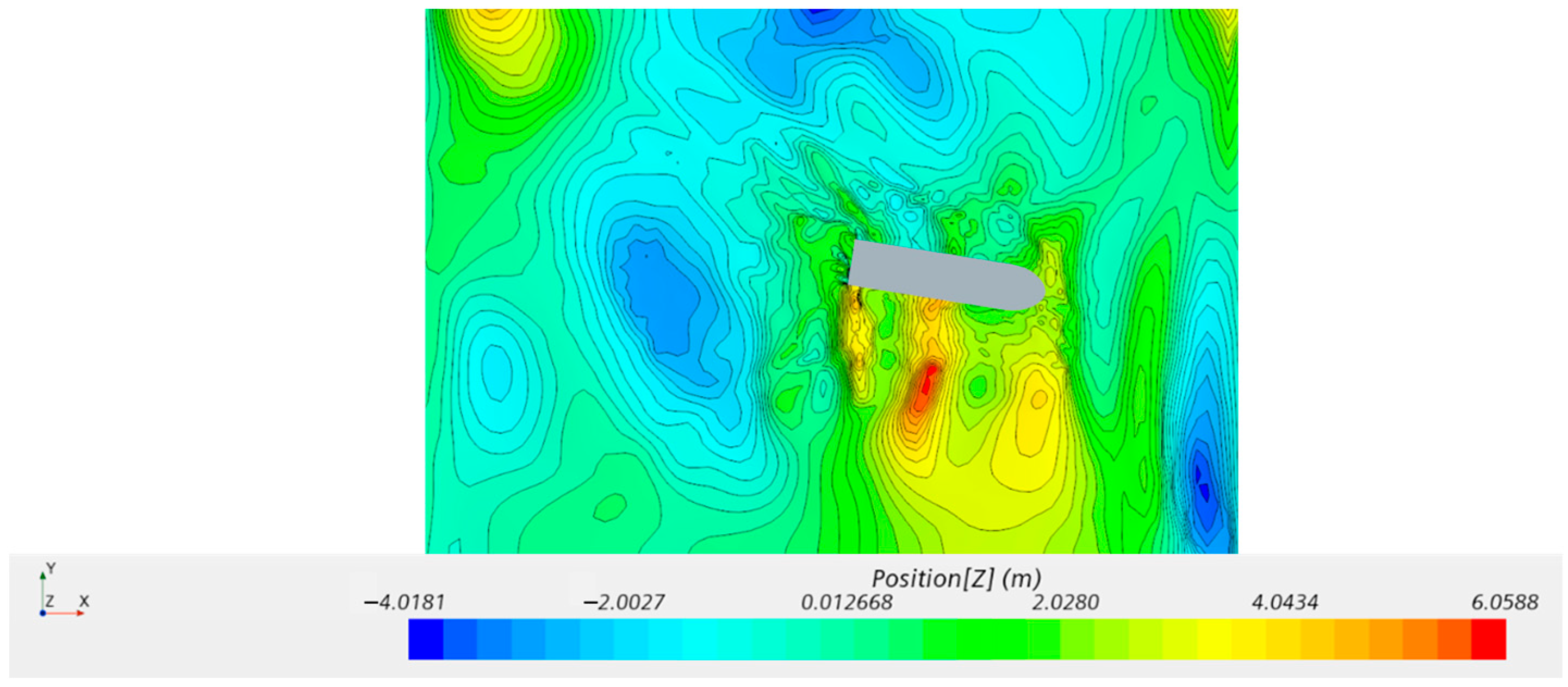
Figure 9 presents the distribution of the scalar Z in the flow field during the ship’s yaw motion. It can be clearly observed that, under the influence of the yaw angle, the flow field around the hull exhibits a notably asymmetric distribution. In the bow region, due to the angle between the incoming flow direction and the hull’s longitudinal axis, the fluid on the windward side is compressed, forming a distinct high-gradient zone, while acceleration occurs on the leeward side. Along the sides of the hull, the flow development shows significant asymmetry, especially in the mid-to-aft sections, where streamlines deflect and gradually form complex shear layer structures. In the stern and wake regions, evident flow separation and vortex structures can be observed. The yaw motion causes the wake to shift, with vortex shedding displaying directional characteristics, leading to an asymmetric distribution of vorticity in the wake area. This asymmetric wake structure further affects the lateral force and yaw moment acting on the ship. Overall, this flow field distribution reflects the significant influence of yaw motion on the flow structures around the hull. In particular, the asymmetric pressure distribution and wake deflection serve as important hydrodynamic sources contributing to the generation of lateral force and yaw moment.

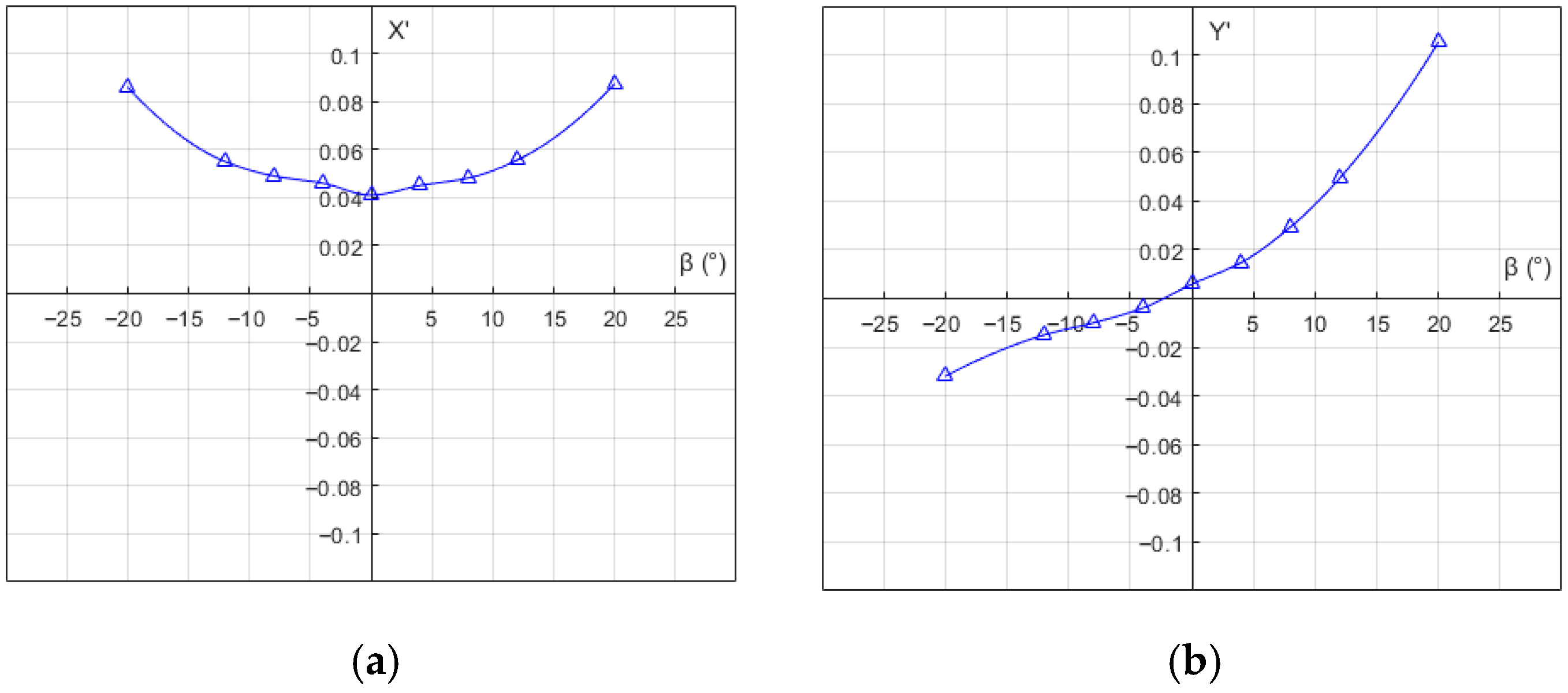
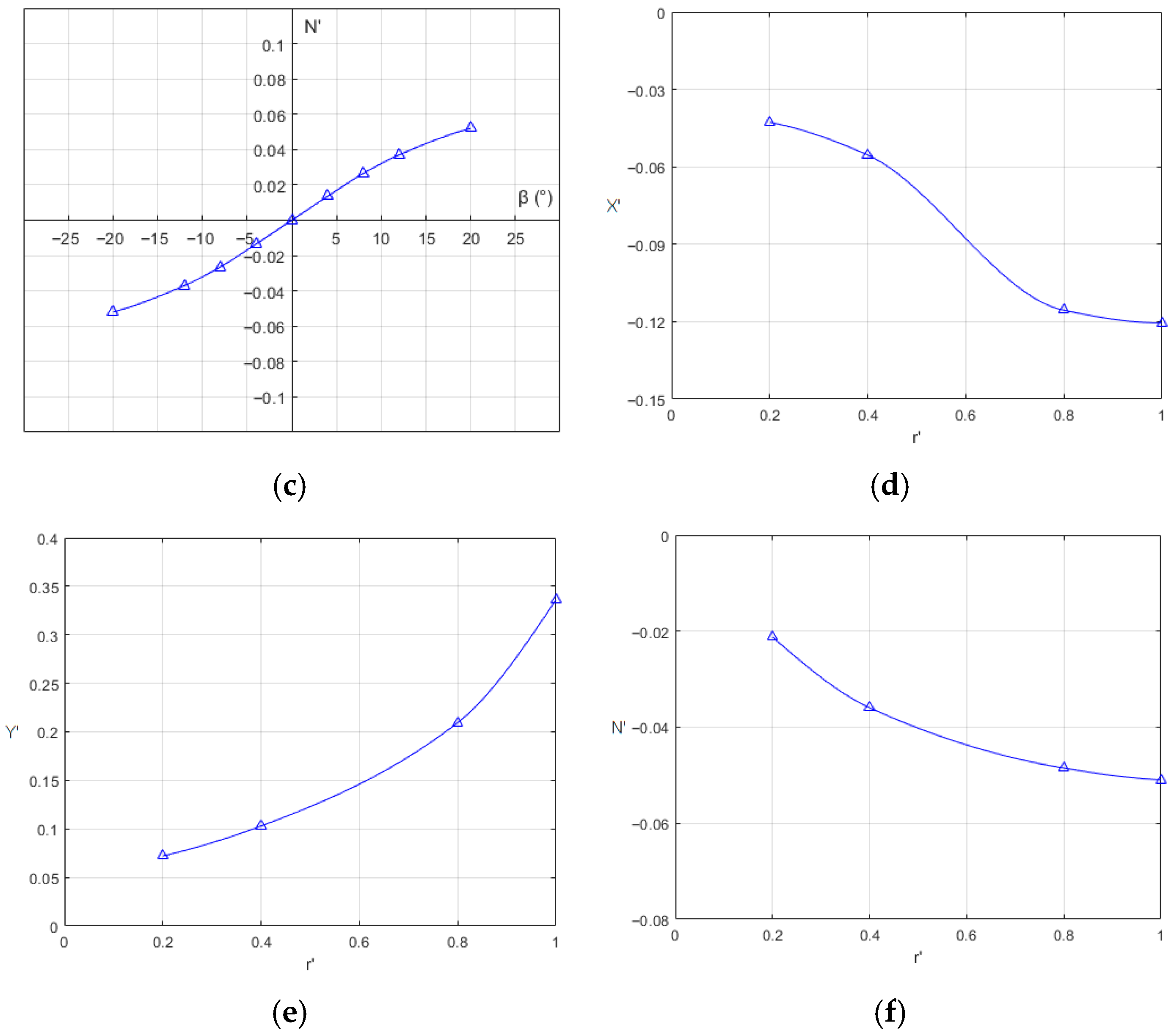
The results in Figure 10 illustrate the variation in the non-dimensionalized force X′ with respect to the drift angle β in ship maneuverability simulations. The image is symmetric about the β = 0 axis, indicating that the variation trend of X′ is similar when the ship drifts to either side. This symmetry suggests that the forces acting on the ship behave the same when the drift angle is positive or negative. The curve exhibits nonlinear characteristics, with X′ gradually increasing as β moves away from 0 in either direction. X reaches its minimum value when β = 0. This aligns with physical intuition, as the ship typically experiences the least resistance or lateral force when there is no lateral drift. The value of X′ generally lies between 0.01 and 0.1, with a slight negative value appearing near β = 0. This indicates that depending on the drift angle, the force may either assist or resist the ship’s motion. Practical Significance: This type of curve is crucial for understanding how a ship responds to different drift angles. For example, during maneuvers, the force X′ generated when the ship drifts at a certain angle can help correct the ship’s course or exacerbate the drift, depending on the direction and magnitude of the drift angle.

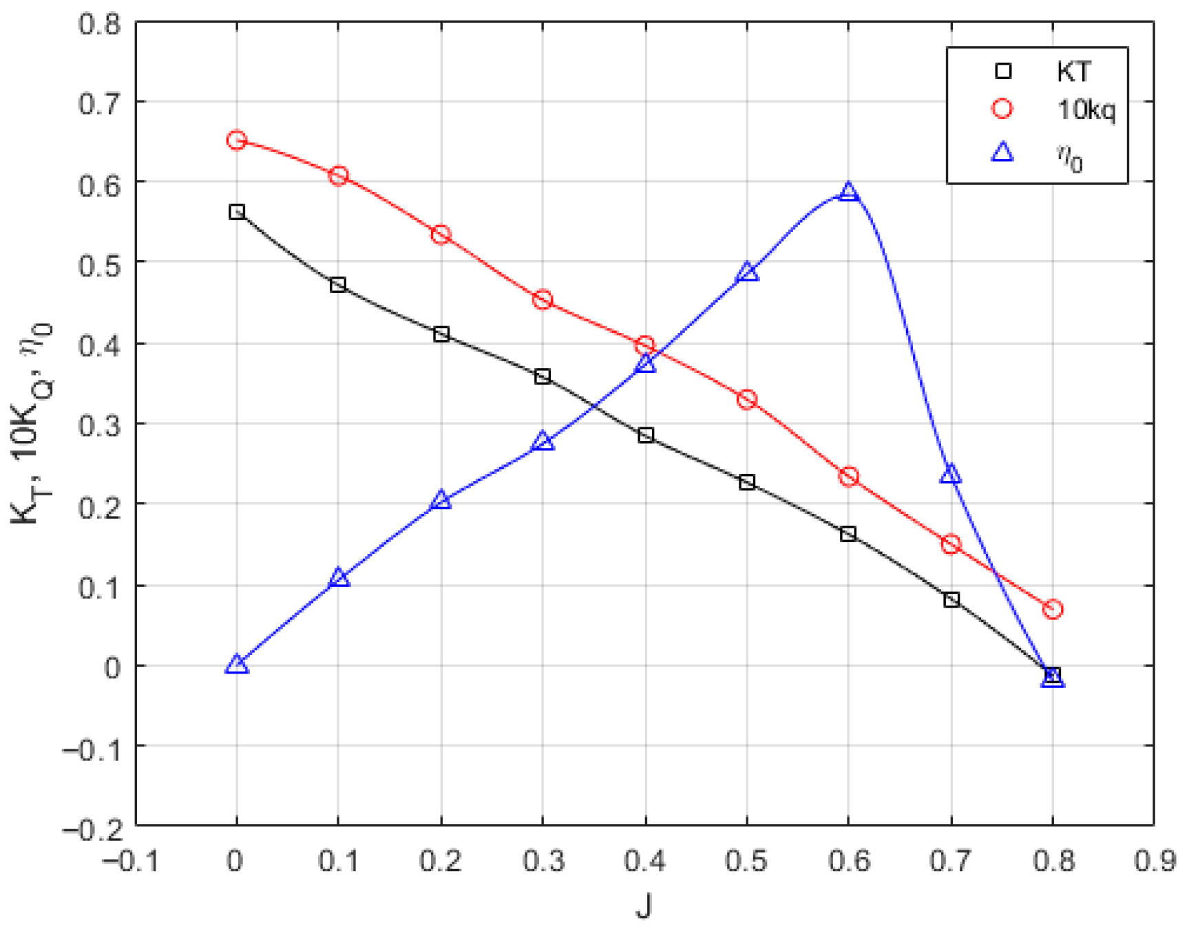
The curves of open-water characteristics of a propeller are demonstrated in Figure 11 which is typically used to analyze the performance of a propeller in free-flowing water. The thrust coefficient $K_T$ (black square markers) represents the ratio of the thrust generated by the propeller to the square of the inflow velocity and the fourth power of the propeller diameter. As the advance ratio J increases, the thrust coefficient $K_T$ gradually decreases, indicating that the propeller’s thrust efficiency declines at higher advance ratios. Torque Coefficient ${10 K}_Q$ (red circle markers) reflects the ratio of the torque produced by the propeller to the square of the inflow velocity and the fifth power of the propeller diameter. The torque coefficient also decreases with increasing J, but the rate of decrease is slower compared to the thrust coefficient. Propeller efficiency η₀ (blue triangle markers) represents the propeller’s propulsion efficiency, defined as the ratio of thrust power to shaft power. The propeller efficiency reaches its maximum within a certain range of the advance ratio and then declines as J continues to increase.

After non-dimensionalization, Equation (3) can be written as Equation (14):

$$\left\{\begin{array}{l}{X}_H^{\prime }=R_0^{\prime }+X_u^{\prime }\Delta u^{\prime }\hfill \\ Y_H^{\prime }=Y_v^{\prime }{v}^{\prime }+Y_r^{\prime }{r}^{\prime }\hfill \\ N_H^{\prime }=N_v^{\prime }{v}^{\prime }+N_r^{\prime }{r}^{\prime }\hfill \end{array}\right.$$

(14)

The obtained hydrodynamic derivatives and other factors of hull and propellers are summarized in

Table 4. Hydrodynamic derivatives of the hull.

Parameter	Value	Parameter	Value	Parameter	Value
$R_0^{\prime }$	−0.0310	$Y_v^{\prime }$	−0.1959	$N_v^{\prime }$	−0.1952
$X_u^{\prime }$	−0.024	$Y_r^{\prime }$	0.2377	$N_r^{\prime }$	0.0617

and

Table 5. Parameters of the propellers.

Parameter	Value	Parameter	Value	Parameter	Value
$K_{T{P}_0}$	0.5470	$x_p$ (m)	−37.390	rpm	179
$K_{T{S}_0}$	0.5460	$t_p$	0.193	Iz (kg·m2)	1.788 × 105
$K_{T{P}_1}$	−0.6032	$y_p$ (m)	±4.303	$z_p$ (m)	4.971
$K_{T{S}_1}$	−0.6013	${\omega }_T$	0.185
$K_{T{P}_2}$	−0.1006	$K_{T{S}_2}$	−0.1236

.

The process for identifying the derivatives involved systematic regression analysis:

(1) For small-amplitude motions, the relationship between force/moment and motion parameters is approximately linear. For instance, the linear sway derivative Y_v′ was determined by performing a linear least-squares regression on the non-dimensional lateral force Y′ plotted against the non-dimensional sway velocity v′ from the oblique towing tests at small drift angles (β = ±4°, ±8°). The coefficient of determination (R²) for this fit exceeded 0.98, confirming a strong linear correlation in this regime.

(2) For the complete model including nonlinear and coupling terms, a multivariate least-squares regression was performed. All data points from the pure yaw PMM tests—which provide combined variations in v′ and r′ at different amplitudes and frequencies—were compiled. The derivatives were obtained by minimizing the sum of squared residuals between the CFD-calculated forces/moments and the values predicted by the mathematical model. The goodness of fit for the final model with coupling terms was assessed, yielding a satisfactory root mean square error (RMSE), which validated the significance of the identified higher-order terms.

The propeller open-water characteristics (thrust coefficient K_T, torque coefficient 10 K_Q, and efficiency η₀) were obtained from simulations across a range of advance ratios (J = 0.1 to 0.8), as shown in Figure 11.

4. Maneuvering Simulations and Comparison with Full-Scale Trials

The hydrodynamic derivatives and propeller coefficients obtained from the CFD-based captive model tests were implemented within the MMG mathematical model in MATLAB R2021b to conduct virtual maneuvering simulations, specifically turning circle tests. Corresponding full-scale sea trials were performed on the vessel “Hai Yang Shi You 661”. This section presents the simulation results and compares them with the full-scale data.

4.1. Simulation Results with Different Hydrodynamic Models of Hull

Three sets of maneuvering simulations were conducted by sequentially integrating hydrodynamic models of increasing fidelity into the MMG framework:

Model 1: Linear Derivatives Only (using derivatives from Table 4, Equation (14), result in

Table 6. Comparison of simulated and tested turning circle diameters (Model 1).

Turning Angle (°)	Simulated Diameter (/L)	Tested Diameter (/L)	Relative Error (%)
15	2.9	3.5	17.1
10	4.6	4.2	9.5
5	7.7	6.1	26.2
−5	8.4	6.8	23.5
−10	5.5	4.7	17
−15	3.1	3.6	13.9

)

Model 2: Linear + Nonlinear (Uncoupled) Derivatives (using derivatives from

Table 7. Hydrodynamic derivatives of the hull (Model 2) including nonlinear terms.

Parameter	Value	Parameter	Value	Parameter	Value
$X_u^{\prime }$	−0.024	$Y_v^{\prime }$	−0.1959	$N_v^{\prime }$	−0.1952
$X_{uu}^{\prime }$	0.016	$Y_r^{\prime }$	0.2377	$N_r^{\prime }$	0.0617
$X_{vv}^{\prime }$	−0.0761	$Y_{vvv}^{\prime }$	−0.0956	$N_{vvv}^{\prime }$	0.3693
$X_{vvvv}^{\prime }$	0.2425	$Y_{rrr}^{\prime }$	0.1064	$N_{rrr}^{\prime }$	−0.044

, Equation (16), result in

Table 8. Comparison of simulated and tested turning circle diameters (Model 2).

Turning Angle (°)	Simulated Diameter (/L)	Tested Diameter (/L)	Relative Error (%)
15	2.8	3.5	20
10	3.3	4.2	21.4
5	7.6	6.1	24.6
−5	7.7	6.8	13.2
−10	3.9	4.7	17
−15	2.6	3.6	27.8

)

Model 3: Linear + Nonlinear + Coupling Derivatives (using derivatives from

Table 9. Hydrodynamic derivatives of the hull (Model 3) including coupling terms.

Parameter	Value	Parameter	Value	Parameter	Value
$X_u^{\prime }$	−0.024	$Y_v^{\prime }$	−0.1959	$N_v^{\prime }$	−0.1952
$X_{uu}^{\prime }$	0.016	$Y_r^{\prime }$	0.2377	$N_r^{\prime }$	0.0617
$X_{vv}^{\prime }$	−0.0761	$Y_{vvv}^{\prime }$	−0.0956	$N_{vvv}^{\prime }$	0.3693
$X_{vvvv}^{\prime }$	0.2425	$Y_{rrr}^{\prime }$	0.1064	$N_{rrr}^{\prime }$	−0.044
$X_{vr}^{\prime }$	−0.1826	$Y_{vrr}^{\prime }$	0.5288	$N_{vrr}^{\prime }$	0.3286
$X_{rr}^{\prime }$	0.1107	$Y_{rrr}^{\prime }$	0.1064	$N_{rrr}^{\prime }$	−0.044

, Equation (18), result in

Table 10. Comparison of simulated and tested turning circle diameters (Model 3).

Turning Angle (°)	Simulated Diameter (/L)	Tested Diameter (/L)	Relative Error (%)
15	3.4	3.5	2.9
10	3.8	4.2	9.5
5	6.8	6.1	11.5
−5	7.6	6.8	11.8
−10	5	4.7	6.4
−15	3.2	3.6	11.1

)

The quantitative comparison of the predicted tactical diameters against the tested values is summarized in the tables below. The relative error is defined as Equation (15):

$$E=\left|{\displaystyle \frac{X_{\mathrm{sim}}-X_{\mathrm{free}}}{X_{\mathrm{free}}}}\right|\times 100\%$$

(15)

All the results obtained from the tests in Star-CCM+ 2206 platform were processed in MATLAB R2021b to carry out the turning circle tests and zigzag tests. The same tests were also finished with the full-scale ship and trajectory diagrams were compared.

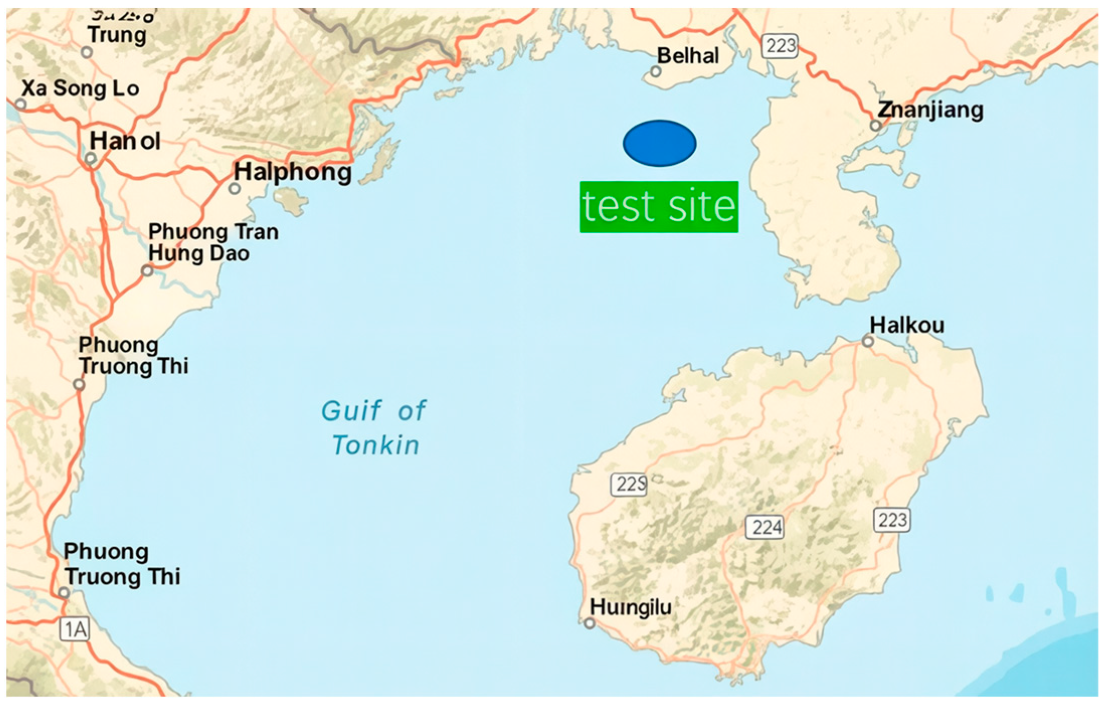
The full-scale ship turning circle test was conducted in the sea area northwest of Hainan Island in the South China Sea, where the water depth ranges between 35 and 45 m. During the test, environmental conditions included a uniform current of approximately 1 m/s and a Beaufort force 3 wind (wind speed about 4.5 m/s). The propeller maintained a constant rotational speed of 179 rpm throughout the entire experiment. The location of the test area is shown in Figure 12.

During the test, for safety considerations, the maximum rudder angle was limited to 15 degrees. Specifically, turning circle tests were performed at rudder angles of 5, 10, and 15 degrees. This limitation was implemented because significant hull heeling was observed during high-speed maneuvers with large rudder angles. The full-scale turning circle test was repeated three times, with a standard deviation within 3%. The average of these three trials was taken as the final result of the full-scale experiment.

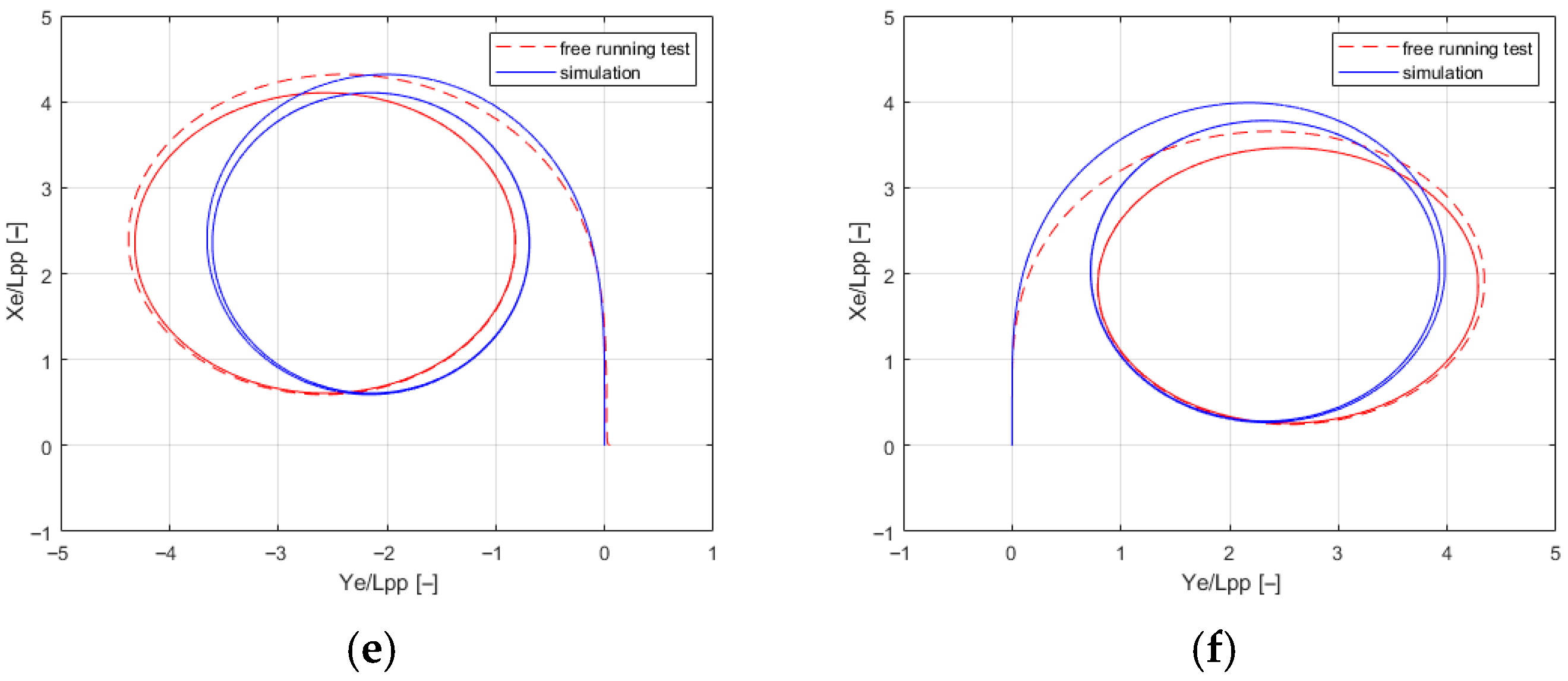
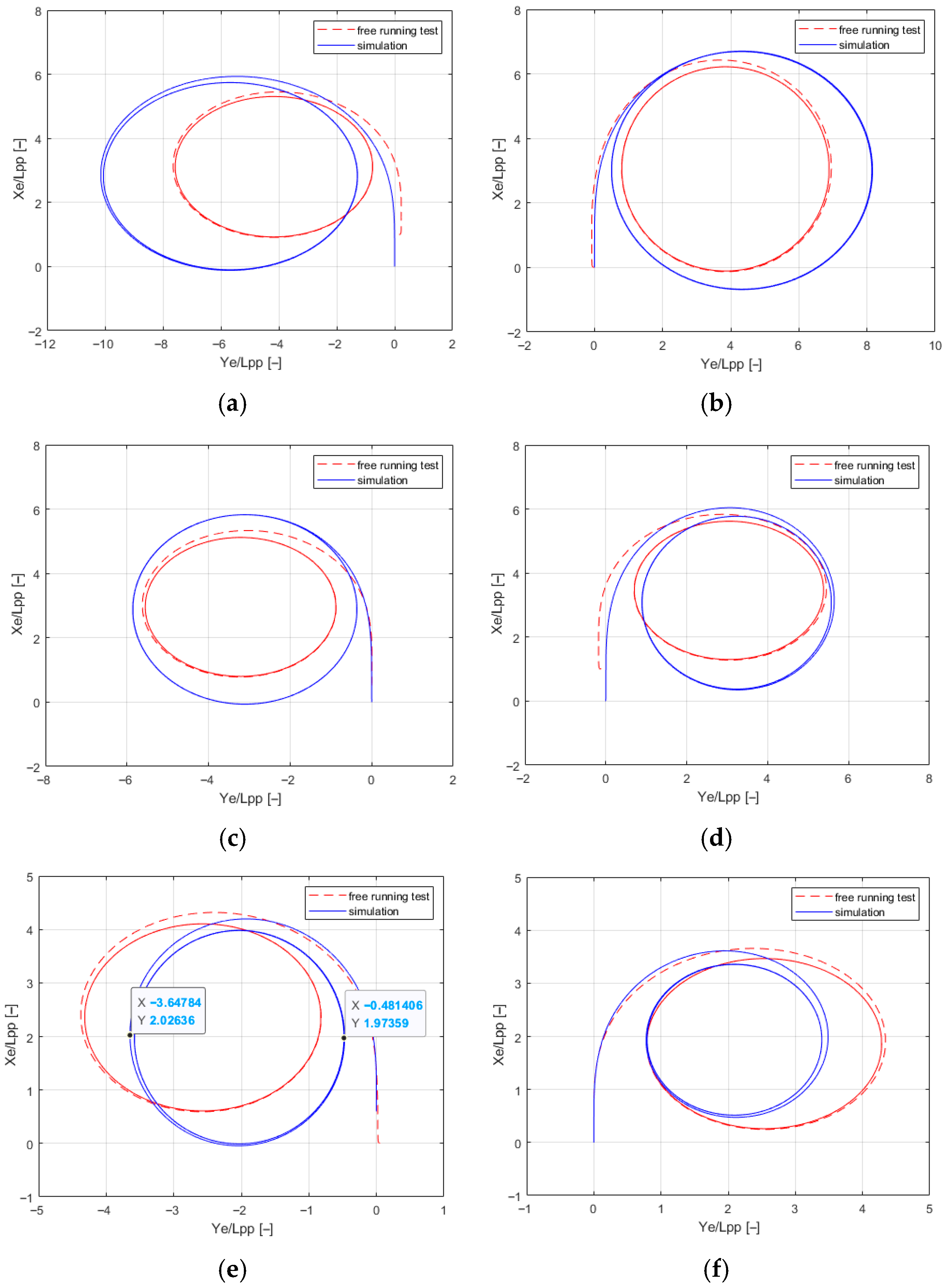
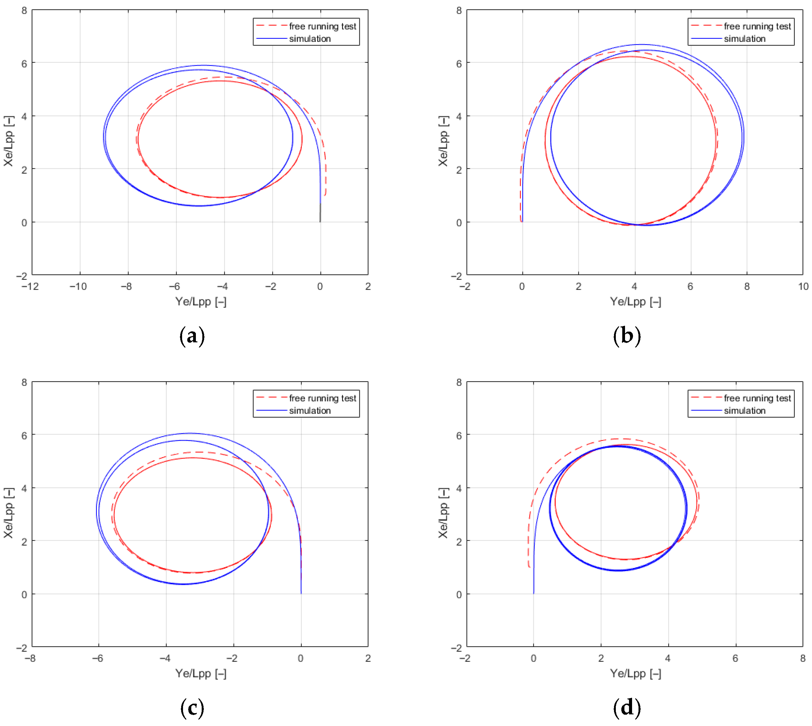
The turning circle test is typically used to assess a ship’s maneuverability under a specific rudder angle. A larger turning radius may indicate a slower response of the ship, while a smaller turning radius suggests a more responsive reaction to rudder commands. Numerical simulations (blue solid line) show relatively regular large circular trajectory in Figure 13. This shape indicates that under the simulation assumptions, the ship can maintain a relatively stable and continuous rotation at a fixed rudder angle. In the experimental setup, the superstructure was disregarded to simplify the simulation, causing discrepancies in force measurements relative to actual ship behavior. As the rudder angle increases, the ship’s turning diameter decreases, while the simulated turning diameter in the simulation decreases even faster. Comparative analysis of port and starboard experiments indicates superior agreement between the simulated and actual ship curves on the starboard side, while more discrepancies were observed on the port side. This divergence may be attributed to the presence of wind and current velocities in the actual marine environment during field trials.

Meanwhile, since only the linear terms were accounted for in the parameter fitting of hull forces, significant errors arose when simulating large-amplitude motions and turning motions as shown in Table 6. Therefore, nonlinear terms have subsequently been incorporated into the parameter fitting to examine their impact on the simulation in Equation (16). Linear derivatives (such as ${ X}_u$ and ${ Y}_v$) describe the linear effects of motion parameters (such as velocity) on forces, forming the foundation of the model. Nonlinear derivatives (such as ${ X}_{\mathit{uu}}$ and ${ Y}_{\mathit{vv}}$) capture the impact of nonlinear factors, such as the square of velocity, on forces, which become significant at high speeds or large angles of rotation. The related derivatives are shown in Table 7.

$$\left\{\begin{array}{l}{X}_H^{\prime }=X_u^{\prime }{u}^{\prime }+X_{uu}^{\prime }{u}^{\prime 2}+X_{vv}^{\prime }{v}^{\prime 2}+X_{vvvv}^{\prime }{v}^{\prime 4}\hfill \\ Y_H^{\prime }=Y_v^{\prime }{v}^{\prime }+Y_{r^{\prime }}^{\prime }{r}^{\prime }+Y_{vvv}^{\prime }{v}^{\prime 3}+Y_{rrr}^{\prime }{r}^{\prime 3}\hfill \\ N_H^{\prime }=N_v^{\prime }{v}^{\prime }+N_{r^{\prime }}^{\prime }{r}^{\prime }+N_{vvv}^{\prime }{v}^{\prime 3}+N_{rrr}^{\prime }{r}^{\prime 3}\hfill \end{array}\right.$$

(16)

Figure 14 and Table 8 present the turning circle diameters predicted by Model 2 (which includes linear and nonlinear uncoupled terms) compared against full-scale trial data for both port and starboard turns at rudder angles of 5°, 10°, and 15°. The results show that simulated diameters are consistently smaller than the tested values in all cases except starboard 5°, indicating a systematic under-prediction. Relative errors range from 13.2% to 27.8%, with an average error of approximately 20.7%. The largest error (27.8%) occurs at port 15°, compared with the linear terms, the error remained substantial. Significant port-starboard asymmetry is also observed, with error differences of up to 11.4% at the same rudder angle. However, it can be observed that the simulated turning diameters are consistently smaller than that in full-scale trials with the angles increasing. During the turning motion, significant lateral velocity (v) and yaw rate (r) are present, which can generate considerable additional resistance (speed loss). This may affect the ship’s speed during turning maneuvers.

Coupling terms are the soul of the mathematical model for ship motion, connecting independent degrees of freedom into an organic whole. In turning maneuvers, the coupling effects determine the ship’s actual turning trajectory, speed variations, and dynamic characteristics. Neglecting them makes the model only applicable to predictions under minor disturbances. When faced with real, large-amplitude maneuvering actions, significant errors inevitably arose as observed. For the planar maneuvering motion of a ship, the hydrodynamic forces on the hull are typically expressed as functions of the motion state variables: the longitudinal force X_H = X_H (u, v, r), the lateral force Y_H, and the yaw moment N_H = N_H (u, v, r). In the conventional MMG model, to facilitate engineering applications, the aforementioned nonlinear functions are typically expanded around a reference operating condition, with only the lower-order terms retained. If only the linear terms are kept, the traditional linear maneuvering model is obtained; if higher-order and cross-coupling terms are further included, a nonlinear coupled model is derived. Therefore, the mathematical origin of the coupling terms can be understood as follows: the cross-coupling terms arise naturally from the multivariate Taylor expansion of the hull hydrodynamic forces with respect to multiple motion variables. They do not reflect the contribution of a single degree of freedom, but rather the combined effect generated by the simultaneous presence of the sway velocity v and the yaw angular velocity r. From the perspective of physical mechanisms, the coupling terms are not artificially added; they are determined by the actual flow characteristics during a ship’s large-amplitude maneuvers.

(1) Sway and yaw are not independent of each other: During turning or oblique navigation, a ship typically exhibits significant sway velocity v and yaw angular velocity r simultaneously. In this situation: the sway velocity v alters the hull’s orientation relative to the incoming flow, inducing an oblique navigation effect. The yaw angular velocity r causes different local inflow velocities at various points along the ship’s length, further modifying the pressure distribution. The superposition of these two effects means that the local angle of attack and flow velocity at different parts of the hull are no longer determined by a single variable alone, but by the combined action of v and r. Consequently, the hydrodynamic forces cannot be simply expressed as a linear superposition of “sway contribution + yaw contribution”; interaction terms inevitably appear.

(2) The local inflow velocity is inherently coupled: For any point on the hull, its local transverse inflow velocity can be approximately expressed as Equation (17):

$$v_{local}=v+xr$$

(17)

where x is the position of the point relative to the center of mass.

This demonstrates that the local flow field is fundamentally determined by both the sway velocity v and the yaw angular velocity r from the outset. When nonlinear relationships exist between pressure, shear forces, or appendage loads and the local inflow velocity, cross-terms such as v²r and vr² naturally emerge after integration to obtain the total hull force and moment. In other words, coupling terms essentially originate from the integrated result of the interaction between the spatial distribution of the local velocity field and the nonlinear hydrodynamic response.

Therefore, conducting parameter fitting that includes nonlinear coupling terms in Equation (18) is an indispensable and critical step in improving the accuracy of ship motion simulations. The derivatives including coupling term are listed in Table 9.

$$\left\{\begin{array}{l}{X}_H^{\prime }=X_u^{\prime }{u}^{\prime }+X_{uu}^{\prime }{u}^{\prime 2}+X_{vv}^{\prime }{v}^{\prime 2}+X_{vvvv}^{\prime }{v}^{\prime 4}+X_{vr}^{\prime }{v}^{\prime }{r}^{\prime }+X_{rr}^{\prime }{r}^{\prime 2}\hfill \\ Y_H^{\prime }=Y_v^{\prime }{v}^{\prime }+Y_{r^{\prime }}^{\prime }{r}^{\prime }+Y_{vvv}^{\prime }{v}^{\prime 3}+Y_{vv{r}^{\prime }}^{\prime }{v}^{\prime 2}{r}^{\prime }+Y_{vr{r}^{\prime }}^{\prime }{v}^{\prime }{r}^{\prime 2}+Y_{rrr}^{\prime }{r}^{\prime 3}\hfill \\ N_H^{\prime }=N_v^{\prime }{v}^{\prime }+N_{r^{\prime }}^{\prime }{r}^{\prime }+N_{vvv}^{\prime }{v}^{\prime 3}+N_{vv{r}^{\prime }}^{\prime }{v}^{\prime 2}{r}^{\prime }+N_{vr{r}^{\prime }}^{\prime }{v}^{\prime }{r}^{\prime 2}+N_{rrr}^{\prime }{r}^{\prime 3}\hfill \end{array}\right.$$

(18)

During the experiment, a significant improvement in errors was observed, especially under large turning angle conditions. Coupling terms are crucial for simulating ship turning circle tests. Their fundamental importance lies in precisely capturing the real physical interactions of a ship during high-amplitude maneuvers. In a turning test, the ship operates in a state of strong nonlinear motion: the hull experiences a large drift angle while undergoing a rapid yaw rotation. Under these conditions, the ship’s surge, sway, and yaw motions are not independent but are tightly coupled. Significant lateral motion greatly affects the resistance (surge force) and yaw moment acting on the hull. If a mathematical model neglects these coupling terms and relies solely on linear or simple nonlinear terms for each independent degree of freedom, it fails to accurately simulate the increased drag during oblique sailing. Consequently, the model may predict a turning circle smaller than the actual one. 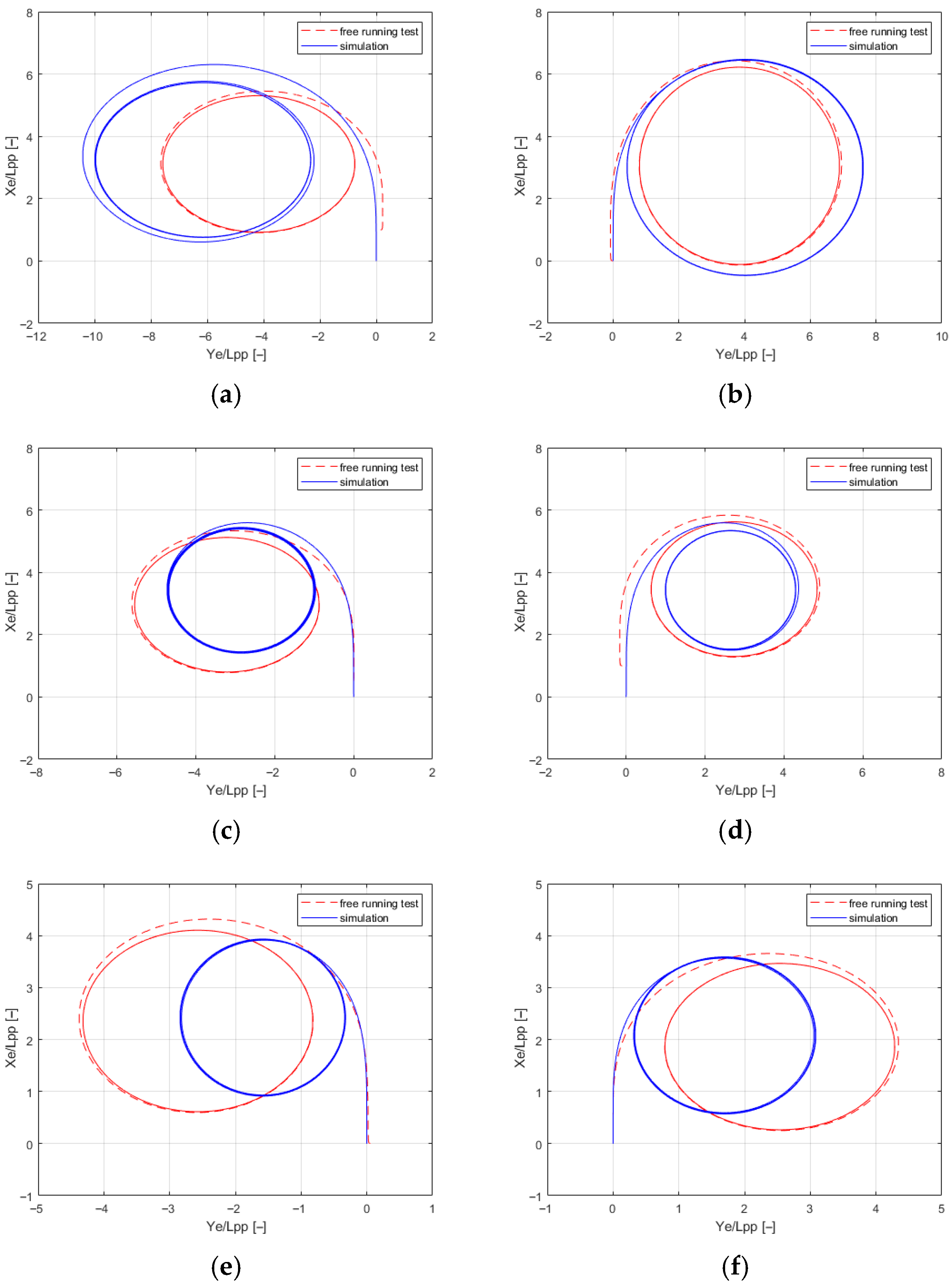As the results show in Figure 15 and Table 10, a complete model that incorporates nonlinear coupling terms can significantly reduce the prediction error for large-rudder-angle turns (for example, from over 20% to approximately 11.8%). This improvement is key to accurate engineering prediction and design evaluation.

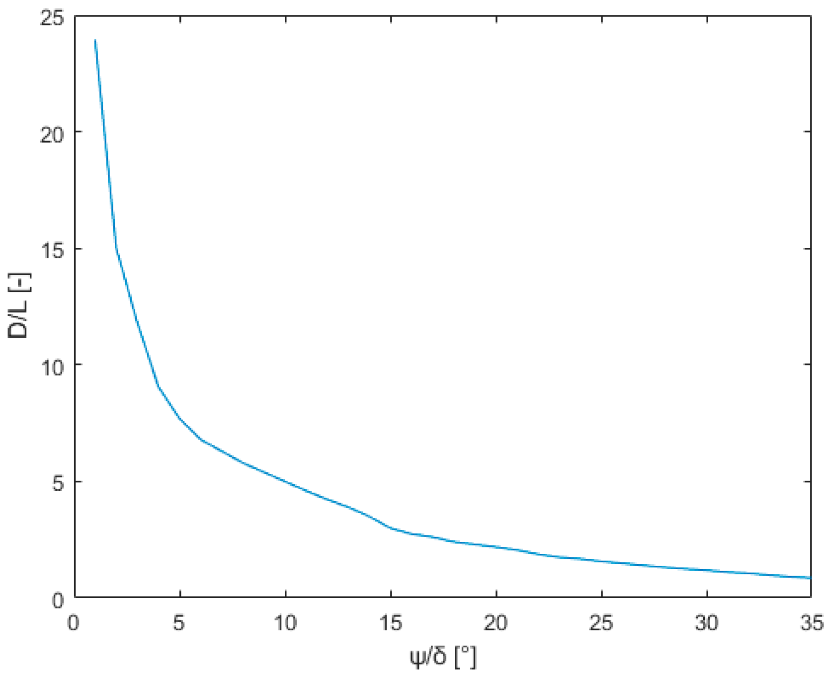
Figure 16 shows the results of the simulated turning diameters in turning maneuvers. The curve indicates that in the initial stage, the turning diameter is relatively large. As the rudder angle increases, the turning diameter decreases rapidly. After ψ reaches approximately 15° to 20°, the curve flattens considerably, meaning that further increasing the rudder angle has a diminishing effect on further reducing the turning diameter. In the free running tests, a water current speed of approximately 1 m/s and around Force 3 wind were measured, both of which exerted some influence on the experiment.

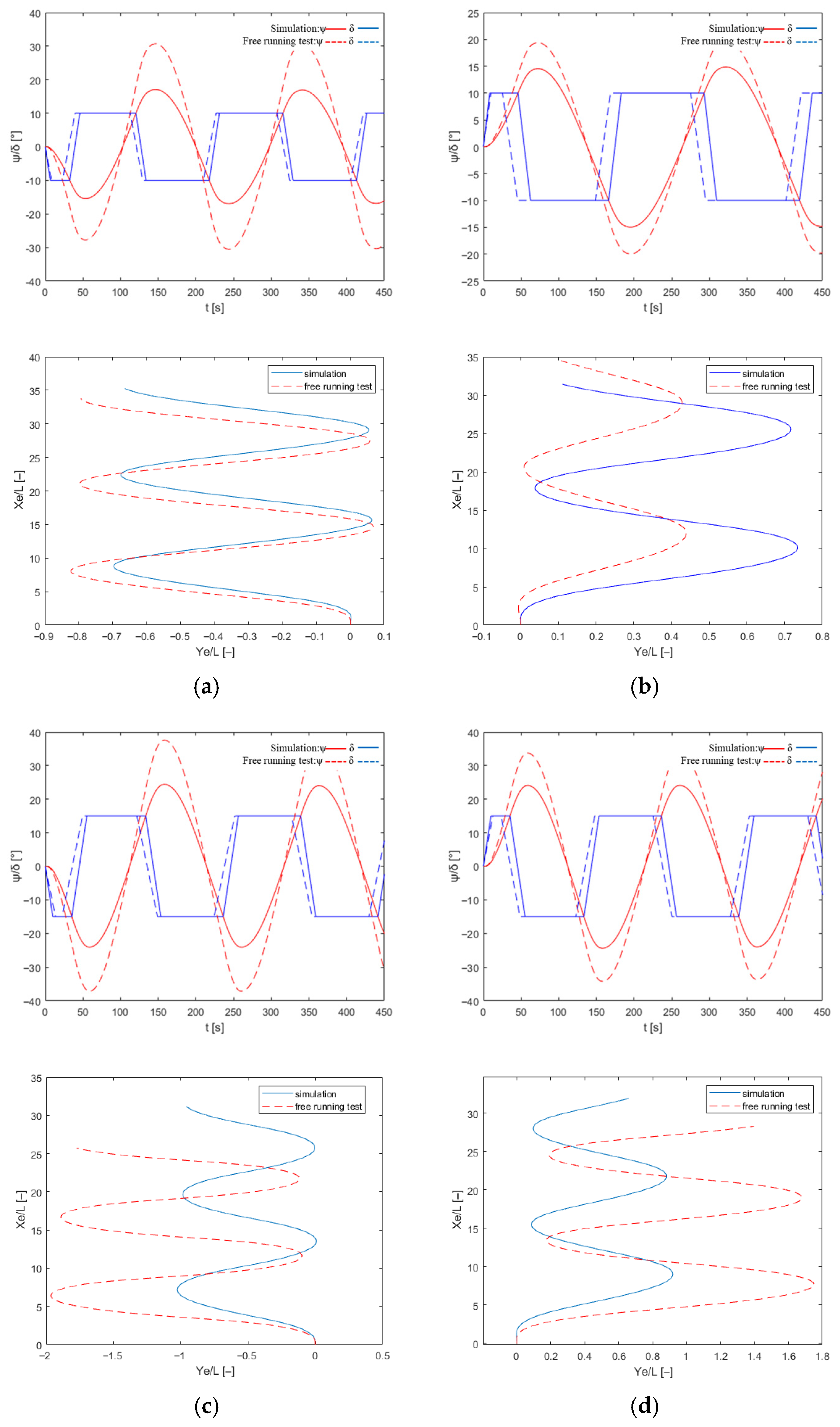
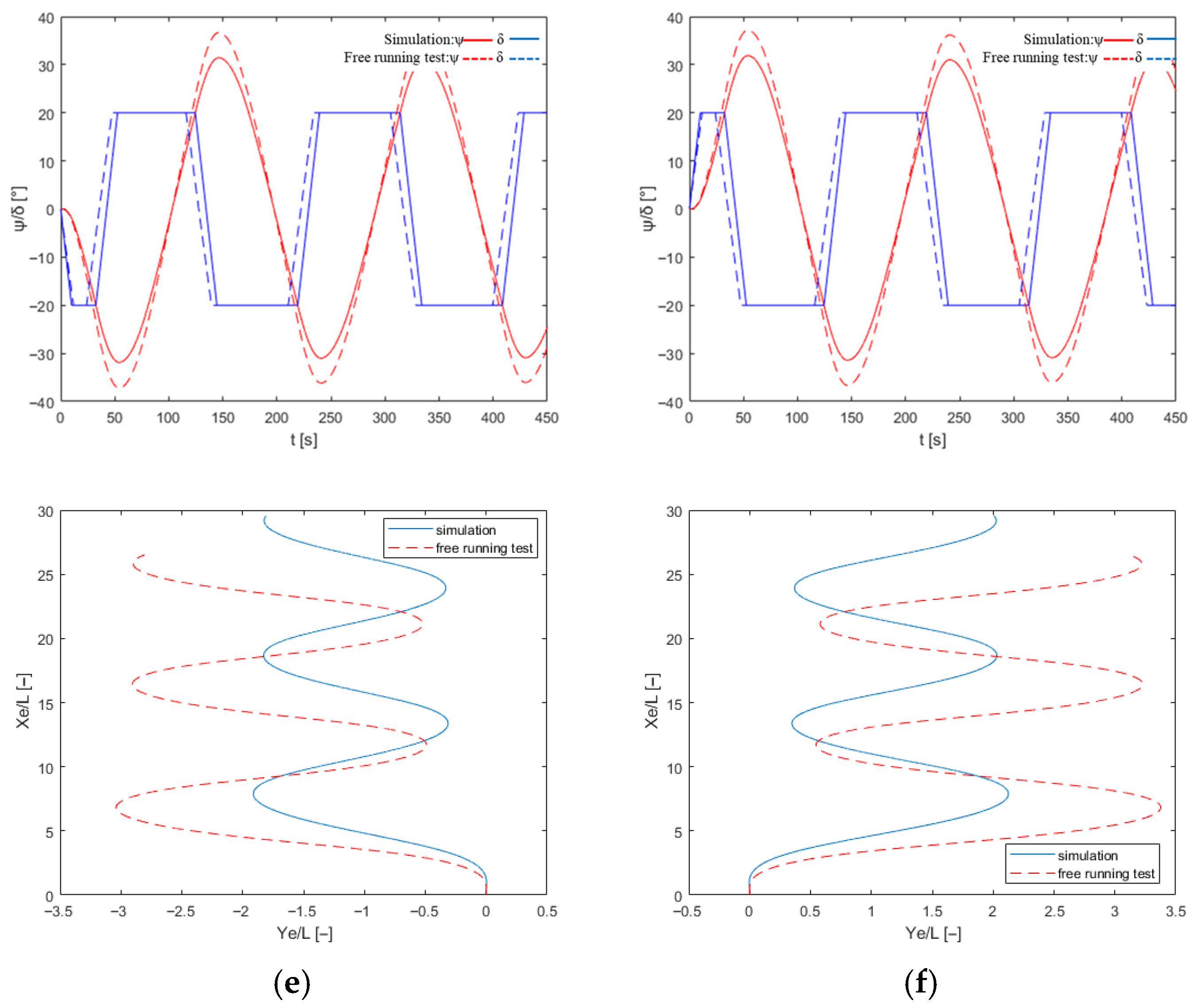
The free-running tests (red dashed line) in Figure 17 show relatively smaller and more compact trajectory, with a slight initial deviation in the opposite direction. This may reflect dynamic factors in real sea conditions, such as currents and wind, which reduce the ship’s turning radius.

Key Observations from Results

(1) Progressive Accuracy Improvement: The prediction accuracy generally improves as the model fidelity increases from Model 1 to Model 3. The Full Coupled Model (Model 3) delivers the best overall agreement with full-scale data, with most errors controlled within 11.8%.

(2) Systematic Under-prediction: A consistent trend across all models is that the simulated turning diameters are generally smaller than those measured in full-scale trials.

(3) Port-Starboard Asymmetry: For certain angles (notably 10°), the error differs between port and starboard turns, with the linear model showing a particularly large discrepancy for the starboard turn.

4.2. Analysis and Discussion of Observed Discrepancies

The results presented in Section 4.1 reveal systematic discrepancies and trends that warrant further analysis based on ship maneuvering principles and the limitations of the current numerical model.

4.2.1. Quantitative Analysis of Environmental Disturbances and Their Dominant Effects

The full-scale trials were conducted under environmental conditions including a uniform current of approximately 1 m/s and a Beaufort force 3 wind (wind speed of about 4.5 m/s), whereas both the CFD simulations and the maneuvering model were performed under ideal calm-water assumptions. This discrepancy constitutes the primary cause of the systematic positive bias observed in the results, i.e., the predicted turning diameters are generally smaller than those measured in full-scale trials.

(1) Estimation of current-induced lateral force and yaw moment:

Based on the current load formulation in Equation (19):

$$F_{\mathrm{c}}={\displaystyle \frac{1}{2}}{\rho }_w{C}_c{A}_c{U}_c^2$$

(19)

where ρ_w is the water density (1025 kg/m³), C_c is the lateral drag coefficient (typically 0.6–1.0), and A_c is the underwater lateral projected area.

The lateral projected area is estimated as:

A_c ≈ L_pp × d = 77.7 × 7.163 ≈ 556.5 m², with U_c = 1 m/s.

Thus, the current-induced lateral force is:

F_c ≈ 0.5 × 1025 × 0.8 × 556.5 × 1² ≈ 2.28 × 10⁵ N (≈228 kN).

This force acts near the center of the underwater hull, generating an additional yaw moment. Assuming a moment arm of 0.1 L_pp (~7.77 m), the current-induced yaw moment is:

N_c ≈ 2.28 × 10⁵ × 7.77 ≈ 1.77 × 10⁶ N·m (≈1.77 MN·m).

(2) Estimation of wind-induced effects:

Based on the wind load formulation in Equation (20):

$$F_w={\displaystyle \frac{1}{2}}{\rho }_a{C}_w{A}_w{U}_w^2$$

(20)

where ρ_a is the air density (1.225 kg/m³), C_w is the wind coefficient (taken as 1.0), A_w is the above-water lateral projected area (~300 m²), and U_w is the wind speed (4.5 m/s).

Thus, the wind-induced lateral force is:

F_w ≈ 0.5 × 1.225 × 1.0 × 300 × 4.5² ≈ 3.72 × 10³ N (≈3.7 kN).

Assuming a moment arm of 8.6 m, the wind-induced yaw moment is:

N_w ≈ 3.72 × 10³ × 8.6 ≈ 3.2 × 10⁴ Nm (≈32 N·m).

(3) Comparative analysis:

The magnitude of current-induced loads (~228 kN, ~1.77 MN·m) is nearly two orders of magnitude larger than that of wind loads (~3.7 kN, ~32 kN·m). In steady turning motion, a uniform current effectively introduces an equivalent constant drift angle, significantly increasing the oblique resistance and yaw damping. This is the fundamental physical mechanism leading to larger turning diameters in full-scale trials compared to calm-water simulations. Although the wind effect is smaller, it contributes to port–starboard asymmetry. Therefore, environmental current is identified as the dominant unmodeled error source, accounting for a major portion of the residual discrepancy.

4.2.2. Systematic Bias Introduced by Model Simplifications

The present framework involves necessary geometric and physical simplifications, which inevitably introduce systematic bias.

(1) Geometric simplification: In the CFD simulations, superstructures, masts, and other appendages are neglected, and the azimuth thruster pods and struts are significantly simplified. While this reduces mesh size and computational cost, it leads to two consequences. First, wind loads on superstructures are neglected (although partially reflected in full-scale conditions). Second, the complex vortex structures and additional resistance generated by the thruster pods at large deflection angles are underestimated. As a result, the total resistance and energy dissipation during turning are underestimated, making the predicted trajectory more flexible (i.e., smaller turning diameter). This effect is opposite in direction to environmental current but generally smaller in magnitude.

(2) propeller model simplification: A thrust model based on open-water characteristics is adopted, assuming symmetric inflow to the twin propellers. However, in actual turning motion, the inflow conditions of the inner and outer propellers are highly asymmetric, with significant differences in advance velocity. The present model does not account for propeller–propeller interaction or rotation-induced flow asymmetry, leading to errors in thrust and lateral force estimation, particularly affecting transient responses in the initial turning stage. Meanwhile, synchronized propeller operation, due to its simplicity and intuitiveness, is suitable for straightforward scenarios such as routine cruising and straight-line navigation. However, in situations requiring high-precision positioning, complex maneuvers, energy efficiency optimization, or redundancy and fault tolerance, its limitations—such as low operational degrees of freedom and limited adaptability—become evident. In contrast, asynchronous operation, by independently controlling each propeller, can more fully exploit the potential of multi-propeller systems, making it particularly suitable for high-end applications such as Dynamic Positioning (DP), offshore engineering operations, and maneuvering in confined waters. The trend in modern ship control systems is to integrate both modes: simplifying the operational interface while employing optimized algorithm-based asynchronous thrust allocation at the underlying level, thereby achieving a balance of safety, economy, and maneuverability.

(3) Degree-of-freedom limitation: The adopted three-degree-of-freedom model (surge, sway, yaw) neglects roll motion. In high-speed, large-angle turning, significant heel occurs. Roll alters the underwater hull geometry, propeller immersion, and inflow angle, thereby affecting hydrodynamic derivatives. Neglecting roll–sway–yaw coupling may introduce errors under highly maneuvering conditions.

4.2.3. Numerical and Parameterization Errors

(1) CFD errors: Despite mesh independence verification, the turbulence model (SST k–ω) introduces inherent modeling errors in simulating strong separation and free-surface deformation. The selection of amplitude and frequency in virtual PMM tests also affects the identification of hydrodynamic derivatives, particularly for coupling and higher-order terms.

(2) Parameter identification errors: Least-squares fitting is used to identify parameters for models of different complexity. Although linear models may exhibit high R² values, they cannot capture nonlinear behavior due to structural limitations. Fully coupled models are more physically representative but are highly sensitive to the range and accuracy of sample data, especially under large drift and yaw conditions.

4.2.4. Qualitative Analysis of Error Contributions

Based on the above analysis, the error sources are summarized qualitatively in

Table 11. Qualitative analysis of error contribution.

Sources of Error	Major Influencing Factors	Influence on Turning Diameter Prediction	Relative Contribution (Qualitative)	Reducibility
Unmodeled environmental disturbances	Lateral force balance and turning damping	Significantly increases the full-scale ship’s diameter	High (Dominant)	High (environmental force models can be coupled)
Geometric and physical simplifications	Total resistance and hull-propeller interaction	Decreases the simulated diameter	Medium	Medium (high cost of refined modeling)
Propeller model simplifications	Thrust estimation and transient response	Increases or decreases, depending on the operating condition	Medium	Medium (more advanced propeller model applicable)
Parametric and numerical errors	Accuracy of hydrodynamic derivatives	Uncertain, potentially bidirectional	Low-Medium	Low (limited by method and cost)

. The residual discrepancy between the fully coupled model predictions and full-scale trial data does not originate from the CFD–MMG methodology itself, but mainly from the gap between idealized assumptions and real-world physical complexity.

The mismatch between calm-water assumptions and environmental disturbances is the dominant source of systematic positive bias (i.e., underprediction of turning diameter). Model simplifications introduce secondary systematic negative bias. The current framework demonstrates good predictive capability (~12% error) under calm-water conditions, providing an efficient tool for design-stage performance evaluation.

For application in real-time prediction or high-fidelity digital twin systems, it is necessary to incorporate environmental load models into the simulation framework and further refine the propeller model, which constitutes an important direction for future research.

5. Conclusions

This study focuses on the dual full-revolving propulsion platform supply vessel “Haiyang Shiyou 661” and systematically conducts a study integrating Computational Fluid Dynamics (CFD) with an enhanced mathematical model to address the insufficient accuracy of maneuverability prediction under large-amplitude maneuvering conditions. By establishing a complete technical chain of “mathematical modeling-numerical experiment-parameter identification-motion simulation-full-scale validation”, the main research work can be concluded as follows:

(1) A maneuverability prediction framework suitable for dual full-revolving propulsion vessels is established. Based on the MMG-separated modeling concept, a three-degree-of-freedom maneuvering motion mathematical model is developed, clearly decomposing the total hydrodynamic forces into hull forces and propeller forces. For the core of hull hydrodynamic modeling, three models of varying complexity are innovatively designed and implemented: a linear model, a nonlinear model (incorporating higher-order terms for each degree of freedom), and a fully coupled model (further introducing coupling terms between sway and yaw velocities). This progressive model design provides a foundation for subsequent quantitative analysis of the impact of different factors on prediction accuracy.

(2) High-precision parameter identification is accomplished via CFD virtual experiments. Using the STAR-CCM+ 2206 platform, systematic oblique towing tests, virtual Planar Motion Mechanism (PMM) tests, and propeller open-water performance calculations are conducted to efficiently obtain hydrodynamic responses of the hull under various motion states and propeller characteristic curves. Employing the least squares method, the full sets of hydrodynamic derivatives corresponding to the three models are successfully identified, forming a comprehensive parametric model database suitable for engineering simulation.

(3) The key role of coupling terms is quantitatively evaluated by comparing simulation results with full-scale trial data. A maneuvering motion simulation program developed in MATLAB R2021b is used to numerically simulate turning circle and zigzag tests, followed by systematic comparison with full-scale sea trial data. The results clearly demonstrate that the maximum prediction errors of the linear and nonlinear models under large-amplitude turning conditions exceed 25%. In contrast, the fully coupled model, by explicitly introducing the sway-yaw velocity coupling terms, significantly reduces the maximum prediction error to approximately 11.8%, with key condition errors controllable to around 3%. This quantitatively confirms that velocity coupling terms are the key factor determining the prediction accuracy of large-amplitude maneuvering for dual full-revolving propulsion vessels.

(4) The sources and magnitudes of prediction errors are systematically analyzed. The study indicates that, apart from model complexity, the main identifiable causes of the residual discrepancy between simulation and full-scale data are environmental wind and current disturbances (particularly current effects) during sea trials, moderate simplifications of hull and propeller geometry, and approximate treatment of complex propeller–propeller interactions. The CFD-MMG coupled framework developed in this study is methodologically validated as effective. The residual errors primarily stem from engineering simplifications and unmodeled disturbances, pointing the way for further optimization.

In summary, this study not only provides a validated, cost-effective, and efficient numerical framework for the maneuverability prediction of dual full-revolving propulsion vessels but, more importantly, offers clear quantitative guidance for balancing model complexity and prediction accuracy in engineering practice through systematic comparative study. It holds distinct reference value for the design optimization and safe operation of such special-purpose vessels.