Feasibility Analysis of Underwater Vehicle Detection Based on Homogeneous Ellipsoidal Hull Model Using Gravity Gradient

Abstract

In recent years, as underwater vehicles continue to improve their noise reduction capabilities, sonar-based detection has faced significant challenges, and non-acoustic detection has become a research focus. Gravity gradient detection, owing to its excellent concealment and anti-interference capability, is regarded as an important non-acoustic means for underwater target detection. Based on the structural characteristics of an underwater vehicle, this paper establishes a homogeneous ellipsoidal hull (HEH) model composed of two similar rotating ellipsoids. This model assumes that the mass of an underwater vehicle is completely uniformly distributed over the outer hull. Analytical formulas for the gravity anomaly and gravity gradient anomaly generated by this model are derived, and their spatial distribution characteristics are analyzed. Furthermore, based on the HEH model, the feasibility underwater vehicle detection using the vertical gravity gradient component is analyzed. Results show that when the accuracy of the gravity gradiometer reaches ${10}^{-4}$ E, the detection distance for a large underwater vehicle with a displacement of 18,750 t can reach 570 m.

1. Introduction

Underwater vehicles represent the forefront of ocean exploration and are widely employed in marine resource development, marine environmental monitoring, and deep-sea exploration [1,2,3]. With the continuous advancement of underwater vehicle technology, the detection of these vehicles has also become an important research topic. Acoustic detection is currently the predominant detection method, often used for medium- to long-range target detection [4,5]. However, with the improvement in the noise-reduction performance of underwater vehicles, the noise levels of current advanced underwater vehicles are approaching or even falling below the level of the ocean background noise. This has significantly weakened the capability of acoustic detection for underwater vehicles. Non-acoustic detection technologies, such as optical detection [6,7], magnetic anomaly detection (MAD) [8,9,10,11], and wake detection [12,13], are now drawing increasing attention from scholars.

In recent years, with the advancement of gravimetric technology, gravity anomaly detection (GAD) has been recognized as a promising technique for underwater target detection. On the one hand, gravity detection is passive, requiring no emission of signals to the external environment and thus offering excellent stealth capabilities. On the other hand, the gravitational field signal reflects the spatial distribution characteristics of matter and is an inherent property of objects, unlike acoustic or magnetic signals, which can be easily mitigated. Some studies treat underwater vehicles as point masses, focusing on inversion algorithms for underwater targets while neglecting the mass distribution of underwater vehicles [14,15,16,17,18]. Other studies emphasize simulating the gravitational field generated by underwater vehicles and analyzing the feasibility of underwater vehicle detection using gravity signals. Sun [19] modeled an underwater vehicle as a rotating ellipsoid, assuming that the entire mass was distributed on the ellipsoidal surface. Zhang [20] modeled an underwater vehicle as a three-part composite consisting of a hemisphere, a cylinder, and a cone, also assuming that the mass was entirely distributed on the hull surface. The aforementioned studies all employed geometric surface-mass models with regular shapes but failed to account for the thickness of the hull. Moreover, they required numerical integration to calculate gravity anomaly and gravity gradient anomaly, resulting in limited generalizability and poor interpretability. Wang [21] modeled an underwater vehicle as a gravitational dipole, simplifying the calculation of the anomalous gravitational field and the gravity gradient field generated by the underwater vehicle. However, this assumption regarding the mass distribution of an underwater vehicle is overly simplistic and fails to accurately describe the actual mass distribution of the vehicle.

In fact, the hull thickness of an underwater vehicle is a key structural parameter that affects the spatial distribution of mass. The surface-mass model tends to underestimate the amplitude of the gravity gradient signal near the target, leading to large errors in the theoretical calculation of the detection distance and reducing the reliability of gravity gradient detection. Compared with the surface-mass model, the homogeneous ellipsoidal hull (HEH) model that considering variable hull thickness can more accurately reflect the actual characteristics of gravity gradient signal. This paper takes variable hull thickness as the core focus, constructs the HEH model and derives its analytical formulas, thereby providing a more accurate theoretical basis for gravity gradient detection of underwater vehicles.

The remainder of this paper is organized as follows: Section 2 introduces the related work on underwater vehicle detection; Section 3 presents the HEH model; Section 4 provides case studies on several typical types of underwater vehicles; and Section 5 presents the conclusions and future prospects.

2. Related Work

2.1. Non-Acoustic Detection Methods for Underwater Vehicles

When large underwater vehicles move, they generate various detectable signals, including thermal [22], biological [23], chemical pollution [24], hydrodynamic [25], electromagnetic [26], and gravitational signatures [20] produced by their motion [27]. These methods serve as valuable complements to acoustic detection and hold significant promise. Among them, wake-based detection and MAD have received greater attention. Additionally, gravity gradient detection is an emerging and promising technology due to its high concealment and precision.

The wake generated by an underwater vehicle can persist in the ocean for several days, making the detection of such wakes feasible. Based on wake information, the size, position, and velocity of an underwater vehicle can be determined [28,29]. When an underwater vehicle is in motion, its wake region generates numerous vortices, especially when the vehicle travels at high speeds or frequently changes its speed and direction, resulting in significantly larger vortices. Typically, theoretical methods, experimental methods, and computational fluid dynamics (CFD) techniques are employed to study the wake field of an underwater vehicle in motion. However, when underwater vehicles operate at great depths or low speeds, wake phenomena can be difficult to observe on the ocean surface.

Magnetic detection technology has garnered widespread attention as a non-acoustic method for underwater target detection [26]. Most underwater vehicles are ferromagnetic. Magnetic-based underwater vehicle localization methods extract characteristic signals related to the vehicle’s position and distribution by utilizing the spatial distribution of magnetic anomaly signals generated by ferromagnetic underwater vehicles. Magnetometers can be deployed in the air, on the water surface, and underwater to achieve detection and localization of magnetic anomaly targets. They offer advantages including high positioning accuracy, strong anti-interference capability, and passivity, and are regarded as an effective non-acoustic detection method. However, MAD methods rely on the ferromagnetism of the target material. When underwater vehicles are constructed from low-magnetic materials, MAD methods become ineffective.

In recent years, some scholars have pointed out that gravity anomaly and gravity gradient anomaly can be used to detect underwater targets [20]. When an underwater vehicle is floating, the weight of the displaced water equals its own weight. Due to the uneven mass distribution, the vehicle generates an anomalous gravity gradient field in the surrounding area. GAD is passive, offering excellent concealment and independence from target motion. Furthermore, like magnetic signals, gravity signals propagate in water in the same manner as in air. Therefore, the detection of underwater vehicles using gravity anomaly and gravity gradient anomaly is regarded as an important complement to acoustic detection and holds great promise.

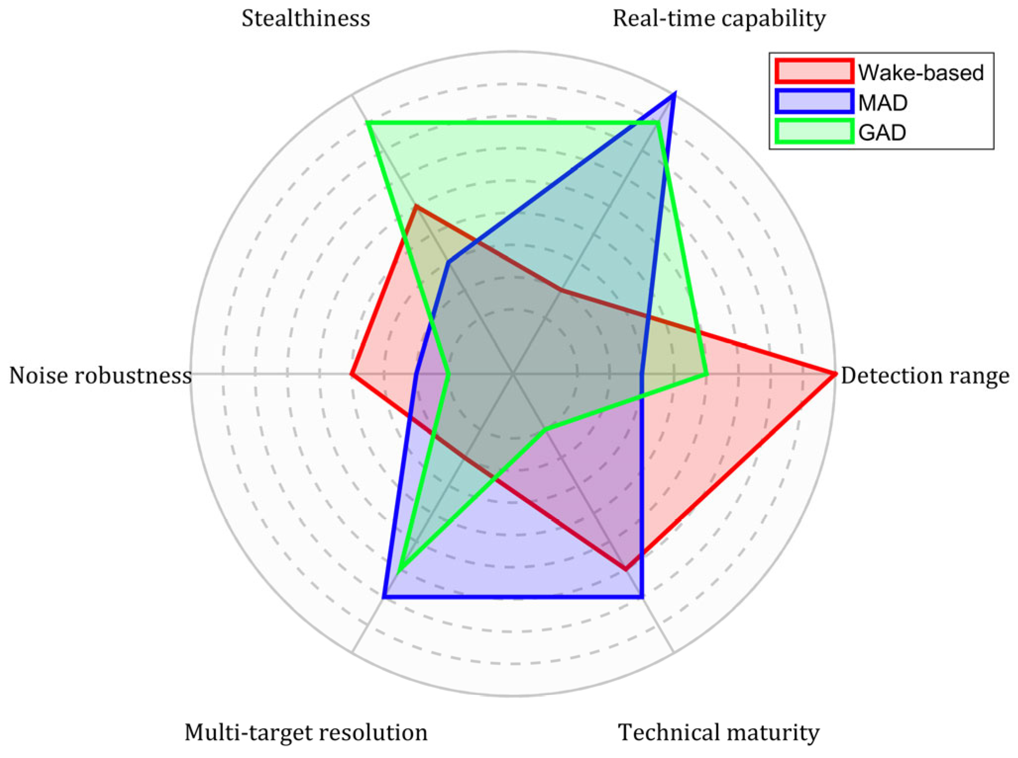
Overall, Figure 1 compares the advantages and disadvantages of three non-acoustic detection methods, namely wake-based detection, magnetic-anomaly based detection, and gravity-anomaly based detection.

2.2. Gravity Gradient Detection Models for Underwater Vehicles

At present, common GAD models mainly include particle models and geometric models. The calculation of particle models is simpler, and many researchers are focused on particle-based underwater object localization algorithms. In 2010, Wu [14,15] proposed the automated gravity gradient tensor inversion (AGTI) method for locating an underwater target, which has far-reaching implications for subsequent research. However, it requires two conditions to be met. First, the object must remain stationary for a long period of time. Second, it is necessary to extensively measure the gravity gradient anomaly around the object in order to calculate the mass through double integration. Unfortunately, when locating an underwater moving object, both of these conditions are often difficult to satisfy. In 2014, Yan [16] proposed a gravity gradient differential ratio (GGDR) method, which assumes that the object is stationary. The gravity gradiometer is mounted on an autonomous underwater vehicle (AUV), and the gravity gradient difference (GGD) and GGDR are calculated by continuously measuring the gravity gradient anomaly three times in a short period of time. The object localization problem is defined as a nonlinear problem and solved using the Newton–Raphson method. Afterwards, Yan [17] and Tang [18] proposed analytical inversion formulas (AIFs) for locating an airborne moving object by combining gravity anomaly and gravity gradient anomaly. This method also does not require large-scale measurement of gravity anomaly and gravity gradient anomaly and has high accuracy. However, the above methods assume that the target is a particle with a large excess mass. This assumption may be feasible for underwater terrain or reefs, but it does not apply to floating underwater targets, because the mass of the target is equal to the displaced water mass and there is no excess mass.

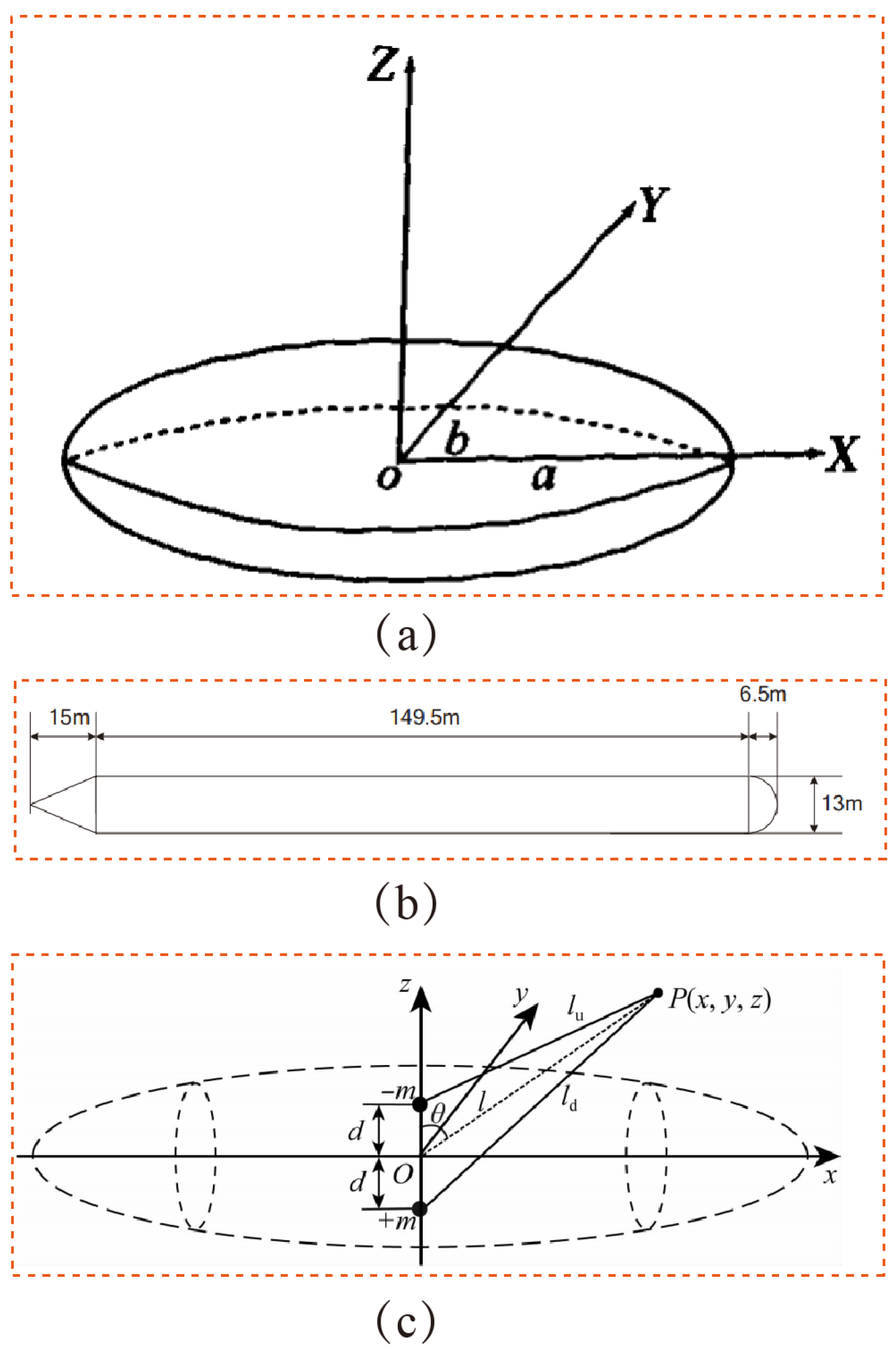
On the other hand, some studies model underwater vehicles as geometric shapes and investigate the distribution of gravity anomaly generated by underwater targets, as shown in Figure 2. In 2010, Sun [19] proposed a homogeneous ellipsoid model (HEM) to simulate an underwater vehicle, assuming that the mass is distributed on the zero-thickness outer shell of the vehicle. He calculated the gravity gradient anomaly distribution of the vehicle and pointed out that when the diving depth is 100 m, as long as the accuracy of the gravity gradiometer reaches ${10}^{-6}$ E, the detection distance can reach 1000 m. In 2018, Zhang [20] presented the three-section model (TSM), as shown in Figure 2b, still assuming that the mass is distributed on the zero-thickness outer shell, and considering the design principle that the center of buoyancy of the submarine is slightly higher than its center of gravity. In 2021, Wang [21] considered the fact that the center of buoyancy of an underwater vehicle is slightly higher than the center of gravity, and referred to the concept of magnetic dipoles to propose the gravitational dipole model (GDM), in which the upper half of an underwater vehicle is modeled as a negative-mass particle and the lower half as a positive-mass particle.

2.3. Limitation of Existing Models

Through a detailed analysis of the existing gravity gradient detection models for underwater vehicles, it can be found that these models share three common core limitations, which restrict their engineering applications. First, all models ignore the thickness of the underwater vehicle hull and assume that the mass is distributed on the hull surface or concentrated at a single point. This is inconsistent with the actual engineering structure of underwater vehicles, and the physical realism of the models is insufficient. Second, most models rely on numerical integration to calculate the gravity gradient anomaly, and only a few simplified models (such as the point mass model and the gravitational dipole model) have analytical formulas. However, these analytical formulas are overly simplified. Numerical integration has the disadvantages of low calculation efficiency and poor generalizability, and the calculation process needs to be re-established for different models. Third, the simplified mass distribution assumption leads to large systematic errors in signal calculation, which may overestimate or underestimate the gravity gradient signal amplitude and decay rate. As a result, the theoretical calculation of the detection distance becomes inconsistent with the actual engineering conditions, thereby reducing the reliability of the model.

In summary, the existing gravity gradient detection models for underwater vehicles have obvious limitations in their mass distribution assumptions and calculation methods, and there is an urgent need to establish a gravity gradient model that considers the variable thickness of the hull and has closed-form analytical formulas. Based on this, this paper proposes the HEH model with variable thickness, and conducts an in-depth investigation of its gravity gradient signal characteristics and detection feasibility.

3. Homogeneous Ellipsoidal Hull Model

Assuming that the shape of an underwater vehicle is a rotational ellipsoid described by the following equation:

$${\displaystyle \frac{x^2}{a^2}}+{\displaystyle \frac{y^2+z^2}{b^2}}=1.$$

(1)

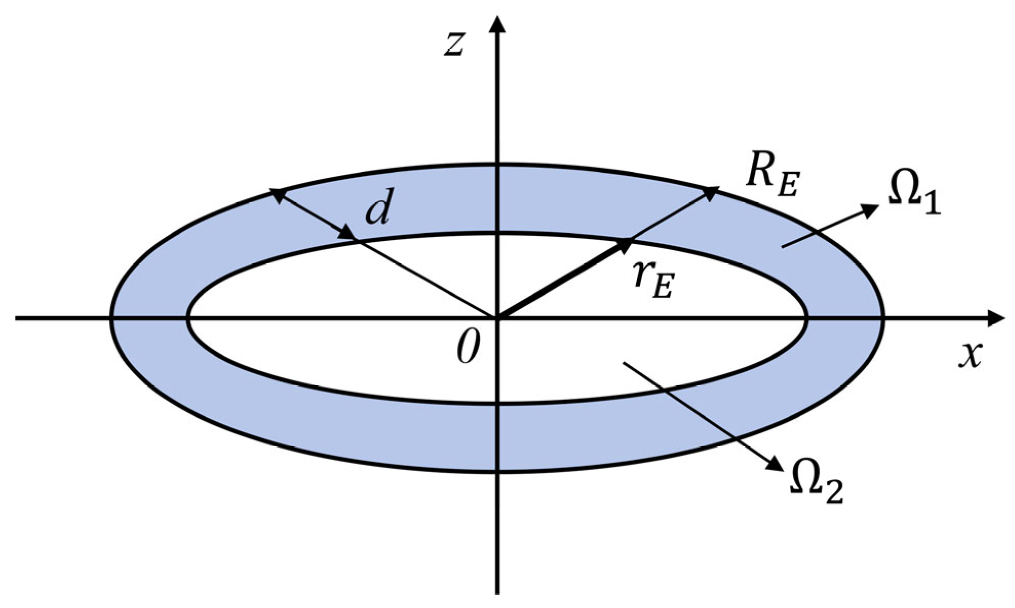
Assume that an underwater vehicle is composed of two layers, with its entire mass distributed on the outer hull ${\mathsf{\Omega }}_1$, which has a thickness of $d$ and a density of ${\rho }_h$. The inner region ${\mathsf{\Omega }}_2$ is a similar ellipsoid that shares the same origin as the outer ellipsoid and has negligible mass, as illustrated in Figure 3. The underwater displacement of the vehicle is equal to its own weight:

$$m_{\downarrow }={\rho }_w{V}_{\downarrow }={\rho }_h{V}_1,$$

(2)

where $m_{\downarrow }$ is the submerged displacement of the vehicle, ${\rho }_w$ is the density of seawater, $V_{\downarrow }={\displaystyle \frac{4}{3}}\pi a{b}^2$ is the displacement volume of the underwater vehicle, $V_1=V_{\downarrow }-V_2$ is the volume of the outer hull, $V_2={\displaystyle \frac{4}{3}}{\lambda }^3\pi a{b}^2$ is the volume of the inner region, and $\lambda \in (0, 1)$ is the similarity ratio.

Simplify Equation (2) to obtain:

$$\lambda =\sqrt[3]{1-{\rho }_w/{\rho }_h}.$$

(3)

3.1. Gravitational Potential of a Homogeneous Ellipsoid

The gravitational potential at an external point $P^{\prime }$ generated by an ellipsoid with uniform density $\rho$ can be expressed as [30]

$$V\left(P^{\prime }\right)=G\rho {\iiint }_{\mathsf{\Omega }}{\displaystyle \frac{1}{R(P,P^{\prime })}}d\mathsf{\Omega },$$

(4)

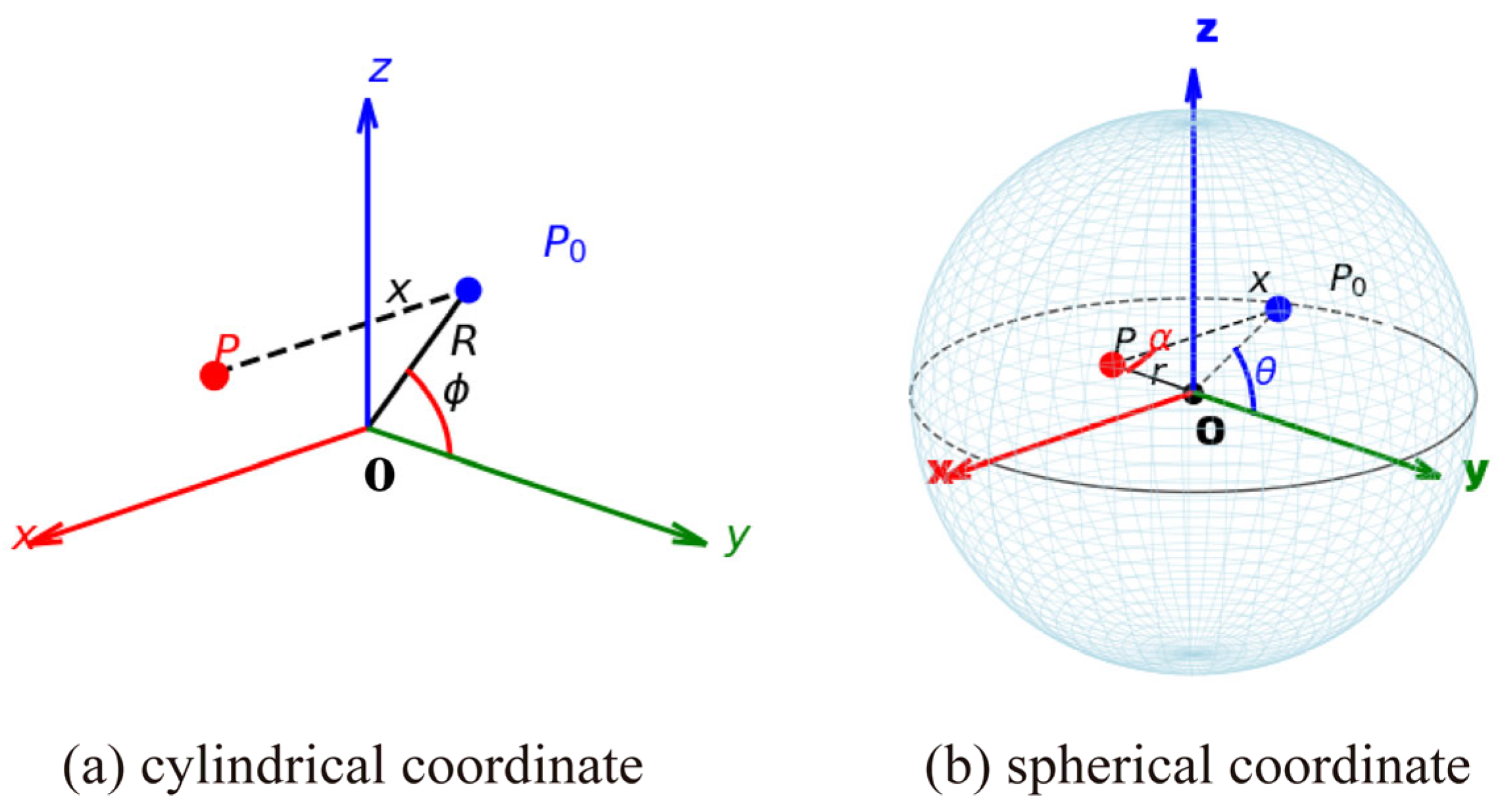
where $\mathsf{\Omega }$ represents the entire ellipsoid, $P\in \mathsf{\Omega }$ is a point within the ellipsoid, and $G$ is the gravitational constant. The distance $R(P,P^{\prime })$ between point $P$ and point $P^{\prime }$ takes different forms in different coordinate systems, as shown in Figure 4. In a Cartesian coordinate system, the distance $R(P,P^{\prime })$ between point $P(x,y,z)$ and point $P^{\prime }(x^{\prime },y^{\prime },z^{\prime })$ can be expressed as

$$R\left(P,P^{\prime }\right)=\sqrt{{(x-x^{\prime })}^2+{(y-y^{\prime })}^2+{(z-z^{\prime })}^2}.$$

(5)

In cylindrical coordinates $\left\{\begin{array}{c}x=x\\ y=R\cos \phi \\ z=R\sin \phi \end{array}\right.$, $R(P,P^{\prime })$ can be written as

$$R\left(P,P^{\prime }\right)=\sqrt{{(x-x^{\prime })}^2+R^2+{R^{\prime }}^2-2R{R}^{\prime }\cos (\phi -{\phi }^{\prime })}.$$

(6)

In spherical coordinates $\left\{\begin{array}{c}x=r\cos \alpha \\ y=r\sin \alpha \cos \theta \\ z=r\sin \alpha \sin \theta \end{array}\right.$, $R(P,P^{\prime })$ can be written as

$$R\left(P,P^{\prime }\right)=\sqrt{r^2+{r^{\prime }}^2-2r{r}^{\prime } [\cos \alpha \cos {\alpha }^{\prime }+\sin \alpha \sin {\alpha }^{\prime }\cos (\theta -{\theta }^{\prime })]}.$$

(7)

In the above three coordinate systems, the integrated volume unit element $d\mathsf{\Omega }$ is

$$\left\{\begin{array}{c}d\mathsf{\Omega }=dxdydz\\ d\mathsf{\Omega }=rdxdrd\phi \\ d\mathsf{\Omega }=r^2\sin \alpha drd\alpha d\theta \end{array}\right..$$

(8)

3.1.1. Special Case: Gravitational Potential of a Homogeneous Ellipsoid at $P^{\prime }\in x$-Axis

Firstly, we consider a point $P^{\prime }(x^{\prime },y^{\prime },z^{\prime })$ on the x-axis, where $x^{\prime }\ge a$, $y^{\prime }=z^{\prime }=0$.

We decide to calculate Equation (4) in cylindrical coordinates. In this case, $r^{\prime }=0$, thus $R(P,P^{\prime })$ can be written as

$$R\left(P,P^{\prime }\right)=\sqrt{{(x-x^{\prime })}^2+r^2}.$$

(9)

Substituting Equation (9) into Equation (4) yields

$$V\left(P^{\prime }\right)=G\rho {\int }_{-a}^{a}dx{\int }_0^{\sqrt{b^2\left(1-{\displaystyle \frac{x^2}{a^2}}\right)}}dr{\int }_0^{2\pi }{\displaystyle \frac{r}{\sqrt{{(x-x^{\prime })}^2+r^2}}}d\phi .$$

(10)

The integrand function ${\displaystyle \frac{r}{\sqrt{{(x-x^{\prime })}^2+r^2}}}$ does not contain $\phi$, therefore

$$\begin{gathered} V\left(P^{\prime }\right)=G\rho {\int }_{-a}^{a}dx{\int }_0^{\sqrt{b^2\left(1-{\displaystyle \frac{x^2}{a^2}}\right)}}dr{\int }_0^{2\pi }{\displaystyle \frac{r}{\sqrt{{\left(x-x^{\prime }\right)}^2+r^2}}}d\phi \\ =2\pi G\rho {\int }_{-a}^a\left[\sqrt{b^2+{x^{\prime }}^2+{\displaystyle \frac{a^2-b^2}{a^2}}{x}^2-2x^{\prime }x}-(x^{\prime }-x)\right]dx. \end{gathered}$$

(11)

Considering that

$$\begin{gathered} \int \sqrt{A{x}^2+Bx+C}dx={\displaystyle \frac{\left(4AC-B^2\right)\ln \left|\sqrt{A}\sqrt{A{x}^2+Bx+C}+Ax+\frac{B}{2}\right|}{8A\sqrt{A}}} \\ +\left({\displaystyle \frac{x}{2}}+{\displaystyle \frac{B}{4A}}\right)\sqrt{A{x}^2+Bx+C}+C^{\prime }, A>0. \end{gathered}$$

(12)

In Equation (11), $A={\displaystyle \frac{a^2-b^2}{a^2}}>0$, $B=-2x^{\prime }$, and $C=b^2+{x^{\prime }}^2$. Substituting Equation (12) into Equation (11) yields the closed form of the integral:

$$\begin{gathered} V\left(P^{\prime }\right)=2\pi G\rho {\int }_{-a}^a\left[\sqrt{b^2+{x^{\prime }}^2+{\displaystyle \frac{a^2-b^2}{a^2}}{x}^2-2x^{\prime }x}-\left(x^{\prime }-x\right)\right]dx \\ =2\pi G\rho \left\{-{\displaystyle \frac{a{b}^2\left({x^{\prime }}^2-E^2\right)}{2E^3}}\ln \left[1+{\displaystyle \frac{-2aE+2E^2}{\left(x^{\prime }+a\right)E-a{x}^{\prime }-E^2}}\right]+{\displaystyle \frac{a{x}^{\prime }\left(a^2+E^2\right)}{E^2}}-2a{x}^{\prime }\right\} \\ ={\displaystyle \frac{2\pi G\rho a{b}^2}{E}}\left[{\displaystyle \frac{x^{\prime }}{E}}-{\displaystyle \frac{1}{2}}\left({\displaystyle \frac{{x^{\prime }}^2}{E^2}}-1\right)\ln {\displaystyle \frac{x^{\prime }+E}{x^{\prime }-E}}\right], \end{gathered}$$

(13)

where $E=\sqrt{a^2-b^2}$ is the linear eccentricity of the ellipsoid.

Next, we study the series form of Equation (13). Considering that

$$\ln (1+x)=x-{\displaystyle \frac{1}{2}}{x}^2+{\displaystyle \frac{1}{3}}{x}^3-\cdots ,x\in \left(-1,1\right],$$

(14)

the parentheses […] in Equation (13) can be expanded to

$$\begin{gathered} {\displaystyle \frac{x^{\prime }}{E}}-{\displaystyle \frac{1}{2}}\left({\displaystyle \frac{{x^{\prime }}^2}{E^2}}-1\right)\ln {\displaystyle \frac{x^{\prime }+E}{x^{\prime }-E}}={\displaystyle \frac{x^{\prime }}{E}}-{\displaystyle \frac{1}{2}}\left({\displaystyle \frac{{x^{\prime }}^2}{E^2}}-1\right)·\ln {\displaystyle \frac{1+\frac{E}{x^{\prime }}}{1-\frac{E}{x^{\prime }}}} \\ ={\displaystyle \frac{x^{\prime }}{E}}-{\displaystyle \frac{1}{2}}\left({\displaystyle \frac{{x^{\prime }}^2}{E^2}}-1\right)·2\left[{\displaystyle \frac{E}{x^{\prime }}}+{\displaystyle \frac{1}{3}}{\left({\displaystyle \frac{E}{x^{\prime }}}\right)}^3+{\displaystyle \frac{1}{5}}{\left({\displaystyle \frac{E}{x^{\prime }}}\right)}^5+\cdots \right] \\ =\left(1-{\displaystyle \frac{1}{3}}\right){\displaystyle \frac{E}{x^{\prime }}}+\left({\displaystyle \frac{1}{3}}-{\displaystyle \frac{1}{5}}\right){\left({\displaystyle \frac{E}{x^{\prime }}}\right)}^3+\left({\displaystyle \frac{1}{5}}-{\displaystyle \frac{1}{7}}\right){\left({\displaystyle \frac{E}{x^{\prime }}}\right)}^5+\cdots \\ =\sum _{n=0}^{\infty }{\displaystyle \frac{2}{\left(2n+1\right)\left(2n+3\right)}}{\left({\displaystyle \frac{E}{x^{\prime }}}\right)}^{2n+1} \end{gathered}$$

(15)

Therefore, the series form of Equation (13) is

$$V\left(P^{\prime }\right)={\displaystyle \frac{4\pi G\rho a{b}^2}{E}}\sum _{n=0}^{\infty }{\displaystyle \frac{1}{(2n+1)(2n+3)}}{\left({\displaystyle \frac{E}{x^{\prime }}}\right)}^{2n+1}$$

(16)

3.1.2. General Case: Gravitational Potential of a Homogeneous Ellipsoid at Arbitrary Points Outside the Ellipsoid

Equation (16) holds for any point with $x^{\prime }\ge a$ on the positive $x$-axis (for points on the negative $x$-axis, simply change $x^{\prime }$ to $-x^{\prime }$). Since the potential function $V$ is a harmonic function outside the ellipsoid and the mass distribution has rotational symmetry about the $x$-axis, its general solution can be expressed as a series of spherical harmonic functions with the $x$-axis as the polar axis:

$$V\left(r^{\prime },{\alpha }^{\prime }\right)={\displaystyle \frac{GM}{r^{\prime }}}\sum _{n=0}^{\infty }{c}_n{\left({\displaystyle \frac{E}{r^{\prime }}}\right)}^n{P}_n(\cos \alpha ),$$

(17)

where $M={\displaystyle \frac{4}{3}}\pi \rho a{b}^2$ is the mass of a homogeneous ellipsoid, $r^{\prime }$ is the distance from the calculation point $P^{\prime }$ to the coordinate origin, $\alpha$ is the angle between the position vector and the $x$-axis, $P_n$ is an $n$-th degree Legendre polynomial, and $c_n$ is an unknown coefficient. Due to symmetry, only even terms contribute to $V$, so for points on the $x$-axis, we have

$$V\left(x^{\prime }\right)={\displaystyle \frac{GM}{x^{\prime }}}\sum _{n=0}^{\infty }{c}_{2n}{\left({\displaystyle \frac{E}{x^{\prime }}}\right)}^{2n}.$$

(18)

Comparing the coefficients of Equations (13) and (18), the coefficient $c_{2n}$ can be calculated by

$$c_2={\displaystyle \frac{3}{3\times 5}}, c_4={\displaystyle \frac{3}{5\times 7}}, c_6={\displaystyle \frac{3}{7\times 9}},\dots .$$

(19)

Therefore, the final result of the gravitational potential of a homogeneous ellipsoid at any point outside the ellipsoid is

$$V\left(r^{\prime },{\alpha }^{\prime }\right)={\displaystyle \frac{3GM}{E}}\sum _{n=0}^{\infty }{\displaystyle \frac{1}{\left(2n+1\right)\left(2n+3\right)}}{\left({\displaystyle \frac{E}{r^{\prime }}}\right)}^{2n+1}{P}_{2n}\left(\cos \alpha \right).$$

(20)

3.2. Gravitational Potential and Field of a Homogeneous Ellipsoidal Hull

In this part, we derive the gravitational potential and gravitational field of a homogeneous ellipsoidal hull.

According to Equation (20), the gravitational potential of a homogeneous rotating ellipsoid depends only on the total mass $M$ and linear eccentricity $E$ of the ellipsoid, in addition to the position of the measuring point, and is independent of other parameters of the ellipsoid.

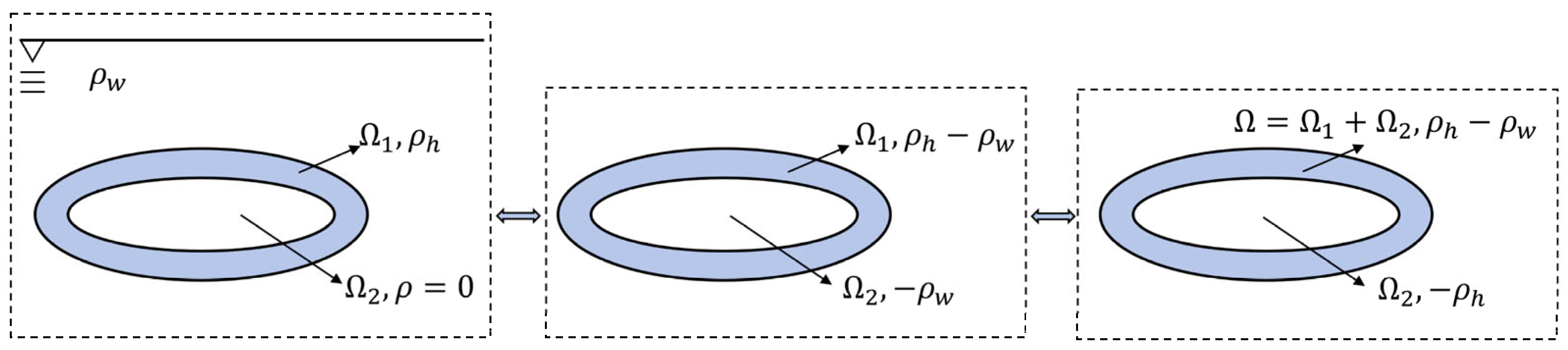
For an underwater vehicle simplified as a homogeneous rotating ellipsoid, we assume that its interior ${\mathsf{\Omega }}_2$ is hollow and that the mass is uniformly distributed on the outer hull ${\mathsf{\Omega }}_1$ with a density of ${\rho }_h$. By the superposition principle, as shown in Figure 5, the anomalous gravitational potential generated by the HEH model underwater is the superposition of the gravitational potential generated by the outer hull ${\mathsf{\Omega }}_1$ with a density of $({\rho }_h-{\rho }_w)$ and the gravitational potential generated by the inner region ${\mathsf{\Omega }}_2$ with a density of $-{\rho }_w$. The gravitational potential can be further represented as the superposition of the gravitational potential generated by an ellipsoid $\mathsf{\Omega }$ with a density of $({\rho }_h-{\rho }_w)$ and the gravitational potential generated by the inner region ${\mathsf{\Omega }}_2$ with a density of $-{\rho }_h$, i.e.,

$$\begin{gathered} V={\displaystyle \frac{4\pi Ga{b}^2\left({\rho }_h-{\rho }_w\right)}{E}}\sum _{n=0}^{\infty }{\displaystyle \frac{1}{\left(2n+1\right)\left(2n+3\right)}}{\left({\displaystyle \frac{E}{r^{\prime }}}\right)}^{2n+1}{P}_{2n}\left(\cos \alpha \right) \\ -{\displaystyle \frac{4\pi G{a}_i{b}_i^2{\rho }_h}{E_i}}\sum _{n=0}^{\infty }{\displaystyle \frac{1}{\left(2n+1\right)\left(2n+3\right)}}{\left({\displaystyle \frac{E_i}{r^{\prime }}}\right)}^{2n+1}{P}_{2n}\left(\cos \alpha \right) \\ ={\displaystyle \frac{4\pi Ga{b}^2\left({\rho }_h-{\rho }_w\right)}{E}}\sum _{n=0}^{\infty }{\displaystyle \frac{1-{\lambda }^{2n}}{\left(2n+1\right)\left(2n+3\right)}}{\left({\displaystyle \frac{E}{r^{\prime }}}\right)}^{2n+1}{P}_{2n}\left(\cos \alpha \right), \end{gathered}$$

(21)

where $a_i=\lambda a$ and $b_i=\lambda b$ are the semimajor axis and semiminor axis of the inner ellipsoid, respectively, and $E_i=\sqrt{a_i^2-b_i^2}=\lambda E$ is the linear eccentricity of the inner ellipsoid.

Next, we further investigate the gravitational field generated by the HEH. Let the coefficient

$$C={\displaystyle \frac{4\pi Ga{b}^2\left({\rho }_h-{\rho }_w\right)}{E}}.$$

(22)

In spherical coordinates $\left\{\begin{array}{c}x=r\cos \alpha \\ y=r\sin \alpha \cos \theta \\ z=r\sin \alpha \sin \theta \end{array}\right.$, the Jacobi matrix can be written as

$$J=\left[\begin{array}{ccc}{\displaystyle \frac{\partial r}{\partial x}}& {\displaystyle \frac{\partial r}{\partial y}}& {\displaystyle \frac{\partial r}{\partial z}}\\ {\displaystyle \frac{\partial \alpha }{\partial x}}& {\displaystyle \frac{\partial \alpha }{\partial y}}& {\displaystyle \frac{\partial \alpha }{\partial z}}\\ {\displaystyle \frac{\partial \theta }{\partial x}}& {\displaystyle \frac{\partial \theta }{\partial y}}& {\displaystyle \frac{\partial \theta }{\partial z}}\end{array}\right]=\left[\begin{array}{ccc}\cos \alpha & \sin \alpha \cos \theta & \sin \alpha \sin \theta \\ -{\displaystyle \frac{\sin \alpha }{r}}& {\displaystyle \frac{\cos \alpha \cos \theta }{r}}& {\displaystyle \frac{\cos \alpha \sin \theta }{r}}\\ 0& -{\displaystyle \frac{\sin \theta }{r\sin \alpha }}& {\displaystyle \frac{\cos \theta }{r\sin \alpha }}\end{array}\right].$$

(23)

The derivative of gravitational potential $V$ with respect to $x,y,z$ can be solved as

$$\begin{gathered} \left[\begin{array}{ccc}{\displaystyle \frac{\partial V}{\partial x}}& {\displaystyle \frac{\partial V}{\partial y}}& {\displaystyle \frac{\partial V}{\partial z}}\end{array}\right]=\left[\begin{array}{ccc}{\displaystyle \frac{\partial V}{\partial r}}& {\displaystyle \frac{\partial V}{\partial \alpha }}& {\displaystyle \frac{\partial V}{\partial \theta }}\end{array}\right]J \\ ={\displaystyle \frac{C}{E}}{\left[\begin{array}{c}{\displaystyle \sum _{n=0}^{\infty }}{\displaystyle \frac{{\left(\frac{E}{r^{\prime }}\right)}^{2n+2}\left(1-{\lambda }^{2n}\right)\left(2n{P}_{2n-1}\left(u\right)-\left(4n+1\right)u{P}_{2n}\left(u\right)\right)}{\left(2n+1\right)\left(2n+3\right)}}\\ -{\displaystyle \frac{\cos \theta }{\sin \alpha }}{\displaystyle \sum _{n=0}^{\infty }}{\displaystyle \frac{{\left(\frac{E}{r^{\prime }}\right)}^{2n+2}\left(1-{\lambda }^{2n}\right)\left(2nu{P}_{2n-1}\left(u\right)-\left(\left(4n+1\right)u^2-2n-1\right)P_{2n}\left(u\right)\right)}{\left(2n+1\right)\left(2n+3\right)}}\\ -{\displaystyle \frac{\sin \theta }{\sin \alpha }}{\displaystyle \sum _{n=0}^{\infty }}{\displaystyle \frac{{\left(\frac{E}{r^{\prime }}\right)}^{2n+2}\left(1-{\lambda }^{2n}\right)\left(2nu{P}_{2n-1}\left(u\right)-\left(\left(4n+1\right)u^2-2n-1\right)P_{2n}\left(u\right)\right)}{\left(2n+1\right)\left(2n+3\right)}}\end{array}\right]}^T, \end{gathered}$$

(24)

where $u=\cos \alpha$, and $\sin \alpha =\sqrt{1-u^2}$.

Furthermore, the gravity gradient generated by an HEH can be written as

$$T_{xx}={\displaystyle \frac{C}{E^2}}\sum _{n=0}^{\infty }{\displaystyle \frac{{\left(\frac{E}{r^{\prime }}\right)}^{2n+3}(1-{\lambda }^{2n})t_{xx}}{\left(2n+1\right)\left(2n+3\right)}}$$

(25)

$$T_{yy}={\displaystyle \frac{C}{E^2{\sin }^2\alpha }}\sum _{n=0}^{\infty }{\displaystyle \frac{{\left(\frac{E}{r^{\prime }}\right)}^{2n+3}(1-{\lambda }^{2n})t_{yy}}{\left(2n+1\right)\left(2n+3\right)}}$$

(26)

$$T_{xy}={\displaystyle \frac{C\cos \theta }{E^2\sin \alpha }}\sum _{n=0}^{\infty }{\displaystyle \frac{{\left(\frac{E}{r^{\prime }}\right)}^{2n+3}(1-{\lambda }^{2n})t_{xy}}{\left(2n+1\right)\left(2n+3\right)}}$$

(27)

$$T_{xz}={\displaystyle \frac{C\sin \theta }{E^2\sin \alpha }}\sum _{n=0}^{\infty }{\displaystyle \frac{{\left(\frac{E}{r^{\prime }}\right)}^{2n+3}(1-{\lambda }^{2n})t_{xz}}{\left(2n+1\right)\left(2n+3\right)}}$$

(28)

$$T_{yz}={\displaystyle \frac{C\sin \theta \cos \theta }{E^2{\sin }^2\alpha }}\sum _{n=0}^{\infty }{\displaystyle \frac{{\left(\frac{E}{r^{\prime }}\right)}^{2n+3}(1-{\lambda }^{2n})t_{yz}}{\left(2n+1\right)\left(2n+3\right)}}$$

(29)

where $t_{xx}=-2nu\left(4n+3\right)P_{2n-1}\left(u\right)+\left[\left(16n^2+16n+3\right)u^2-{\left(2n+1\right)}^2\right]P_{2n}\left(u\right)$, $t_{yy}=2nu\left[-\left(4n+3\right){\cos }^2\theta u^2+\left(4n+5\right){\cos }^2\theta -1\right]P_{2n-1}\left(u\right)+\left\{\left(16n^2+16n+3\right){\cos }^2\theta u^4-\left[20{\cos }^2\theta n^2+\left(28{\cos }^2\theta -4\right)n+6{\cos }^2\theta -1\right]u^2+\left(4n^2+8n+3\right){\cos }^2\theta -2n-1\right\}{P}_{2n}\left(u\right)$, $t_{xy}=t_{xz}=2n\left[\left(4n+3\right)u^2-2\left(n+1\right)\right]P_{2n-1}\left(u\right)+\left[-\left(16n^2+16n+3\right)u^2+12n^2+14n+3\right]u{P}_{2n}\left(u\right)$, $t_{yz}=2nu\left[4n+5-\left(4n+3\right)u^2\right]P_{2n-1}\left(u\right)+\left[\left(16n^2+16n+3\right)u^4-\left(20n^2+28n+6\right)u^2+4n^2+8n+3\right]P_{2n}\left(u\right)$.

3.3. Distribution Characteristics of the Gravitational Field a Homogeneous Ellipsoidal Hull

First, we discuss the ellipsoidal hull thickness $d$ of the HEH. We define the thickness $d$ as the radial distance between two similar ellipsoids. It is worth mentioning that $d$ is not constant. As shown in Figure 3, in our defined spherical coordinate system, the thickness $d\left(\alpha \right)$ of the ellipsoidal hull is

$$d\left(\alpha \right)=R_E-r_E={\displaystyle \frac{\left(1-\lambda \right)ab}{\sqrt{a^2{\sin }^2\alpha +b^2{\cos }^2\alpha }}}.$$

(30)

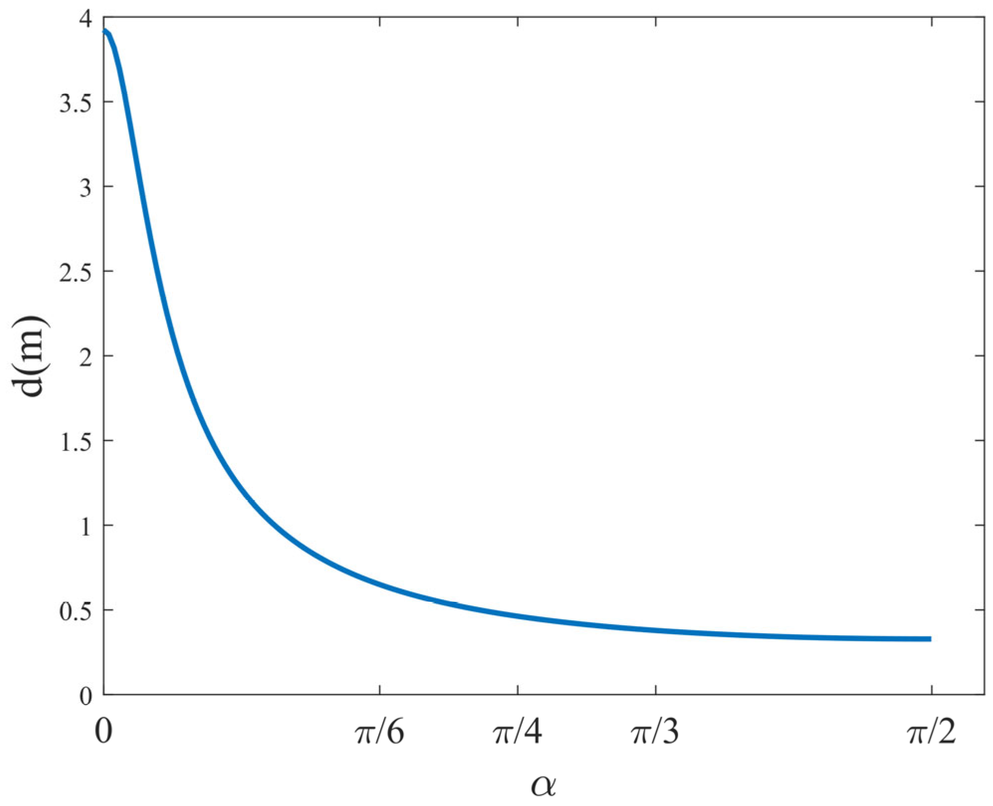
As shown in Figure 6, when $\alpha =0$ or $\pi$, the thickness of the ellipsoidal hull $d\left(\alpha \right)$ attains its maximum value $(1-\lambda )a$. When $\alpha =\pi /2$ or $3\pi /2$, the thickness of the ellipsoidal hull $d\left(\alpha \right)$ attains its minimum value $(1-\lambda )b$.

From Equations (24)–(29), the gravity anomaly and gravity gradient anomaly generated by the HEH have the following symmetry properties:

$$\left\{\begin{array}{c}f\left(x,y\right)=f\left(-x,y\right):g_y, g_z, T_{yz}, T_{xx}, T_{yy}, T_{zz}\\ f\left(x,y\right)=-f\left(-x,y\right):g_x, T_{xy}, T_{xz}\\ f\left(x,y\right)=f\left(-x,-y\right):g_x, g_z, T_{xz}, T_{xx}, T_{yy}, T_{zz}\\ f\left(x,y\right)=-f\left(-x,-y\right):g_y, T_{xy}, T_{yz}\end{array}\right..$$

(31)

Next, we study the position corresponding to the maximum absolute value of each gravity anomaly component and gravity gradient anomaly component when the sensor height $z^{\prime }$ is a fixed value $H$. From the symmetry, we only need to study the maximum absolute value of these components in the first quadrant ($x\ge 0,y\ge 0$).

We first study the maximum value of $\left|g_x\right|$ in the plane $z^{\prime }=H$. Thus, we have

$$\left\{\begin{array}{c}{T}_{xx}=0\\ T_{xy}=0\\ z^{\prime }=H\end{array}\right..$$

(32)

For the equation $T_{xy}=0$, we discard the solution $x^{\prime }=0$, because it would lead to $g_x=0$. Instead, we retain the other meaningful solution $y^{\prime }=0$, and substitute it into Equation (32) to obtain:

$$\sum _{n=0}^{\infty }{\displaystyle \frac{\left(1-{\lambda }^{2n}\right)t_{xx}}{\left(2n+1\right)\left(2n+3\right)}}{\left({\displaystyle \frac{E\sqrt{1-u^2}}{H}}\right)}^{2n+3}=0.$$

(33)

Equation (33) is a series equation in $u$, which contains an infinite number of Legendre polynomial terms and is thus difficult to solve directly for the exact solution. To simplify the calculation and obtain a practical approximate solution that meets the engineering accuracy requirements, we introduce asymptotic analysis to derive the solution. This method retains the main terms of the series (the terms with the largest contribution to the signal) and neglects the high-order small terms with negligible influence. This approach not only simplifies the solving process but also ensures the physical validity of the solution. Equation (33) can be rewritten as

$$\sum _{n=0}^{\infty }{A}_n\left(u\right){\delta }^{2n+3}=0$$

(34)

where $A_n(u)={\displaystyle \frac{\left(1-{\lambda }^{2n}\right)\left\{-2nu\left(4n+3\right)P_{2n-1}\left(u\right)+\left[\left(16n^2+16n+3\right)u^2-{\left(2n+1\right)}^2\right]P_{2n}\left(u\right)\right\}}{\left(2n+1\right)\left(2n+3\right)}}{\left(\sqrt{1-u^2}\right)}^{2n+3}$, and $\delta =E/H$. Since Legendre polynomials have parity, that is, $P_{2n-1}\left(-u\right)=-P_{2n-1}\left(u\right)$ and $P_{2n}\left(-u\right)=P_{2n}\left(u\right)$, it can be found that $A_n\left(-u\right)=A_n\left(u\right)$. In addition, assuming that $u\left(\delta \right)$ is the solution of Equation (34), if $\delta$ is replaced with $-\delta$ in Equation (34), we have

$$\sum _{n=0}^{\infty }{A}_n\left(u\right(-\delta \left)\right){(-\delta )}^{2n+3}=-\sum _{n=0}^{\infty }{A}_n\left(u\left(-\delta \right)\right){\delta }^{2n+3}=0.$$

(35)

From Equation (35), it follows that if $u\left(\delta \right)$ is a solution of Equation (34), then $u(-\delta )$ is also a solution of Equation (34). Therefore, the solution of Equation (34) can be written as

$$u=\sum _{n=0}^{\infty }{u}_{2n}{\delta }^{2n}$$

(36)

with unknown coefficients $u_{2n}$. Perform the Taylor expansion of $A_n\left(u\right)$ at $u_0$:

$$A_n\left(u\right)=A_n\left(u_0\right)+A_n^{\prime }\left(u_0\right)\left(u-u_0\right)+{\displaystyle \frac{1}{2!}}{A}_n^{″}\left(u_0\right){\left(u-u_0\right)}^2+o\left({\left(u-u_0\right)}^2\right).$$

(37)

Substitute Equations (36) and (37) into Equation (34), and collect the terms according to the powers of $\delta$ to obtain:

$${\delta }^5\left(n=1\right):A_1\left(u_0\right)=0⟹35u_0^4-30u_0^2+3=0⟹u_0=\sqrt{{\displaystyle \frac{15-2\sqrt{30}}{35}}}$$

(38)

$${\delta }^7\left(n=1,2\right):A_1^{\prime }\left(u_0\right)u_2+A_2\left(u_0\right)=0⟹u_2=-{\displaystyle \frac{A_2\left(u_0\right)}{A_1^{\prime }\left(u_0\right)}}$$

(39)

$$\begin{gathered} {\delta }^9\left(n=1,2,3\right):\&A_1^{\prime }\left(u_0\right)u_4+{\displaystyle \frac{1}{2}}{A}_1^{″}\left(u_0\right)u_2^2+A_2^{\prime }\left(u_0\right)u_2+A_3\left(u_0\right)=0 \\ ⟹u_4=-{\displaystyle \frac{\frac{1}{2}{A}_1^{″}\left(u_0\right)u_2^2+A_2^{\prime }\left(u_0\right)u_2+A_3\left(u_0\right)}{A_1^{\prime }\left(u_0\right)}}. \end{gathered}$$

(40)

Since Equation (36) converges rapidly as $n$ increases, we only need to calculate up to $n=2$.

Similarly, to find the maximum value of $\left|T_{xz}\right|$ on the plane $z^{\prime }=H$, we retain the solution $y^{\prime }=0$ and substitute it into $T_{xxz}=0$ to obtain:

$$\sum _{n=0}^{\infty }{\displaystyle \frac{\left(1-{\lambda }^{2n}\right)t_{xxz}}{\left(2n+1\right)\left(2n+3\right)}}{\left({\displaystyle \frac{E\sqrt{1-u^2}}{H}}\right)}^{2n+4}=0$$

(41)

where $t_{xxz}=2nu\left[-\left(4n+3\right)(4n+5)u^2+12n^2+26n+13\right]P_{2n-1}\left(u\right)+\left[\left(4n+1\right)\left(4n+3\right)\left(4n+5\right)u^4-2\left(4n+3\right)\left(8n^2+13n+3\right)u^2+{\left(2n+1\right)}^2\left(2n+3\right)\right]P_{2n}\left(u\right)$. Equation (41) has a solution in the same form as Equation (36), with the only modification being the replacement of $A_n\left(u\right)$ by

$$A_n\left(u\right)={\displaystyle \frac{\left(1-{\lambda }^{2n}\right){\left(\sqrt{1-u^2}\right)}^{2n+4}{t}_{xxz}}{\left(2n+1\right)\left(2n+3\right)}},$$

(42)

and replacing $u_0$ with $u_0=\sqrt{{\displaystyle \frac{7-2\sqrt{7}}{21}}}$.

Conversely, to find the maximum value of $\left|g_y\right|$ on the plane $z^{\prime }=H$, we retain the solution $x^{\prime }=0$ and substitute it into $T_{yy}=0$ to obtain:

$$\sum _{n=0}^{\infty }{\left({\displaystyle \frac{Ev}{H}}\right)}^{2n+3}\left(1-{\lambda }^{2n}\right)\left(1-v^2-{\displaystyle \frac{1}{2n+3}}\right)P_{2n}\left(0\right)=0,$$

(43)

where $v=\sin \theta$. Equation (43) has a solution form similar to Equation (36):

$$v=\sum _{n=0}^{\infty }{v}_{2n}{\delta }^{2n},$$

(44)

where

$$\left\{\begin{array}{c}{A}_n\left(v\right)=\left(1-{\lambda }^{2n}\right)\left(1-v^2-{\displaystyle \frac{1}{2n+3}}\right)P_{2n}\left(0\right)v^{2n+3}\\ v_0={\displaystyle \frac{2\sqrt{5}}{5}}\\ v_2=-{\displaystyle \frac{A_2\left(v_0\right)}{A_1^{\prime }\left(v_0\right)}}\\ v_4=-{\displaystyle \frac{\frac{1}{2}{A}_1^{″}\left(v_0\right)v_2^2+A_2^{\prime }\left(v_0\right)v_2+A_3\left(v_0\right)}{A_1^{\prime }\left(v_0\right)}}\end{array}\right..$$

(45)

To find the maximum value of $\left|T_{yz}\right|$ on the plane $z^{\prime }=H$, we retain the solution $x^{\prime }=0$ and substitute it into $T_{yyz}=0$ to obtain:

$$\sum _{n=0}^{\infty }{\left({\displaystyle \frac{Ev}{H}}\right)}^{2n+4}\left(1-{\lambda }^{2n}\right) \left[\left(2n+5\right)\right(1-v^2)-1]P_{2n}\left(0\right)=0.$$

(46)

Equation (46) has a solution in the same form as Equations (44) and (45), with the only modification being the replacement of $A_n\left(v\right)$ by

$$A_n\left(v\right)=\left(1-{\lambda }^{2n}\right)\left(\left(2n+5\right)(1-v^2)-1\right)P_{2n}\left(0\right)v^{2n+4},$$

(47)

and replacing $v_0$ with $v_0=\sqrt{6/7}$.

To find the maximum value of $\left|T_{xy}\right|$ on the plane $z^{\prime }=H$, we have

$$\left\{\begin{array}{c}{\displaystyle \sum _{n=0}^{\infty }}{\displaystyle \frac{{\left(\frac{E}{r^{\prime }}\right)}^{2n+4}\left(1-{\lambda }^{2n}\right)t_{xxy}}{\left(2n+1\right)\left(2n+3\right)}}=0\\ {\displaystyle \sum _{n=0}^{\infty }}{\displaystyle \frac{{\left(\frac{E}{r^{\prime }}\right)}^{2n+4}\left(1-{\lambda }^{2n}\right)t_{xyy}}{\left(2n+1\right)\left(2n+3\right)}}=0\\ z^{\prime }=H\end{array}\right.$$

(48)

where $t_{xxy}=\left[\left(4n+1\right)\left(4n+3\right)\left(4n+5\right)u^4-2\left(4n+3\right)\left(6n^2+13n+3\right)u^2+{\left(2n+1\right)}^2\left(2n+3\right)\right]P_{2n}\left(u\right)+2nu\left[-4\left(2n+1\right)\left(4n+3\right)u^2+12n^2+26n+13\right]P_{2n-1}\left(u\right)$, $t_{xyy}=\left\{\left(4n+1\right)\left(4n+3\right)\left(4n+5\right){\cos }^2\theta u^4-\left(4n+3\right)\left[2{\cos }^2\theta \left(12n^2+22n+5\right)-4n-1\right]u^2+{\cos }^2\theta \left(32n^3+96n^2+76n+15\right)-12n^2-14n-3\right\}u{P}_{2n}\left(u\right)-2n\left\{\left(4n+3\right)\left(4n+5\right){\cos }^2\theta u^4-\left[(20n^2+48n+25){\cos }^2\theta -4n-3\right]u^2+2\left(n+1\right)\left[\left(2n+4\right){\cos }^2\theta -1\right]\right\}{P}_{2n-1}\left(u\right)$.

Equation (48) can be rewritten as

$$\left\{\begin{array}{c}{\displaystyle \sum _{n=0}^{\infty }}{A}_n{\delta }^n=0\\ {\displaystyle \sum _{n=0}^{\infty }}{B}_n{\delta }^n=0\\ z^{\prime }=H\end{array}\right.$$

(49)

where $A_n(u,v)={\displaystyle \frac{\left(1-{\lambda }^{2n}\right)t_{xxy}}{\left(2n+1\right)\left(2n+3\right)}}{\left(\sqrt{1-u^2}v\right)}^{2n+4}$, $B_n(u,v)={\displaystyle \frac{\left(1-{\lambda }^{2n}\right)t_{xyy}}{\left(2n+1\right)\left(2n+3\right)}}{\left(\sqrt{1-u^2}v\right)}^{2n+4}$. It can be seen that, in this case, $A_n(u,v)$ contains both variables $u$ and $v$, which are separable, whereas the variables $u$ and $v$ in $B_n(u,v)$ are inseparable. Similarly, we assume that

$$\left\{\begin{array}{c}u=u_0+u_2{\delta }^2+u_4{\delta }^2+O\left({\delta }^6\right)\\ v=v_0+v_2{\delta }^2+v_4{\delta }^4+O\left({\delta }^6\right)\end{array}\right..$$

(50)

Perform a Taylor expansion of $A_n(u,v)$ and $B_n(u,v)$ at the point $(u_0,v_0)$:

$$\begin{gathered} f_n\left(u,v\right)=f_n\left(u_0,v_0\right)+{\displaystyle \frac{\partial f_n\left(u_0,v_0\right)}{\partial u}}\left(u_2{\delta }^2+u_4{\delta }^2\right)+{\displaystyle \frac{\partial f_n\left(u_0,v_0\right)}{\partial v}}\left(v_2{\delta }^2+v_4{\delta }^2\right) \\ +{\displaystyle \frac{1}{2}}{\displaystyle \frac{\partial f_n^2\left(u_0,v_0\right)}{\partial u^2}}{u}_2^2{\delta }^4+{\displaystyle \frac{\partial f_n^2\left(u_0,v_0\right)}{\partial u\partial v}}{u}_2{v}_2{\delta }^4+{\displaystyle \frac{1}{2}}{\displaystyle \frac{\partial f_n^2\left(u_0,v_0\right)}{\partial v^2}}{v}_2^2{\delta }^4+O({\delta }^6) \end{gathered}$$

(51)

where $f_n=A_n$ or $B_n$.

Similarly, we collect the terms according to the powers of $\delta$. Considering the term of order ${\delta }^6\left(n=1\right)$, we have

$$A_1\left(u_0,v_0\right)=-{\displaystyle \frac{9}{2}}{\left(1-u_0^2\right)}^4{v}_0^6(21u_0^4-14u_0^2+1)=0⟹u_0=\sqrt{{\displaystyle \frac{7-2\sqrt{7}}{21}}}$$

(52)

$$\begin{gathered} B_1\left(u_0,v_0\right)={\displaystyle \frac{u_0}{2}}{\left(1-u_0^2\right)}^4{v}_0^6\left[21\left(3u_0^4-4u_0^2+1\right)v_0^2-\left(63u_0^4-77u_0^2+18\right)\right]=0 \\ ⟹v_0=\sqrt{{\displaystyle \frac{63u_0^4-77u_0^2+18}{21\left(3u_0^4-4u_0^2+1\right)}}}=\sqrt{{\displaystyle \frac{5}{6}}}. \end{gathered}$$

(53)

Considering the term of order ${\delta }^8\left(n=1,2\right)$, we have

$${\displaystyle \frac{\partial f_1\left(u_0,v_0\right)}{\partial u}}{u}_2+{\displaystyle \frac{\partial f_1\left(u_0,v_0\right)}{\partial v}}{v}_2+f_2\left(u_0,v_0\right)=0$$

(54)

where ${\displaystyle \frac{\partial A_1\left(u_0,v_0\right)}{\partial v}}=0$. Therefore,

$$u_2=-{\displaystyle \frac{A_2\left(u_0,v_0\right)}{\frac{\partial A_1\left(u_0,v_0\right)}{\partial u}}},v_2=-{\displaystyle \frac{\frac{\partial B_1\left(u_0,v_0\right)}{\partial u}{u}_2+B_2\left(u_0,v_0\right)}{\frac{\partial B_1\left(u_0,v_0\right)}{\partial v}}}.$$

(55)

Considering the term of order ${\delta }^{10}\left(n=1,2,3\right)$, we have

$$\begin{gathered} {\displaystyle \frac{\partial f_1\left(u_0,v_0\right)}{\partial u}}{u}_4+{\displaystyle \frac{\partial f_1\left(u_0,v_0\right)}{\partial v}}{v}_4+{\displaystyle \frac{1}{2}}{\displaystyle \frac{\partial f_1^2\left(u_0,v_0\right)}{\partial u^2}}{u}_2^2+{\displaystyle \frac{\partial f_1^2\left(u_0,v_0\right)}{\partial u\partial v}}{u}_2{v}_2+{\displaystyle \frac{1}{2}}{\displaystyle \frac{\partial f_1^2\left(u_0,v_0\right)}{\partial v^2}}{v}_2^2 \\ +{\displaystyle \frac{\partial f_2\left(u_0,v_0\right)}{\partial u}}{u}_2+{\displaystyle \frac{\partial f_2\left(u_0,v_0\right)}{\partial v}}{v}_2+f_3\left(u_0,v_0\right)=0. \end{gathered}$$

(56)

Substituting ${\displaystyle \frac{\partial A_1\left(u_0,v_0\right)}{\partial v}}=0$ into Equation (56), we obtain

$$u_4=-{\displaystyle \frac{\partial A_1\left(u_0,v_0\right)}{\partial u}}·\left(\begin{array}{c}{\displaystyle \frac{1}{2}}{\displaystyle \frac{\partial A_1^2\left(u_0,v_0\right)}{\partial u^2}}{u}_2^2+{\displaystyle \frac{\partial A_1^2\left(u_0,v_0\right)}{\partial u\partial v}}{u}_2{v}_2+{\displaystyle \frac{1}{2}}{\displaystyle \frac{\partial A_1^2\left(u_0,v_0\right)}{\partial v^2}}{v}_2^2\\ +{\displaystyle \frac{\partial A_2\left(u_0,v_0\right)}{\partial u}}{u}_2+{\displaystyle \frac{\partial A_2\left(u_0,v_0\right)}{\partial v}}{v}_2+A_3\left(u_0,v_0\right)\end{array}\right).$$

(57)

Substituting Equation (57) into Equation (56), we obtain

$$v_4=-{\displaystyle \frac{\partial B_1\left(u_0,v_0\right)}{\partial u}}·\left(\begin{array}{c}{\displaystyle \frac{\partial B_1\left(u_0,v_0\right)}{\partial u}}{u}_4+{\displaystyle \frac{1}{2}}{\displaystyle \frac{\partial B_1^2\left(u_0,v_0\right)}{\partial u^2}}{u}_2^2+{\displaystyle \frac{\partial B_1^2\left(u_0,v_0\right)}{\partial u\partial v}}{u}_2{v}_2+{\displaystyle \frac{1}{2}}{\displaystyle \frac{\partial B_1^2\left(u_0,v_0\right)}{\partial v^2}}{v}_2^2\\ +{\displaystyle \frac{\partial B_2\left(u_0,v_0\right)}{\partial u}}{u}_2+{\displaystyle \frac{\partial B_2\left(u_0,v_0\right)}{\partial v}}{v}_2+B_3\left(u_0,v_0\right)\end{array}\right).$$

(58)

The absolute maximum values of the remaining gravity anomaly components and gravity gradient anomaly components $(g_z,T_{xx},T_{yy},T_{zz})$ on the plane $z^{\prime }=H$ are all attained at the point $(0, 0)$.

4. Case Analysis

In this section, we apply the HEH model to several typical underwater vehicles, as listed in

Table 1. Parameters of several typical underwater vehicles.

Target	a (m)	${\mathit{m}}_{\downarrow }$ (kg)	E (m)	$\mathit{\lambda }$
HEH-M1 (18,750 t)	85.35	1.875 $\times {10}^7$	85.05	0.9540
HEH-M2 (6927 t)	55.15	6.927 $\times {10}^6$	54.89	0.9540
HEH-M3 (1320 t)	37.35	1.320 $\times {10}^6$	37.24	0.9540
HEH-M1-$\mathsf{\lambda }$1 (18,750 t)	85.35	1.875 $\times {10}^7$	85.05	0.9156
HEH-M1-$\mathsf{\lambda }$2 (18,750 t)	85.35	1.875 $\times {10}^7$	85.05	0.8520

, to analyze the gravity anomaly and gravity gradient anomaly generated by them. For HEH-M1-$\mathsf{\lambda }$1 and HEH-M1-$\mathsf{\lambda }$2, the displacement and geometry are identical to those of HEH-M1, while the similarity ratio $\mathsf{\lambda }$ is varied to represent different hull material densities.

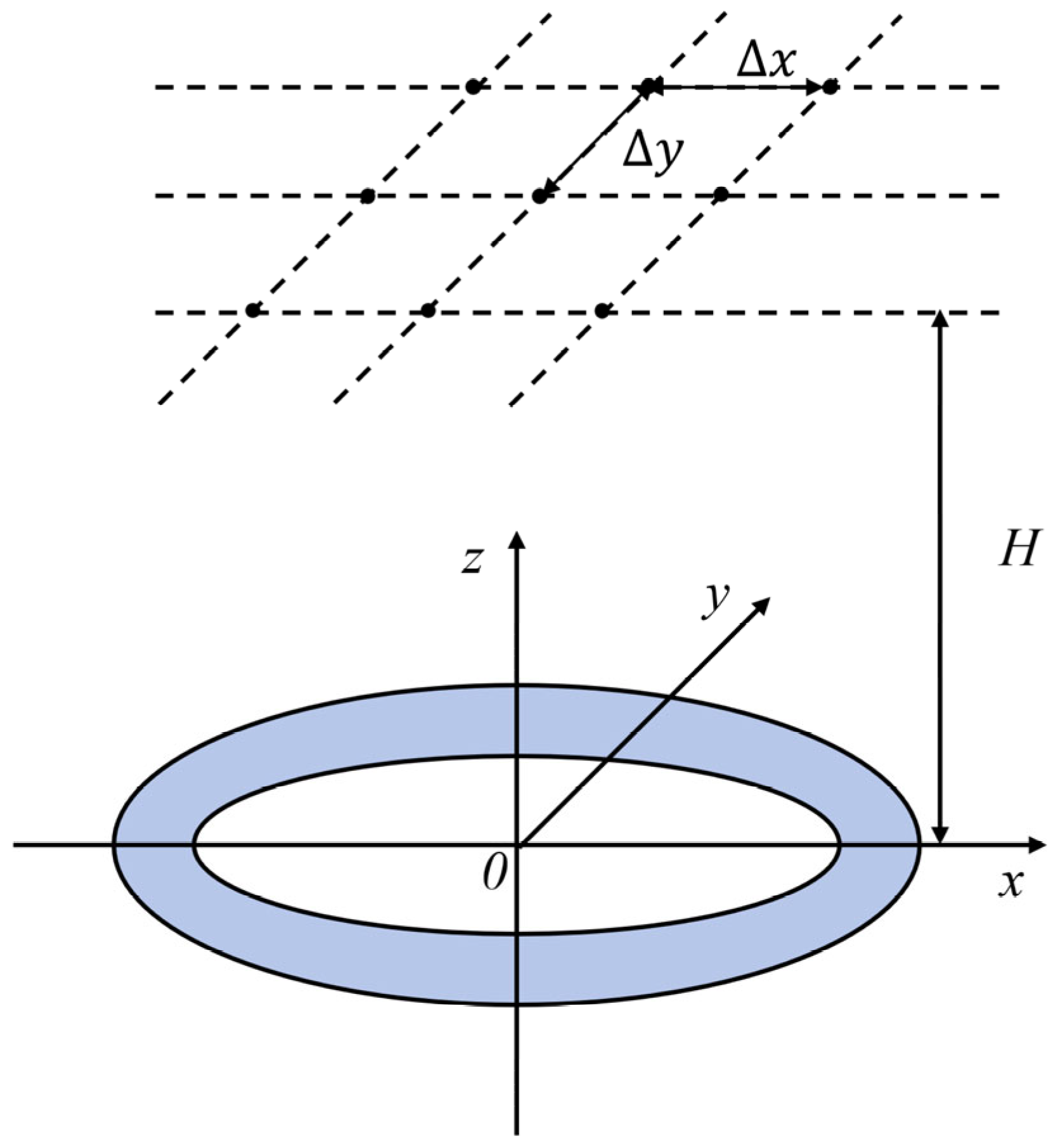
The proposed model and method were validated on MATLAB R2023b. We established a measurement grid consisting of 101 $\times$ 101 points, with a uniform grid spacing of $∆x=∆y=$ 20 m, covering an area of 2 km $\times$ 2 km, as illustrated in Figure 7. The height of the measurement grid was sequentially set to 100, 120, 140, 160, 180, 200, 250, 300, and 400 m to investigate the magnitudes of the gravity anomaly components and gravity gradient components at different measurement heights.

4.1. Gravitational Field and GGT Generated by HEH

First, taking the HEH-M1 (18,750 t) as an example, it has a submerged displacement of 18,750 t, a length of 170.7 m, and a width of 12.8 m. When modeled as an HEH, its semi-major axis is $a=$ 85.35 m. Given the seawater density ${\rho }_w=1.03\times {10}^3 \mathrm{k}\mathrm{g}/{\mathrm{m}}^3$, the semi-minor axis is calculated as $b=\sqrt{3m_{\downarrow }/\left(4\pi a{\rho }_w\right)}=$ 7.14 m. Assume that the hull is made of high-strength steel with a density of ${\rho }_h=7.82\times {10}^3 \mathrm{k}\mathrm{g}/{\mathrm{m}}^3$.

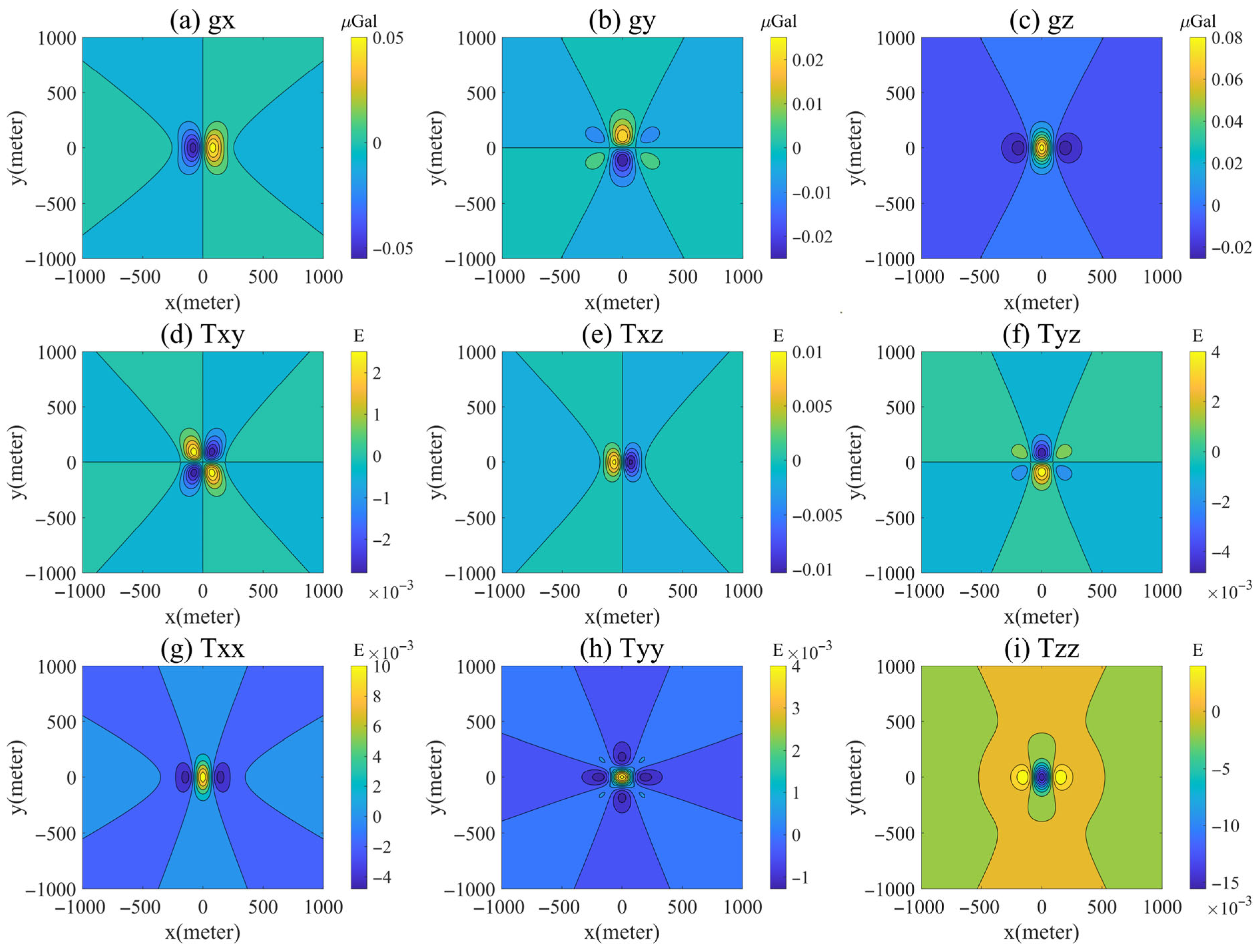
Figure 8 displays the three gravity anomaly components and six gravity gradient anomaly components generated by HEH-M1 on the plane $z=200$ m. These components exhibit the symmetries mentioned in Section 3. Moreover, even within the first quadrant, these components are not uniformly positive or negative. For the three gravity anomaly components $(g_x,g_y,g_z)$ and the three off-diagonal gravity gradient anomaly components ($T_{xy},T_{xz},T_{yz}$), only one curve separates the regions of positive and negative values. However, for the three diagonal gravity gradient components ($T_{xx},T_{yy},T_{zz}$), two curves delineate the regions of positive and negative values. Furthermore, among the absolute maximum values of these six gravity gradient components, $T_{zz}$ has the largest absolute value. On one hand, since $T_{xx}$ and $T_{yy}$ have the same sign and $T_{xx}+T_{yy}+T_{zz}=0$, $T_{zz}$ naturally has the largest absolute value among the three diagonal components. On the other hand, comparing the maximum values of $T_{zz}$ and the three off-diagonal gravity gradient components (taking $T_{yz}$ as an example) on the plane $z=H(H>E)$, the respective maximum values are

$$T_{zz}\left(0,0,H\right)={\displaystyle \frac{C}{E^2}}\sum _{n=0}^{\infty }{\displaystyle \frac{{\left(\frac{E}{H}\right)}^{2n+3}\left(1-{\lambda }^{2n}\right)\left(2n+2\right)P_{2n}\left(0\right)}{2n+3}}$$

(59)

$$T_{yz}\left(0,y,H\right)={\displaystyle \frac{C\sin \theta \cos \theta }{E^2}}\sum _{n=0}^{\infty }{\left({\displaystyle \frac{Ev}{H}}\right)}^{2n+3}\left(1-{\lambda }^{2n}\right)P_{2n}\left(0\right).$$

(60)

By comparing Equations (59) and (60), it can be observed that $T_{yz}(0,y,H)$ incorporates additional factors of $v^{2n+3}$ and $\sin \theta \cos \theta$, both of which are less than 1. Moreover, $v^{2n+3}$ rapidly decays as $n$ increases. In contrast, although the extra factor $\left(2n+2\right)/(2n+3)$ in $T_{zz}\left(0,0,H\right)$ is also less than 1, it is closer to 1. Therefore, on the plane $z=H(H>E)$, among the absolute maximum values of the six gravity gradient components, $T_{zz}$ has the largest absolute value.

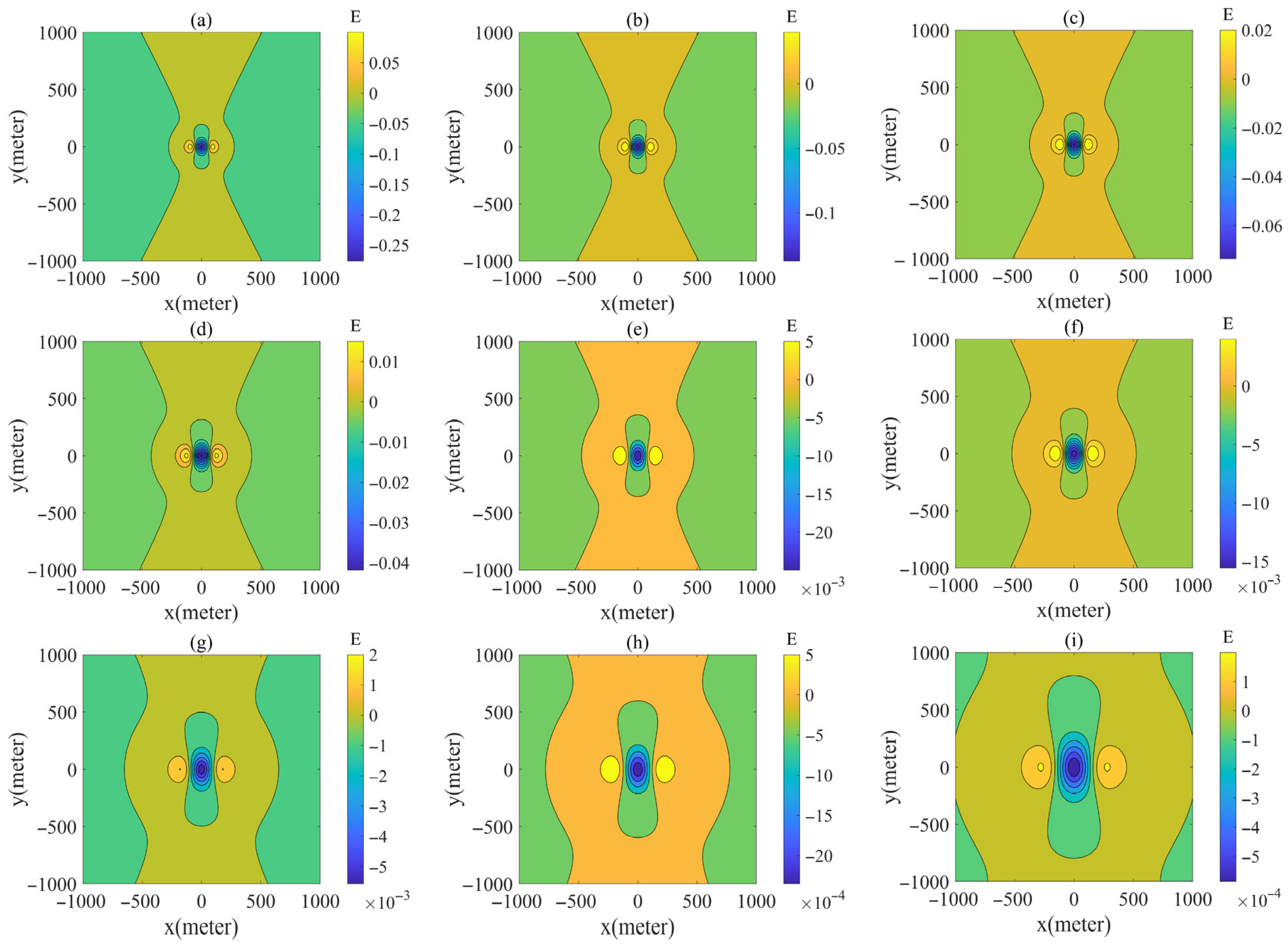
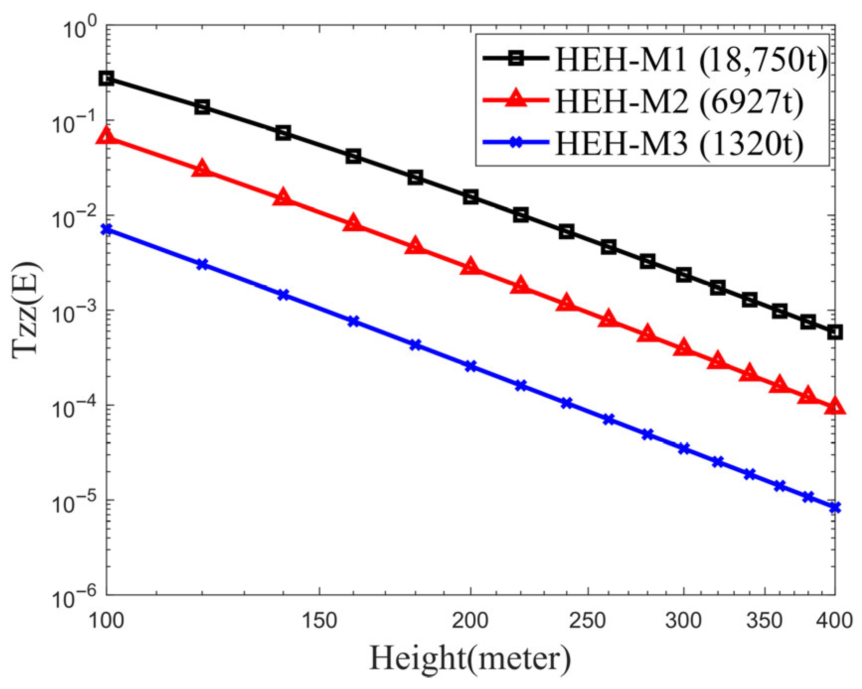
Next, we further investigate the distribution of the $T_{zz}$ component on the planes $z=H$ ($H$ varies). As illustrated in Figure 9, $T_{zz}$ is divided by zero-value lines into three regions with alternating positive and negative values: (i) the main signal region, located directly above the HEH, where $T_{zz}$ is negative; (ii) the inner sidelobe regions, flanking the main signal region, where $T_{zz}$ is positive; and (iii) the outer sidelobe regions, situated outside the inner sidelobe regions, where $T_{zz}$ is negative. As $H$ increases, the zero-value lines extend outward, meaning that both the main signal region and the inner sidelobe regions expand outward. Simultaneously, the absolute value of $T_{zz}$ rapidly decays with increasing $H$. To further characterize this decay trend, Figure 10 displays the variation of $T_{zz}\left(0,0,H\right)$ with $H$ for Targets 1 to 3, which differ in length and displacement but share the same material properties (i.e., the same $\lambda$). As shown in Figure 10, $T_{zz}$ decays rapidly with increasing $H$, roughly following a power-law function. This is because, in Equation (58), the series converges rapidly as $n$ increases. If only the first two non-zero terms $(n=1,2)$ are considered, $T_{zz}(0,0,H)$ is approximately inversely proportional to $H^k$, where $k\in (4,5)$ is related to $E$.

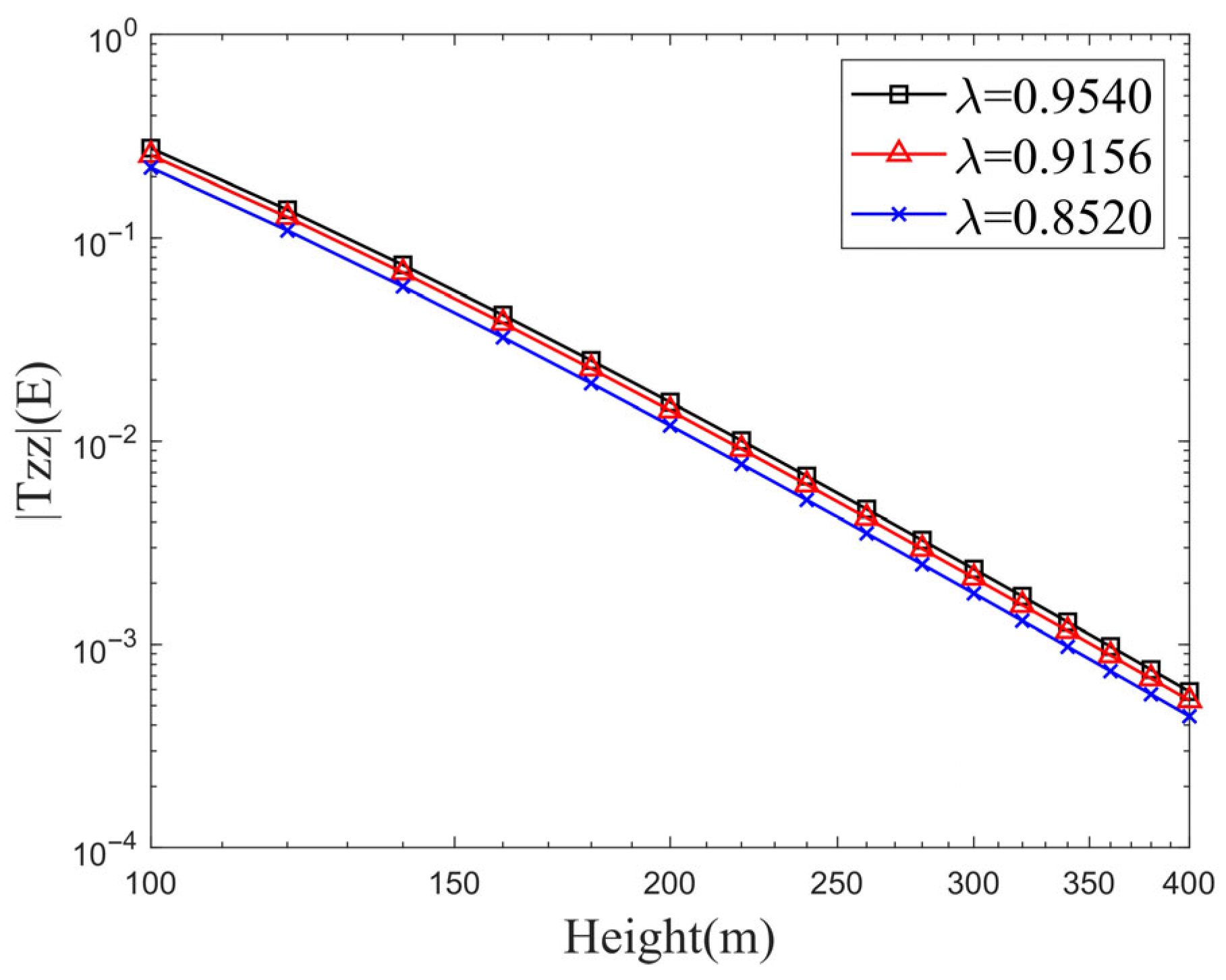
We further investigated the influence of the parameter $\lambda$ on $T_{zz}$. The parameter $\lambda$ depends solely on the seawater density ${\rho }_w$ and the hull material density ${\rho }_s$, as described in Equation (3). Typically, the variation in seawater density is relatively small; here, we take ${\rho }_w=$1030 $\mathrm{k}\mathrm{g}/{\mathrm{m}}^3$, while ${\rho }_h$ is set to 7820, 4430, and 2700 $\mathrm{k}\mathrm{g}/{\mathrm{m}}^3$, corresponding to the densities of high-density materials (e.g., high-strength steel), medium-density materials (e.g., titanium alloy), and low-density materials (e.g., aluminum alloy), respectively. Consequently, $\lambda$ takes values of 0.9540, 0.9156, and 0.8520, respectively. There are two instances in Equation (58) where the parameter $\lambda$ is involved: $C=4\pi Ga{b}^2{\rho }_w\left({\displaystyle \frac{1}{1-{\lambda }^3}}-1\right)/E$ and the coefficient $\left(1-{\lambda }^{2n}\right)$ in the series. Given that the series in Equation (58) converges rapidly as $n$ increases, we only consider the coefficient related to $\lambda$ in the first non-zero term (i.e., when $n=1$), which is ${\lambda }^3(1+\lambda )/(1+\lambda +{\lambda }^2)$. Therefore, as $\lambda$ increases, the coefficient related to $\lambda$ in Equation (58) increases slowly, and $\left|T_{zz}\right|$ also increases correspondingly at a slow rate. The $\left|T_{zz}\right|$ values corresponding to the three sets of $\lambda$ values listed in Table 1 at the same position $(0,0,H)$ are still within the same order of magnitude, as shown in Figure 11.

4.2. Feasibility Analysis of Using $T_{zz}$ for Underwater Vehicle Detection

We have theoretically investigated the absolute maximum values of the six gravity gradient anomaly components on the plane $z=H\left(H>E\right)$ and arrived at the conclusion that directly above the target, $T_{zz}$ is typically the gravity gradient component with the largest absolute value. This implies that in the most critical detection area, $T_{zz}$ provides the strongest signal, not only in terms of the largest signal amplitude but also with the broadest main signal region, as illustrated in Figure 8. $T_{zz}$ exhibits a “negative-positive-negative” distribution pattern above the target, with its absolute maximum value occurring at $(0,0,H)$, which enhances data interpretability. In contrast, other off-diagonal components have zero values along certain axes directly above the target; for example, $T_{xz}$ is zero along the $x=0$ axis, while its maximum value on the plane $z=H$ is located at $(x_0,0,H)$. This increases the complexity of data interpretation since the maximum anomaly does not appear directly above the target. Furthermore, on the Earth’s surface, the vertical variation in the normal background gravitational field is the most stable. Although the background noise is significant, it represents a globally consistent, smooth, and precisely modellable, predictable, and compensable quantity. In local detection, we can subtract this background model from the observed values, leaving the anomalous field as the target signal. In contrast, the background fields of the horizontal components $(T_{xy},T_{yy},T_{xy})$ are more complex and susceptible to influences from terrain and regional geological structures, making them difficult to accurately isolate and resulting in a lower signal-to-noise ratio. In summary, $T_{zz}$ is the optimal component to serve as the detection signal source among the above nine components.

Currently, internationally advanced marine and airborne gravity gradiometer systems have achieved an accuracy level ranging from 5 E@ 100 s integration to 60 E/√Hz, while laboratory-level gravity gradiometers have reached resolutions around ${10}^{-4}$ E under optimized conditions. With the continued development of superconducting technology, the sensitivity of gravity gradiometers is expected to improve, potentially reaching ${10}^{-6}$ E in the future [31]. The vertical gravity gradient $T_{zz}$ generated by the first three models in Table 1 can be calculated using Equation (59), and the calculation results are shown in

Table 2. Accuracy requirements for gravity gradient detection platforms at different altitudes.

Height (m)	100	300	500	1000	1500
$T_{zz}$ of HEH-M1 (E)	2.76$\times {10}^{-1}$	2.35$\times {10}^{-3}$	1.97$\times {10}^{-4}$	6.36$\times {10}^{-6}$	8.43$\times {10}^{-7}$
$T_{zz}$ of HEH-M2 (E)	6.59$\times {10}^{-2}$	3.87$\times {10}^{-4}$	3.11$\times {10}^{-5}$	9.85$\times {10}^{-7}$	1.30$\times {10}^{-7}$
$T_{zz}$ of HEH-M3 (E)	7.11$\times {10}^{-3}$	3.49$\times {10}^{-5}$	2.75$\times {10}^{-6}$	8.66$\times {10}^{-8}$	1.14$\times {10}^{-8}$

. If the accuracy of the gravity gradiometer reaches ${10}^{-2}$ E, the detectable height for HEH-M1 can reach approximately 220 m, around 150 m for HEH-M2, and about 90 m for HEH-M3. If the accuracy improves to ${10}^{-4}$ E, the detectable height increases to roughly 570 m for HEH-M1, approximately 390 m for HEH-M2, and about 240 m for HEH-M3. If the accuracy further reaches ${10}^{-6}$ E, the detectable height extends to around 1450 m for HEH-M1, approximately 1000 m for HEH-M2, and about 610 m for HEH-M3. Therefore, the use of a gravity gradiometer for underwater vehicle detection holds promising development prospects, which calls for further research into relevant theories and methods.

4.3. Comparison with Other Models

Since $T_{zz}$ provides better feasibility for underwater vehicle detection, we only compare the vertical gradient component $T_{zz}$ generated by the proposed HEH model with those generated by the HEM, TSM, and GDM.

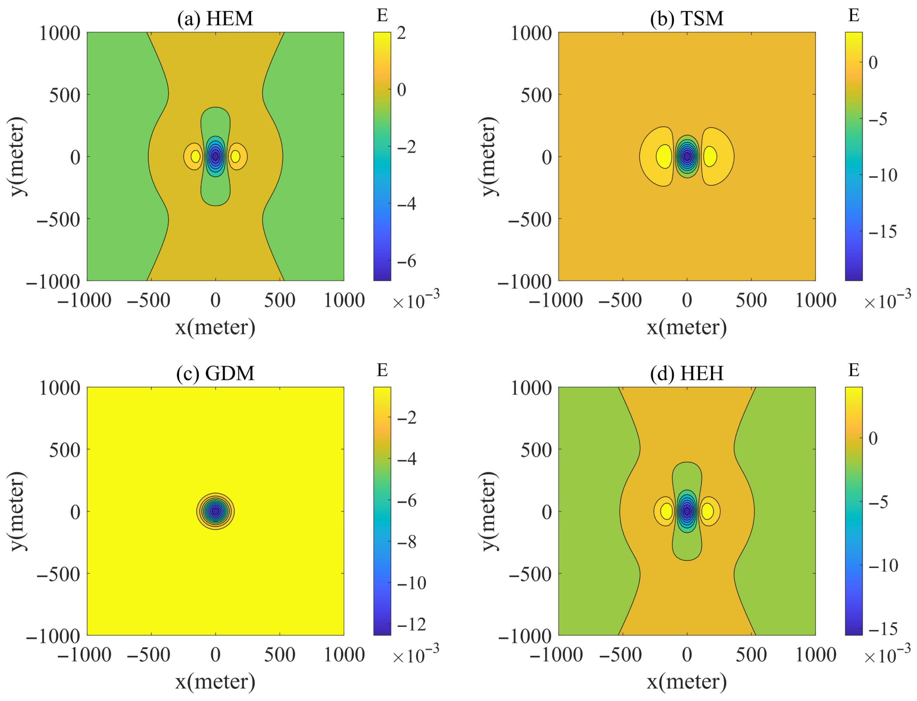
Figure 12 shows the $T_{zz}$ distribution calculated by the above four models for the same target HEH-M1 (18,750 t) on the plane at $z=$ 200 m. The HEH model exhibits an almost identical distribution to the HEM, differing only in magnitude, because the two models share the same geometric assumptions, with the only distinction being that the HEH model accounts for the shell thickness. The vertical gravity gradient $T_{zz}$ generated by the TSM is characterized by negative values in the center and positive values at the periphery, with a slightly larger amplitude than that generated by the HEH model. This arises because the TSM incorporates the feature that the center of gravity of the underwater vehicle lies below the center of buoyancy, leading to an additional contribution from the uneven vertical mass distribution. Although the GDM also accounts for the uneven vertical mass distribution of the underwater vehicle, it greatly simplifies its structural characteristics: the upper half is approximated as a negative point mass and the lower half as a positive point mass. This superposition results in a vertical gravity gradient field that is negative in the center and positive at the periphery, with circular contour lines.

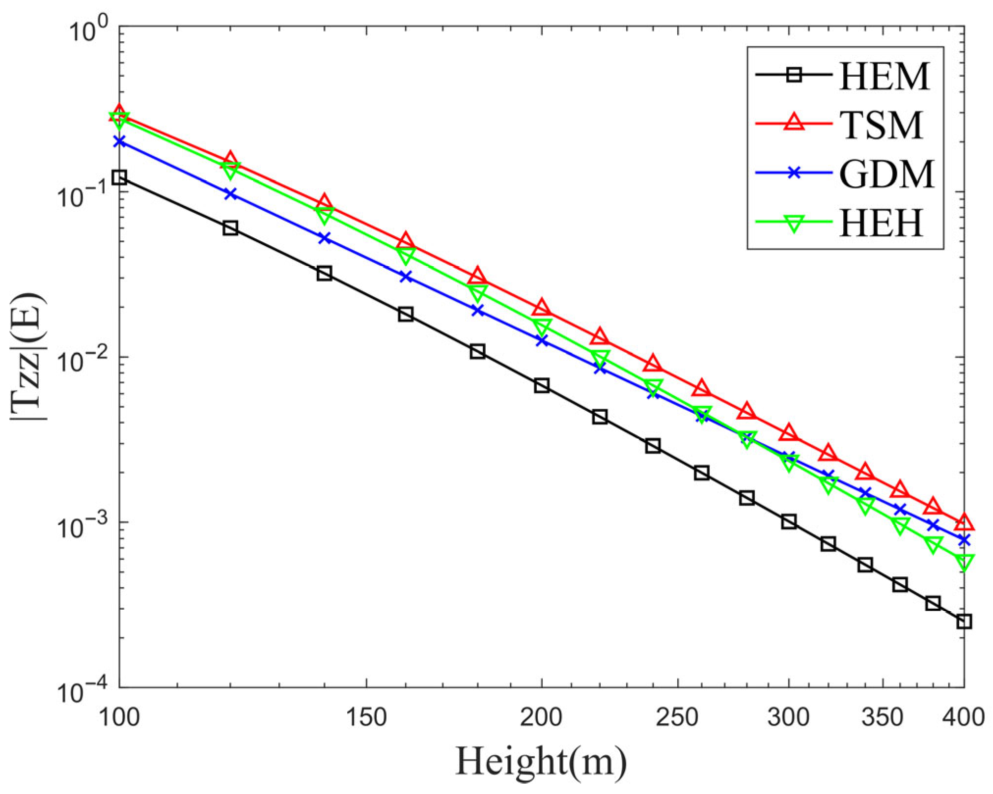
Figure 13 presents the variation of $T_{zz}(0,0,H)$ with $H$ calculated using the four models. For 100 m $<H<$ 270 m, the $T_{zz}$ values at the same altitude rank in descending order as follows: TSM, HEH, GDM, HEM. For 270 m $<H<$ 400 m, the order becomes TSM, GDM, HEH, HEM. The TSM accounts for the vertical mass difference and yields the largest $T_{zz}$. Although the GDM also considers vertical mass asymmetry, it drastically simplifies the vehicle geometry, resulting in significantly smaller $T_{zz}$ than that of the TSM in the near field. As $H$ increases, the difference between them gradually decreases. The HEH model does not incorporate vertical mass distribution asymmetry, but it accounts for the shell thickness, since

$$T_{zz}=G\rho {\iiint }_{\mathsf{\Omega }}{\displaystyle \frac{3{(∆z)}^2-R^2}{R^5}}d\mathsf{\Omega },$$

(61)

incorporating shell thickness directly increases $∆z$ and also enlarges $R$, yet the overall integral in Equation (61) still increases. Therefore, the $T_{zz}$ generated by the HEH model is significantly larger than that generated by the HEM.

Table 3. Comparison of height thresholds for $T_{zz}$ calculation across different models.

Model	Height (m)
	${10}^{-1}$ E	${10}^{-2}$ E	${10}^{-3}$ E	${10}^{-4}$ E
HEM	105	183	300	483
TSM	125	220	400	650
GDM	119	212	377	669
HEH	130	220	355	573

presents a comparison of the height thresholds between the HEH model and the other models. As shown in Table 3, compared with the other three models, the HEM always requires a lower height to generate the same value of $T_{zz}$. At small heights, the HEH model and the TSM yield the same value of $T_{zz}$ at nearly identical heights, while the corresponding height for the GDM lies between those of the HEM and the HEH model. As the height increases, the $T_{zz}$ generated by the HEH model decays rapidly, and the height required to generate the same value of $T_{zz}$ becomes lower than that for the GDM.

4.4. Robustness Verification of Mass Distribution Assumption

The original HEH model adopts a simplified assumption of uniform hull mass distribution and neglects the inner mass of the underwater vehicle, which is a common theoretical simplification for gravity gradient modeling. To verify the rationality and robustness of this assumption, an extended HEH model (HEH-IM-VDA) considering inner mass (IM) and vertical density asymmetry (VDA) is established, and the detailed derivation and simulation results are provided in the Supplementary Materials.

The comparison results show that the $T_{zz}$ distribution of the HEH-IM-VDA model on the plane $z=$ 200 m is highly consistent with that of the original HEH model, with a relative error of only 1.79% in the peak amplitude. The core signal characteristics (e.g., the “negative-positive-negative” pattern, the peak position at the origin, and the range of the main signal area) remain almost unchanged, and the theoretical detection distance calculated by the two models is also consistent.

This indicates that the uniform mass distribution assumption of the HEH model has a negligible impact on the gravity gradient detection results and is therefore reasonable and reliable for engineering applications. The HEH model can accurately reflect the actual gravity gradient signal characteristics of underwater vehicles without introducing excessive complexity.

5. Conclusions and Discussion

5.1. Main Conclusions

This paper focuses on the gravity gradient detection of underwater vehicles and proposes the HEH model with variable thickness, which has two core academic contributions: first, it derives the closed-form analytical expressions for the full tensor components of gravity and gravity gradient fields generated by the variable-thickness ellipsoidal hull, thereby filling the research gap of gravity gradient detection models considering hull thickness; second, the proposed analytical formulas abandon the traditional numerical integration method, which greatly improves the computational efficiency and generalizability, thereby addressing the problems of complex calculation and poor generalizability in traditional numerical integration models. Based on the HEH model, this paper also derives the relationship between the maximum gravity gradient and height, i.e., Equation (59), which can be used to easily estimate the magnitude of the vertical gravity gradient of an underwater vehicle, analyze the accuracy requirements of the detection platform, or estimate the maximum detection distance when the accuracy of the sensor is given.

5.2. Research Limitations

This study focuses on the theoretical modeling and feasibility analysis of gravity gradient-based underwater vehicle detection, and several limitations remain to be addressed, which are closely related to the practical engineering application of the proposed method.

First, the current research mainly concentrates on the theoretical derivation of the HEH model and the analysis of gravitational field characteristics, without fully considering the influence of complex marine environmental factors and technical noise in actual detection scenarios. Specifically, the marine gravitational field is affected by seabed topography, regional geological structures, and ocean current movements, which form a stable background noise field. Although the vertical gravity gradient component $T_{zz}$ has a relatively stable background variation, the weak gravity gradient anomaly signal generated by underwater vehicles may be submerged in the background noise, especially in areas with complex seabed terrain. In practical deployment on shipborne, airborne, or underwater platforms, the motion of the detection platform and the long-term drift of the gravity gradiometer will introduce additional measurement errors. These dynamic interferences were not incorporated into the current theoretical modeling, which may affect the accuracy of signal extraction and target positioning in engineering practice.

Second, the feasibility of the HEH model and the detection method is currently verified only through numerical simulations and comparisons with existing theoretical models. Although the simulation results show good consistency and robustness, physical experimental data from real underwater vehicle targets are still lacking. Due to the constraints of experimental conditions, this study has not yet conducted field experiments to further validate the model’s accuracy and the practical detection performance under real marine conditions.

Third, the current research focuses on the forward modeling of the gravity gradient field and the feasibility analysis of detection, but the discussion of system-level implementation details (such as sensor configuration, data processing algorithms, and deployment platform selection) is relatively limited. These technical details are crucial for the HEH model to advance from a theoretical formulation to practical application.

5.3. Future Application Prospects

To address the above limitations and promote the practical application of gravity gradient-based underwater vehicle detection, future research will focus on the following aspects.

5.3.1. Medium-Range Passive Stealth Surveillance in Complex Marine Environments

For scenarios where active acoustic detection is restricted or where stealth is critical, such as coastal defense, offshore security, and deep-sea scientific expedition escort, this method is suitable for medium-range surveillance of large underwater vehicles. Unlike MAD, which is susceptible to geomagnetic interference and limited by target metal content, gravity gradient detection based on the HEH model relies on the inherent mass properties of targets, maintaining stability in areas with complex seabed magnetism or strong electromagnetic interference. Currently, with laboratory-level sensor precision (0.1 E) [31,32], the detection distance of large underwater vehicles can reach 130 m. As sensor technology advances to the ${10}^{-4}$ E level, the distance is expected to extend to 570 m.

5.3.2. Marine Engineering Equipment Localization and Long-Term Monitoring

For underwater engineering scenarios such as seabed observatory arrays, deep-sea pipeline inspection, and submersible recovery, the method can be deployed on shipborne or underwater glider platforms for target localization and continuous monitoring. The HEH model’s closed-form analytical formulas enable fast inversion of the target position and scale, avoiding the computational burden of numerical integration models. Compared with optical detection (which is limited by water transparency) and acoustic detection (which is susceptible to pipeline reverberation), gravity gradient detection maintains reliability in turbid seawater or in complex pipeline layouts. It can realize long-term passive monitoring of fixed underwater equipment such as seabed drilling rigs, providing early warning of position deviations or structural changes without interfering with equipment operations.

5.3.3. Multi-Method Fusion Detection for Anti-Stealth and Anti-Interference

The method’s passive, anti-jamming characteristics make it an ideal complement to existing multi-sensor fusion systems. In anti-stealth underwater vehicle detection scenarios such as low-noise submersible monitoring, it can be integrated with acoustic detection, MAD, and wake detection. This fusion system significantly improves detection robustness in complex environments such as offshore wind farms with strong acoustic interference and coastal areas with variable geomagnetism, thereby addressing the limitations of single-method detection in anti-stealth and anti-interference applications.

5.3.4. Deep-Sea Target Discrimination and Geological Background Separation

In deep-sea exploration missions such as deep-sea mineral resource surveys and man-made debris localization, the method can assist in discriminating man-made underwater targets from natural geological anomalies like seabed rocks and sediment mounds. The HEH model can accurately reproduce the gravity gradient features of ellipsoidal hulls, a shape widely adopted by most man-made submersibles and underwater equipment, thereby allowing reliable separation of target signals from geological background interference. Compared with geological survey methods such as seabed sonar mapping, it provides additional mass property information for target discrimination, helping to identify man-made equipment in large-scale deep-sea areas with similar topographic features.

References

1. Cheng, W.; Yang, Z. Research on the application of unmanned underwater vehicles based on autonomous guidance control in ocean resource exploration. In Proceedings of the Environmental Science and Technology: Sustainable Development III; Springer: Cham, Switzerland, 2025; pp. 327–337. [Google Scholar]
2. Liu, K.; Ding, M.; Pan, B.; Yu, P.; Lu, D.; Chen, S.; Zhang, S.; Wang, G. A maneuverable underwater vehicle for near-seabed observation. Nat. Commun. 2024, 15, 10284. [Google Scholar] [CrossRef]
3. Zhang, Y.; Zhang, Q.; Zhang, A.; Chen, J.; Li, X.; He, Z. Acoustics-based autonomous docking for a deep-sea resident ROV. China Ocean Eng. 2022, 36, 100–111. [Google Scholar] [CrossRef]
4. Neves, G.; Ruiz, M.; Fontinele, J.; Oliveira, L. Rotated object detection with forward-looking sonar in underwater applications. Expert Syst. Appl. 2020, 140, 112870. [Google Scholar] [CrossRef]
5. Li, L.; Li, Y.; Wang, Y.; Xu, G.; Wang, H.; Gao, P.; Feng, X. Multi-AUV coverage path planning algorithm using side-scan sonar for maritime search. Ocean. Eng. 2024, 300, 117396. [Google Scholar] [CrossRef]
6. Hu, S.; Mi, L.; Zhou, T.; Chen, W. Viterbi equalization for long-distance, high-speed underwater laser communication. Opt. Eng. 2017, 56, 76101. [Google Scholar] [CrossRef]
7. Xu, W.; Zheng, X.; Tian, Q.; Zhang, Q. Study of underwater large-target localization based on binocular camera and laser rangefinder. J. Mar. Sci. Eng. 2024, 12, 734. [Google Scholar] [CrossRef]
8. Chi, C.; Wang, D.; Yu, Z.; Wang, F.; Yu, L.; Qin, F. A hybrid method for positioning a moving magnetic target and estimating its magnetic moment. IEEE Sens. J. 2023, 23, 25882–25894. [Google Scholar] [CrossRef]
9. Kim, Y.; Jo, G.; Jung, H.K. Real-time detection of electric field signal of a moving object using adjustable frequency bands and statistical discriminant for underwater defense. IEEE Trans. Geosci. Remote Sens. 2022, 60, 1–8. [Google Scholar] [CrossRef]
10. Chen, Z.; Di, W.; Chen, R.; Deng, T.; Wang, Y.; You, H.; Lu, L.; Han, T.; Jiao, J.; Luo, H. Modeling and experimental investigation of magnetic anomaly detection using advanced triaxial magnetoelectric sensors. Sens. Actuators A Phys. 2022, 346, 113806. [Google Scholar] [CrossRef]
11. Huang, B.; Liu, Z.; Xu, Y.; Pan, M.; Hu, J.; Zhang, Q. Mechanism and evolution of the wake magnetic field generated by underwater vehicles. Ocean Eng. 2024, 303, 117779. [Google Scholar] [CrossRef]
12. Yao, Z.; Zhang, J.; Gao, D.; Liu, C.; Hong, F. Experiment on surface wake of internal waves generated by underwater vehicle in stratified fluids. J. Hydrodyn. 2022, 34, 277–285. [Google Scholar] [CrossRef]
13. Zhu, X.; Han, Y.; Yang, P.; Zhang, D. Investigation of the Interaction Between the Free Surface and A Semi/Shallowly Submerged Underwater Vehicle. China Ocean Eng. 2024, 38, 771–784. [Google Scholar] [CrossRef]
14. Wu, L.; Tian, J. Automated gravity gradient tensor inversion for underwater object detection. J. Geophys. Eng. 2010, 7, 410–416. [Google Scholar] [CrossRef]
15. Wu, L.; Tian, X.; Ma, J.; Tian, J. Underwater object detection based on gravity gradient. IEEE Geosci. Remote Sens. Lett. 2010, 7, 362–365. [Google Scholar]
16. Yan, Z.; Ma, J.; Tian, J.; Liu, H.; Yu, J.; Zhang, Y. A gravity gradient differential ratio method for underwater object detection. IEEE Geosci. Remote Sens. Lett. 2014, 11, 833–837. [Google Scholar] [CrossRef]
17. Yan, Z.; Ma, J.; Tian, J. Accurate Aerial Object Localization Using Gravity and Gravity Gradient Anomaly. IEEE Geosci. Remote Sens. Lett. 2015, 12, 1214–1217. [Google Scholar] [CrossRef]
18. Tang, J.; Hu, S.; Ren, Z.; Chen, C.; Xiao, X.; Zhou, C. Analytical formulas for underwater and aerial object localization by gravitational field and gravitational gradient tensor. IEEE Geosci. Remote Sens. Lett. 2017, 14, 1557–1560. [Google Scholar] [CrossRef]
19. Sun, L.; Li, H.; Bian, S.; Li, H.; Zhou, C. Study on the submarine detection method based on the gravity gradient. Hydrograohic Surv. Charting 2010, 30, 24–27. [Google Scholar]
20. Zhang, Z.; Shi, J.; Yu, Z.; Ji, B.; Li, J. Feasibility analysis of submarine detection method Based on the airborne gravity gradient. In Proceedings of the 2018 37th Chinese Control Conference (CCC), Wuhan, China, 25–27 July 2018; pp. 4587–4591. [Google Scholar]
21. Wang, H.; Luo, J.; Chu, Y. Anomalous gravitational field of underwater vehicles and requirement analysis for the detection platform based on the dipole model. Chin. J. Geophys. 2021, 64, 2426–2435. [Google Scholar]
22. Li, L.; Wang, S.; Wang, H. A Review on The Vessel of Hull and Wake Detection for Infrared Remote Sensing Images. In Proceedings of the 2022 IEEE 24th International Workshop on Multimedia Signal Processing (MMSP), Shanghai, China, 26–28 September 2022; pp. 1–6. [Google Scholar]
23. Cao, J.; Wu, R.-H.; Ma, Z.-G.; Zong, S.-G.; Wang, J.-A. The Experimental Study of Bioluminescence Stimulated by Pipe Flow. Chin. J. Lumin. 2013, 34, 1332–1338. [Google Scholar] [CrossRef]
24. Chernyaev, A.; Gaponov, I.; Kazennov, A. Direct methods for radionuclides measurement in water environment. J. Environ. Radioact. 2004, 72, 187–194. [Google Scholar] [CrossRef]
25. Sudharsun, G.; Ali, A.; Mitra, A.; Jaiswal, A.; Naresh, P.; Warrior, H.V. Free surface features of submarines moving underwater: Study of Bernoulli Hump. Ocean Eng. 2022, 249, 110792. [Google Scholar] [CrossRef]
26. Tian, B.; Wu, Y.; Hong, H. A Review of Research on Magnetic Detection Methods for Underwater Target. In Proceedings of the 2024 3rd International Conference on Artificial Intelligence and Computer Information Technology (AICIT), Yichang, China, 20–22 September 2024; pp. 1–6. [Google Scholar]
27. Naresh, P.; Santhanakrishnan, T.; Mathew, B. Detection of Underwater Targets in the Ocean Through Non-Acoustic Methods. In Proceedings of the 2021 International Symposium on Ocean Technology (SYMPOL), Kochi, India, 9–11 December 2021; pp. 1–6. [Google Scholar]
28. Lin, J.; Pao, Y. Wakes in Stratified Fluids. Annu. Rev. Fluid Mech. 1979, 11, 317–338. [Google Scholar] [CrossRef]
29. Voropayev, S.I.; Smirnov, S.A. Vortex streets generated by a moving momentum source in a stratified fluid. Phys. Fluids 2003, 15, 618–624. [Google Scholar] [CrossRef]
30. Seitz, K.; Heck, B.; Abd-Elmotaal, H. External gravitational field of a homogeneous ellipsoidal shell: A reference for testing gravity modelling software. J. Geod. 2023, 97, 54. [Google Scholar] [CrossRef]
31. Fang, J.; Wang, W.; Zhou, Y.; Li, J.; Zhang, D.; Tang, B.; Zhong, J.; Hu, J.; Zhou, F.; Chen, X.; et al. Classical and Atomic Gravimetry. Remote Sens. 2024, 16, 2634. [Google Scholar] [CrossRef]
32. Yang, M.; Li, W.-K.; Feng, W.; Pail, R.; Wu, Y.-G.; Zhong, M. Integration of Residual Terrain Modelling and the Equivalent Source Layer Method in Gravity Field Synthesis for Airborne Gravity Gradiometer Test Site Determination. Remote Sens. 2023, 15, 5190. [Google Scholar] [CrossRef]
Figure 1. Comparison of wake-based detection method, MAD and GAD.
Jmse 14 00734 g001
Figure 2. Gravity models of underwater vehicles. (a) Homogeneous ellipsoid model [19]. (b) Three-section model [20]. (c) Gravitational dipole model [21].
Jmse 14 00734 g002
Figure 3. HEH model.
Jmse 14 00734 g003
Figure 4. Cylindrical and spherical coordinates.
Jmse 14 00734 g004
Figure 5. Sketch of the gravitational field equivalence of HEH model.
Jmse 14 00734 g005
Figure 6. Variation in the thickness d α of an ellipsoidal hull with a =   85.35 m, b =   7.14 m and λ =   0.9540.
Jmse 14 00734 g006
Figure 7. Schematic diagram of multi-station detection of underwater vehicle using gravity gradient.
Jmse 14 00734 g007
Figure 8. The gravity and gravity gradient generated by HEH-M1 at a height of 200 m above it. The measurement configuration and geometric setup are the same as those illustrated in Figure 7.
Jmse 14 00734 g008
Figure 9. The vertical gravity gradient component T z z generated by HEH-M1 at different height planes z = H ( H varies). The measurement configuration and geometric setup are the same as those illustrated in Figure 7. (a) H =   100 m. (b) H =   120 m. (c) H =   140 m. (d) H =   160 m. (e) H =   180 m. (f) H =   200 m. (g) H =   250 m. (h) H =   300 m. (i) H =   400 m.
Jmse 14 00734 g009
Figure 10. The vertical gravity gradient component T z z generated by three HEH targets at 0 , 0 , H ( H varies).
Jmse 14 00734 g010
Figure 11. The vertical gravity gradient component T z z generated by HEH-M1 at ( 0 ,   0 ,   H ) ( λ varies).
Jmse 14 00734 g011
Figure 12. The T z z generated by Target 1 (18,750 t) of the four models at the plane z = 200 m.
Jmse 14 00734 g012
Figure 13. The T z z generated by Target 1 (18,750 t) of the four models at the point ( 0 , 0 , H ) .
Jmse 14 00734 g013