Article

Environmental Drivers and Multi-Trophic Assemblages in the Romanian Black Sea: Insights into Food-Web Structure


1
Department of Ecology and Marine Biology, National Institute for Marine Research and Development “Grigore Antipa”, 900581 Constanta, Romania
2
Department of Chemical Oceanography and Marine Pollution, National Institute for Marine Research and Development “Grigore Antipa”, 900581 Constanta, Romania
*
Author to whom correspondence should be addressed.
J. Mar. Sci. Eng. 2026, 14(8), 730; https://doi.org/10.3390/jmse14080730
Submission received: 23 March 2026 / Revised: 8 April 2026 / Accepted: 12 April 2026 / Published: 15 April 2026
(This article belongs to the Section Marine Biology)

Abstract

This study investigates how environmental gradients shape the structure and interactions of coastal biotic assemblages in the Romanian Black Sea. A multi-trophic analysis was conducted across a network of stations in June 2023, integrating phytoplankton, microzooplankton, mesozooplankton, macrozooplankton, ichthyoplankton, and macrozoobenthos with key physico-chemical parameters. Principal component analysis revealed strong north–south contrasts: the northern sector was characterized by nutrient enrichment (nitrate, ammonium, and silicate) supporting phytoplankton blooms and microzooplankton peaks, while the southern sector showed more saline conditions and extended trophic coupling from phytoplankton through mesozooplankton to ichthyoplankton. The central sector appeared transitional, with community structure more closely related to oxygen and phosphate levels. In the north and south, plankton dynamics were strongly linked to nutrient availability, while macrozooplankton consistently aligned with salinity and silicate, reflecting their preference for more marine waters and partial decoupling from nutrient-driven pathways. Fuzzy Cognitive Map analysis indicated combined bottom-up and top-down control, with phytoplankton supporting mesozooplankton and macrozooplankton exerting strong negative pressure. Phytoplankton functioned as the main network driver, with mesozooplankton as the central mediator, and the persistent negative macrozooplankton effect suggests direct biological regulation beyond salinity influence. These findings highlight the dual structuring of Black Sea food webs and provide an integrative, multi-trophic baseline for ecosystem-based management and Marine Strategy Framework Directive Descriptor 4 (Food webs) implementation.

1. Introduction

The Black Sea is a large, semi-enclosed basin of strategic ecological and socioeconomic importance, bordered by six countries and connected to the Mediterranean Sea only through the narrow Bosphorus Strait [1,2]. This unique geographic configuration results in limited water exchange and a pronounced vertical stratification, with permanent halocline and chemocline isolating deep, anoxic waters from the oxygenated surface layer. The northwestern sector, where the Danube, Dniester, and Dnieper rivers discharge, functions as a major recipient of terrestrial inputs, delivering high loads of nutrients, sediments, and organic matter. These inflows have historically fueled elevated primary productivity but have also triggered eutrophication, hypoxia, and large-scale shifts in community composition and ecosystem functioning [3].
Over the past five decades, the Black Sea ecosystem has been shaped by a complex interplay of anthropogenic and climatic stressors. The period from the 1970s to the early 1990s was marked by severe eutrophication, collapse of benthic communities, and over-exploitation of fish stocks, compounded by the invasion of the comb jelly Mnemiopsis leidyi, which disrupted pelagic food webs by preying heavily on zooplankton and fish larvae [2,4,5]. More recently, climate-driven warming, altered stratification patterns, and changing nutrient regimes have contributed to further modifications in species distribution and biomass patterns [4,6,7]. These changes have not been constant across trophic levels, leading to potential mismatches in energy transfer efficiency from primary producers to higher consumers.
Marine food webs operate through tightly coupled interactions between multiple trophic compartments. Phytoplankton, the microscopic unicellular organisms suspended in the sunlit layers of the water column, are the primary producers and form the energetic foundation of the food web [8]. Marine phytoplankton comprise diverse large eukaryotic groups, such as diatoms, dinoflagellates, and various picoeukaryotes, as well as key bacterial taxa, including nitrogen-fixing cyanobacteria. They occur as single cells, chains, colonies, or symbiotic partners, and many exhibit mixotrophy, combining photosynthesis with ingestion of prey (e.g., phagotrophy of bacteria and small protists) or uptake of organic compounds. This diversity of forms and trophic strategies underpins their central role in marine ecosystems [9]. Through photosynthesis, they convert CO2 and dissolved inorganic nutrients, such as nitrate and phosphate, into organic matter, releasing oxygen in the process. In the Black Sea, phytoplankton communities are strongly influenced by riverine nutrient inputs, seasonal light availability, and hydrographic stratification [3,10,11,12]. Their biomass and taxonomic composition can vary greatly, with diatoms and dinoflagellates often emerging as the dominant groups during different seasonal blooms [3,12]. These primary producers supply the organic carbon that sustains higher trophic levels, directly or indirectly influencing the abundance and productivity of the entire ecosystem [13]. Given the spatial setting of the Romanian Black Sea coast, riverine inputs and associated salinity gradients are expected to play a dominant role during the study period, whereas other drivers such as light availability and stratification, although important, are not addressed here.
Microzooplankton, typically ranging from 20 to 200 µm in size, occupy the first consumer tier in the pelagic food web [14]. This group includes protozoans such as ciliates and flagellates, as well as small metazoans, which feed predominantly on phytoplankton, bacteria, and detrital particles [14,15,16]. In turn, microzooplankton serves as a key food source for larger zooplankton and fish larvae [17]. Marine microbes, including bacterioplankton and viruses, play a fundamental role in the microbial loop by recycling nutrients and channeling energy from dissolved organic matter. Microzooplankton act as important intermediaries within this loop [18,19] linking microbial production to higher trophic levels through their grazing activity, thereby influencing phytoplankton biomass, bloom dynamics, and succession patterns [13,20].
Mesozooplankton, generally 0.2–20 mm in size, include copepods, cladocerans, and small larval stages of larger invertebrates [21]. They represent a crucial intermediary in the transfer of energy from primary producers and microzooplankton to higher trophic levels such as planktivorous fish and gelatinous predators [22,23,24]. Mesozooplankton are also sensitive indicators of environmental change, as their distribution, biomass, and species composition respond rapidly to shifts in water temperature, food availability, and predator pressure [25,26,27]. In the Black Sea, the collapse of mesozooplankton populations during the M. leidyi invasion of the late 1980s and early 1990s underscored their vulnerability and ecological significance [28].
Macrozooplankton, exceeding 20 mm in size, are composed of larger pelagic invertebrates, often including gelatinous taxa such as ctenophores and scyphozoan jellyfish [21]. These organisms exert strong top-down control on mesozooplankton and ichthyoplankton populations, and in some cases can dominate pelagic biomass. In the Black Sea, gelatinous macrozooplankton have had profound ecological impacts, particularly during invasive outbreaks, when they have reduced fish recruitment by simultaneously competing with and preying upon fish larvae and their zooplankton prey [28,29,30].
Ichthyoplankton, comprising the eggs and larvae of fish, represent the early and most vulnerable life stages in the life cycle of commercially and ecologically important fish species [24,31]. Their survival is closely tied to the availability of appropriately sized prey—usually micro- and mesozooplankton within a narrow time window after hatching, a concept known as the “match–mismatch hypothesis” [24]. Environmental conditions such as temperature, salinity, and oxygen availability also strongly affect their growth, development, and survival rates [31,32,33,34]. Consequently, ichthyoplankton abundance and distribution serve as sensitive indicators of reproductive success and the overall health of fish populations [35].
Benthic communities, which inhabit the sea floor, comprise a diverse array of infaunal and epifaunal organisms, including molluscs, polychaetes, and crustaceans [36]. They perform essential ecological functions, such as bioturbation, which oxygenates sediments and enhances nutrient recycling, and secondary production, which provides a food source for demersal fish and other predators [37]. Benthic–pelagic coupling, the bidirectional exchange of energy and nutrients between the sea floor and the overlying water column, is a critical process in coastal shelf systems like the northwestern Black Sea [38,39]. Here, benthic communities are strongly influenced by sediment type, organic matter deposition, and hypoxic events, which can lead to sudden and severe mortality, altering community composition and trophic functioning.
The study of multiple trophic levels in parallel is not only ecologically informative but also strategically relevant for policy and management [25,26,40]. The Marine Strategy Framework Directive (MSFD) emphasizes the importance of food webs in Descriptor 4 (D4: Food webs), which requires that “all elements of the marine food webs, to the extent that they are known, occur at normal abundance and diversity and levels capable of ensuring the long-term abundance of the species” [41]. In the Black Sea context, implementing D4 is particularly challenging due to spatial heterogeneity, rapid ecological shifts, and incomplete data coverage across trophic levels. In this context, the present study contributes to addressing these challenges by integrating multiple trophic components, including phytoplankton, zooplankton (micro-, meso-, and macro-), ichthyoplankton, and macrozoobenthos, across a spatial network of coastal stations. This design enables the assessment of trophic structure and coupling along environmental gradients, providing a spatially resolved perspective that supports ecosystem-based evaluation under MSFD Descriptor 4.
This study addresses critical knowledge gaps by performing a multi-trophic analysis of phytoplankton, microzooplankton, mesozooplankton, macrozooplankton, ichthyoplankton, and macrozoobenthos, using in situ density measurements (abundance per unit volume or area) in the northwestern Black Sea. The integration of planktonic and benthic components is essential for capturing pelagic and benthic–pelagic coupling processes that underpin ecosystem resilience [42,43]. The spatially dataset allows the examination of coastal–offshore gradients and the identification of localized hotspots of high biomass.
This paper aims to evaluate how environmental gradients shape the structure and interactions of biotic assemblages in the Romanian Black Sea. By jointly analyzing phytoplankton, zooplankton (micro-, meso-, and macro), ichthyoplankton, and benthic communities (macrozoobenthos) alongside physico-chemical parameters, we seek to disentangle sectoral differences in trophic organization and to assess the balance between efficient bottom-up pathways and antagonistic gelatinous pathways. This integrative, density-based approach advances understanding of food-web functioning and supports the implementation of ecosystem-based assessments under MSFD Descriptor 4 (Food webs), providing a valuable baseline for regional monitoring, conservation planning, and sustainable resource management.

2. Materials and Methods

2.1. Study Area

In June 2023, eighteen stations were surveyed along the Romanian Black Sea coastline, covering the northern, central, and southern sectors (Figure 1, Table S1). Sampling was conducted between 7 and 11 June 2023 aboard the research vessel R/V Steaua de Mare 1.
The northern sector is predominantly influenced by the Danube discharge, which delivers large amounts of freshwater and nutrients [3,44]. This area is characterised by low salinity, seasonal thermohaline stratification, wind-driven mixing, high turbidity, and increased nutrient concentrations [6,10]. The central and southern sectors are more strongly affected by anthropogenic activities, including urban settlements, harbours, and economic infrastructure [44,45]. The central area reflects transitional conditions with intermediate salinity and lower nutrient levels, while the southern sector is more marine in character, marked by higher salinity and comparatively reduced nutrient inputs [44].
It should be noted that the number of sampling stations differed among sectors, with a lower representation in the central (n = 5) and southern (n = 4) sectors compared to the northern sector (n = 9). This uneven spatial distribution may influence the statistical robustness of comparisons among sectors and should be considered when interpreting the results.

2.2. Biological Sampling and Laboratory Analyses

  • Phytoplankton
Surface water was collected with Nansen bottles. In the laboratory, qualitative and quantitative analyses followed standard procedures [46]. Each 500 mL subsample was preserved with 10 mL of 37% formaldehyde and processed using Utermöhl sedimentation method [47]. Species were identified and enumerated under an Olympus IX51 inverted microscope (200×/400× magnification). Densities were expressed as cells/L for each species, taxonomic group, and for the total community.
For the identification of the species, we used both identification keys [46,48,49,50,51] and online databases (World Register of Marine Species, Nordic Microalgae, AlgaeBase). All microalgae encountered were identified at the level of species, genus, or algal group, counting all the cells of each species/genus/group encountered.
  • Microzooplankton
Water was sampled at 0 m and 10 m depth using Nansen bottles [52]. These depths were chosen to capture the main vertical gradients within the euphotic layer, where primary production and plankton dynamics are most active. Higher diversity and abundance of tintinnids in surface waters, with a decline at depth [53,54], further support the selection of these layers. For each depth, 500 mL was preserved with 10 mL of 37% formaldehyde and concentrated to a final volume of 10–20 mL before analysis under an inverted microscope (Olympus IX51). Tintinnids were identified based on lorica morphology using standard references [55,56,57], and both empty lorica and lorica containing protoplasm were counted [58]. Abundance was reported as individuals/m3. Lorica dimensions (total length, oral and aboral diameters) were measured for taxonomic purposes; no biomass conversions were applied.
  • Mesozooplankton
Vertical hauls were collected with a Juday net (mouth diameter 36 cm, 150 µm mesh) from maximum depth to the surface. Samples were preserved in 4% buffered formaldehyde and examined under a stereomicroscope (Olympus SZX10) (Evident Corporation, Tokyo, Japan). Taxonomic composition and abundance were determined from subsamples, with rare or large organisms counted from the entire sample when necessary. Abundance was expressed as individuals/m3 [59].
To identify the taxonomic affiliation of zooplankton and determine species, we referred to appropriate manuals and guides [60,61]. The classification of identified taxa was carried out, following the World Register of Marine Species (WoRMS). Not all organisms could be identified at the species level; meroplanktonic elements were only identified at the group level.
  • Macrozooplankton
Macrozooplankton were collected with a Hansen net (mouth diameter 70 cm, 300 µm mesh) by vertical hauls (0.5–1 m s−1) from the seabed to the surface to minimise damage to fragile forms and avoid mesh clogging. The net was gently rinsed, and organisms were transferred to the collecting beaker and preserved. In the laboratory, specimens were identified to the lowest feasible taxon and counted; morphometric measurements (e.g., width, aboral length, total length) were recorded as needed for identification [62]. Abundance was expressed as individuals/m3, calculated following established monitoring guidelines [62]. Net avoidance and clogging were not directly assessed; however, low and consistent towing speeds and relatively short haul durations were used to minimise potential sampling biases as stated in the methodology [62].
  • Ichthyoplankton
Ichthyoplankton were sampled with a Hansen net by vertical hauls from ~2 m above the seabed to the surface at 0.5–1 m s−1. Samples were preserved in 1000 mL bottles with formaldehyde. In the laboratory, eggs and larvae were sorted and identified under a stereomicroscope (Olympus SZX10). Egg identification followed morphological criteria (shape and diameter, presence/size of oil droplet, yolk structure, perivitelline space) [63]. Abundance (ind/m3) was obtained by dividing total counts by the filtered water volume.
The volume of filtered water was estimated from the net mouth opening and the vertical distance sampled during each haul. Ichthyoplankton abundance was expressed as total individuals m−3 and included both eggs and larvae; these developmental stages were identified separately, when possible, but combined in the calculation of total abundance
Mesozooplankton, macrozooplankton, and ichthyoplankton were sampled using vertical hauls conducted from the maximum station depth to the surface. The towing speed was kept low and consistent to ensure efficient sampling. The volume of filtered water was estimated based on the net mouth area and haul depth.
  • Benthic macrofauna
Macrozoobenthic samples were collected using a Van Veen grab sampler with a sampling area of 0.1 m2. At each station, a single grab sample was collected, and strict quality control criteria were applied to ensure sample representativeness and integrity. Each grab was carefully inspected upon retrieval, and samples were accepted only if they met the following conditions: no visible sediment loss from the sampler, presence of overlying water, a relatively undisturbed and flat sediment surface, and full recovery of the sample area. Grab penetration depth was also assessed and considered acceptable only when it corresponded to the expected sediment type, namely 6–7 cm for sand, and approximately 10 cm for muddy sediments. Samples not fulfilling these criteria were discarded.
The collected sediment was sieved onboard through a 0.5 mm mesh, and the retained material was transferred into labelled plastic containers and preserved in 4% buffered formalin for subsequent laboratory processing, following regionally agreed standardised protocols [36].
In the laboratory, samples were re-sieved through 1.0 mm and 0.5 mm mesh sizes to ensure complete recovery and size fractionation of the macrozoobenthic material. The samples were sorted, and all organisms were separated from sediment and debris under a binocular stereomicroscope (Olympus SZX10) (Evident Corporation, Tokyo, Japan) and identified to the lowest possible taxonomic level. Quantitative data were expressed as density (individuals m−2), based on the effective sampling area of the grab.
Sediment type was assessed visually in situ during sampling and subsequently corroborated using EuSEAMap habitat data.
Macrozoobenthic samples were collected using a Van Veen grab sampler (0.1 m2 sampling area) and sieved onboard through a 0.5 mm mesh to retain the biological fraction.
Quantitative data were expressed as density (individuals m−2), based on the effective sampling area of the grab.

2.3. Environmental Data Sampling and Laboratory Analyses

Temperature was measured using a reversible thermometer and a CastAway-CTD multiparameter probe (YSI CastAway) (SonTek, San Diego, CA, USA), while salinity was determined by titration [64]. Parameters related to light availability and water column stratification, such as Secchi depth, photosynthetically active radiation (PAR), and mixed-layer depth, were not measured during the present survey.
Dissolved inorganic nutrients were quantified spectrophotometrically following standard seawater procedures [64], with all determinations performed manually on a per-sample basis. Nitrate (NO3) was measured after reduction to nitrite with hydrazine sulfate according to Mullin and Riley (1955) [65]; the resulting nitrite was diazotized with sulfanilamide in an acidic medium and coupled with N-(1-naphthyl) ethylenediamine dihydrochloride (NED) to form an azo dye read at the method-specified wavelength. Ammonium (NH4+) was determined by the indophenol (Berthelot) reaction [64]: in a moderately alkaline solution, ammonia forms monochloramine with hypochlorite, which in the presence of phenol and catalytic nitroprusside yields indophenol blue for spectrophotometric measurement. Orthophosphate (PO43−) was analyzed by the molybdate-blue method [64], in which phosphomolybdate is formed and then reduced to a blue complex measured at 885 nm. Silicate (SiO44−) was determined via the silicomolybdate method [64]; the yellow silicomolybdate complex is reduced with ascorbic acid to a blue species measured at 810 nm. Calibration standards and reagent blanks accompanied each batch, and concentrations are reported in micromolar units consistent with the cited protocols [64,65].

2.4. Data Analysis

All data analyses were designed to examine both the influence of environmental gradients on community structure and the interrelationships among trophic groups.
Multivariate analyses were performed using PRIMER version 7.0 [66] to detect patterns in assemblage structure and identify their environmental drivers. Principal component analysis (PCA) was applied to synthesise variability in physicochemical parameters and reveal major gradients among sectors. PCA was conducted on the correlation matrix, which standardises variables (mean = 0, variance = 1) and removes the effect of differences in units and scales, ensuring equal contribution of all variables.
Associations between environmental variables and biological groups were evaluated using Pearson correlation coefficients, calculated separately for each sector (north, central, south) and for the full dataset, with significance set at p < 0.05. No missing values were present in the dataset. Given the exploratory nature of the study and the relatively small sample size, no multiple-testing correction was applied, and results were interpreted with caution.
Differences among sectors were assessed using the nonparametric Kruskal–Wallis test, selected because of the small sample size and nonnormal distribution of the data. The analysis was applied to both environmental and biological variables. When significant differences were detected (p < 0.05), results were interpreted based on mean rank values. No post hoc multiple comparisons were performed. Statistical analyses were conducted using STATISTICA v.14.0.1 [67].
Community structure was further explored using cluster analysis and shade plots based on Bray–Curtis similarity matrices of log-transformed abundance data. These analyses were used to visualise station groupings and identify dominant taxa contributing to spatial heterogeneity. Relationships among trophic groups (phytoplankton, microzooplankton, mesozooplankton, macrozooplankton, ichthyoplankton, and macrozoobenthos) were examined using pairwise correlations.
Taxonomic consistency was ensured using the Match Taxa tool from the World Register of Marine Species, which was used to verify species names, resolve synonyms, and confirm accepted nomenclature.
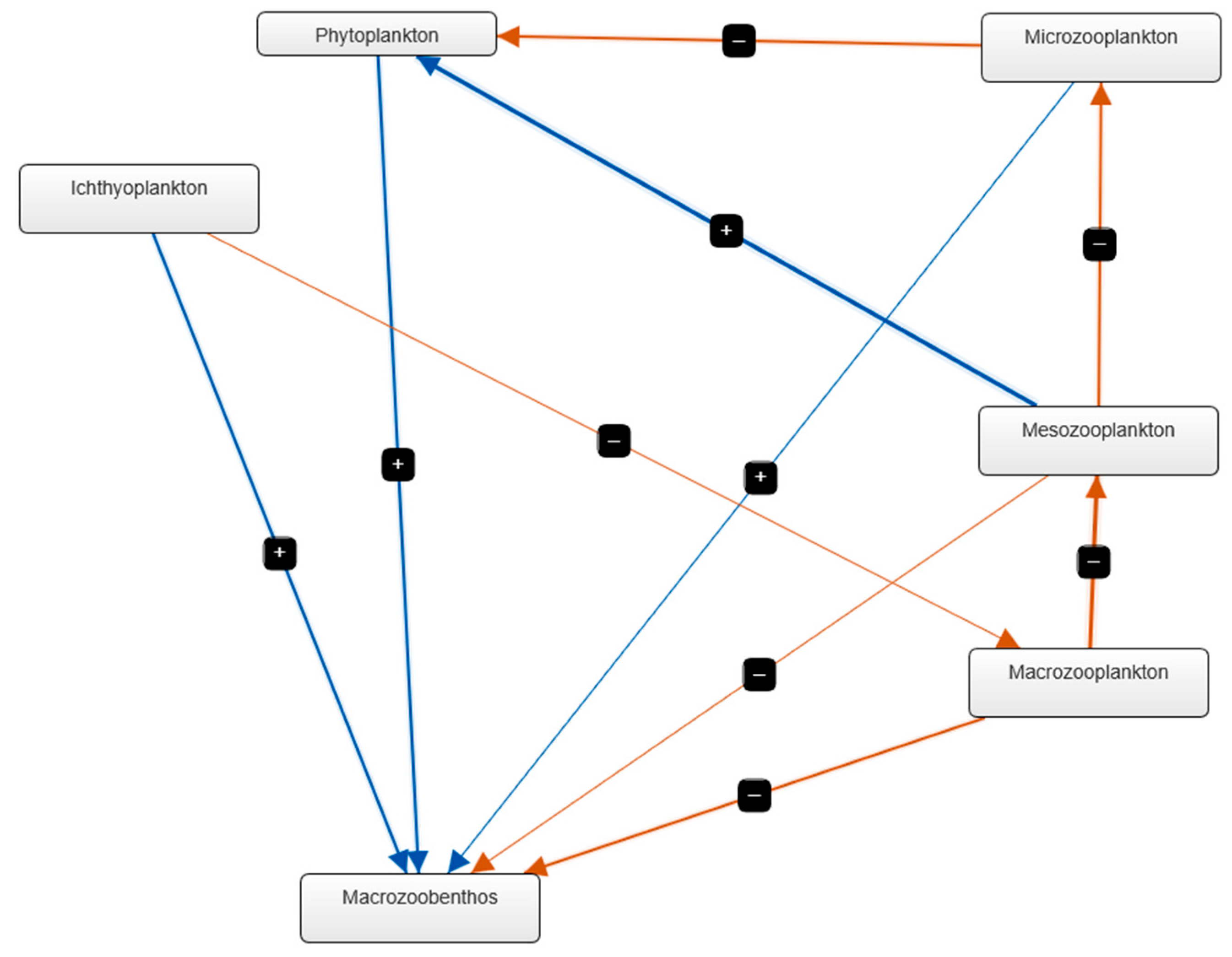
A Fuzzy Cognitive Map (FCM) of the coastal Black Sea food web was constructed based on correlation results [68]. Pearson correlation coefficients between trophic groups were used to define the direction and sign of FCM links. Positive correlations were interpreted as bottom-up or facilitative effects, while negative correlations indicated antagonistic or top-down interactions. The strength of trophic linkages was represented by arrow thickness proportional to correlation magnitude and significance. The adjacency structure was visualised using Mental Modeller [68].
Partial correlation analysis was applied to distinguish direct biological interactions from environmentally mediated effects [69]. Environmental variables were selected as control factors (Z) based on ecological relevance. Partial correlations were calculated as:
r x y z = r x y r x z r y z ( 1 r x z 2 ) ( 1 r y z 2 )
where rxy is the Pearson correlation between variables x and y, and rxz and ryz represent their correlations with the controlling variable Z.
Given the relatively small number of observations per sector, particularly in the central and southern areas, results should be interpreted with caution. Potential collinearity among variables was considered during PCA interpretation, particularly where variables exhibited similar loading patterns.

3. Results

The results presented below reflect patterns observed during a single survey conducted in June 2023 across a limited number of stations. Consequently, the identified spatial differences should be interpreted as indicative of the conditions within the studied area and period, rather than as representative of long-term or basin-wide dynamics in the Romanian Black Sea.

3.1. Environmental Parameters

Temperature exhibited moderate variability across sectors, with the northern area showing the widest range, whereas the central and southern sectors were more homogeneous, clustering around intermediate values (Table 1). Salinity displayed a clear north–south gradient, with the lowest and most variable values in the northern sector, and progressively higher, more stable conditions in the central and southern areas. Dissolved oxygen concentrations were generally high throughout the study area, although slightly reduced in the central sector compared to the northern and southern regions.
Nutrient distributions reflected strong spatial heterogeneity. Silicate, nitrate, nitrite, and total dissolved inorganic nitrogen (DIN) reached maximum concentrations in the northern sector, consistent with freshwater influence, while the central and southern areas showed markedly lower levels. Phosphate concentrations were low overall, with modest enrichment in the central sector, while ammonium exhibited elevated values in the northern and southern sectors and lower levels in the central area.
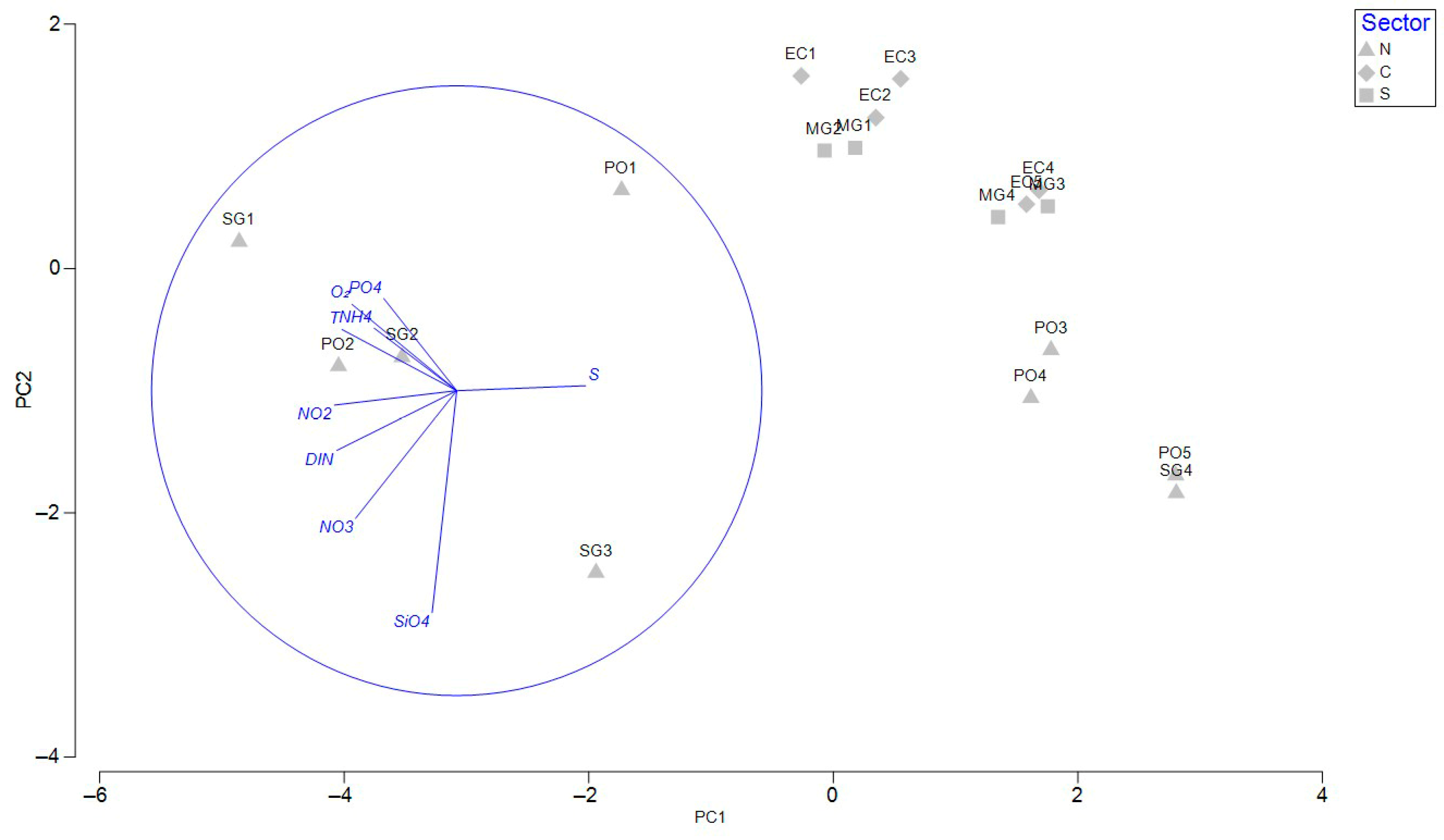
Principal Component Analysis (PCA) synthesized the observed environmental patterns, with the first two components explaining 76.1% of the total variance (PC1: 59.8%; PC2: 16.4%; eigenvalues = 5.38 and 1.48, respectively) (Figure 2; Table S2).
PC1 was primarily driven by salinity (positive loading: 0.423) and negatively associated with nutrient variables, including DIN (−0.393), nitrate (−0.332), nitrite (−0.401), and phosphate (−0.239), reflecting a gradient from nutrient-enriched freshwater-influenced conditions to more marine environments. PC2 was mainly defined by silicate (−0.728), nitrate (−0.419), and oxygen (0.283), indicating variability related to biogeochemical processes and water mass characteristics.
The projection of stations revealed a clear separation along PC1, with northern stations positioned on the negative side, associated with elevated nutrient concentrations, while central and southern stations clustered on the positive side, aligned with higher salinity. Along PC2, sectoral separation was less pronounced, although some northern stations showed associations with phosphate, ammonium, temperature, and dissolved oxygen.

3.2. Biotic Assemblages

3.2.1. Phytoplankton

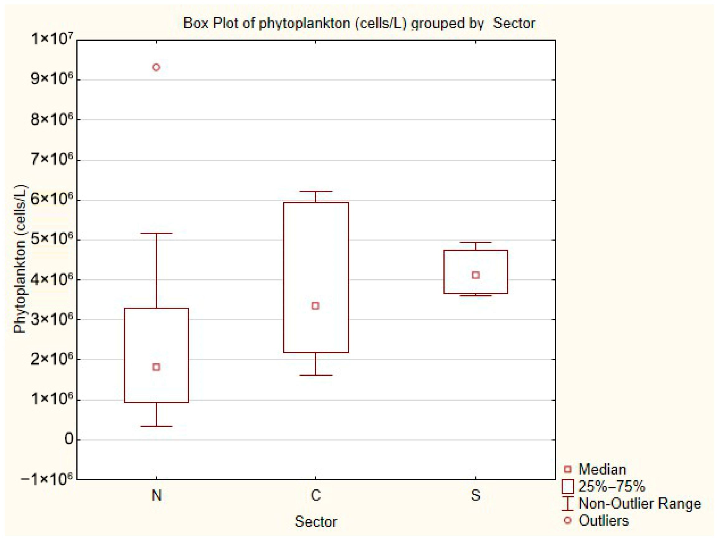
Phytoplankton abundance exhibited marked spatial differences among sectors (Figure 3). The northern sector showed the widest range, including very low concentrations alongside occasional extreme peaks, indicative of episodic bloom events. The central sector was characterised by higher median values and broader variability, suggesting more favourable conditions for phytoplankton growth. In contrast, the southern sector displayed the most homogeneous distribution, with abundances clustering within a narrower range at consistently elevated levels. This pattern highlights stronger fluctuations in the northern and central areas compared to the relatively stable phytoplankton community observed in the south. Overall, the data indicate greater variability and occasional blooms in the northern area, while the central sector shows moderately high values, and the southern sector maintains consistently elevated but less variable phytoplankton abundances.
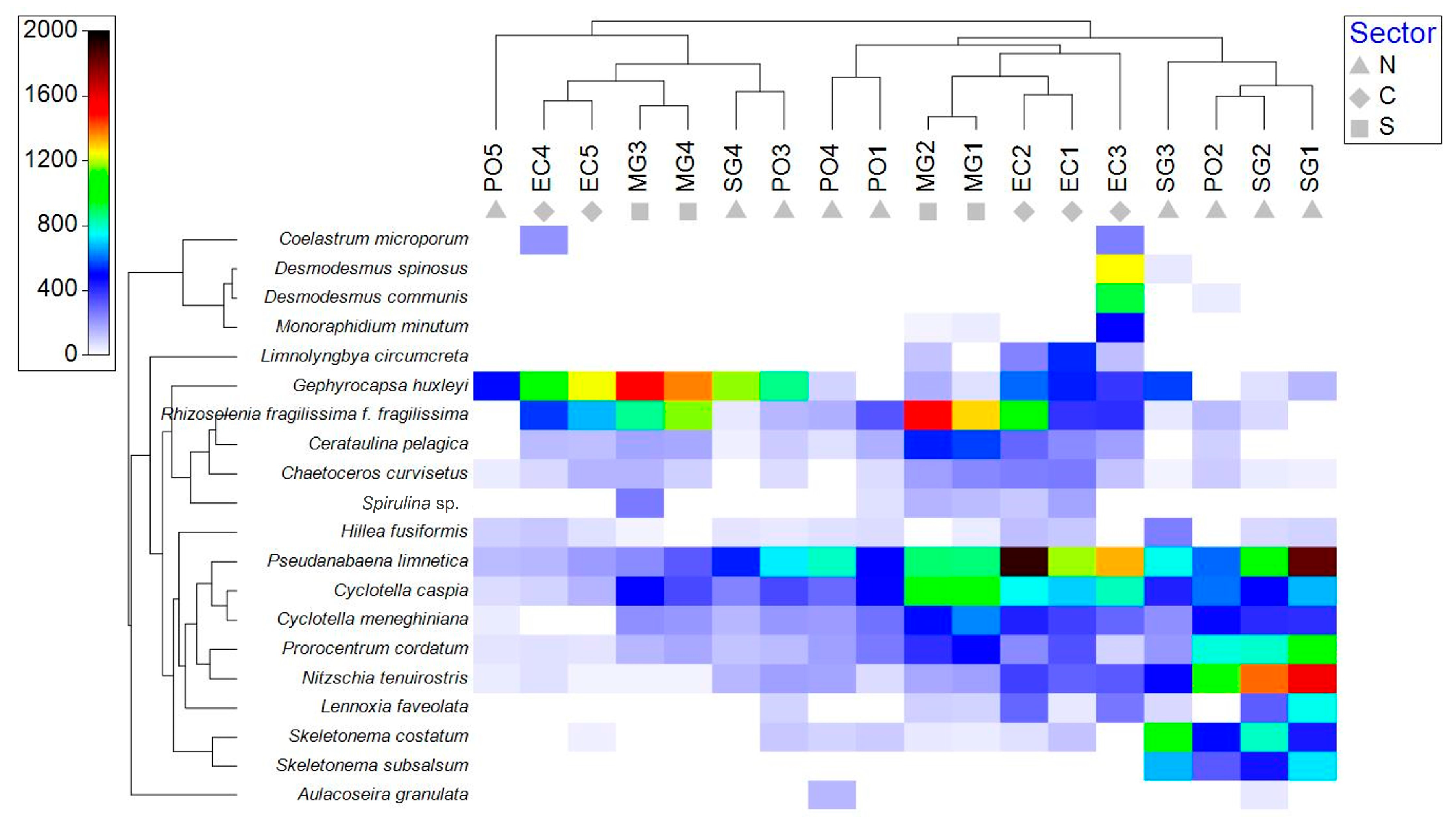
Phytoplankton diversity included 135 species (Table S3), of which 20 were dominant (Figure 4). Several phytoplankton blooms (over 1 million cells/L) were observed. The most extensive blooms (9.31 × 10⁶ cells/L) were recorded in the northern part, on 10 m isobath (SG 1 station), mainly driven by abundant growth of the cyanobacterium Pseudanabaena limnetica, the diatom species Nitzschia tenuirostris and the potentially toxic dinoflagellate Prorocentrum cordatum [70]. The cyanobacterium P. limnetica recorded the highest density on Est Constanta profile (station EC 2), together with the diatom species Rhizosolenia fragilissima f. fragilissima (station MG 2) in the southern part (Figure 4). High densities (5.92 × 10⁶ cells/L) have also been observed on the profile Est Constanta, at the EC 3 station, determined by some freshwater species, atypical for this area, such as P. limnetica and Desmodesmus spinosus (Figure 4).

3.2.2. Zooplankton

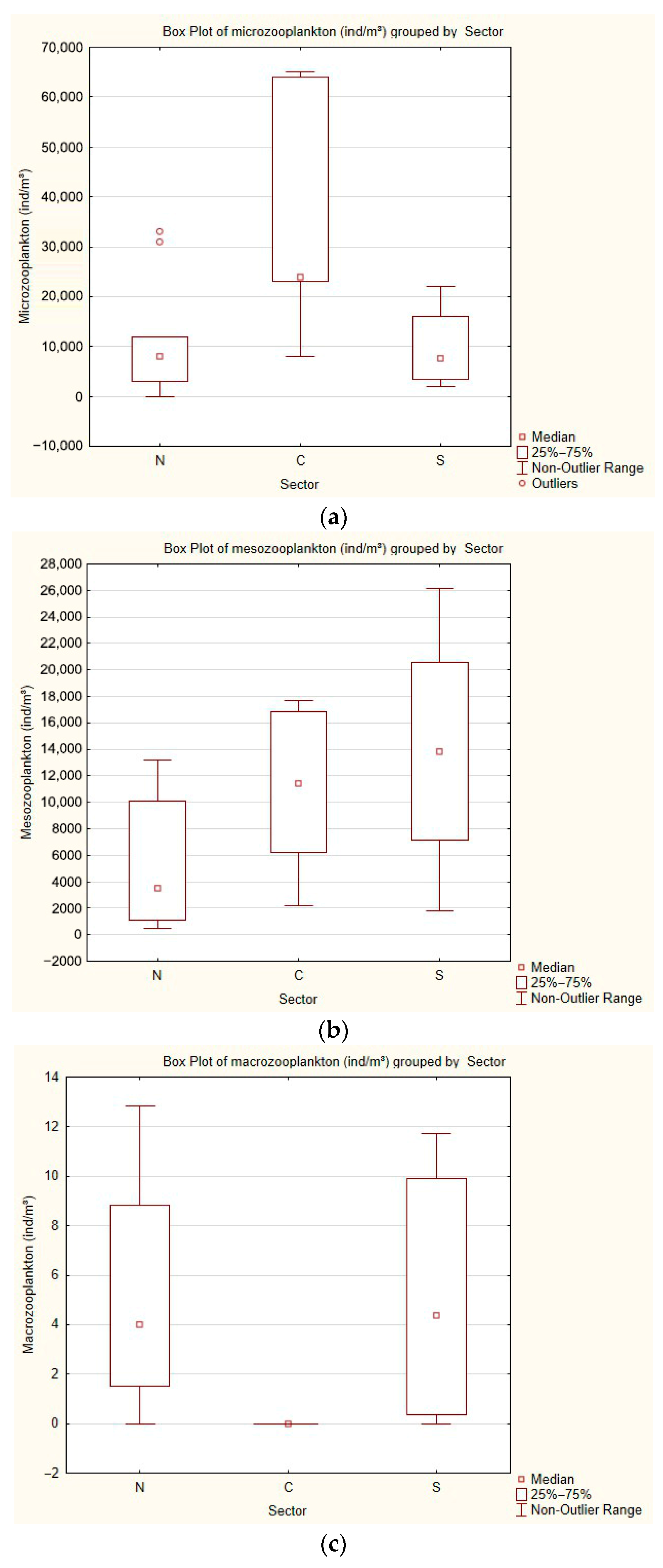
The three zooplankton components demonstrated divergent spatial organization: microzooplankton predominated in the central sector, mesozooplankton exhibited a progressive increase toward the south, and macrozooplankton occurred mainly in the northern and southern sectors, with minimal representation in the central area. This structuring underscores the contrasting ecological niches and distributional drivers shaping different trophic components of the zooplankton community.
Microzooplankton exhibited marked spatial differentiation, with the central sector supporting consistently higher abundances compared to the northern and southern areas. This central dominance was accompanied by broader variability, suggesting favorable conditions for microzooplankton proliferation. In contrast, the northern and southern sectors were characterized by comparatively reduced levels, although sporadic peaks in the north indicated localized enrichment events (Figure 5a).
Mesozooplankton displayed a clear latitudinal gradient. Abundances increased progressively from the northern to the southern sector, with the southern area sustaining the highest densities. The wider dispersion observed in this sector indicates both elevated baseline levels and episodic maxima, reflecting enhanced environmental suitability and potentially stronger coupling with regional productivity. The central sector occupied an intermediate position, showing moderate values relative to the two extremes (Figure 5b).
Macrozooplankton exhibited a contrasting distribution: the central sector was notably depleted, with abundances largely suppressed, while both the northern and southern sectors supported higher levels (Figure 5c). These latter regions were also marked by greater variability, indicating spatial heterogeneity and an uneven distribution across stations. The bimodal pattern suggests that macrozooplankton were preferentially associated with the peripheral sectors rather than the central waters.
Overall, the three zooplankton components demonstrated divergent spatial organization: microzooplankton predominated in the central sector, mesozooplankton increased steadily toward the south, and macrozooplankton was concentrated in the northern and southern areas.
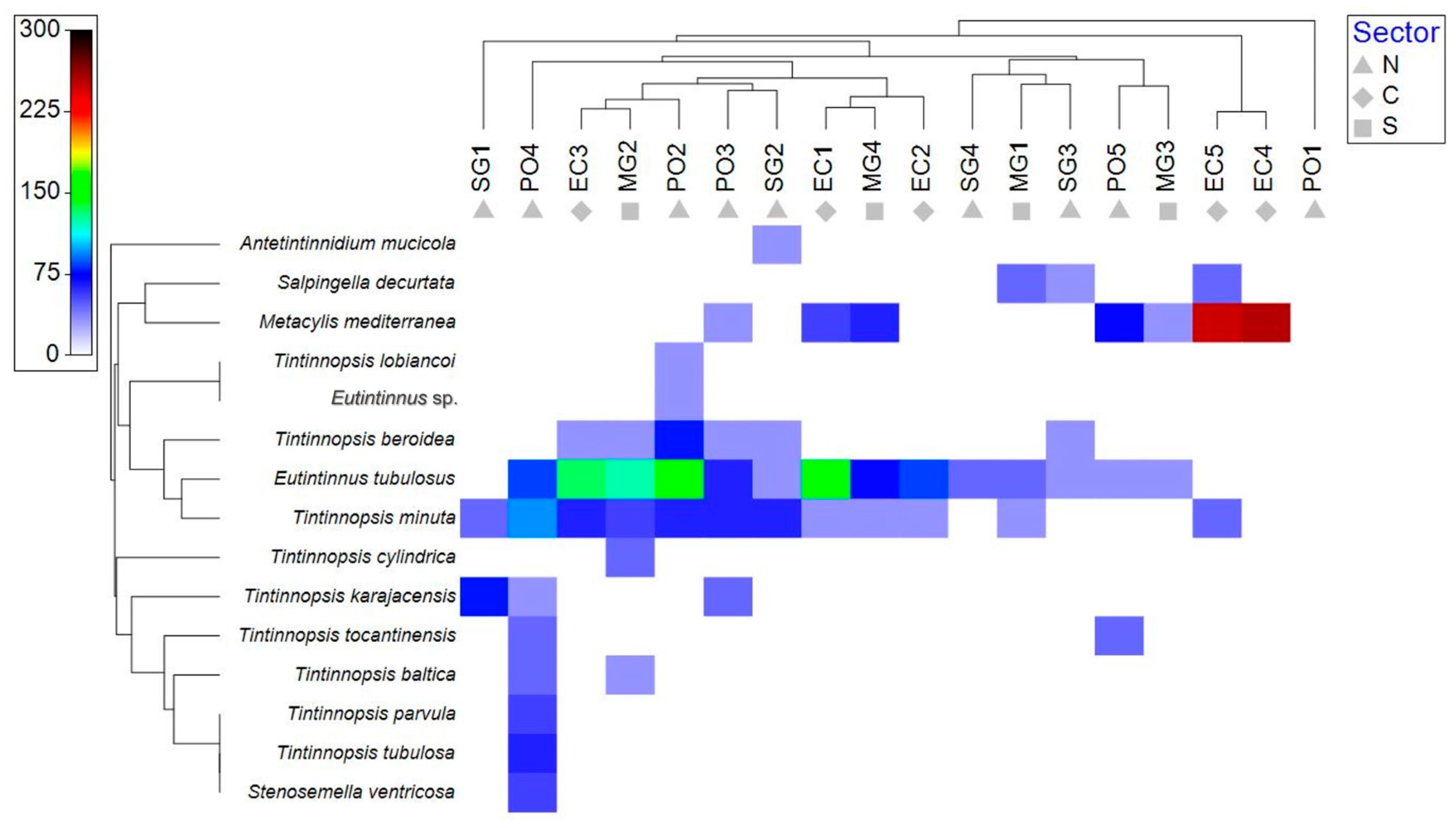
The tintinnids from microzooplankton are dominated by the genus Tintinnopsis, Eutintinnus and Metacylis, which form long, coherent high-intensity bands (Figure 6). Peak densities occur at EC4 and EC5, with secondary maxima at PO2; signals attenuate sharply along the PO/SG plume transect and are sporadic at southern/coastal stations (MG2). The station dendrogram (Bray–Curtis; average linkage) isolates the EC station, indicating a mid-shelf maximum and a consistent microzooplankton response to the shelf hydrographic regime.
Shade plot and clustering analysis showed clear spatial variation in tintinnid assemblages (Figure 6). Eutintinnus tubulosus and Tintinnopsis minuta were the most widespread and abundant species, while Metacylis mediterranea reached a distinct peak at marine waters of a central sector. Several species occurred sporadically in low densities, and Eutintinnus sp., Tintinnopsis lobiancoi and Antetintinnidium mucicola appeared only once. Station clustering grouped central offshore stations EC4 and EC5 (with 83.81 similarity), while southern and northern stations were more heterogeneous. SG1, PO1 and PO4 were out of the rest of the stations. In PO1, no tintinnids were identified, while the highest species diversity was recorded at station PO4.
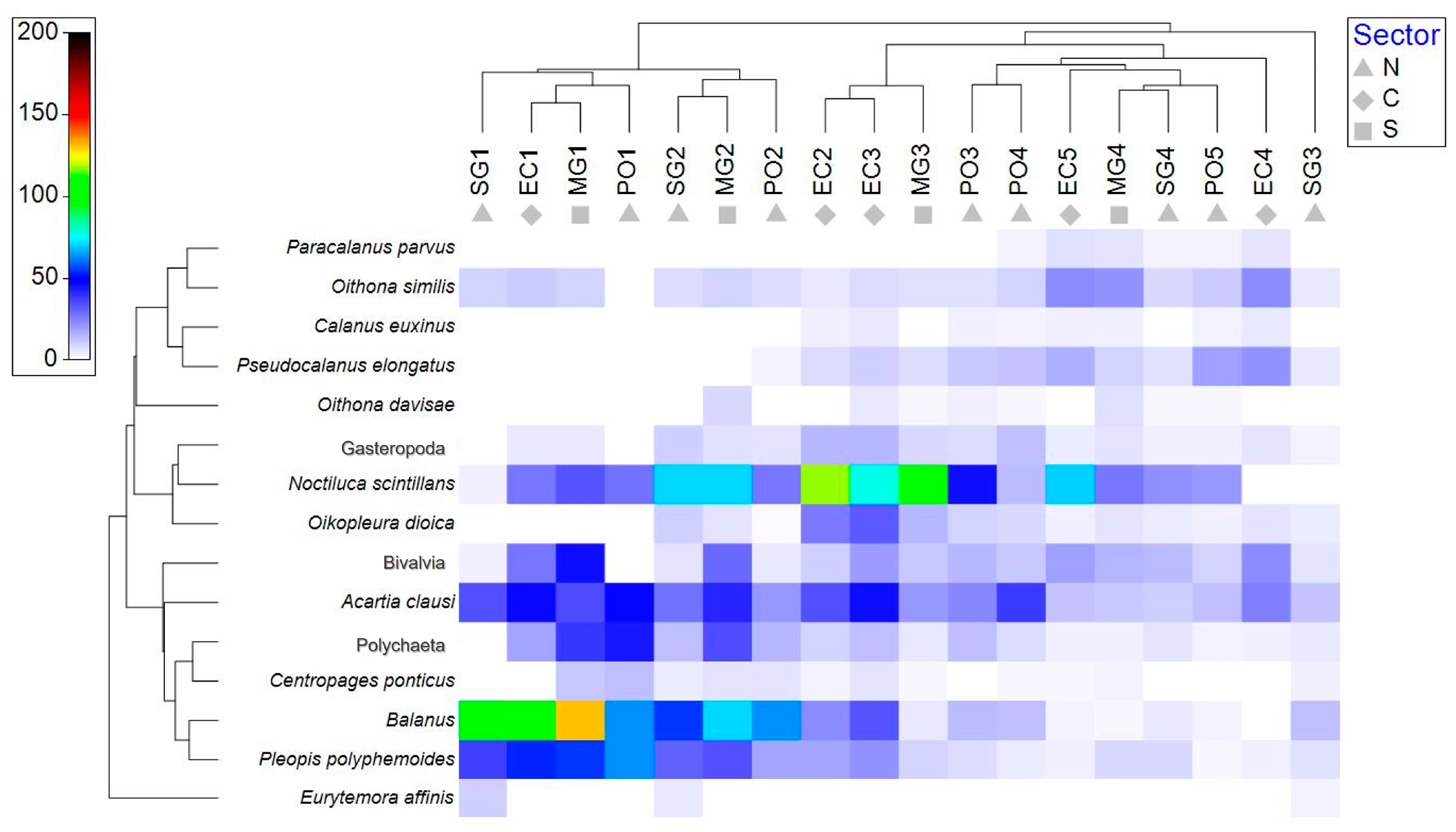
The shade plot revealed marked differences in mesozooplankton community structure among stations (Figure 7). Acartia clausi and Pleopis polyphemoides were consistently present and often abundant, while Balanus larvae reached peak values at EC1. Noctiluca scintillans and Oikopleura dioica showed localized blooms, whereas copepods such as Paracalanus parvus, Calanus euxinus, and Oithona spp. were generally less abundant. Station clustering grouped northern and central sites, while several southern stations formed separate clusters, indicating spatial heterogeneity driven by species dominance patterns.
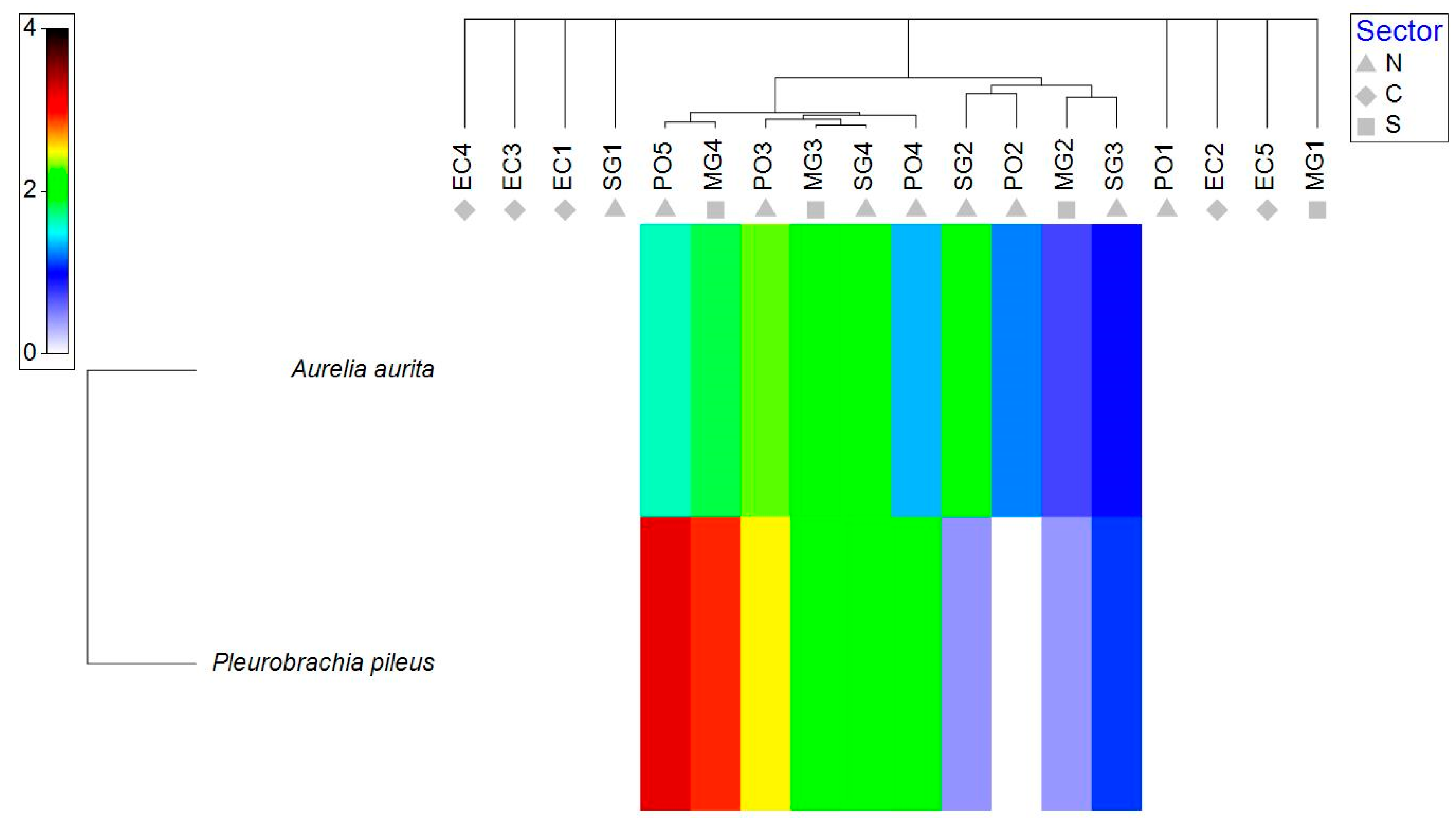
Macrozooplankton communities were dominated by Aurelia aurita and Pleurobrachia pileus, which exhibited contrasting distributional patterns (Figure 8). A. aurita was broadly present at moderate densities across most stations, whereas P. pileus showed pronounced localized peaks, particularly at PO5. The station clustering reflected these differences, separating sites dominated by P. pileus from those where A. aurita prevailed, highlighting the spatial heterogeneity of gelatinous assemblages along the coast.

3.2.3. Ichthyoplankton

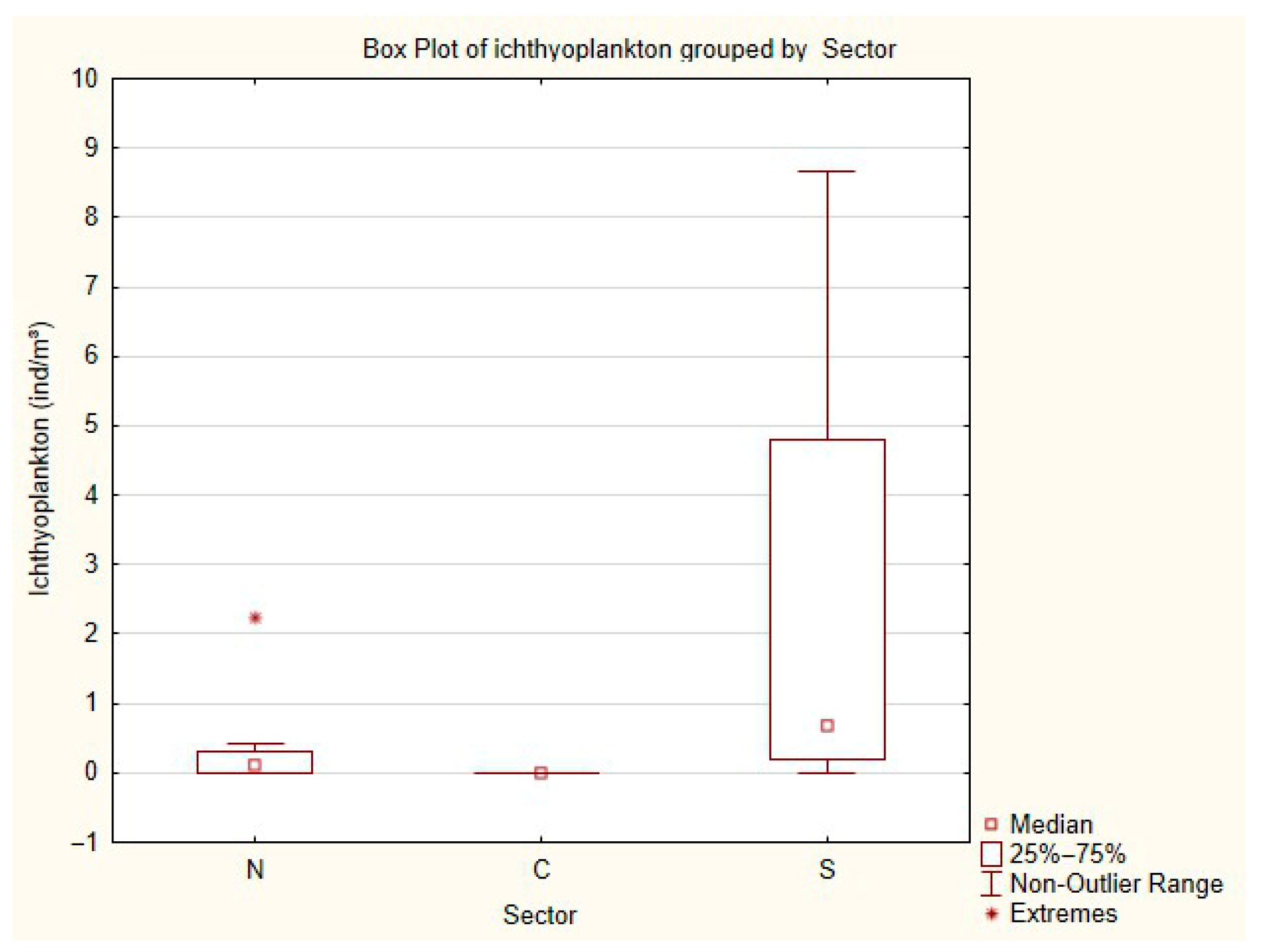
Ichthyoplankton exhibited pronounced spatial contrasts across sectors. The central sector was largely devoid of individuals, while the northern sector supported only very low levels, with a single exceptional value indicating localized occurrence (Figure 9). By contrast, the southern sector sustained the highest abundances, with both elevated medians and wider variability compared to the other regions. This distribution suggests that ichthyoplankton were concentrated primarily in the southern waters, with marginal presence in the northern sector and near absence from the central area.
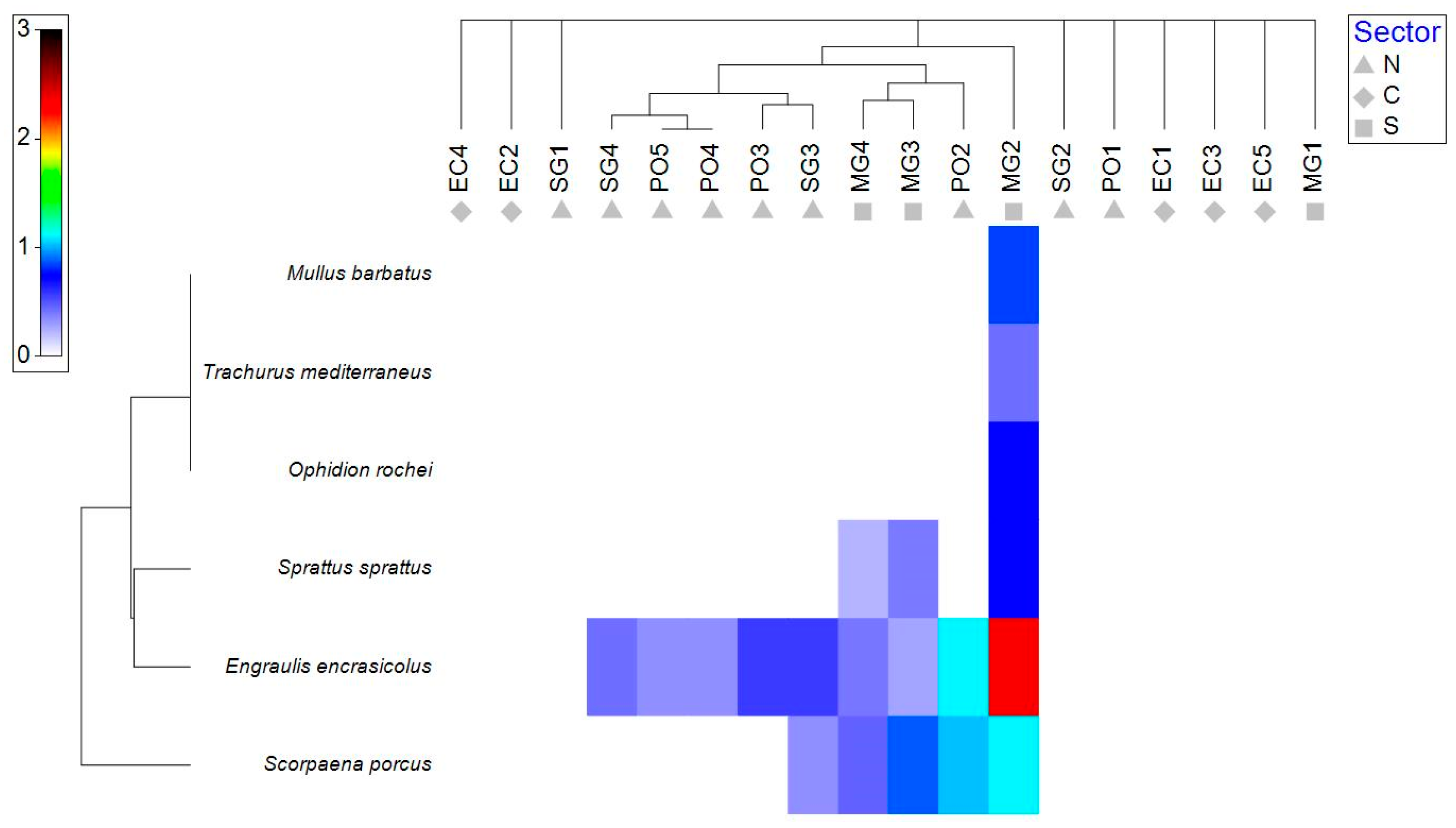
The ichthyoplankton assemblage was represented mainly by Engraulis encrasicolus, Sprattus sprattus, and Scorpaena porcus, with localized contributions from Mullus barbatus, Trachurus mediterraneus, and Ophidion rochei (Figure 10). The highest densities were recorded for E. encrasicolus and S. porcus, particularly at MG2 and PO2, while other species occurred sporadically at low levels. Station clustering reflected these dominance patterns, separating sites with abundant clupeiformes larvae from those characterized by scarce or absent ichthyoplankton, emphasizing the patchy distribution of early fish life stages along the coast.

3.2.4. Macrozoobenthos

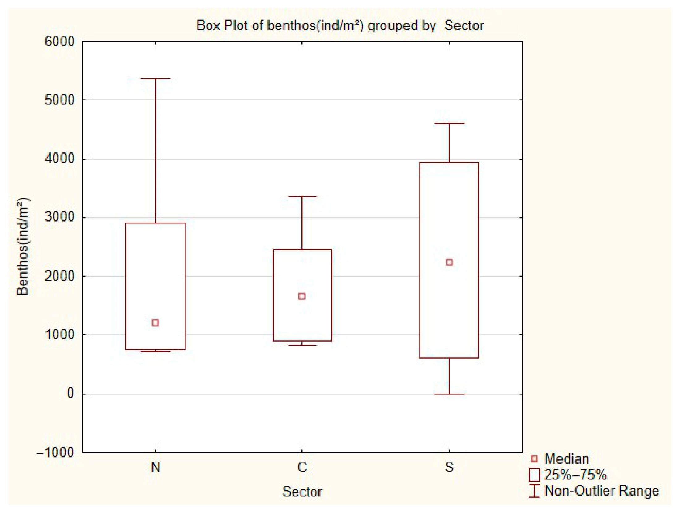
The macrozoobenthos displayed relatively high variability across all sectors, with clear differences in distributional patterns. The northern and central sectors showed comparable abundance levels, although the northern sector exhibited a wider spread, indicating stronger heterogeneity among sampling stations (Figure 11). The central sector was more homogeneous, with abundances clustered around intermediate values. The southern sector sustained the highest overall abundances, but also the broadest variability, ranging from very low to markedly elevated levels. This suggests that benthic macrofauna communities were more developed in the southern area, while the northern and central regions supported more moderate but less variable populations.
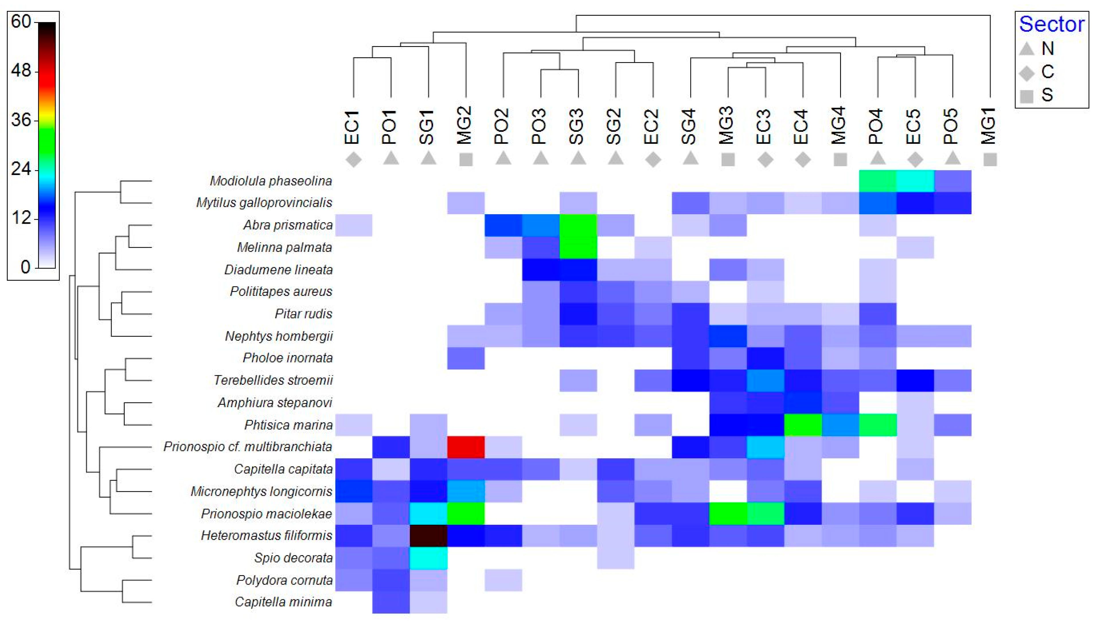
Macrozoobenthos diversity included 112 species dominant (Table S2), of which 20 were dominant (Figure 12). The benthic macrofauna assemblages were dominated by polychaetes such as Heteromastus filiformis, Prionospio cf. multibranchiata, and Capitella capitata, along with bivalves (Modiolula phaseolina, Abra prismatica) and amphipods (Ampelisca ssp.) (Figure 12). High densities of C. capitata and Polydora cornuta were observed in several central and northern stations, whereas P. multibranchiata and H. filiformis showed localized peaks. Cluster analysis grouped stations by the prevalence of opportunistic versus sensitive taxa, reflecting spatial heterogeneity in zoobenthic community structure across the sectors.
Absolute abundance ranges of planktonic and benthic groups varied across sectors (Table S4). Phytoplankton abundance ranged from 334,120 to 9,313,600 cells/L in the northern sector, 1,614,000 to 6,232,000 cells/L in the central sector, and 3,615,840 to 4,931,380 cells/L in the southern sector.
Microzooplankton ranged from 0 to 33,000 ind/m3 in the north, 8000 to 65,000 ind/m3 in the central sector, and 2000 to 22,000 ind/m3 in the south. Mesozooplankton ranged from 456 to 13,190 ind/m3 in the northern sector, 2223 to 17,658 ind/m3 in the central sector, and 1777 to 26,133 ind/m3 in the southern sector.
Macrozooplankton showed low but variable abundances, ranging from 0 to 12.ind/m3 in the north, being absent in the central sector, and reaching up to 11.74 ind/m3 in the south. Ichthyoplankton was generally scarce, ranging from 0 to 2.25 ind/m3 in the northern sector, absent in the central sector, and reaching up to 8.66 ind/m3 in the southern sector.
Macrozoobenthos abundance ranged from 710 to 5360 ind/m2 in the northern sector, 820 to 3360 ind/m2 in the central sector, and 0 to 4600 ind/m2 in the southern sector.
Differences among sectors were assessed using the Kruskal–Wallis test. Significant differences were observed for macrozooplankton (H = 6.67, p = 0.036) and ichthyoplankton (H = 6.81, p = 0.033), while other groups did not show statistically significant variation among sectors (p > 0.05), despite evident spatial trends (Table S5).

3.3. Interrelations Between Biotic and Abiotic Components

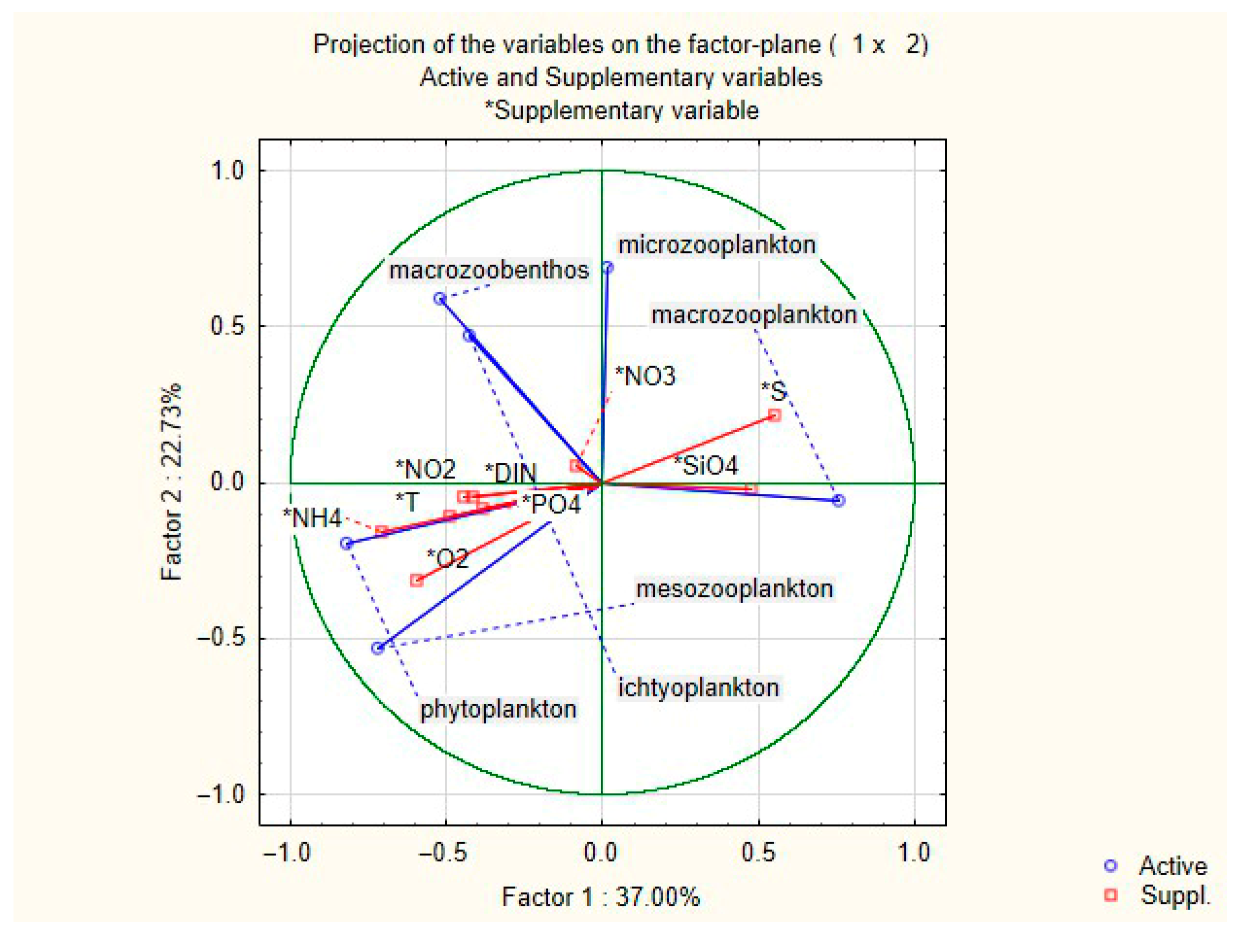
Multivariate analyses highlighted strong associations between environmental gradients and food-web components. The PCA explained 59.7% of total variance on the first two axes (Factor 1: 37.0%; Factor 2: 22.7%) (Figure 13). Along Factor 1, salinity and silicate loaded positively together with macrozooplankton, while nitrate, nitrite, and DIN loaded negatively with microzooplankton. This separation reflects the contrast between saline, marine-influenced southern waters, where gelatinous taxa were more abundant, and nutrient-enriched northern waters, which sustained microzooplankton populations linked to phytoplankton blooms. Factor 2 separated macrozoobenthos and ichthyoplankton on the positive side from phytoplankton and mesozooplankton on the negative side, the latter associated with oxygen, ammonium, phosphate, and temperature. This arrangement indicates that mesozooplankton responded closely to water-column productivity, while macrozoobenthos and ichthyoplankton reflected broader ecosystem conditions.
Correlation analysis reinforced these patterns (Table 2). In the north, phytoplankton and mesozooplankton correlated strongly with DIN and ammonium, highlighting nutrient-driven production, whereas macrozooplankton aligned positively with salinity and silicate and negatively with oxygen, consistent with marine influence and patchy gelatinous dominance. In the central sector, phytoplankton related to oxygen and phosphate, suggesting links to localized productivity, while mesozooplankton correlated with nitrite and oxygen. Microzooplankton, by contrast, were associated with salinity, indicating a distinct niche. In the south, phytoplankton and ichthyoplankton correlated tightly with ammonium and DIN, pointing to efficient coupling of nutrient supply with larval fish prey availability. Macrozooplankton showed consistent positive associations with salinity and silicate, reflecting their prevalence in more marine conditions.
Taken together, the multivariate analysis results demonstrate that nutrient enrichment supported plankton dynamics in the northern and southern sectors, while oxygen and phosphate shaped community structure in the central sector. The north was characterized by short, nutrient-fuelled pathways from phytoplankton to microzooplankton, while the south sustained more extended trophic connections, linking phytoplankton through mesozooplankton to ichthyoplankton. Macrozooplankton tracked saline, silicate-rich waters throughout, often decoupled from nutrient dynamics, whereas macrozoobenthos exhibited weaker but spatially variable correlations with environmental factors.

3.4. Interaction Between Biotic Assemblages

The analysis indicates that only two interactions within the matrix are statistically significant, revealing a focused trophic cascade within the system (Table 3). A significant positive correlation was observed between phytoplankton and mesozooplankton (0.514), indicating a close coupling between primary producers and their consumers. This relationship is interpreted ecologically as bottom-up support of mesozooplankton by phytoplankton, consistent with established trophic dynamics, although correlation analysis alone does not imply direct causality or interaction direction. Conversely, macrozooplankton exert a significant negative effect on mesozooplankton (−0.570), indicating strong top-down control. All remaining interaction coefficients were not statistically significant, implying that their contributions to system structure are comparatively weak or inconsistent. Overall, the results point to a simplified core dynamic dominated by the macrozooplankton–mesozooplankton–phytoplankton linkage, which emerges as the primary driver of variability in the modelled food-web interactions.
The Fuzzy Cognitive Map (FCM) (Figure 14) integrates all pairwise correlations among trophic components and highlights the relatively small number of statistically significant interactions that structure the system (Table 3). The strongest relationship is the negative influence of macrozooplankton on mesozooplankton (−0.570), indicating pronounced top-down control on intermediate consumers. In contrast, a positive relationship between phytoplankton and mesozooplankton reflects bottom-up support of primary producers for zooplankton development.
Together, these significant pathways identify macrozooplankton as key regulators of mesozooplankton dynamics, while phytoplankton represent the primary resource base sustaining mesozooplankton productivity. Although the FCM includes all interactions, most remaining connections are weak and not statistically significant, suggesting more variable or indirect ecological linkages such as grazing, competition, and benthic–pelagic coupling. Overall, the network structure indicates that the system is primarily shaped by the combined influence of top-down control from macrozooplankton and bottom-up energy input from phytoplankton.
The structural indices (Table 4) show that phytoplankton act as the main driver in the network, exerting influence without receiving inputs, while benthos functions as a pure receiver, with the highest indegree and no outgoing effects. The remaining components are ordinary nodes with mixed influence patterns, among which mesozooplankton display the greatest centrality, indicating its prominent role in mediating trophic interactions.
Partial correlation analysis (Table 5) revealed that, in the phytoplankton–mesozooplankton relationship, phytoplankton biomass exhibited a strong positive correlation with NH4, while mesozooplankton showed a similarly strong association with the same nutrient. Both relationships exceeded the direct correlation observed between phytoplankton and mesozooplankton (r = 0.514), indicating that NH4 represents a major underlying driver influencing both trophic groups. This pattern suggests that nutrient enrichment may artificially strengthen the apparent phytoplankton–mesozooplankton coupling, thereby supporting the selection of NH4 as the controlling variable in the partial correlation analysis.
For the macrozooplankton–mesozooplankton pair, both groups were significantly associated with salinity, albeit in opposite directions. Macrozooplankton exhibited a positive correlation with salinity, whereas mesozooplankton displayed a moderate negative association. Importantly, the persistence of a strong negative partial correlation after controlling for salinity indicates that this interaction is not primarily mediated by environmental gradients. Instead, it likely reflects a direct biological interaction, such as predation or suppressive pressure exerted by macrozooplankton on mesozooplankton.

4. Discussion

4.1. Environmental Parameters

The June 2023 survey highlighted pronounced environmental gradients across the Romanian Black Sea coastal sectors. While temperature remained relatively uniform, salinity revealed a steep north–south gradient, influenced by substantial freshwater discharge from the Danube in the north and more marine conditions to the south [71].
This gradient appeared broadly continuously at the regional scale; however, it is likely modulated by localized freshwater plumes and mesoscale circulation features, which can create patchiness in salinity distribution, particularly in the northern and mid-shelf areas. The influence of the Danube plume is known to be highly dynamic, with its spatial extent and direction depending on river discharge, wind forcing, and coastal currents [72]. As a result, the salinity structure observed during this survey represents a snapshot of conditions during early summer and may vary seasonally [73]. Increased river discharge during spring or episodic events (e.g., flooding) can intensify freshwater spreading, while reduced discharge or stronger stratification in summer may limit its extent [44,74].
These salinity patterns play a key role in structuring planktonic and benthic communities [75,76], but their temporal variability should be considered when interpreting spatial patterns observed in short-term surveys.
Silicate showed pronounced spatial variability, with maximum concentrations in the northern sector and a marked decline toward southern areas. This pattern is consistent with the influence of Danube-derived freshwater inputs, which are a major source of dissolved silicate in the northwestern Black Sea [72].
The exceptionally high silicate concentrations observed during this study may also be linked to recent hydrological disturbances, including the Nova Kakhovka dam breach, which occurred in early June 2023, shortly before the sampling period. This event likely enhanced the downstream transport of suspended material and nutrients, potentially contributing to elevated silicate levels in coastal waters [25,77]. However, given the timing and spatial complexity of plume dispersal, this influence should be interpreted with caution, as the relative contribution of Danube discharge versus episodic inputs cannot be fully disentangled.
Compared to previous studies in the region, the silicate concentrations recorded here fall within the upper range of reported values, although peak concentrations in the northern sector appear elevated relative to typical background conditions [25,44,78]. Elevated silicate availability likely supports diatom productivity and may propagate through the food web, influencing higher trophic levels such as tintinnids and copepods [79,80].
Nutrients such as nitrate and nitrite were similarly elevated in the north, reflecting freshwater-driven enrichment [72,81], while the central and southern sectors were oligotrophic [82]. Ammonium peaks in both northern and southern sectors may relate to localised benthic regeneration, and anthropogenic impact, and the pervasive low phosphate suggests a potential phosphorus limitation consistent with recent regional trends [39,83].
The PCA reinforced these patterns, with PC1 clearly separating nutrient-rich northern stations from more saline and comparatively nutrient-poor southern ones. This separation reflects the dominant influence of Danube freshwater inputs and the mixing between riverine and marine waters, generating a gradient from eutrophic, low-salinity conditions in the north to more oligotrophic marine conditions in the south [84,85]. This gradient is further modulated by hydrodynamic processes, including coastal circulation and plume dispersion, which control the transport and dilution of riverine inputs across the shelf [86].
PC2 captured secondary variability associated with phosphate, ammonium, and dissolved oxygen, likely linked to biogeochemical cycling processes such as organic matter remineralisation, phytoplankton uptake, and microbial activity. Variability along this axis reflects localised ecosystem processes rather than large-scale physical forcing.
Overall, these results highlight the combined role of freshwater inputs, mixing dynamics, and internal biogeochemical processes in structuring environmental gradients across the Romanian Black Sea shelf. These gradients not only define physicochemical conditions but also influence trophic organisation, with nutrient-enriched northern waters supporting more dynamic, potentially pulsed production systems and southern areas reflecting more stable, marine-dominated conditions [7].

4.2. Biotic Assemblages

  • Phytoplankton
Phytoplankton formed the energetic base of the pelagic food web and showed clear spatial contrasts across sectors (Figure 3). In the northern area, abundances fluctuated strongly, ranging from very low concentrations to episodic blooms exceeding 106 cells L−1. Such events were dominated by cyanobacteria (P. limnetica), diatoms (N. tenuirostris, R. fragilissima f. fragilissima), and dinoflagellates (P. cordatum), consistent with earlier observations of opportunistic bloom taxa in Danube-influenced waters [25,75]. The occurrence of the potentially toxic dinoflagellate P. cordatum is ecologically significant, as this species is commonly associated with eutrophic and stratified conditions and has been linked to harmful algal bloom events in the Black Sea and other coastal systems [87,88,89]. Its presence suggests that local environmental conditions may favour bloom-forming taxa capable of altering trophic dynamics, including reduced grazing efficiency and modified energy transfer to higher trophic levels [10,90]. The central sector exhibited moderately high values with broad variability, suggesting more stable yet productive conditions, while the southern area supported consistently elevated abundances with reduced variability, dominated by large-celled diatoms such as R. fragilissima f. fragilissima and Cerataulina pelagica. The north–south gradient reflects the influence of freshwater-driven silicate enrichment in the north [72,91] and more saline, oligotrophic waters in the south [92]. These contrasting phytoplankton patterns may suggest differences in the temporal availability and composition of primary production across sectors, with episodic variability in the north and more consistent conditions in the south. However, given the limited temporal scope of the study, these observations should be interpreted cautiously.
The apparent discrepancy between nutrient levels and phytoplankton abundance patterns highlights the complex and non-linear nature of phytoplankton dynamics [93]. Although nutrient concentrations were highest in the northern sector, phytoplankton biomass exhibited high variability, reflecting episodic bloom events rather than sustained production. In contrast, the central sector, despite intermediate nutrient levels, showed higher median phytoplankton abundance, likely due to more stable environmental conditions that support sustained growth. The relatively homogeneous phytoplankton levels in the southern sector further suggest consistent trophic conditions, where lower variability in environmental drivers may promote steady biomass. These patterns indicate that phytoplankton distribution is influenced not only by nutrient availability but also by physical stability, grazing pressure, and temporal dynamics.
  • Zooplankton
The zooplankton community exhibited a clear structuring into micro-, meso-, and macrozooplankton components, each responding differently to environmental conditions and phytoplankton availability. Microzooplankton, particularly tintinnids (Eutintinnus, Tintinnopsis, Metacylis), formed dense mid-shelf maxima in the central sector, where nutrient inputs and phytoplankton peaks created favourable conditions. Their role as primary grazers of small phytoplankton and bacteria and as prey for mesozooplankton and larval fish underscores their central position in the microbial loop [16,94,95]. Mesozooplankton showed a latitudinal increase, with highest abundances in the southern sector, dominated by copepods (A. clausi, P. polyphemoides) and punctuated by localised blooms of N. scintillans and appendicularians (O. dioica). This distribution aligns with more stable phytoplankton conditions and favourable hydrography in the south, enhancing the transfer of energy to planktivorous fish [96,97]. Macrozooplankton, mainly gelatinous taxa such as Aurelia aurita and P. pileus, showed contrasting distributions: A. aurita was broadly distributed at moderate levels, while P. pileus exhibited localised peaks, especially at PO5. Their presence highlights a recurring feature of the Black Sea food web, where gelatinous organisms compete with fish for zooplankton prey and occasionally exert strong top-down control [7,28,98].
  • Ichthyoplankton
The distribution of fish larvae further emphasised the trophic coupling between plankton production and higher consumers. The central sector was largely devoid of ichthyoplankton, while the northern sector supported only low levels, occasionally punctuated by localised maxima. In contrast, the southern sector sustained the highest abundances, dominated by clupeids (E. encrasicolus and S. sprattus) and supplemented by species such as S. porcus, M. barbatus, T. mediterraneus, and O. rochei. The spatial overlap between abundant mesozooplankton in the south and ichthyoplankton peaks suggests strong bottom-up control, where prey availability determines recruitment success [99,100]. This emphasises the role of southern waters as key nursery areas, sustained by stable phytoplankton–zooplankton production and favourable hydrographic conditions.
The coexistence of high mesozooplankton and predator abundances in the southern sector suggests that additional environmental factors may contribute to sustaining elevated prey biomass despite grazing pressure. In particular, stable hydrodynamic conditions, including reduced turbulence and the influence of coastal currents, may promote the retention and accumulation of zooplankton in this region [26,101]. Enhanced food availability, driven by relatively consistent phytoplankton production, may further support rapid zooplankton growth, compensating for predation losses.
Moreover, coastal circulation patterns may facilitate the aggregation of planktonic organisms and create localised hotspots of productivity, reinforcing trophic coupling [102]. These combined effects highlight the importance of physical–biological interactions in structuring zooplankton distributions and sustaining productive nursery areas in the southern Black Sea.
  • Macrozoobenthos
Macrozoobenthic assemblages reflected habitat diversity and contributed to benthic–pelagic coupling. Highest densities were recorded in infralittoral habitats of the northern and southern sectors, where opportunistic polychaetes (C. capitata, Prionospio maciolekae, H. filiformis) dominated, reflecting eutrophic conditions and organic matter enrichment [103]. However, it should be noted that sediment organic content and oxygen conditions were not directly measured in this study; therefore, this interpretation remains indicative and should be confirmed by future investigations incorporating benthic geochemical parameters. Circalittoral habitats (≤45 m) supported moderate densities of polychaetes and crustaceans, while deeper circalittoral zones (>45 m) were dominated by molluscs and amphipods. Biomass was highest in the southern coastal waters, driven by polychaetes and bivalves (Chamelea gallina), while northern sites were characterised by Mytilus galloprovincialis and other suspension-feeding bivalves. These benthic communities provide prey for demersal fish and contribute to nutrient recycling, influencing phytoplankton dynamics and closing the loop between benthic and pelagic compartments [104].
The assemblages highlight a food web shaped by environmental gradients and sectoral contrasts. Episodic nutrient pulses in the north, particularly silicate, fuelled short-lived diatom and cyanobacteria blooms, which cascaded to microzooplankton but did not consistently propagate to higher trophic levels. In contrast, the southern sector supported more stable diatom–mesozooplankton–fish larvae linkages, indicating efficient energy transfer along the food chain. Gelatinous zooplankton intermittently disrupted this flow by competing with fish for prey, while benthic communities recycled organic matter and provided additional food sources for demersal fish. These patterns underscore the complex interactions and spatial heterogeneity of the Black Sea food web, where environmental forcing and trophic interactions jointly determine ecosystem functioning.
Overall, the observed patterns are consistent with previous studies from the Black Sea, where biotic assemblages are strongly structured by environmental gradients, particularly freshwater input, nutrient availability, and hydrodynamic conditions [4,7]. The high variability and episodic phytoplankton blooms recorded in the northern sector reflect persistent Danube influence and eutrophic conditions, favouring opportunistic taxa, while the more stable diatom-dominated communities in the southern sector are associated with marine conditions and reduced environmental variability.
The increase in mesozooplankton and ichthyoplankton abundance toward the southern sector aligns with studies highlighting the importance of hydrographic stability and retention processes in sustaining trophic transfer efficiency [30,102,105,106]. At the same time, the occurrence of gelatinous macrozooplankton reflects broader ecosystem shifts in the Black Sea, where these taxa can alter trophic pathways and reduce energy transfer to higher consumers [107,108,109].
The dominance of opportunistic benthic taxa in nutrient-influenced areas is also consistent with previous findings linking benthic community structure to organic enrichment and disturbance [110,111,112,113,114,115]. Together, these results highlight a spatially heterogeneous system in which environmental forcing and trophic interactions jointly shape ecosystem functioning. However, these findings represent a snapshot of summer conditions and should be interpreted cautiously, given the strong seasonal variability characteristic of the Black Sea.

4.3. Environmental Control and Food-Web Linkages

The multivariate analyses showed that the structure of biotic assemblages was strongly shaped by spatially heterogeneous environmental gradients along the Romanian coast. In the northern sector, phytoplankton and mesozooplankton correlated positively with DIN and ammonium, highlighting the role of nutrient enrichment in fuelling pelagic production. Such nutrient-driven responses are expected under Danube influence, which supplies large nitrogen loads to the coastal zone [72,81]. The positive association of phytoplankton with nitrate and ammonium, combined with strong mesozooplankton–oxygen coupling, suggests that episodic blooms generated rapid trophic transfer toward copepods, consistent with short, pulsed food-web pathways. In contrast, macrozooplankton in the north correlated positively with salinity and silicate but negatively with oxygen, reflecting conditions less influenced by riverine inputs and more by marine intrusions. The negative association with oxygen may be related to the higher tolerance of gelatinous taxa to low-oxygen or variable oxygen conditions compared to many crustacean zooplankton. Such conditions may reduce competition and predation pressure, thereby favouring gelatinous organisms. This pattern is consistent with previous studies showing that gelatinous zooplankton can proliferate under environmentally stressed or hypoxic conditions, where they may reduce the efficiency of trophic transfer [7,28].
In the central sector, correlations pointed to a different structuring mechanism. Phytoplankton were positively related to oxygen and phosphate, while mesozooplankton were linked to nitrite and oxygen. Microzooplankton, by contrast, were associated with salinity, suggesting a separation from nutrient-driven dynamics. This indicates that central waters were less directly influenced by riverine nutrient pulses and instead shaped by localised productivity and redox conditions. The weaker influence of DIN compared to phosphate and oxygen suggests that this sector may act as a transitional zone where pelagic assemblages are sustained by in situ processes rather than external inputs, consistent with earlier observations of intermediate productivity and weaker Danube impact [116].
The southern sector was characterised by strong correlations between phytoplankton and ichthyoplankton with ammonium and DIN, indicating efficient coupling of nutrient supply with prey availability for larval fish. Mesozooplankton were also linked to oxygen, suggesting that grazing pressure and community respiration tracked productive conditions. This sector sustained the most extended trophic pathway, from nutrients through phytoplankton and mesozooplankton to ichthyoplankton, highlighting its role as a nursery area. Macrozooplankton, meanwhile, showed consistent positive associations with salinity and silicate, reinforcing their preference for more marine-influenced habitats [28,64]. The observed correlations mirror the long-standing north–south gradient in nutrient enrichment versus salinity control in the Black Sea [75].
Across sectors, benthic assemblages exhibited weaker and more variable associations with environmental drivers. In the north and south, positive correlations with ammonium and DIN suggest links to organic matter enrichment, while negative correlations in the central sector point to possible sensitivity to excess nutrient loads and oxygen variability. These patterns reflect the dual role of benthos as both consumer and recycler of organic matter, with responses modulated by substrate type and hydrodynamics [104].
Taken together, our results indicate spatial differences in trophic coupling across sectors. In the northern region, nutrient enrichment appears to be associated with more episodic and variable trophic interactions, suggesting a system characterised by pulsed energy transfer. In contrast, the southern sector shows more consistent associations among phytoplankton, mesozooplankton, and ichthyoplankton, indicating a more continuous propagation of energy through the food web. The central sector emerges as a transitional zone influenced by oxygen and phosphate dynamics rather than nitrogen loads.
These patterns suggest differences in the degree of trophic connectivity among sectors; however, it should be emphasised that such interpretations are based on correlation patterns derived from a single survey and should be considered indicative rather than definitive representations of trophic pathway length or structure.

4.4. Interrelationships Between Biotic Assemblages

The correlation analysis revealed two statistically significant pathways structuring the coastal Black Sea food web. The first was a positive correlation between phytoplankton and mesozooplankton (r = 0.514, p < 0.05), indicating a bottom-up effect of primary production on copepod populations. This link underscores the importance of phytoplankton blooms in sustaining zooplankton, which in turn mediate energy transfer to higher trophic levels. The second significant pathway was a negative correlation between mesozooplankton and macrozooplankton (r = −0.570, p < 0.05), likely reflecting predation or competition from gelatinous taxa such as A. aurita and P. pileus. Such antagonistic interactions are consistent with the long-recognised dominance of gelatinous zooplankton in the Black Sea, which can disrupt energy transfer to fish populations [7,28].
Although other associations (e.g., phytoplankton–benthos, ichthyoplankton–benthos, ichthyoplankton–mesozooplankton) were not statistically significant, they were retained in the FCM to illustrate potential linkages supported by ecological knowledge and regional studies. These weaker interactions provide context, particularly for processes such as benthic–pelagic coupling, where phytoplankton sedimentation can subsidise benthic productivity [104], and for ichthyoplankton feeding, which may rely on both copepods and benthic prey, depending on availability [99,100].
The FCM thus integrates both statistically robust correlations and ecologically plausible but weaker associations, providing a holistic view of the food web. The thickest links, corresponding to the significant positive phytoplankton–mesozooplankton interaction and the antagonistic mesozooplankton–macrozooplankton interaction, represent the backbone of the system. Together, they reveal a dual structuring of the food web: (i) a productive bottom-up chain (phytoplankton → mesozooplankton → ichthyoplankton), complemented by benthic–pelagic coupling, and (ii) an alternative gelatinous pathway, where macrozooplankton reduce the efficiency of energy transfer by suppressing mesozooplankton.
This duality reflects the intrinsic instability of Black Sea food webs under fluctuating nutrient inputs and hydrographic conditions [3,105,117].
The partial correlation analysis clarified the nature of the trophic relationships observed in the coastal Black Sea ecosystem by distinguishing direct biological interactions from environmentally mediated effects. The phytoplankton–mesozooplankton association weakened substantially after controlling for ammonium, indicating that nutrient enrichment plays a dominant role in shaping this linkage. This pattern is consistent with studies showing that inorganic nitrogen—particularly NH4—acts as a rapid-response driver of phytoplankton biomass and indirectly influences mesozooplankton through enhanced food availability [118]. In contrast, the strong negative relationship between macrozooplankton and mesozooplankton persisted even after removing salinity effects, demonstrating a direct biological interaction, most likely predation or suppression by gelatinous zooplankton. Similar findings have been reported in the Black Sea and other semi-enclosed basins, where ctenophores and jellyfish exert strong top-down control on copepod communities [119,120]. The contrasting outcomes of the two partial correlations support the broader view that nutrient-driven bottom-up dynamics and predation-driven top-down processes can coexist and interact within coastal food webs [121]. These results underscore the importance of accounting for environmental covariation when inferring trophic interactions and highlight how partial correlations can reveal underlying causal structure in complex marine ecosystems.
The structural configuration of the FCM reveals a trophic network dominated by basal forcing and mid-trophic mediation. The role of phytoplankton as a primary driver is consistent with classical bottom-up control in temperate marine systems, emphasising the dependence of higher trophic levels on primary production variability [122,123]. Conversely, the classification of benthos as a terminal receiver indicates that benthic pathways predominantly integrate pelagic signals rather than exert feedback on the water column. Among the ordinary nodes, the elevated centrality of mesozooplankton underscores its function as a key intermediary controlling the propagation of both bottom-up and top-down effects. This structural positioning suggests that changes in mesozooplankton dynamics may disproportionately influence system stability and trophic coupling, reinforcing its relevance as an indicator of ecosystem response to environmental and anthropogenic pressures [7,28].
This study has several limitations. The sample size was uneven across sectors, with relatively few stations in the central and southern areas, which reduces the robustness of correlation estimates. In addition, the analysis relied on a single summer survey and therefore does not account for the seasonal and interannual variability that strongly shapes Black Sea plankton and benthic communities.
Nevertheless, the study also has notable strengths. It offers a sector-wide, multi-trophic perspective by integrating phytoplankton, zooplankton, ichthyoplankton, and benthos with environmental gradients. The combined application of multivariate statistics and trophic correlation analysis revealed both bottom-up pathways that support fish larvae and antagonistic pathways driven by gelatinous taxa. Such an integrated approach remains scarce for the Black Sea and provides a direct contribution to food-web assessments under MSFD.
It should be emphasised that the present results represent a snapshot of ecosystem functioning during a short summer period and therefore may not fully capture the seasonal variability characteristic of the Black Sea. Consequently, caution is required when extrapolating these findings to annual or long-term ecosystem dynamics
Although this study provides valuable insights into multi-trophic interactions along the Romanian Black Sea coast, the limited number of stations in some sectors and the short temporal coverage constrain the generalization of these findings. The results represent a snapshot of ecosystem functioning under specific environmental conditions during June 2023 and should not be interpreted as representative of seasonal or long-term dynamics.
In addition, trophic interactions were inferred using correlation-based approaches, which do not provide direct evidence of feeding relationships or causal pathways. Methods such as stable isotope analysis, gut content analysis, or lipid biomarkers would be required to more robustly resolve trophic linkages. Furthermore, key microbial components (bacteria, archaea, and viruses), which play a central role in marine food webs, were not included in the present study.
Future research integrating broader spatial and temporal coverage, additional trophic compartments, and complementary methodological approaches is needed to provide a more comprehensive understanding of ecosystem functioning.

5. Conclusions

This study demonstrated clear spatial structuring of Black Sea coastal assemblages in response to environmental gradients. Nutrient enrichment supported short, pulsed food-web pathways in the north, while more saline conditions favoured gelatinous macrozooplankton. In the south, stronger nutrient–phytoplankton–mesozooplankton–ichthyoplankton linkages sustained extended trophic connections and nursery functions, whereas the central sector was shaped more by oxygen and phosphate than by nitrogen loads. Correlation analysis further revealed a dual organisation of the food web: (i) an efficient bottom-up pathway linking phytoplankton, mesozooplankton, and ichthyoplankton and (ii) an antagonistic pathway where macrozooplankton disrupted energy transfer to fish.
However, it should be emphasised that these findings represent a snapshot of ecosystem functioning during a short summer period and may not fully capture the pronounced seasonal variability characteristic of the Black Sea. Therefore, caution is required when extrapolating these patterns to annual or long-term ecosystem dynamics.
By integrating multiple trophic levels and environmental drivers, this study highlights the persistent heterogeneity of Black Sea food webs and their sensitivity to both freshwater nutrient inputs and marine salinity influence. These findings provide a baseline for future assessments of ecosystem functioning and contribute to implementing MSFD Descriptor 4 (Food webs) in the region. Continued, multi-seasonal monitoring will be essential to capture temporal variability and to strengthen the ecosystem-based management of the Black Sea.

Supplementary Materials

The following supporting information can be downloaded at: https://www.mdpi.com/article/10.3390/jmse14080730/s1, Table S1. Sampling station characteristics, Table S2. Results of principal component analysis (PCA) of environmental variables across sampling stations, Table S3. List of phytoplankton macrozoobenthos species, Table S4. Descriptive statistics of biological variables by sector, Table S5. Results of the Kruskal–Wallis test used to evaluate differences among sectors (north, central, south) for environmental and biological variables.

Author Contributions

Conceptualization, C.T., E.B. and L.L.; methodology, C.T., E.B., G.-E.H., E.-D.P., A.T., A.F., V.A. and L.L.; validation, C.T., E.B., G.-E.H., E.-D.P., A.T., A.F., V.A. and L.L.; formal analysis, C.T., E.B. and L.L.; investigation, C.T., E.B., G.-E.H., E.-D.P., A.T., A.F. and V.A.; resources, A.T., E.B. and L.L.; data curation, C.T., E.B. and L.L.; writing—original draft preparation, C.T., E.B. and L.L.; writing—review and editing, C.T., E.B., G.-E.H., E.-D.P., A.T., A.F., V.A. and L.L.; visualization, C.T., E.B., G.-E.H., E.-D.P., A.T., A.F., V.A. and L.L.; supervision, E.B. and L.L.; project administration, E.B. and A.F.; funding acquisition, A.F. All authors have read and agreed to the published version of the manuscript.

Funding

This research was funded by the Nucleu Programme SMART-BLUE 2023–2026, Ministry of Research, Innovation and Digitisation, grant no. 33N/2023, project codes PN23230201 and PN23230103 and by the GES4SEAS project (Achieving Good Environmental Status for Maintaining Ecosystem Ser-vices by Assessing Integrated Impacts of Cumulative Pressures), funded [M64.1]by the European Union under the Horizon Europe programme (grant agreement no. 101059877).

Data Availability Statement

Data are belonging to National Institute for Marine Research and Development “Grigore Antipa”—NIMRD and can be accessed by the requirement to http://www.nodc.ro/data_policy_nimrd.php (accessed on 29 August 2025).

Conflicts of Interest

The authors declare no conflicts of interest. The funders had no role in the design of the study; in the collection, analyses, or interpretation of data; in the writing of the manuscript; or in the decision to publish the results.

Abbreviations

The following abbreviations are used in this manuscript:
PCAPrincipal Component Analysis
FCMFuzzy Cognitive Map
DINDissolved inorganic nitrogen
MSFDMarine Strategy Framework Directive
NNorthern sector
CCentral sector
SSouthern sector
SGSf. Gheorghe
POPortita
ECEst Constanta
MGMangalia

References

  1. Bakan, G.; Büyükgüngör, H. The Black Sea. Mar. Pollut. Bull. 2000, 41, 24–43. [Google Scholar] [CrossRef] [Scilit]
  2. Shiganova, T.; Legendre, L.; Kazmin, A.; Nival, P. Interactions between Invasive Ctenophores in the Black Sea: Assessment of Control Mechanisms Based on Long-Term Observations. Mar. Ecol. Prog. Ser. 2014, 507, 111–123. [Google Scholar] [CrossRef] [Scilit]
  3. Lazar, L.; Boicenco, L.; Moncheva, S. Impact of the Rivers on the Black Sea Ecosystem; Lazar, L., Boicenco, L., Moncheva, S., Eds.; CD PRESS: Bucuresti, Romania, 2021. [Google Scholar]
  4. Oguz, T.; Gilbert, D. Abrupt Transitions of the Top-down Controlled Black Sea Pelagic Ecosystem during 1960–2000: Evidence for Regime-Shifts under Strong Fishery Exploitation and Nutrient Enrichment Modulated by Climate-Induced Variations. Deep Sea Res. Part I Oceanogr. Res. Pap. 2007, 54, 220–242. [Google Scholar] [CrossRef] [Scilit]
  5. Shiganova, T.A.; Mikaelyan, A.S.; Moncheva, S.; Stefanova, K.; Chasovnikov, V.K.; Mosharov, S.A.; Mosharova, I.N.; Slabakova, N.; Mavrodieva, R.; Stefanova, E.; et al. Effect of Invasive Ctenophores Mnemiopsis Leidyi and Beroe Ovata on Low Trophic Webs of the Black Sea Ecosystem. Mar. Pollut. Bull. 2019, 141, 434–447. [Google Scholar] [CrossRef] [Scilit]
  6. Lazar, L.; Vlas, O.; Pantea, E.; Boicenco, L.; Marin, O.; Abaza, V.; Filimon, A.; Bisinicu, E. Black Sea Eutrophication Comparative Analysis of Intensity between Coastal and Offshore Waters. Sustainability 2024, 16, 5146. [Google Scholar] [CrossRef] [Scilit]
  7. Oguz, T.; Velikova, V. Abrupt Transition of the Northwestern Black Sea Shelf Ecosystem from a Eutrophic to an Alternative Pristine State. Mar. Ecol. Prog. Ser. 2010, 405, 231–242. [Google Scholar] [CrossRef] [Scilit]
  8. Tweddle, J.F.; Gubbins, M.; Scott, B.E. Should Phytoplankton Be a Key Consideration for Marine Management? Mar. Policy 2018, 97, 1–9. [Google Scholar] [CrossRef] [Scilit]
  9. Karlusich, J.J.P.; Ibarbalz, F.M.; Bowler, C. Exploration of Marine Phytoplankton: From Their Historical Appreciation to the Omics Era. J. Plankton Res. 2020, 42, 595–612. [Google Scholar] [CrossRef] [Scilit]
  10. Lazar, L.; Boicenco, L.; Pantea, E.; Timofte, F.; Vlas, O.; Bișinicu, E. Modeling Dynamic Processes in the Black Sea Pelagic Habitat—Causal Connections between Abiotic and Biotic Factors in Two Climate Change Scenarios. Sustainability 2024, 16, 1849. [Google Scholar] [CrossRef] [Scilit]
  11. Bișinicu, E.; Boicenco, L.; Pantea, E.; Timofte, F.; Lazăr, L.; Vlas, O. Qualitative Model of the Causal Interactions between Phytoplankton, Zooplankton, and Environmental Factors in the Romanian Black Sea. Phycology 2024, 4, 168–189. [Google Scholar] [CrossRef] [Scilit]
  12. Boicenco, L.; Lazăr, L.; Bișinicu, E.; Vlas, O.; Harcotă, G.; Pantea, E.; Tabarcea, C.; Timofte, F. Ecological Status of Romanian Black Sea Waters According to the Planktonic Communities. Cercet. Mar.-Rech. Mar. 2019, 49, 34–56. [Google Scholar]
  13. Sun, J.; Feng, Y.; Zhou, F.; Song, S.; Jiang, Y.; Ding, C. Top-down Control of Spring Surface Phytoplankton Blooms by Microzooplankton in the Central Yellow Sea, China. Deep Sea Res. Part II Top. Stud. Oceanogr. 2013, 97, 51–60. [Google Scholar] [CrossRef] [Scilit]
  14. Dolan, J.R.; Montagnes, D.J.; Agatha, S.; Coats, D.W.; Stoecker, D.K. (Eds.) The Biology and Ecology of Tintinnid Ciliates: Models for Marine Plankton; Wiley: Hoboken, NJ, USA, 2012. [Google Scholar]
  15. Harris, R.; Wiebe, P.; Lenz, J.; Skjoldal, H.-R.; Huntley, M. ICES Zooplankton Methodology Manual. In ICES Zooplankton Methodology Manual; Harris, R., Ed.; Academic Press: Cambridge, MA, USA, 2000; pp. 1–683. [Google Scholar]
  16. Calbet, A.; Landry, M.R. Phytoplankton Growth, Microzooplankton Grazing, and Carbon Cycling in Marine Systems. Limnol. Oceanogr. 2004, 49, 51–57. [Google Scholar] [CrossRef] [Scilit]
  17. Calbet, A.; Saiz, E. The Ciliate-Copepod Link in Marine Ecosystems. Aquat. Microb. Ecol. 2005, 38, 157–167. [Google Scholar] [CrossRef] [Scilit]
  18. Urrutxurtu, I.; Orive, E.; de la Sota, A. Seasonal Dynamics of Ciliated Protozoa and Their Potential Food in an Eutrophic Estuary (Bay of Biscay). Estuar. Coast. Shelf Sci. 2003, 57, 1169–1182. [Google Scholar] [CrossRef] [Scilit]
  19. Calbet, A. The Trophic Roles of Microzooplankton in Marine Systems. ICES J. Mar. Sci. 2008, 65, 325–331. [Google Scholar] [CrossRef] [Scilit]
  20. Landry, M.R.; Calbet, A. Microzooplankton Production in the Oceans. ICES J. Mar. Sci. 2004, 61, 501–507. [Google Scholar] [CrossRef] [Scilit]
  21. Lenz, J. Introduction. In ICES Zooplankton Methodology Manual; Harris, S.P., Wiebe, P.H., Lenz, J., Skjoldal, H.R., Huntley, M., Eds.; Academic Press: Cambridge, MA, USA, 2000; pp. 1–32. [Google Scholar]
  22. Mitra, A.; Davis, C. Defining the “to” in End-to-End Models. Prog. Oceanogr. 2010, 84, 39–42. [Google Scholar] [CrossRef] [Scilit]
  23. Mitra, A.; Castellani, C.; Gentleman, W.C.; Jónasdóttir, S.H.; Flynn, K.J.; Bode, A.; Halsband, C.; Kuhn, P.; Licandro, P.; Agersted, M.D.; et al. Bridging the Gap between Marine Biogeochemical and Fisheries Sciences; Configuring the Zooplankton Link. Prog. Oceanogr. 2014, 129, 176–199. [Google Scholar] [CrossRef] [Scilit]
  24. Totoiu, A.; Tabarcea, C.; Bisinicu, E.; Harcota, G.-E.; Timofte, F.; Oros, A.; Cristea, V. Ichthyoplankton Community Structure in Relation with Zooplankton Component in the Romanian Black Sea. Cercet. Mar.-Rech. Mar. 2020, 50, 126–140. [Google Scholar]
  25. Bisinicu, E.; Lazar, L. Assessing the Black Sea Mesozooplankton Community Following the Nova Kakhovka Dam Breach. J. Mar. Sci. Eng. 2025, 13, 67. [Google Scholar] [CrossRef] [Scilit]
  26. Bișinicu, E.; Lazăr, L.; Timofte, F. Dynamics of Zooplankton along the Romanian Black Sea Coastline: Temporal Variation, Community Structure, and Environmental Drivers. Diversity 2023, 15, 1024. [Google Scholar] [CrossRef] [Scilit]
  27. Bisinicu, E.; Harcota, G.-E.; Lazar, L. Interactions between Environmental Factors and the Mesozooplankton Community from the Romanian Black Sea Waters. Turk. J. Zool. 2023, 47, 202–215. [Google Scholar] [CrossRef] [Scilit]
  28. Shiganova, T.A. Invasion of the Black Sea by the Ctenophore Mnemiopsis leidyi and Recent Changes in Pelagic Community Structure. Fish. Oceanogr. 1998, 7, 305–310. [Google Scholar] [CrossRef] [Scilit]
  29. Purcell, J.E.; Shiganova, T.A.; Decker, M.B.; Houde, E.D. The Ctenophore Mnemiopsis in Native and Exotic Habitats: U.S. Estuaries versus the Black Sea Basin. Hydrobiologia 2001, 451, 145–176. [Google Scholar] [CrossRef] [Scilit]
  30. Grishin, A.; Daskalov, G.; Shlyakhov, V.; Mihneva, V. Influence of Gelatinous Zooplankton on Fish Stocks in the Black Sea: Analysis of Biological Time-Series. Mar. Ecol. J. 2007, 6. [Google Scholar]
  31. Uygun, O.; Üstün, F. Ichthyoplankton Assemblages from the Coasts of Hamsilos Nature Park, Sinop, Southern Black Sea: Biodiversity, Abundance, and Relationships with Environmental Variables. Water 2024, 16, 2670. [Google Scholar] [CrossRef] [Scilit]
  32. Arevalo, E.; Cabral, H.N.; Villeneuve, B.; Possémé, C.; Lepage, M. Fish Larvae Dynamics in Temperate Estuaries: A Review on Processes, Patterns and Factors That Determine Recruitment. Fish Fish. 2023, 24, 466–487. [Google Scholar] [CrossRef] [Scilit]
  33. Volkoff, H.; Rønnestad, I. Effects of Temperature on Feeding and Digestive Processes in Fish. Temperature 2020, 7, 307–320. [Google Scholar] [CrossRef] [Scilit]
  34. Niu, M.; Lu, F.; Zuo, T.; Wang, J.; Li, Y.; Cheng, Z.; Sun, J. Spatiotemporal Distribution of Ichthyoplankton and Their Relationship with Environmental Factors in the Waters around the Yellow River Estuary, China. Front. Mar. Sci. 2025, 12, 1523007. [Google Scholar] [CrossRef] [Scilit]
  35. Aceves, G.; Jimenez, S.; Saldierna, R.; Durazo, R.; Hinojosa, A.; Hernandez, M.; Gonzalez, E.; Gaxiola, G. Distribution and Abundance of the Ichthyoplankton Assemblages and Its Relationships with the Geostrophic Flow along the Southern Region of the California Current. Lat. Am. J. Aquat. Res. 2018, 46, 104–119. [Google Scholar] [CrossRef] [Scilit]
  36. Todorova, V.; Konsulova, T. Manual for Quantitative Sampling and Sample Treatment of Marin Soft-Bottom Macrozoobenthos; 2005. Available online: https://www.blacksea-commission.org (accessed on 11 April 2026).
  37. Alexander, D.; Colcombe, A.; Chambers, C.; Herbert, R.J.H. Conceptual Ecological Modelling of Shallow Sublittoral Coarse Sediment Habitats to Inform Indicator Selection; Marine Ecological Surveys Ltd.—A Report for the Joint Nature Conservation Committee, JNCC Report No: 520; Joint Nature Conservation Committee: Peterborough, UK, 2014. [Google Scholar]
  38. Griffiths, J.R.; Kadin, M.; Nascimento, F.J.A.; Tamelander, T.; Törnroos, A.; Bonaglia, S.; Bonsdorff, E.; Brüchert, V.; Gårdmark, A.; Järnström, M.; et al. The Importance of Benthic–Pelagic Coupling for Marine Ecosystem Functioning in a Changing World. Glob. Chang. Biol. 2017, 23, 2179–2196. [Google Scholar] [CrossRef] [Scilit]
  39. Capet, A.; Meysman, F.J.R.; Akoumianaki, I.; Soetaert, K.; Grégoire, M. Integrating Sediment Biogeochemistry into 3D Oceanic Models: A Study of Benthic-Pelagic Coupling in the Black Sea. Ocean. Model. 2016, 101, 83–100. [Google Scholar] [CrossRef] [Scilit]
  40. Bisinicu, E.; Lazar, L. Exploring Mesozooplankton Insights by Assessing the Ecological Status of Black Sea Waters Under the Marine Strategy Framework Directive. Oceans 2024, 5, 923–950. [Google Scholar] [CrossRef] [Scilit]
  41. Rombouts, I.; Beaugrand, G.; Fizzala, X.; Gaill, F.; Greenstreet, S.P.R.; Lamare, S.; Le Loc’h, F.; McQuatters-Gollop, A.; Mialet, B.; Niquil, N.; et al. Food Web Indicators under the Marine Strategy Framework Directive: From Complexity to Simplicity? Ecol. Indic. 2013, 29, 246–254. [Google Scholar] [CrossRef] [Scilit]
  42. Cibic, T.; Orlando-Bonaca, M.; Rubino, F. Editorial: New Perspectives in Benthic-Pelagic Coupling in Marine and Transitional Coastal Areas. Front. Mar. Sci. 2022, 9, 1009078. [Google Scholar] [CrossRef] [Scilit]
  43. Kiljunen, M.; Peltonen, H.; Lehtiniemi, M.; Uusitalo, L.; Sinisalo, T.; Norkko, J.; Kunnasranta, M.; Torniainen, J.; Rissanen, A.J.; Karjalainen, J. Benthic-pelagic Coupling and Trophic Relationships in Northern Baltic Sea Food Webs. Limnol. Oceanogr. 2020, 65, 1706–1722. [Google Scholar] [CrossRef] [Scilit]
  44. Bisinicu, E.; Lazar, L. Vulnerability of Black Sea Mesozooplankton to Anthropogenic and Climate Forcing. J. Mar. Sci. Eng. 2025, 13, 2151. [Google Scholar] [CrossRef] [Scilit]
  45. Lazăr, L.; Boicenco, L.; Denga, Y. Anthropogenic Pressures and Impacts on the Black Sea Coastal Ecosystem; Lazar, L., Ed.; CD PRESS: Bucuresti, Romania, 2021. [Google Scholar]
  46. Moncheva, S.; Parr, B. Manual for Phytoplankton Sampling and Analysis in the Black Sea; Black Sea Commission: Istanbul, Turkey, 2010. [Google Scholar]
  47. Edler, L.; Elbrächter, M. The Utermöhl Method for Quantitative Phytoplankton Analysis. In Microscopic and Molecular Methods for Quantitative Phytoplankton Analysis; Karlson, B., Cusack, C., Bresnan, E., Eds.; UNESCO: Paris, France, 2010; Volume 55, pp. 13–20. [Google Scholar]
  48. Schiller, J. Dinoflagellatae, Rabenhorsts Kryptogamenflora; Akademische Verlagsgesellschaft M. B. H.: Leipzig, Germany, 1877. [Google Scholar]
  49. Carmelo, R.; Hasle, G.R.; Syvertsen, E.E.; Steidinger, K.A.; Jangen, K. Identifying Marine Diatoms and Dinoflagellates; Academic Press Inc.: San Diego, CA, USA; New York, NY, USA; Boston, MA, USA; London, UK; Sydney, Australia; Tokyo, Japan; Toronto, ON, Canada, 1996. [Google Scholar]
  50. Proshkina-Lavrenko, A.I. Plankton Diatoms of the Black Sea; USSR Academy of Sciences: Moscow, Russia, 1995. [Google Scholar]
  51. Schiller, J. Dinoflagellatae (Peridineae) in Monographischer Behandlung. In Rabenhorst’s Kryptogamen Flora Von Deutschland, Osterreich und der Schweiz; Akademische Verlagsgesellschaft: Leipzi, Germany, 1993. [Google Scholar]
  52. Kurilov, A.; Gavrilova, N. Black Sea Monitoring Guidelines. Microzooplankton; Seredniak T.K.: Dnipro, Ukraine, 2020. [Google Scholar]
  53. Krsinic, F.; Grbec, B. Horizontal Distribution of Tintinnids in the Open Waters of the South Adriatic (Eastern Mediterranean). Sci. Mar. 2006, 70, 77–88. [Google Scholar] [CrossRef] [Scilit]
  54. Selifonova, Z.P.; Makarevich, P.R. Invasive Alien Species of Tintinnid Ciliates from the Northeastern Black Sea, Russian and Abkhazian Coast. Protistology 2018, 12, 185–190. [Google Scholar] [CrossRef] [Scilit]
  55. Abboud-Abi Saab, M. Tintinnids of the Lebanese Coastal Waters (Eastern Mediterranean); CNRS-Lebanon/UNEP/MAP/RAC/SPA: 2008. Available online: https://www.researchgate.net/publication/260244546_Tintinnids_of_the_Lebanese_Coastal_Waters_Eastern_Mediterranean (accessed on 11 April 2026).
  56. Petran, A. Contribuții La Cunoașterea Speciilor de Tintinnoidee Din Dreptul Litoralului Românesc al Mării Negre. Hidrobiologia 1958, 1, 75–88. [Google Scholar]
  57. Gavrilova, N.A. НОВЫЕ ВИДЫ ТИНТИННИД В ЧЕРНОМ МОРЕ (New for the Black Sea tintinnids species). Ekol. Morya 2005, 69, 5–11. [Google Scholar]
  58. Thompson, G.; Alder, V.A. Patterns in Tintinnid Species Composition and Abundance in Relation to Hydrological Conditions of the Southwestern Atlantic during Austral Spring. Aquat. Microb. Ecol. 2005, 40, 85–101. [Google Scholar] [CrossRef] [Scilit]
  59. Alexandrov, B.; Arashkevich, E.; Gubanova, A.; Korshenko, A. Black Sea Monitoring Guidelines-Mesozooplankton; Black Sea Commission: Istanbul, Turkey, 2014. [Google Scholar]
  60. Mordukhay-Boltovskoy, F.D. Guide of the Black Sea and the Sea of Azov Faun; Mordukhay-Boltovskoy, F.D., Ed.; Naukova Dumka Pub: Kiev, Ukraine, 1972. [Google Scholar]
  61. Mordukhay-Boltovskoy, F.D. Identification Manual on the Fauna of the Black and Azov Seas; Mordukhay-Boltovskoy, F.D., Ed.; Naukova Dumka Pub: Kiev, Ukraine, 1968. [Google Scholar]
  62. Shiganova, T.A.; Anninsky, B.; Finenko, G.A.; Kamburska, L.; Mutlu, E.; Mihneva, V.; Stefanova, K. Black Sea Monitoring Guidelines Macroplankton (Gelatinous Plankton); Seredniak T.K.: Dnipro, Ukraine, 2015. [Google Scholar]
  63. Dehnik, T.V. Ichtyoplankton of the Black Sea; Naukova Dumka.: Kiev, Ukraine, 1973. [Google Scholar]
  64. Grasshoff, K.; Kremling, K.; Ehrhardt, M. Methods of Seawater Analysis; Grasshoff, K., Kremling, K., Ehrhardt, M., Eds.; Wiley: Hoboken, NJ, USA, 1999. [Google Scholar]
  65. Mullin, J.B.; Riley, J.P. The Colorimetric Determination of Silicate with Special Reference to Sea and Natural Waters. Anal. Chim. Acta 1955, 12, 162–176. [Google Scholar] [CrossRef] [Scilit]
  66. Clarke, K.R.; Gorley, R.N. PRIMER-E v7: User Manual/Tutorial; Clarke, K.R., Gorley, R.N., Eds.; PRIMER-E Ltd.: Auckland, New Zealand, 2015. [Google Scholar]
  67. TIBCO Software, Inc. TIBCO Statistica; Version 14.0.1.25; TIBCO Software, Inc.: Palo Alto, CA, USA, 2023. [Google Scholar]
  68. Gray, S.A.; Gray, S.; Cox, L.J.; Henly-Shepard, S. Mental Modeler: A Fuzzy-Logic Cognitive Mapping Modeling Tool for Adaptive Environmental Management. In Proceedings of the 2013 46th Hawaii International Conference on System Sciences; IEEE: Piscataway, NJ, USA, 2013; pp. 965–973. [Google Scholar]
  69. Sugihara, G.; May, R.; Ye, H.; Hsieh, C.; Deyle, E.; Fogarty, M.; Munch, S. Detecting Causality in Complex Ecosystems. Science (1979) 2012, 338, 496–500. [Google Scholar] [CrossRef] [Scilit]
  70. Lundholm, N.; Bernard, C.; Churro, C.; Escalera, L.; Hoppenrath, M.; Iwataki, M.X.; Larsen, J.; Mertens, K.; Moestrup, Ø; Murray, S.; et al. IOC-UNESCO Taxonomic Reference List of Harmful Micro Algae. Available online: https://www.vliz.be/en/imis?module=dataset&dasid=3124&printversion=1&dropIMIStitle=1 (accessed on 11 April 2026).
  71. Stanev, E.V.; Peneva, E.; Chtirkova, B. Climate Change and Regional Ocean Water Mass Disappearance: Case of the Black Sea. J. Geophys. Res. Ocean. 2019, 124, 4803–4819. [Google Scholar] [CrossRef] [Scilit]
  72. Humborg, C.; Ittekkot, V.; Cociasu, A.; Bodungen, B.V. Effect of Danube River Dam on Black Sea Biogeochemistry and Ecosystem Structure. Nature 1997, 386, 385–388. [Google Scholar] [CrossRef] [Scilit]
  73. Cociasu, A.; Dorogan, L.; Humborg, C.; Popa, L. Long-Term Ecological Changes in Romanian Coastal Waters of the Black Sea. Mar. Pollut. Bull. 1996, 32, 32–38. [Google Scholar] [CrossRef] [Scilit]
  74. Lazar, L.; Ristea, E.; Bisinicu, E. Smart Solutions for Mitigating Eutrophication in the Romanian Black Sea Coastal Waters Through an Integrated Approach Using Random Forest, Remote Sensing, and System Dynamics. Earth 2026, 7, 13. [Google Scholar] [CrossRef] [Scilit]
  75. Moncheva, S.; Stefanova, K.; Doncheva, V.; Slabakova, N.; Mavrodieva, R. Plankton Features for Assessment of Western Black Sea Ecosystem. In Proceedings of the Eleventh International Conference on marine science and technologies, Varna, Bulgaria, 4–6 October 2012; pp. 74–81. [Google Scholar]
  76. Shiganova, T.A.; Alekseenko, E.V.; Mirzoyan, Z.A.; Kazmin, A.S. Prediction of Ctenophore Beroe Ovata Bruguiere, 1789 Habitat Expansion and Control of Invading Mnemiopsis Leidyi Agassiz, 1865 in the Ponto-Caspian Basin Associated with Climate Change. Mar. Environ. Res. 2024, 194, 106315. [Google Scholar] [CrossRef] [Scilit]
  77. Jiang, D.; Khokhlov, V.; Tuchkovenko, Y.; Kushnir, D.; Ovcharuk, V.; Spyrakos, E.; Stanica, A.; Slabakova, V.; Tyler, A. The Biogeochemical Response of the North-Western Black Sea to the Kakhovka Dam Breach. Commun. Earth Environ. 2025, 6, 185. [Google Scholar] [CrossRef] [Scilit]
  78. Ristea, E.; Bisinicu, E.; Lavric, V.; Parvulescu, O.C.; Lazar, L. A Long-Term Perspective of Seasonal Shifts in Nutrient Dynamics and Eutrophication in the Romanian Black Sea Coast. Sustainability 2025, 17, 1090. [Google Scholar] [CrossRef] [Scilit]
  79. Goldenberg, S.U.; Spisla, C.; Sánchez, N.; Taucher, J.; Spilling, K.; Sswat, M.; Fiesinger, A.; Fernández-Méndez, M.; Krock, B.; Hauss, H.; et al. Diatom-Mediated Food Web Functioning under Ocean Artificial Upwelling. Sci. Rep. 2024, 14, 3955. [Google Scholar] [CrossRef] [Scilit] [PubMed]
  80. Dinh, N.V.; Casareto, B.E.; Niraula, M.P.; Toyoda, K.; Meekaew, A.; Suzuki, Y. Effect of Diatom Abundance and Biogenic Silica Availability on the Population Growth of Tintinnid Ciliates at Suruga Bay. J. Oceanogr. 2021, 77, 307–321. [Google Scholar] [CrossRef] [Scilit]
  81. Mee, L.D.; Friedrich, J.; Gomoiu, M.T. Restoring the Black Sea in Times of Uncertainty. Oceanography 2005, 18, 32–43. [Google Scholar] [CrossRef] [Scilit]
  82. Kideys, A.E.; Roohi, A.; Bagheri, S.; Finenko, G.; Kamburska, L. Impacts of Invasive Ctenophores on the Fisheries of the Black Sea and Caspian Sea. Oceanography 2005, 18, 76–85. [Google Scholar] [CrossRef] [Scilit]
  83. Yunev, O.A.; Vedernikov, V.I.; Basturk, O.; Yilmaz, A.; Kideyes, A.E.; Moncheva, S.; Konovalov, S.K. Long-Term Variations of Surface Chlorophyll a and Primary Production in the Open Black Sea. Mar. Ecol. Prog. Ser. 2002, 230, 11–28. [Google Scholar] [CrossRef] [Scilit]
  84. Karageorgis, A.P.; Kourafalou, V.H.; Anagnostou, C.; Tsiaras, K.P.; Raitsos, D.E.; Papadopoulos, V.; Papadopoulos, A. River-induced Particle Distribution in the Northwestern Black Sea (September 2002 and 2004). J. Geophys. Res. Ocean. 2009, 114. [Google Scholar] [CrossRef] [Scilit]
  85. Cociasu, A.; Varga, L.; Lazar, L.; Vasiliu, D. Recent Data Concerning the Evolution of the Eutrophication Level Indicators in Romanian Seawater. J. Environ. Prot. Ecol. 2009, 10, 701–730. [Google Scholar]
  86. Sorokin, Y.I. The Black Sea: Ecology and Oceanography; Backhuys: Leiden, The Netherlands, 2002. [Google Scholar]
  87. Dzhembekova, N.; Moncheva, S.; Slabakova, N.; Zlateva, I.; Nagai, S.; Wietkamp, S.; Wellkamp, M.; Tillmann, U.; Krock, B. New Knowledge on Distribution and Abundance of Toxic Microalgal Species and Related Toxins in the Northwestern Black Sea. Toxins 2022, 14, 685. [Google Scholar] [CrossRef] [Scilit]
  88. Ajani, P.A.; Larsson, M.E.; Woodcock, S.; Rubio, A.; Farrell, H.; Brett, S.; Murray, S.A. Bloom Drivers of the Potentially Harmful Dinoflagellate Prorocentrum Minimum (Pavillard) Schiller in a Southeastern Temperate Australian Estuary. Estuar. Coast. Shelf Sci. 2018, 215, 161–171. [Google Scholar] [CrossRef] [Scilit]
  89. Koteska, D.; Sanchez Garcia, S.; Wagner-Döbler, I.; Schulz, S. Identification of Volatiles of the Dinoflagellate Prorocentrum Cordatum. Mar. Drugs 2022, 20, 371. [Google Scholar] [CrossRef] [Scilit]
  90. Sanchez-Garcia, S.; Wang, H.; Wagner-Döbler, I. The microbiome of the dinoflagellate Prorocentrum cordatum in laboratory culture and its changes at higher temperatures. Front. Microbiol. 2022, 13, 952238. [Google Scholar] [CrossRef] [Scilit] [PubMed]
  91. Lancelot, C.; Becquevort, S.; Parent, J.; Breton, E.; Daro, M.; Antajan, E.; Meyer, A.; Ruddick, K. Study and Modeling of Eutrophication-Related Changes in Coastal Planktonic Food-Webs: A Contribution of the AMORE (Advanced Modeling and Research on Eutrophication) Consortium; Federal Science Policy: Brussels, Belgium, 2002; pp. 1–70. [Google Scholar]
  92. Kideys, A.E.; Soydemir, N.; Eker, E.; Vladymyrov, V.; Soloviev, D.; Melin, F. Phytoplankton Distribution in the Caspian Sea during March 2001. Hydrobiologia 2005, 543, 159–168. [Google Scholar] [CrossRef] [Scilit]
  93. Robache, K.; Hubert, Z.; Gallot, C.; Epinoux, A.; Louchart, A.P.; Facq, J.-V.; Lefebvre, A.; Répécaud, M.; Cornille, V.; Verhaeghe, F.; et al. Multiscale Phytoplankton Dynamics in a Coastal System of the Eastern English Channel: The Boulogne-Sur-Mer Coastal Area. Ocean. Sci. 2025, 21, 1787–1811. [Google Scholar] [CrossRef] [Scilit]
  94. Verity, P.G.; Villareal, T.A. The Relative Food Value of Diatoms, Dinoflagellates, Flagellates, and Cyanobacteria for Tintinnid Ciliates. Arch. Für Protistenkd. 1986, 131, 71–84. [Google Scholar] [CrossRef] [Scilit]
  95. Okuda, N.; Watanabe, K.; Fukumori, K.; Nakano, S.; Nakazawa, T. Biodiversity Researches on Microbial Loop in Aquatic Systems. In Biodiversity in Aquatic Systems and Environments; Springer: Tokyo, Japan, 2014; pp. 51–67. [Google Scholar]
  96. Mihneva, V.; Raykov, V.; Grishin, A.; Stefanova, K. Sprat Feeding in Front of the Bulgarian Black Sea Coast. In Proceedings of the MEDCOAST, Varna, Bulgaria, 6–10 October 2015; pp. 431–443. [Google Scholar]
  97. Bișinicu, E.; Harcotă, G.-E.; Lazăr, L.; Niță, V.; Țoțoiu, A.; Țiganov, G. Fish Abundance and Mesozooplankton Resource: A Study on Sprattus Sprattus (Linnaeus, 1758) (Actinopterygii: Clupeidae) in the Romanian Black Sea Waters. Acta Zool. Bulg. 2024, 76, 215–224. [Google Scholar] [CrossRef] [Scilit]
  98. Boero, F.; Bouillon, J.; Gravili, C.; Miglietta, M.P.; Parsons, T.; Piraino, S. Gelatinous Plankton: Irregularities Rule the World (Sometimes). Mar. Ecol. Prog. Ser. 2008, 356, 299–310. [Google Scholar] [CrossRef] [Scilit]
  99. Möllmann, C.; Müller-Karulis, B.; Kornilovs, G.; St John, M.A. Effects of Climate and Overfishing on Zooplankton Dynamics and Ecosystem Structure: Regime Shifts, Trophic Cascade, and Feedback Loops in a Simple Ecosystem. ICES J. Mar. Sci. 2008, 65, 302–310. [Google Scholar] [CrossRef] [Scilit]
  100. Gücü, A.C. Impact of Depth and Season on the Demersal Trawl Discard. Turk. J. Fish. Aquat. Sci. 2012, 12, 817–830. [Google Scholar]
  101. Melnikov, V.; Elena, C.; Mikhail, S.; Alexander, F.; Anna, M.; Alexander, S. The Influence of the Black Sea Rim Current and the Coastal Quasi-Stationary Anticyclonic Eddie on the Distribution of Ichthyoplankton and Jellyfish. Reg. Stud. Mar. Sci. 2024, 75, 103565. [Google Scholar] [CrossRef] [Scilit]
  102. Bisinicu, E.; Lazar, L. Planktonic Trophic Transitions in the Black Sea: Functional Perspectives and Ecosystem Policy Relevance. Phycology 2025, 5, 39. [Google Scholar] [CrossRef] [Scilit]
  103. Surugiu, V. The Use of Polychaetes as Indicators of Eutrophication and Organic Enrichment of Coastal Waters: A Study Case—Romanian Black Sea Coast. Analele Ştiinţifice Ale Univ. “Al.I. Cuza” Iaşi s. Biol. Anim. 2005, 51, 55–62. [Google Scholar]
  104. Danovaro, R.; Fanelli, E.; Aguzzi, J.; Billett, D.; Carugati, L.; Corinaldesi, C.; Dell’Anno, A.; Gjerde, K.; Jamieson, A.J.; Kark, S.; et al. Ecological Variables for Developing a Global Deep-Ocean Monitoring and Conservation Strategy. Nat. Ecol. Evol. 2020, 4, 181–192. [Google Scholar] [CrossRef] [Scilit]
  105. Kideys, A.E.; Kovalev, A.V.; Shulman, G.; Gordina, A.; Bingel, F. A Review of Zooplankton Investigations of the Black Sea over the Last Decade. J. Mar. Syst. 2000, 24, 355–371. [Google Scholar] [CrossRef] [Scilit]
  106. Kovalev, A.; Skryabin, V.; Zagorodnyaya, Y.; Bingel, F.; Kideys, A.; Niermann, U.; Uysal, Z. The Black Sea Zooplankton: Composition, Spatial/Temporal Distribution and History of Investigations. Turk. J. Zool. 1999, 23, 195–209. [Google Scholar]
  107. Shiganova, T.A.; Kazmin, A.S. Variability of Mesozooplankton, Abiotic Factors and Ecological Status of Marine Environment in the North-Eastern Part of the Black Sea. Mar. Environ. Res. 2024, 202, 106805. [Google Scholar] [CrossRef] [Scilit] [PubMed]
  108. Anninsky, B.E.; Finenko, G.A.; Datsyk, N.A.; Hubareva, E.S. Expansion of Gelatinous Macrozooplankton in the Open Black Sea off Crimea under the Weather Events of Recent Years. Mediterr. Mar. Sci. 2022, 23, 460–472. [Google Scholar] [CrossRef] [Scilit]
  109. Anninsky, B.E.; Finenko, G.A.; Kideys, A.E.; Datsyk, N.A. Environmental Control on Macro- and Mesozooplankton Biomass off Sevastopol Bay: A 20-Year Analysis. Mar. Environ. Res. 2025, 211, 107447. [Google Scholar] [CrossRef] [Scilit]
  110. Surugiu, V.; Revkov, N.; Todorova, V.; Papageorgiou, N.; Valavanis, V.; Arvanitidis, C. Spatial Patterns of Biodiversity in the Black Sea: An Assessment Using Benthic Polychaetes. Estuar. Coast. Shelf Sci. 2010, 88, 165–174. [Google Scholar] [CrossRef] [Scilit]
  111. Teacă, A.; Mureşan, M.; Menabit, S.; Bucse, A.; Begun, T. Assessment of Romanian Circalittoral Soft Bottom Benthic Habitats under Danube River Influence. Reg. Stud. Mar. Sci. 2020, 40, 101523. [Google Scholar] [CrossRef] [Scilit]
  112. Chevalier, S.; Beauchard, O.; Teacă, A.; Begun, T.; Todorova, V.; Vandenbulcke, L.; Soetaert, K.; Grégoire, M. A Macrozoobenthic Data Set of the Black Sea Northwestern Shelf. Sci. Data 2025, 12, 957. [Google Scholar] [CrossRef] [Scilit] [PubMed]
  113. Chevalier, S.; Beauchard, O.; Vandenbulcke, L.; Teaca, A.; Begun, T.; Todorova, V.; Soetaert, K.; Grégoire, M. Trait Modeling to Predict Benthic Functions and Vulnerabilities across Black Sea Seascapes. Sci. Rep. 2025, 15, 39076. [Google Scholar] [CrossRef] [Scilit] [PubMed]
  114. Kolyuchkina, G.A.; Syomin, V.L.; Simakova, U.V.; Sergeeva, N.G.; Ananiev, R.A.; Dmitrevsky, N.N.; Lyubimov, I.V.; Zenina, M.A.; Podymov, O.I.; Basin, A.B.; et al. Benthic Community Structure near the Margin of the Oxic Zone: A Case Study on the Black Sea. J. Mar. Syst. 2022, 227, 103691. [Google Scholar] [CrossRef] [Scilit]
  115. Teacă, A.; Begun, T.; Mureşan, M.; Menabit, S.; Popa, A.; Pavel, A.B. Unveiling the Diversity of Benthic Habitats of the Romanian Black Sea Coast: New Records and an Updated Checklist. Glob. Ecol. Conserv. 2025, 63, e03885. [Google Scholar] [CrossRef] [Scilit]
  116. Grégoire, M.; Soetaert, K.; Nezlin, N.; Kostianoy, A. Modeling the nitrogen cycling and plankton productivity in the Black Sea using a three-dimensional interdisciplinary model. J. Geophys. Res. 2004, 109, C05007. [Google Scholar] [CrossRef] [Scilit]
  117. Mee, L.D. The Black Sea in Crisis: A Need for Concerted International Action. Ambio 1992, 21, 278–286. [Google Scholar]
  118. Glibert, P.M.; Wilkerson, F.P.; Dugdale, R.C.; Raven, J.A.; Dupont, C.L.; Leavitt, P.R.; Parker, A.E.; Burkholder, J.M.; Kana, T.M. Pluses and Minuses of Ammonium and Nitrate Uptake and Assimilation by Phytoplankton and Implications for Productivity and Community Composition, with Emphasis on Nitrogen-Enriched Conditions. Limnol. Oceanogr. 2016, 61, 165–197. [Google Scholar] [CrossRef] [Scilit]
  119. Shiganova, T.; Mirzoyan, Z.; Studenikina, E.; Volovik, S.; Siokou-Frangou, I.; Zervoudaki, S.; Dumont, H. Population Development of the Invader Ctenophore Mnemiopsis leidyi, in the Black Sea and in Other Seas of the Mediterranean Basin. Mar. Biol. 2001, 139, 431–445. [Google Scholar] [CrossRef] [Scilit]
  120. Mutlu, E. Distribution and Abundance of Ctenophores and Their Zooplankton Food in the Black Sea. II. Mnemiopsis Leidyi. Mar. Biol. 1999, 135, 603–613. [Google Scholar] [CrossRef] [Scilit]
  121. Carrara, F.; Giometto, A.; Seymour, M.; Rinaldo, A.; Altermatt, F. Inferring Species Interactions in Ecological Communities: A Comparison of Methods at Different Levels of Complexity. Methods Ecol. Evol. 2015, 6, 895–906. [Google Scholar] [CrossRef] [Scilit]
  122. Özesmi, U.; Özesmi, S.L. Ecological Models Based on People’s Knowledge: A Multi-Step Fuzzy Cognitive Mapping Approach. Ecol. Model. 2004, 176, 43–64. [Google Scholar] [CrossRef] [Scilit]
  123. Kok, K. The Potential of Fuzzy Cognitive Maps for Semi-Quantitative Scenario Development, with an Example from Brazil. Glob. Environ. Change 2009, 19, 122–133. [Google Scholar] [CrossRef] [Scilit]
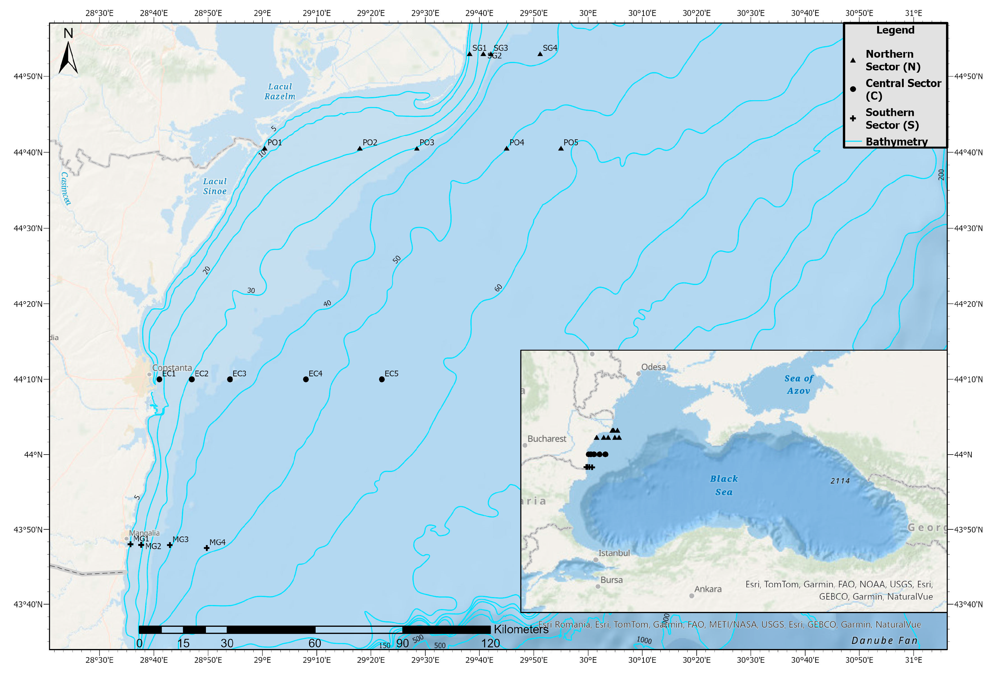
Figure 1. Map of the study area along the Romanian Black Sea coast.
Jmse 14 00730 g001
Figure 2. Principal component analysis (PCA) of the environmental variables recorded along the Romanian Black Sea.
Jmse 14 00730 g002
Figure 3. Box plot of phytoplankton abundance (cells/L) in Black Sea.
Jmse 14 00730 g003
Figure 4. Shade plot with the distribution of phytoplankton according to the density (cells/L) across different stations of the three sectors.
Jmse 14 00730 g004
Figure 5. Box plots of size fractionated ((a). micro-, (b). mezo- and (c). macro-) zooplankton density (ind/m3) across of the three sectors of the Romanian littoral.
Jmse 14 00730 g005
Figure 6. Shade plot showing tintinnid distribution (ind/m3) across stations in the three Black Sea sectors.
Jmse 14 00730 g006
Figure 7. Shade plot illustrating the distribution of mesozooplankton according to the density (ind/m3) across different stations of the three sectors.
Jmse 14 00730 g007
Figure 8. Shade plot illustrating the distribution of macrozooplankton according to the density (ind/m3) across different stations of the three sectors.
Jmse 14 00730 g008
Figure 9. Box plots of ichthyoplankton density (ind/m3) across the three sectors.
Jmse 14 00730 g009
Figure 10. Shade plot illustrating the distribution of ichthyoplankton according to the density (ind/m3) across different stations of the three sectors.
Jmse 14 00730 g010
Figure 11. Box plots of zoobenthos density (ind/m2) across the three sectors.
Jmse 14 00730 g011
Figure 12. Shade plot illustrating the distribution of macrozoobenthos according to the density (ind/m2) across different stations in the three analysed sectors.
Jmse 14 00730 g012
Figure 13. Principal component analysis (PCA) based on scaled environmental and biological variables measured at the Romanian Black Sea. * indicates supplementary variables.
Jmse 14 00730 g013
Figure 14. Fuzzy Cognitive Map (FCM) of trophic interactions. All links represent pairwise correlations between trophic groups. Colours indicate the direction of the relationship (positive or negative), while line thickness reflects the strength of the correlation. Statistically significant interactions (p < 0.05) are highlighted by thicker links.
Jmse 14 00730 g014
Table 1. Physico-chemical parameters analysed in June 2023.
Sector = N
VariableValid NMeanMedianMinimumMaximumLower QuartileUpper QuartileStd.Dev.
T (°C) 921.0821.3219.5322.3220.2321.991.03
S (PSU) 911.8910.846.3418.257.2315.764.85
O2 (µM)9371.42353.71302.79448.83333.16412.6657.05
PO4 [µM] 90.070.050.010.190.010.120.07
SiO4 [µM]9486.59496.20376.50615.60383.50583.20104.38
NO2 [µM]90.360.370.050.840.100.570.29
NO3 [µM]96.242.301.4615.831.789.775.72
NH4 [µM]95.022.861.9013.212.106.983.90
DIN911.629.653.7522.103.8019.268.11
Sector = C
T (°C) 521.0421.0620.3621.6620.9121.190.47
S (PSU)514.7913.1912.8817.5013.1217.282.37
O2 (µM)5346.56358.17314.85377.82322.45359.5126.77
PO4 [µM] 50.120.130.060.180.090.160.05
SiO4 [µM]57.387.406.208.507.207.600.83
NO2 [µM]50.260.250.210.310.240.270.04
NO3 [µM]51.160.950.692.090.881.180.55
NH4 [µM]53.373.411.005.132.544.761.68
DIN54.785.741.946.323.935.981.84
Sector = S
T (°C)420.5220.6119.9420.9320.1320.920.48
S (PSU) 414.2214.1812.5715.9412.5815.861.89
O2 (µM)4374.81373.36359.07393.45364.87384.7514.31
PO4 [µM] 40.010.010.010.010.010.010.00
SiO4 [µM]49.389.606.3012.007.7011.052.38
NO2 [µM]40.100.100.060.150.070.140.04
NO3 [µM]41.751.631.462.291.492.020.38
NH4 [µM]47.246.754.5910.884.7879.703.004
DIN49.098.876.1712.466.7911.392.84
DIN (dissolved inorganic nitrogen) was calculated as the sum of nitrite (NO2), nitrate (NO3), and ammonium (NH4) concentrations (DIN = NO2 + NO3 + NH4).
Table 2. Correlations between biological and environmental factors in each sector analysed.
Sector = N
N = 9 (Casewise deletion of missing data)
VariableT (°C)S (PSU)O2
(µM)
PO4 [µM]SiO4 [µM]NO2
[µM]
NO3
[µM]
NH4
[µM]
DIN
phytoplankton0.544−0.7390.5670.553−0.3780.8730.5060.8570.800
microzooplankton0.099−0.1010.0680.450−0.104−0.0210.232−0.3310.004
mesozooplankton0.749−0.6440.9230.625−0.7060.6910.1170.7890.487
macrozooplankton−0.8390.868−0.853−0.6330.438−0.807−0.608−0.692−0.790
ichtyoplankton0.389−0.3630.1440.554−0.3180.2010.653−0.3030.322
macrozoobenthos0.143−0.3060.256−0.007−0.0200.4310.1410.5970.402
Sector = C
N = 5 (Casewise deletion of missing data)
phytoplankton0.053−0.8210.8680.747−0.6650.392−0.626−0.049−0.224
microzooplankton−0.3980.964−0.886−0.7990.645−0.7010.748−0.292−0.058
mesozooplankton0.422−0.9280.7840.776−0.4010.926−0.5380.5770.386
macrozooplankton
ichthyoplankton
macrozoobenthos−0.1310.2240.0730.046−0.477−0.641−0.163−0.995−0.973
Sector = S
N = 4 (Casewise deletion of missing data)
phytoplankton0.929−0.9740.655−0.886−0.103−0.4750.9950.987
microzooplankton0.565−0.501−0.120−0.6580.607−0.1500.7370.768
mesozooplankton0.603−0.7610.993−0.557−0.811−0.5850.5660.508
macrozooplankton−0.8260.953−0.8850.8460.4940.646−0.881−0.838
ichthyoplankton0.443−0.5040.001−0.8460.315−0.5360.7550.731
macrozoobenthos−0.1400.002−0.305−0.5860.208−0.6240.2880.224
Table 3. Correlations between trophic components’ abundances.
VariablePhytoplanktonMicrozooplanktonMesozooplanktonMacrozooplanktonIchthyoplanktonMacrozoobenthos
phytoplankton
microzooplankton−0.218
mesozooplankton0.514−0.221
macrozooplankton−0.443−0.340−0.570
ichthyoplankton0.1350.0540.155−0.121
macrozoobenthos0.4480.077−0.084−0.2030.402
Table 4. Structural indices of the Fuzzy Cognitive Map (FCM), including indegree, outdegree, centrality, and functional role of each trophic component.
ComponentIndegreeOutdegreeCentralityType
Phytoplankton01.161.16Driver
Microzooplankton0.210.320.53Ordinary
Mesozooplankton0.730.671.4Ordinary
Macrozooplankton0.570.320.89Ordinary
Ichthyoplankton0.120.40.52Ordinary
Macrozoobenthos1.2401.24Receiver
Table 5. Pearson and partial correlations for key trophic interactions in the Black Sea.
InteractionPearson Correlation (r)Correlation with
Controlling Variable
Controlling Variable (Z)Partial Correlation
Phytoplankton–Mesozooplankton+0.514phyto–NH4: +0.641NH4+0.255
meso–NH4: +0.546
Macrozooplankton–Mesozooplankton–0.570macro–S: +0.491Salinity (S)–0.501
meso–S: –0.315
Disclaimer/Publisher’s Note: The statements, opinions and data contained in all publications are solely those of the individual author(s) and contributor(s) and not of MDPI and/or the editor(s). MDPI and/or the editor(s) disclaim responsibility for any injury to people or property resulting from any ideas, methods, instructions or products referred to in the content.