Article

Impact of the Surface Roughness of Artificial Oyster Reefs on the Biofouling and Flow Characteristics Based on 3D Scanning Method


Department of Marine Fisheries, Fisheries College, Ocean University of China, Qingdao 266003, China
*
Author to whom correspondence should be addressed.
J. Mar. Sci. Eng. 2026, 14(8), 703; https://doi.org/10.3390/jmse14080703
Submission received: 2 March 2026 / Revised: 26 March 2026 / Accepted: 4 April 2026 / Published: 10 April 2026
(This article belongs to the Section Marine Aquaculture)

Abstract

The complex surface architecture of natural oyster reefs is widely considered to promote biological attachment, yet the underlying mechanisms and the relevance to the design of artificial reefs are not fully understood. Here, we combined field experiments, 3D surface characterization, and numerical modelling to quantify how reef-like roughness regulates biofouling development and near-wall flow around artificial substrates. Surface morphological characteristics of natural oyster reefs were first obtained by 3D scanning and used to fabricate concrete panels with simulated rough textures, while traditional smooth concrete panels served as controls. The two types of panels were simultaneously deployed in the target sea area for a hanging-panel experiment. Samples were collected after 3, 6, 9, and 12 months to track changes in biofouling communities. At each sampling time, the panel surfaces were quantified by canopy roughness ( R C ), surface heterogeneity ( σ ), and fractal dimension ( D ), and these metrics were integrated into numerical simulations combined to resolve the flow field, turbulence kinetic, and near-wall shear stress around the colonized panels. The research results show that, after 12-month immersion, the mean thickness of the biofouling layer on rough and control panels reached 6.39 mm and 5.91 mm, respectively. Rough panels exhibited consistently higher R C and σ than controls, and these two parameters are strongly linearly correlated ( R 2 = 0.891 ) . Numerical simulations reveal that increased R C enlarges the oyster settlement shear-stress window (OSSW), indicating more favorable hydrodynamic conditions for oyster settlement and growth on rough panels. Nevertheless, the hydrodynamic differences between the initial rough panels and control panels gradually diminish over time, suggesting that biological growth can progressively naturalize initially smooth substrates. These findings advance the mechanistic understanding of how small-scale roughness and biofouling co-evolve to shape oyster habitat quality and provide a quantitative basis for the eco-engineering design of artificial oyster reefs.

1. Introduction

Artificial reefs are widely used in coastal and marine environments as engineered structures designed to enhance ecological functions, support fisheries, and provide shoreline protection [1,2]. Across different regions worldwide, artificial reefs have been constructed using a variety of materials and configurations, ranging from purpose-built modules to repurposed infrastructure, with applications spanning habitat restoration, biodiversity enhancement, and coastal defense [3]. Among the various types of artificial reefs, oyster reefs have attracted particular attention due to their strong ecological functionality and their ability to modify local hydrodynamic conditions [4]. By filtering suspended organic particles and plankton, oyster assemblages effectively improve water quality [5], reduce eutrophication pressure, and help immobilize contaminants [6]. Their complex three-dimensional structures also modify near-bed hydrodynamics, attenuate wave and current energy, and enhance sediment trapping and bed stabilization [7,8,9]. Together, these functions create heterogeneous microhabitats that function as high-quality spawning, nursery, and refuge areas for diverse taxa, underpinning biodiversity and playing a pivotal role in the conservation and recovery of fisheries resources [10,11]. However, due to overfishing, pollution, and habitat degradation, natural oyster reefs have declined dramatically [12], with an estimated 85% lost or severely degraded worldwide [13,14].
In response, artificial reefs have been widely deployed to support habitat restoration and coastal management [15,16,17]. A variety of artificial materials and structures have been deployed to facilitate reef restoration, including the placement of loose shell, concrete rubble, prefabricated reef modules, and panel-based systems around the world [18]. Among these, concrete and other hard substrates are widely used due to their durability, low cost, and suitability for large-scale applications. Increasing evidence shows that surface morphology and roughness of such structures strongly influence larval settlement [19], early biofouling, and near-bed hydrodynamics, thereby affecting community development and ecological performance [20,21]. However, despite this recognition, systematic research that quantitatively links controllable engineering attributes (e.g., surface texture metrics) to ecological outcomes (e.g., colonization rates, biomass accumulation, and community composition) is still lacking. Existing studies are largely descriptive or comparative and seldom produce transferable, predictive relationships that can be directly applied to engineering design [22,23]. Consequently, practical reef and coastal infrastructure construction remains largely empirical, and many installations still rely on simple flat or coarsely textured concrete elements, lacking ecology-informed guidelines for configuring surface features to promote desired ecological functions [24,25]. Addressing this gap requires a more mechanistic understanding of how engineered surface characteristics influence physical processes and, ultimately, ecological performance. In recent studies, Levy et al. (2022) used 3D methods to capture reef geometry and biodiversity, offering promising tools for detailed characterization, but the critical step of turning such geometric descriptors into quantitative, design predictors of ecological function remains an important knowledge gap [26].
The microtopography of reef surfaces, including roughness, height variability, and the presence of pores and crevices, has been shown to strongly affect larval settlement, attachment success, and subsequent community succession [27,28]. Roughened or structurally complex substrates can also modify near-bed flow velocities, shear stress, and local vortex structures, thereby influencing the transport and deposition of nutrients, suspended particles, and larvae [29,30]. Importantly, higher flow and turbulence may increase larval delivery to the bed, yet can simultaneously reduce anchoring probability and increase post-contact detachment. Thus, overall settlement success often depends on whether larvae can encounter sheltered, low-shear microhabitats within the reef matrix [31,32,33]. Accordingly, some studies have used quantitative descriptions such as fractal dimension, surface heterogeneity indices, and roughness parameters to characterize the surface complexity of natural oyster reefs [34], and CFD-based (Computational Fluid Dynamics) simulations have been employed to explore how different roughness configurations affect local flow fields and vorticity patterns [35]. Hydrodynamic conditions, particularly flow speed and direction, are known to be critical for oyster larvae during the settlement phase [29]. Because their swimming ability is weak and larvae are largely transported passively in the water column, excessive near-bed flow velocities can hinder their ability to attach and metamorphose on hard substrates, whereas structurally complex surfaces may create refugia that locally attenuate shear and extend the time window for exploration and attachment between stress pulses [31,33].
Recent studies have shown that oyster reef surface roughness and morphological complexity can strongly modify local hydrodynamic conditions, but current understanding remains derived largely from rough-wall flow theory, experimental observation, and idealized representations of reef surfaces. Field and flume observations have shown that reef-scale roughness can increase drag and turbulence above the canopy while creating low-velocity, low-shear refugia within interstitial spaces, thereby enhancing larval recruitment and attachment success [29]. However, observations and experiments alone cannot fully resolve the fine-scale mechanisms governing near-surface velocity gradients, vortex development, and particle retention, which motivates the use of CFD for mechanistic analysis. More recently, LBM-LES (Lattice Boltzmann Method and Large Eddy Simulation) studies showed that gaps and branching structures associated with different reef growth stages can generate complex turbulence and irregular vortex shedding [35]. Substrate-design study combining PIV (Particle Image Velocimetry) and CFD demonstrated that engineered micro- and meso-scale surface features can alter near-bed hydrodynamic conditions and enhance particle retention [36]. However, these numerical studies still rely on simplified shell morphologies, smooth surface assumptions or bulk empirical metrics such as rugosity and surface area ratio, and they are commonly restricted to unidirectional steady inflow. As a result, little is known about how reef- or panel-scale roughness evolves with biofouling and how this bio-induced morphological change feeds back on local hydrodynamics, particularly near-surface flow and vortex structures over time.
Motivated by Temmink’s (2023) emergent trait (mimicry concept) [37], this study adopts a biomimetic and process-based approach to investigate how naturally developed surface textures modify the local physical environment of artificial oyster reef substrates. By combining offshore panel deployment, biofouling monitoring, high-resolution 3D scanning, and three-dimensional numerical simulations, we compare biomimetic and conventional concrete oyster-reef panels in terms of biofouling development, the resulting evolution of surface roughness, and the associated changes in local hydrodynamics responses. Here, we hypothesize that: (i) increasing surface roughness enhances flow heterogeneity and turbulence intensity near the substrate, thereby creating more favorable microhabitats for oyster larval settlement; (ii) different roughness configurations generate distinct flow structures, leading to measurable differences in flow retention, shear stress distribution, and near-bed velocity; (iii) there is an optimal range of roughness that balances hydrodynamic stability and ecological functionality, rather than a simple monotonic relationship. This study focuses on panel-scale responses during the first year of deployment at a single field site. It emphasizes temporal changes in biofouling accumulation and surface roughness. Computational fluid dynamics (CFD) was used to resolve first-order flow–roughness interactions under representative steady inflow conditions. The results should therefore be interpreted as a mechanistic and design-oriented assessment at the panel scale, rather than as a complete representation of reef-scale hydrodynamics across all environmental settings.

2. Materials and Methods

2.1. Study Area and Panels Deployment Setup

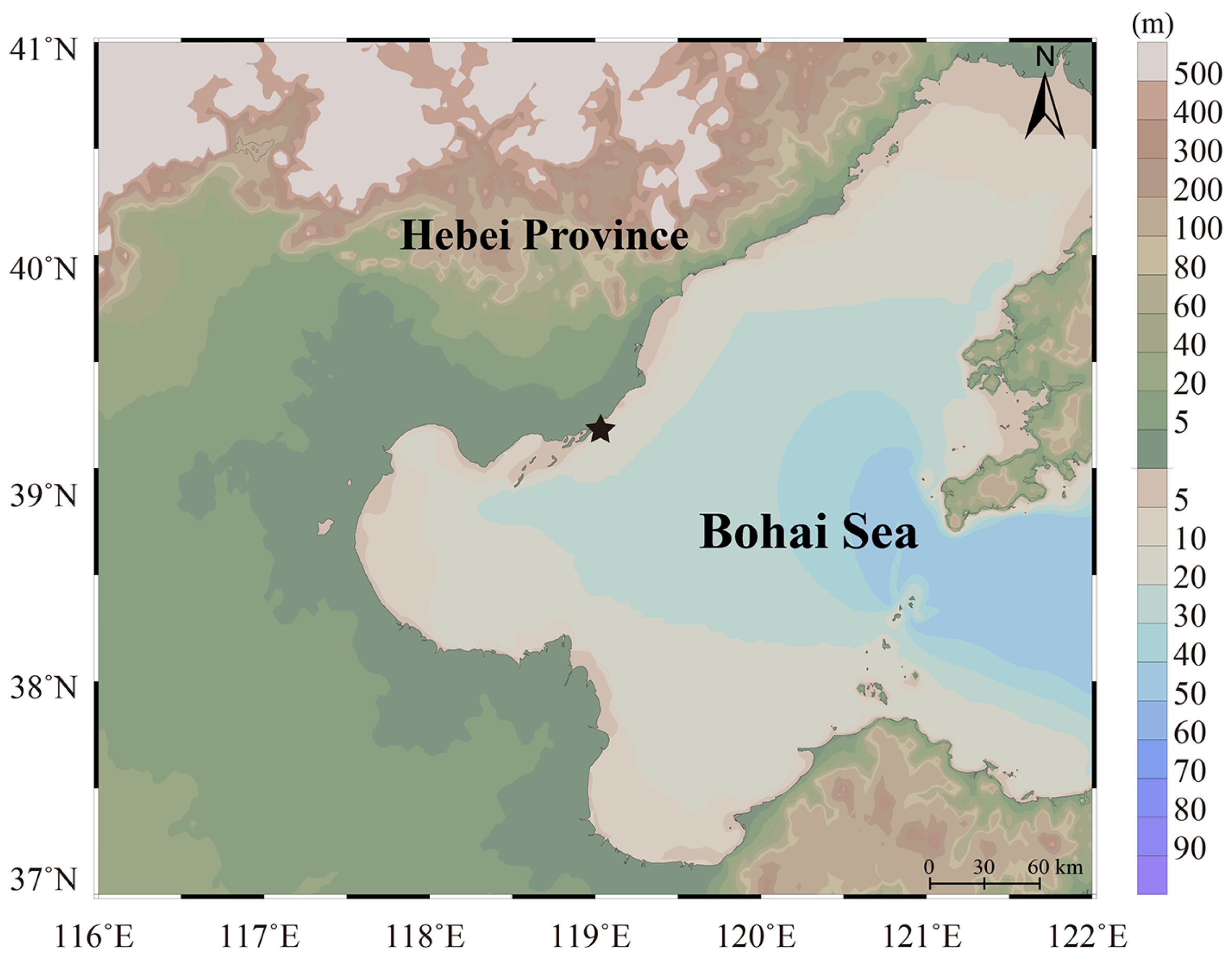
The study area is located in Xiangyun Bay, Bohai Sea, China (39°10′ N, 119°00′ E) (Figure 1). It lies within the circulation zone at the mouth of the Luan River Estuary and is characterized by a humid continental monsoon climate with four distinct seasons and coincident peaks of rainfall and temperature. This area provides stable tidal and current conditions, a flat muddy-sandy seabed, and the advantage of historical oyster reef resources [18,38], making it highly suitable for panel-based mariculture.
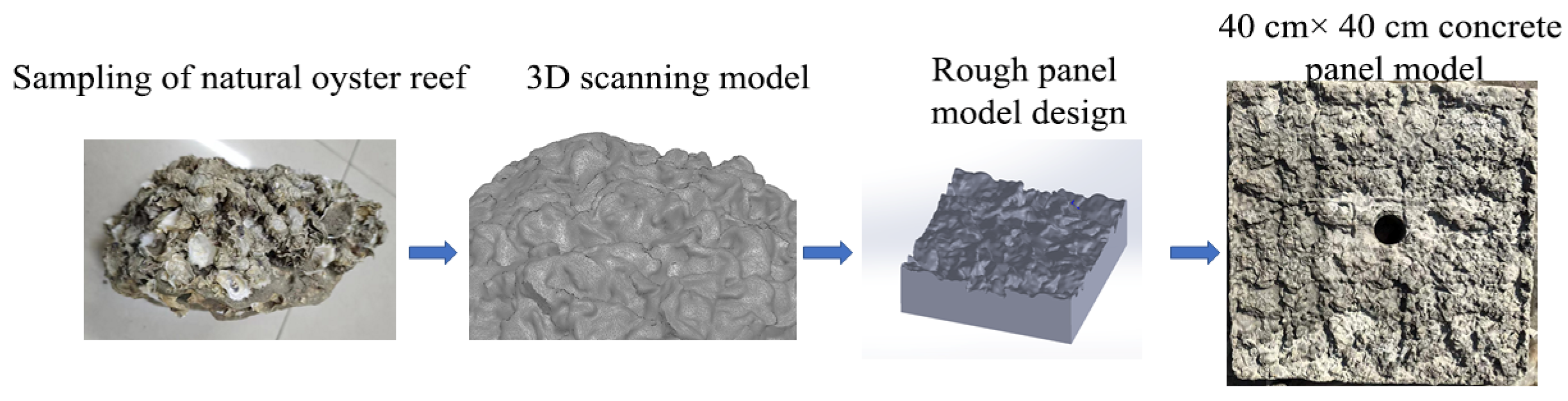
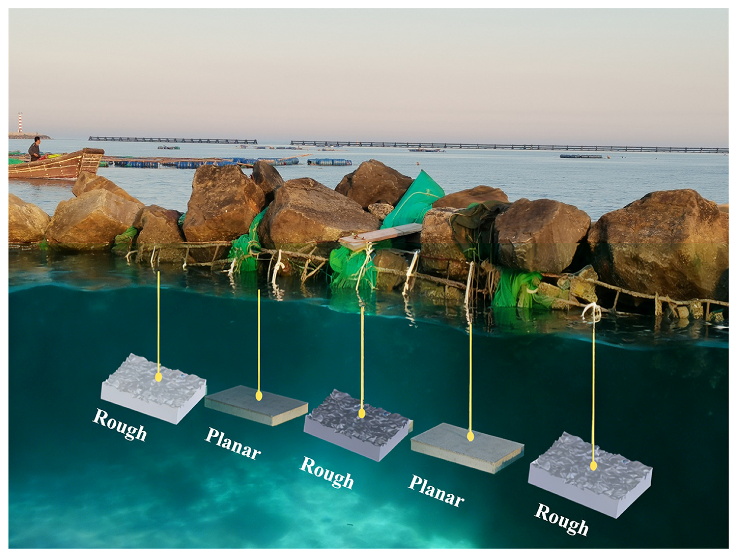
In this study, concrete settlement panels with dimensions of 40 cm × 40 cm were used. The experimental panels were designed on the basis of three-dimensional scanning data of natural biogenic reef structures in Xiangyun Bay, in order to reproduce their complex surface topography (Figure 2). Panels of the same size but with a smooth, planar surface were fabricated as the control group. A total of 30 panels of each type were deployed. As shown in Figure 3, the panels were installed in nearshore waters adjacent to a breakwater within the study area. They were suspended from a horizontal support line fixed to the crest of the breakwater, using a system of vertical drop lines. This configuration allowed the panels to remain relatively stable in the water column with uniform spacing, thereby reducing mutual shading and minimizing localized flow disturbance effects. To reduce potential systematic bias arising from spatial position, experimental and control panels were arranged alternately along the same support line, ensuring that both panel types experienced comparable hydrodynamic conditions. All panels were suspended within the same depth range (e.g., 4 m from the water surface), and their upper edges moved coherently, a disturbance characteristic of shallow coastal environments. The study site was selected primarily based on its suitable water depth for panel deployment and its potential to support oyster larval recruitment, thereby ensuring the feasibility of the field experiment.
To ensure that the textured surface of the experimental panels consistently faced upstream and toward the open water, and to avoid contact with seabed sediments due to panel tilting or flipping, divers inspected and adjusted the orientation and hanging posture of each experimental panel individually. This procedure helped to maintain consistent and reliable experimental conditions through the deployment period.
The hanging-panel experiments began in June 2024. Panels were recovered after 3, 6, 9, and 12 months, and at each sampling time, three experimental panels and three control panels were randomly selected for analysis. To quantify changes in canopy roughness induced by biofouling over time, three-dimensional scans of the panel surfaces were acquired before deployment and at each subsequent recovery time (3, 6, 9, and 12 months). Before scanning, only the biofouling attached to the mounting interfaces was gently removed to stabilize the scanning posture, while the fouled surface itself remained intact. Each panel was mounted on a custom stand with a height of 21 mm, positioning the fouled surface parallel to the smooth reference plane beneath it and preventing tilt induced by organisms growing on the non-scanned side.

2.2. Surface Roughness Calculation Based on 3D Scanning

2.2.1. Point-Cloud Data Processing of 3D Scanning Model

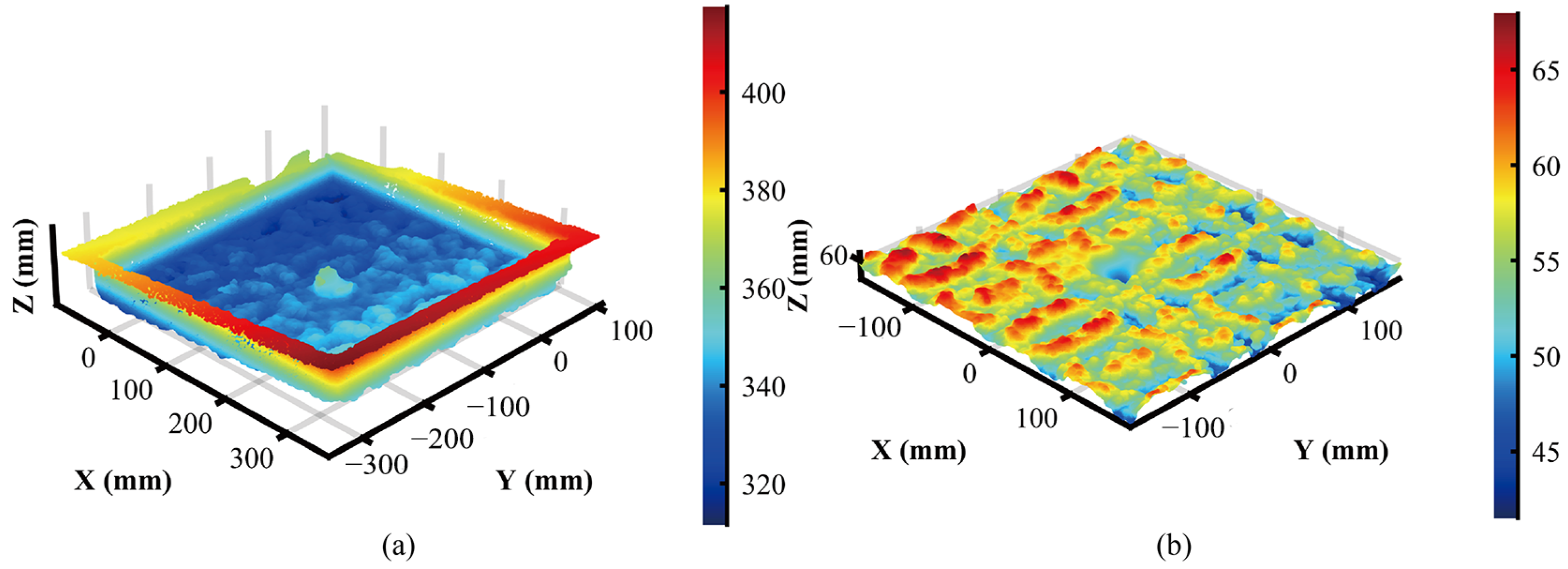
Point-cloud processing was conducted in Geomagic Wrap 2021. The analysis area was first trimmed to a 34 cm × 34 cm square corresponding to the central settlement surface, thereby excluding edge and side-wall fouling from subsequent calculations. Isolated external points and non-connected elements were removed to reduce noise associated with repeated scans. Remaining voids in the central region of the panels were then reconstructed using a curvature-based hole-filling algorithm. To establish a consistent spatial reference frame across all samples, the reference plane was translated upward by 21 mm and defined as the XY plane, and the YZ plane and XZ planes were adjusted using the software’s symmetry tools to align panel orientation among scans, as shown in Figure 4. The final surface models retained for analysis had point-cloud densities exceeding 1,000,000 pts/m2, ensuring sufficient spatial resolution for subsequent roughness characterization.

2.2.2. Roughness Indices of the Panel with Biofouling

In this study, to quantitatively characterize the roughened surfaces generated by different fouling communities on the panels, we computed a suite of key roughness metrics, including biofouling thickness ( H ), canopy roughness ( R C ), local surface slope ( S ), surface heterogeneity ( σ ), and fractal dimension ( D ). Biofouling thickness ( H ) was used to characterize the overall elevation of the fouling canopy. Let Z(x,y) denote the pre-process elevation of the point cloud. The biofouling thickness H and biofouling thickness increment H were calculated as
H t , j = 1 N i = 1 N Z i H 0 , H t = 1 3 j = 1 3 H t , j 1 3 j = 1 3 H t t , j
where N is the number of the valid points; Z i is the elevation of point i ; H 0 is the mean elevation of the original, unfouled panel surface; j denotes the replicate specimen among three parallel panels sampled at each time ( j = 1 ,   2 ,   3 ) , t is the sampling time, t is the time interval.
To quantify the geometric roughness of the fouling canopy, we adopted a “canopy roughness” index R C , analogous in form to traditional rugosity measures used in coral-reef ecology but adapted to the microtopography of fouled panels. Rugosity was defined as the ratio between the three-dimensional surface area of the fouling canopy and its planar projection area:
R C = A 3 D / A 2 D
where A 3 D is the total area of the reconstructed 3-D canopy surface and A 2 D is the orthogonal projection area of the same region onto the basal plane. The projection area A 2 D was fixed at 115,600 mm2, corresponding to the 34 cm × 34 cm analysis window.
The 3-D canopy area A 3 D was obtained via a high-fidelity surface-reconstruction workflow. First, processed point clouds were converted into continuous triangle-mesh surfaces in Geomagic Wrap, effectively performing linear interpolation between points to generate a smooth, gap-free digital surface model. Second, the mesh was imported into SpaceClaim (Ansys SpaceClaim 2025 R2), which was used to compute the total area of the irregular surface. This approach preserves the high spatial resolution of the original scans while avoiding excessive sensitivity to very small-scale roughness, producing a “virtual sheet” draped over the fouling canopy. Conceptually, it is analogous to the classical chain-and-tape method, extracting roughness at the dominant structural scale and yielding values comparable to traditional ecological rugosity metrics, but with the added precision and efficiency of 3D techniques.
The overall roughness slope is characterized by its areal mean and RMS values, consistent with standard 3D surface texture parameters and similar to the “effective slope” measures used in rough-wall turbulence studies [39,40,41,42]. The local surface slope was quantified as the magnitude of the height gradient:
S ( x , y ) = z x 2 + z y 2
where z / x and z / y are the local slope components in the streamwise and spanwise direction, respectively.
z x i , j z i + 1 , j z i 1 , j 2 x , z y i , j z i , j + 1 z i , j 1 2 y
S i , j = z x i , j 2 + z y i , j 2
The mean and root-mean-square (RMS) value over the entire measurement area is used as follows:
S ¯ = i , j S i , j N ( i , j ) , S R M S = i , j S i , j 2 N i , j
Surface heterogeneity ( σ ) was used to describe the spatial dispersion of elevation values, reflecting the intensity of microtopographic relief. It was defined as the standard deviation of all cell elevations within the analysis window:
σ = 1 N 1 i = 1 N ( Z i H ) 2
Large values σ indicate more dispersed elevation distributions and stronger local relief. In contrast to canopy roughness R C , which emphasizes the overall geometric complexity of the surface, σ focuses on local variations in height. All computations were performed in Python 3.10 using the numpy mean () and std () functions. As above, elevation data were analyzed within a fixed 34 cm × 34 cm window, with coordinates expressed in millimeters to maintain consistency among samples.
Building on these metrics of biofouling thickness, rugosity, and local elevation variability, we further quantified the scale-dependent complexity of the fouled surfaces using a fractal dimension D . The fractal dimension D , was estimated with the variation method, which relates elevation variability to observation scale and is well suited for noisy, naturally fouled surfaces. Let the gridded surface be represented by Z ( x , y ) . For a given window size ε , the surface is partitioned into square windows of ε × ε , and the heights within each window are computed as
v i j ε = max Z i j m i n Z i j
The mean variation at scale ε is then
V ε = 1 N ( ε ) i j v i j ε
where N ( ε ) is the number of the square windows. For a surface with fractal properties, a power-law relationship with scale,
V ( ε ) ε 3 D
which leads to a linear relationship in log-log space:
log V ε = 3 D log ε + C
We projected the point clouds onto a regular height grid with a cell size of 1 mm, ensuring consistent units in all three directions (x, y, z in mm). For each panel, V ( ε ) was calculated for window sizes ε = 2 ,   4 ,   8 ,   16 ,   32 ,   64   m m , and log   V ( ε ) was regressed against log ε using ordinary least squares. The regression slope k of this relationship was used to derive the fractal dimension as D = 3 k .
Only fits with R 2 0.90 were retained. All calculations were performed in Python using numpy and scipy.stats. For a perfectly smooth plane, D 2 ; increasing canopy roughness and greater coverage by organisms such as oysters lead to higher D values, indicating more complex and structurally rough surfaces.

3. Numerical Simulation Method Based on CFD

3.1. Numerical Model of the Fouled Panels

To illustrate how panel surface morphology influences biofouling through near-bed hydrodynamics, all experimental panels were subjected to flow-field simulations using ANSYS Fluent 2025 R2. The pre-fouling controlled panel was represented as a rectangular block with dimensions 34 cm × 34 cm × 5 cm. Rough panels were constructed from the corresponding surface point-cloud data: processed meshes from Geomagic Wrap were converted to closed triangular surfaces and automatically surfaced, and the resulting solid models were exported as STP files for import into Fluent. Fluent solves the governing equations using the finite-volume method, which provides flexible mesh generation, good adaptability to complex geometries, and strict conservation of mass and momentum. This makes it suitable for resolving detailed wake structures and near-wall flows around artificial reefs, like bodies such as the rough fouled panels considered here.

3.2. Governing Equations and Turbulence Model

The flow was assumed to be incompressible and Newtonian. In a three-dimensional Cartesian coordinate system, the Reynolds-averaged continuity and momentum equations are
u ¯ i x i = 0
u j ¯ u i ¯ x j = f ¯ i 1 ρ p ¯ x i + 1 ρ μ 2 u ¯ i x j x j ρ u j u i ¯ x j
where ρ is the flow density; u ¯ i is the time-averaged velocity vector ( i = 1 ,   2 ,   3 ) for x ,   y ,   a n d   z , respectively; p ¯ is the static pressure; x i   represents the spatial coordinate; u i and u j represent the fluctuating velocity ( i ,   j = 1 ,   2 ,   3 ), respectively; ρ u j u i ¯ is the Reynolds stress due to the fluctuating velocity field; f ¯ i   is any additional body forces ( i = 1 ,   2 ,   3 ); ν = μ / ρ is the kinematic viscosity; μ is the dynamic viscosity.
In this paper, the turbulence closure is provided by the k ω shear-stress-transport (SST) model, which blends the near-wall performance of the standard k ω model with the robustness of the k ε formulation in the outer flow via a set of blending functions. The transport equations for turbulent kinetic energy   k and specific dissipation rate ω are
The turbulence kinetic energy ( k ) by [43]:
ρ k t + ρ u j k x j = x j μ + σ k μ t k x j + P k β * ρ ω k
The specific turbulence dissipation rate ( ω ) equation is given by:
( ρ ω ) t + ( ρ u j ω ) x j = x j [ ( μ + σ ω μ t ) ω x j ] + α ω k P k β ρ ω 2 + 2 ( 1 F 1 ) ρ ω σ ω 2 k x i ω x i
where u j is the time-averaged velocity component in direction j ; μ t   is the turbulent dynamic viscosity; σ k ,   σ ω , σ ω 2 are model constants acting as the turbulent Prandtl numbers, representing diffusive transport of k and ω , respectively; The source term P k   is the production of turbulence kinetic energy; β * is constant in the S S T k ω formulation, 0.09; α is a constant associated with the production of ω ; β is a model constant associated with the destruction of ω ; F 1 is the blending function of the S S T   k ω model, which controls the transition between the near-wall k ω region and the outer-flow k ε region.

3.3. Computational Domain and Meshing Method

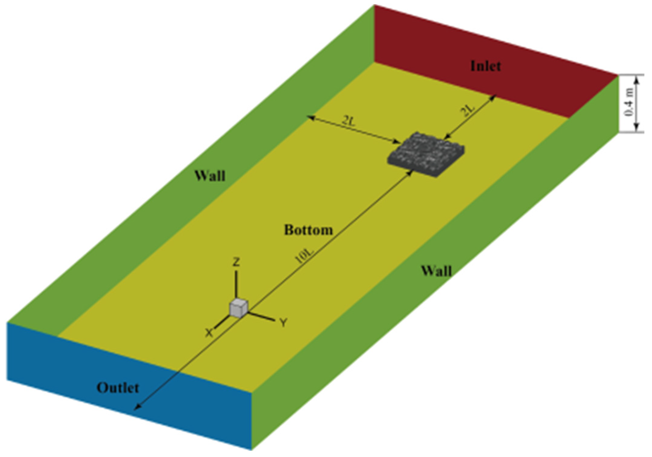
As shown in Figure 5, the size of the computational domain was designed according to the characteristic length L of the panel. The inlet and lateral walls were placed 2   L upstream and sideways from the panel, the outlet was located 10   L downstream, and the top boundary was positioned at a height of L above the panel. To improve the accuracy of the simulation, a locally refined sub-domain was embedded around the panel: the upstream, lateral, and upper faces of the refinement region were placed 0.5   L from the panel, and its downstream face was located 2   L downstream.
Boundary conditions were specified as follows:
(1)
Inlet: a velocity inlet with a uniform inflow speed of 0.5 m·s−1  ( u 0 = 0.5   m / s ) . Because the present simulations were conducted under steady-state conditions, a single representative inlet velocity was prescribed. The value of 0.5 m/s was selected as an intermediate typical flow velocity in Xiangyun Bay, representing a moderate hydrodynamic condition. Turbulent kinetic energy k and specific dissipation rate ω at the inlet were prescribed from standard turbulent relations.
(2)
Outlet: a pressure-outlet condition, allowing the flow to leave the domain without artificial reflection.
(3)
Walls: the domain bottom and all panel surfaces were treated as smooth no-slip walls, enforcing zero fluid velocity at the wall;
(4)
Top and side boundaries: the top boundary and the vertical side walls of the outer domain were specified as symmetry planes, implying zero normal velocity and zero normal gradients of tangential velocities.
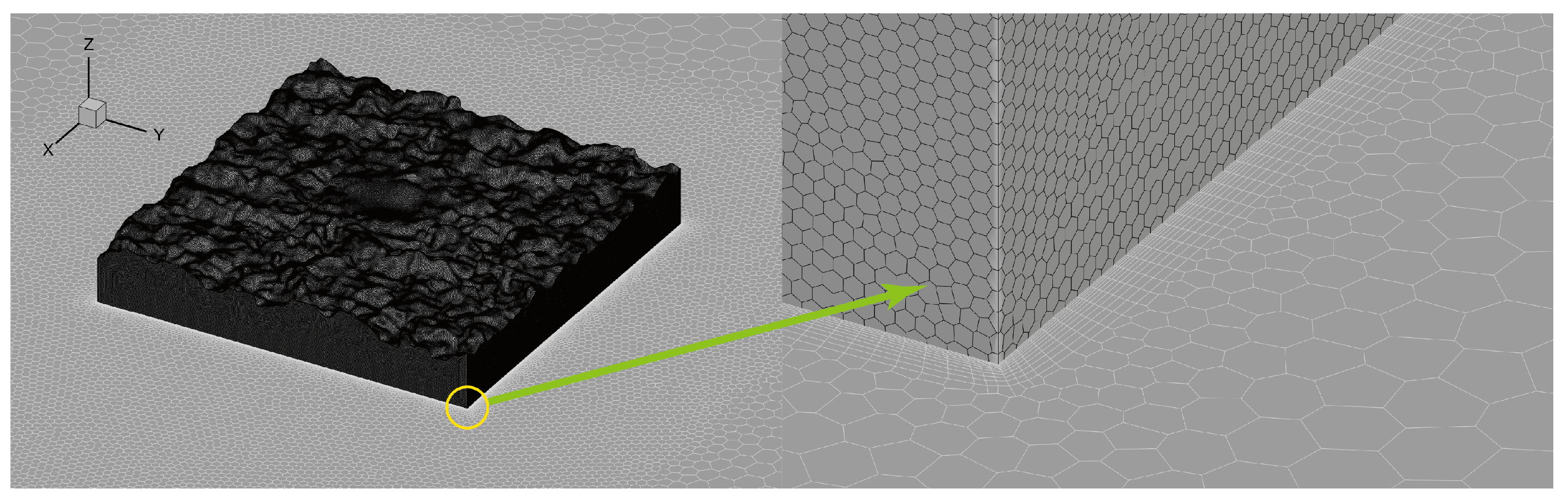
In the flow simulations, the computational mesh was generated in Fluent Meshing using the poly-hexcore technique. Figure 6 shows the mesh generation of the computational domain adopted in this study. The fluid domain around the biofouled panel was discretized with a Cartesian hexcore in the outer region and body-fitted polygonal cells in the vicinity of the solid boundaries. Near the panel and bottom surface, several layers of highly stretched cells were inserted in the wall-normal direction to resolve the strong velocity gradients and wall shear stress. Local grid refinement was applied around the panel edges and corners so that the complex biofouled topography and the associated separation and reattachment zones could be adequately captured. The final mesh contains approximately 5.4~5.8 million cells. The surface mesh is controlled with a minimum element size of 0.85 mm and a maximum size of 34 mm, and a growth rate of 1.2. A Curvature and Proximity size function with a curvature normal angle of 18° and at least three cells per gap is employed, with proximity applied to both faces and edges. These settings ensure sufficient resolution of the small-scale roughness features on the biofouled panel while keeping the overall cell count at a tractable level. Because the S S T   k ω turbulence model is used, the near-wall spacing was chosen such that the non-dimensional wall distance on the biofouled panel surfaces satisfies y + 1 over most of the area. This configuration allows the viscous sublayer to be directly resolved without resorting to wall functions, and provides a reasonable compromise between numerical accuracy and computational efficiency for resolving the near-panel flow. Details of the mesh independence test and turbulence model validation against PIV measurements are provided in Appendix A.

3.4. Flow Characteristic Indices Around the Biofouling Panels

To compare and quantify the flow characteristics induced by biofouling panels with different levels of biofouling, we introduce several flow characteristic indices around the panel, including the relative velocity, the upwelling volume, the wake volume, the vortex, and the wall shear stress. The upwelling region is defined as the set of grid cells where the vertical velocity exceeds a fixed fraction of the incoming velocity, u z > 0.1 u 0 . The wake region is identified as the set of cells with flow reversal in the streamwise direction, u x < 0 . These quantities are defined below and are used to relate the evolution of the biofouling roughness geometry to the modification of the local flow field and turbulence.
To obtain measures that are independent of the absolute panel size, the volumes are normalized by the panel volume V p a n e l [44]:
I u p = V u p w e l l i n g V p a n e l ,   I w = V w a k e V p a n e l
where u 0 is the undisturbed incoming velocity, 0.5 m/s; u x and u z are the horizontal and vertical velocity components, respectively. V u p w e l l i n g   and V w a k e are the volumes of the upwelling and wake region around the panel, respectively; V p a n e l is the volume of the biofouling panel, varying with immersion time.
To characterize the strength of the vortical motion induced by the panel, we compute a vortex index based on the spatially averaged vorticity components [45]:
ω y = u i z w i x ,   ω z = v i x u i y
where u i ,   v i ,   w i is the velocity components at grid point i , and N   is the number of grid points in the region of interest. The z-direction represents the vertical direction, the x–y plane is the horizontal plane, and the origin is located at the center of the bottom base of the panel. These average vorticity components provide a compact measure of the intensity of streamwise and spanwise vortices around the panel, and are later used to compare the flow response to panels with different biofouling stages.

4. Results

4.1. Temporal Dynamics of Biofouling Thickness ( H ) and Biomass

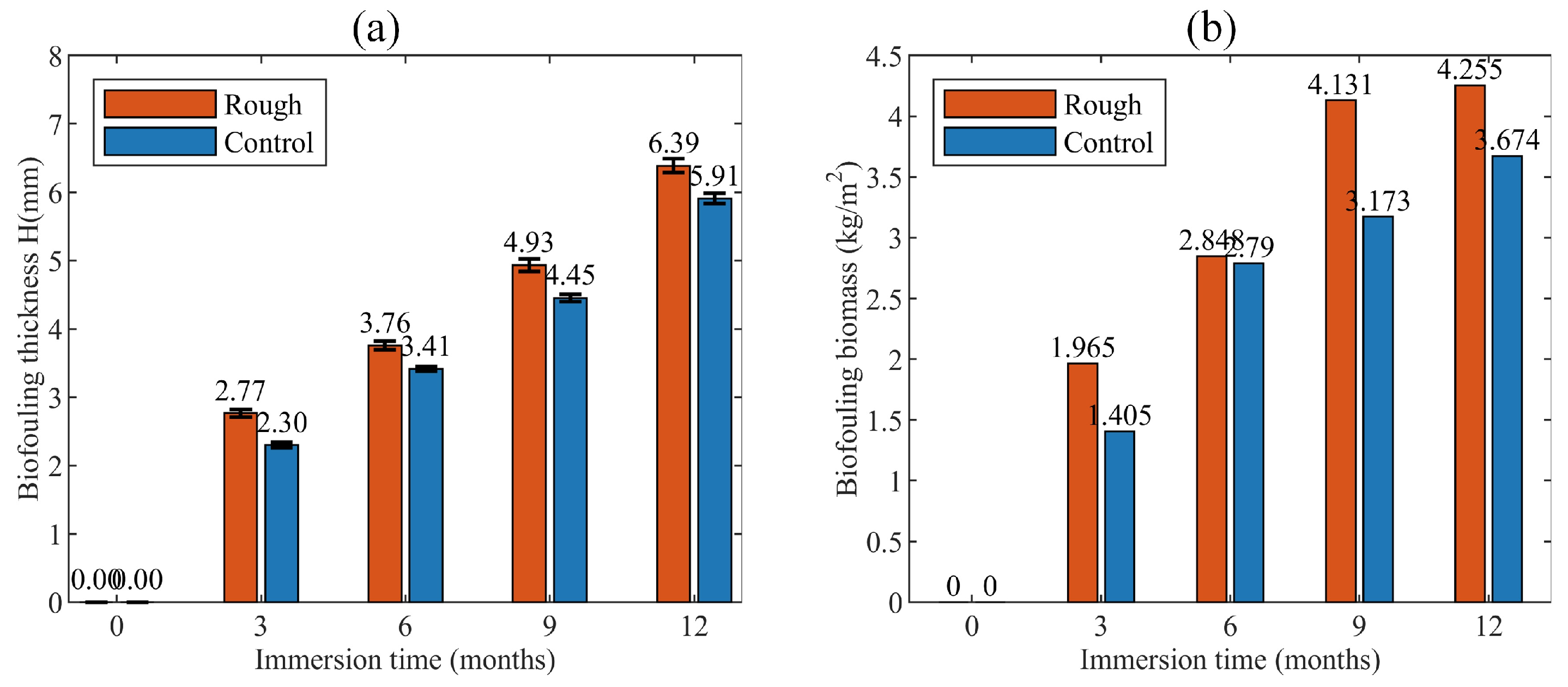
Figure 7 presents the variation of H and the biomass of the experimental and control panels throughout one year of immersion. Over the 12-month experiment, both H and biomass on the roughened panels increased steadily, and two-way ANOVA showed that panel type and time had significant interactive effects on both variables ( p < 0.001 ) . At 3 months, the biofouling thickness on rough panels already exceeded that on control panels, see Figure 7a. Thereafter, the biofouling thickness on rough panels increased rapidly and remained consistently higher than on control panels throughout the experiment (Table 1). Here, H indicates the biofilm thickness increase during each sampling interval. By 12 months, rough panels reached a mean biofouling thickness of 6.39 ± (0.10) mm, compared with 5.91 ± (0.07) mm on control panels, corresponding to an increase of approximately 8.12%. Differences between panel types were significant at each sampling time ( p < 0.05 ). Biofilm biomass showed a similar but more pronounced pattern (Figure 7b). Initial biomass on rough panels was modestly higher than on the control panels; however, from 3 months onward, rough panels accumulated biomass much more rapidly. After 12 months, biomass on rough panels reached 4.255 kg·m−2, nearly 15% greater than on the control panel. Repeated-measures ANOVA confirmed significant main effects of panel type and time, as well as a significant interaction ( p < 0.001 ), indicating that roughness modified the temporal trajectory of biomass accumulation rather than simply shifting absolute values.
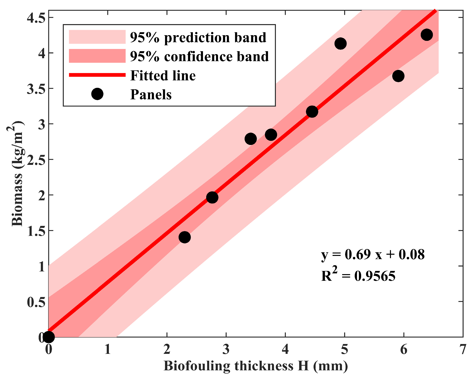
Across all panels and sampling times, biofouling thickness and biomass were strongly and positively correlated (Figure 8). Pearson correlation analysis yielded r   = 0.934 ( p < 0.001 ), indicating that increasing biofouling thickness was closely associated with increasing standing stock of attached organisms. Linear regression further showed that biomass could be reliably estimated from biofouling thickness:
y = 0.69 x + 0.082
where x is the mean biofouling thickness (mm) and   y is biomass (kg·m−2). The narrow 95% confidence band around the fitted line (Figure 8) suggests limited scatter and supports the use of biofouling thickness as a robust proxy for biofouling biomass at the panel scale.

4.2. Temporal Evolution of Surface-Morphology Parameters

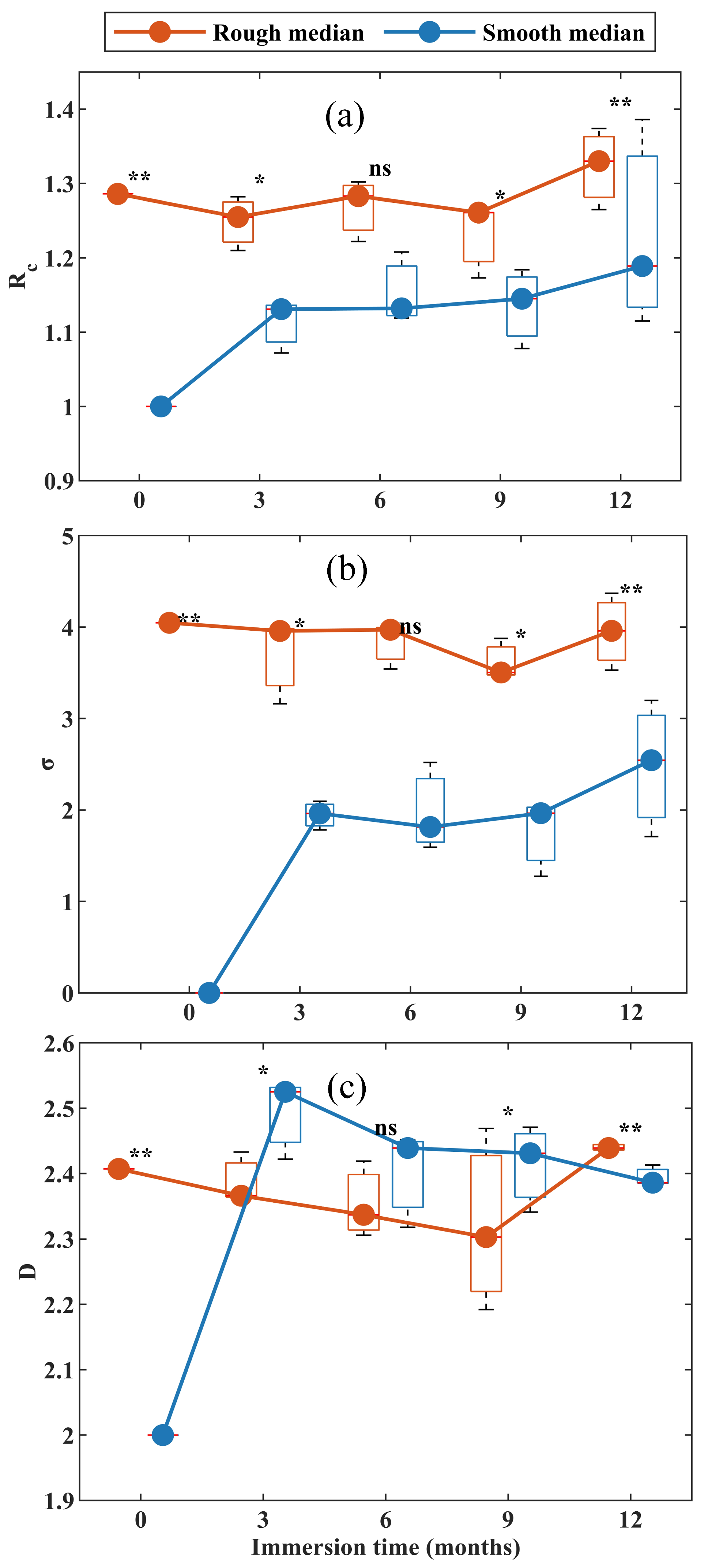
To illustrate the mechanisms underlying differences in biofouling thickness ( H ), we quantified the temporal evolution of three key descriptors of microtopography: canopy roughness R C , surface heterogeneity σ , and fractal dimension D . Figure 9 shows that biological colonization progressively increased the canopy roughness and height variability of the control panels, whereas the pre-existing differences between the rough and control panels were not fully eliminated over the 12 months. At deployment (0 months), rough panels exhibited much larger R C , σ , and slightly higher D than control panels, reflecting the deliberately manufactured rough surface of the panels. Over the 12-month immersion, biofouling progressively increased R C and σ on control panels, whereas both metrics on rough panels remained comparatively stable. For canopy roughness R C , the rough panels consistently showed higher medians and narrower interquartile ranges than the control panel at all sampling times (Figure 9a,b). On control panels, R C rose from 1.0 at deployment to about 1.1~1.2 after 3–6 months, and continued to increase slightly thereafter, accompanied by increasing dispersion among panels by month 12.
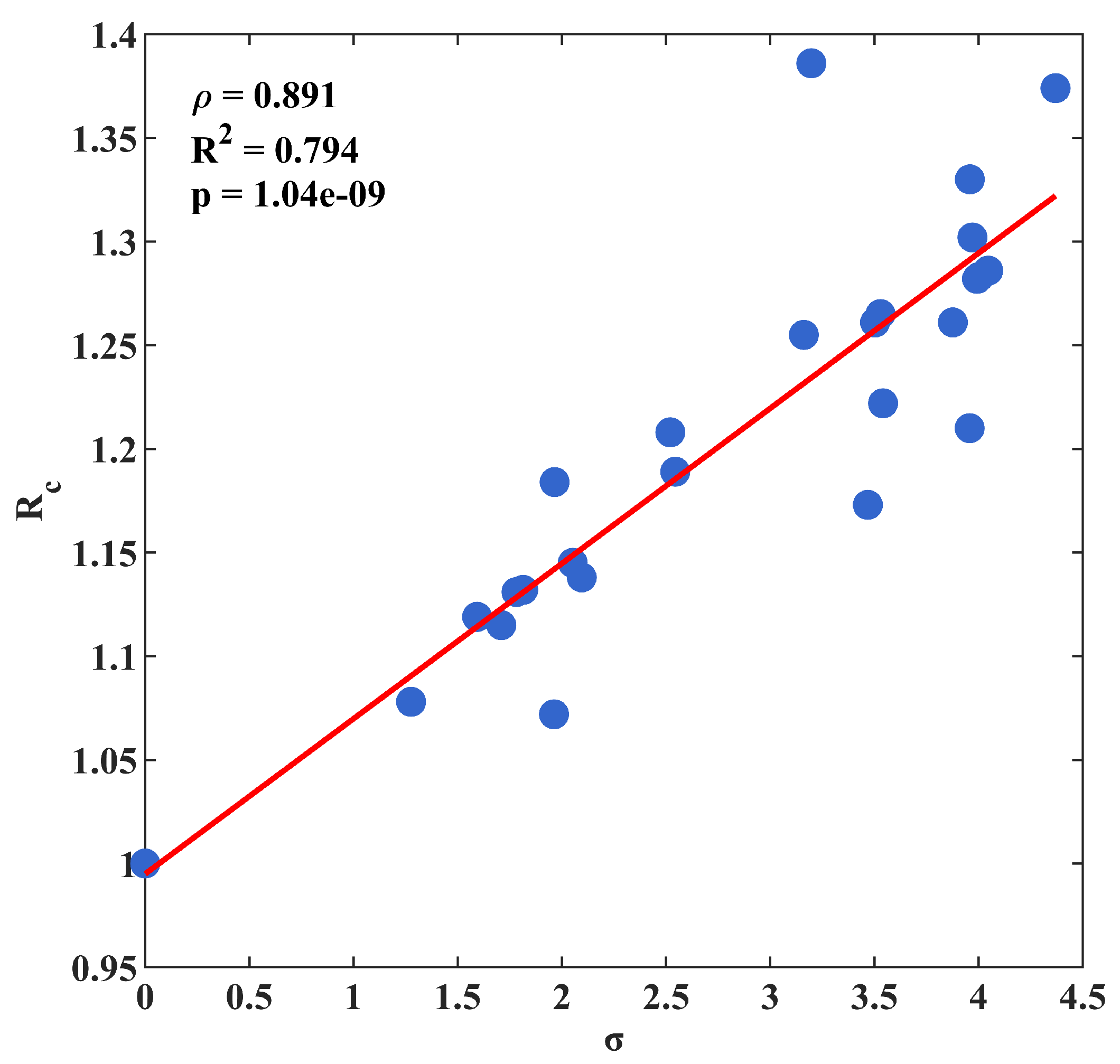
As shown in Figure 10, Spearman correlation analysis revealed a highly significant positive relationship between these two parameters ( r = 0.8911 ,   p < 0.01 ), indicating that R C and σ capture closely related aspects of vertical amplitude in surface microrelief. In contrast, the temporal patterns of fractal dimension D exhibited a different trajectory. On rough panels, D remained relatively stable over time, showing only a slight decrease at 3 to 9 months before recovering to values close to the initial state. On control panels, D increased markedly during the first three months as biofouling developed and then levelled off, converging towards the values observed on rough panels. Thereafter, both panel types clustered around similar values (2.4~2.5) with relatively small dispersion, suggesting convergence once a well-developed fouling canopy had formed (Figure 9c).
Spearman correlation analysis showed that biofouling thickness H was positively correlated with the canopy roughness R C ( r = 0.4233 ,   p < 0.05 ), whereas its correlation with D was not significant ( r = 0.1005 ,   p > 0.05 ). These results indicate that, compared with fractal dimension, canopy roughness is a more effective metric for capturing the influence of surface structure on biofouling development.

4.3. The Flow Characteristics Around the Biofouling Panels

The above analyses demonstrate that engineering rough panels maintain persistently higher canopy roughness and height variability than the control panels, and that these differences are positively associated with biofouling thickness. However, the hydrodynamic mechanisms linking surface morphology to enhanced colonization remain unclear. In particular, it is not known how the observed variations in R C , σ , and D modify the near-bed flow structure, such as the development of upwelling over the panel, the extent of back-eddy recirculation, and the distribution of bed shear stress experienced by settling larvae and growing oysters. In the following section, we relate these flow characteristics to the observed fouling patterns to illustrate the physical mechanisms by which surface morphology promotes or inhibits biofouling on oyster settlement panels.

4.3.1. Relative Flow Velocity Distribution Around Biofouling Panels

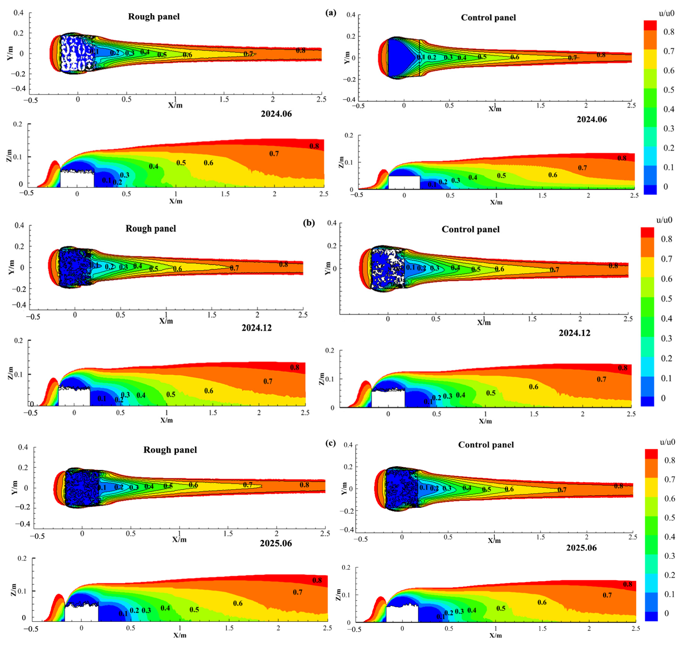
Numerical simulations based on the reconstructed panel geometries reveal that biofouling-induced changes in surface morphology substantially modify the near-bed flow, particularly the strength of upwelling above the panels and the size and intensity of back-eddy recirculation zones. Figure 11 presents the contour plots of the normalized streamwise velocity u / u 0 around rough and control panels at different deployment times. It can be seen that at deployment (June 2024), pronounced differences in the near-bed flow structure were observed between the two panel types. As shown in Figure 11a, in the plan view (XY horizontal plan), above the rough panel, an extensive low-velocity region with u / u 0 0.3 developed immediately downstream of the leading edge, extending both laterally and streamwise. In contrast, the control panel exhibited a much smaller deceleration zone, with higher relative velocities ( u / u 0 0.4 ) dominating most of the wake. The denser packing of low-velocity contours and stronger velocity gradients near the rough panel indicate enhanced flow separation and shear. In the mid-vertical plane (XZ vertical plane), over the rough panel, the low-velocity canopy layer was markedly thicker, with u / u 0 0.3 protruding farther into the water column compared with the control panel. This thicker low-velocity layer and upward bulging of the iso-velocity surfaces point to stronger upwelling and vertical mixing above the rough surface. The control panel, by contrast, was characterized by a thinner, more confined low-velocity layer and a smoother velocity profile. These observations demonstrate that the engineered roughness substantially intensifies near-bed deceleration and vertical exchange at the beginning of deployment, creating a more heterogeneous and turbulent flow environment over the rough panel.
After six months of immersion (Figure 11b), with the development of a fouling canopy on both panel types, the flow fields above the rough and control panels became more similar. In the XY plane, the extent of the u / u 0 = 0.1 ~ 0.3 low-velocity zone immediately downstream of the panel front edge was comparable between treatments. The streaming recovery of the flow towards u / u 0 = 0.7 ~ 0.8 occurred at similar downstream distances. In the XZ plane, both panels were overlain by canopy-scale low-velocity layers of similar thickness. Nevertheless, the rough panel still maintained a slightly thicker low-velocity region and a marginally more pronounced upward deflection of the iso-velocity surfaces, indicating residual enhancement of near-bed mixing relative to the control panel. Thus, biofouling growth progressively masks the initial morphological contrast between the two surfaces, reducing but not eliminating the hydrodynamic differences by month 6.
After 12 months (Figure 11c), when the fouling communities had further developed and formed mature canopies, large-scale flow features over the rough and smooth panels were nearly indistinguishable. The spatial pattern of relative velocity, including the length and lateral extent of the wake, and the position where the streamwise flow recovered to u / u 0 0.8 was almost identical for the two panel types. In the XZ plane, the thickness of the near-bed low velocity layer and the shape of the overlying velocity contours were very similar. Only subtle differences remained: the rough panel retained slightly larger pockets of very low velocity within and immediately behind the canopy, and the near-bed iso-velocity lines showed marginally stronger curvature, implying weakly enhanced micro-scale shear and mixing.

4.3.2. Temporal Evolution of Upwelling and Wake Region Around Biofouling Panels Under Different Deployment Times

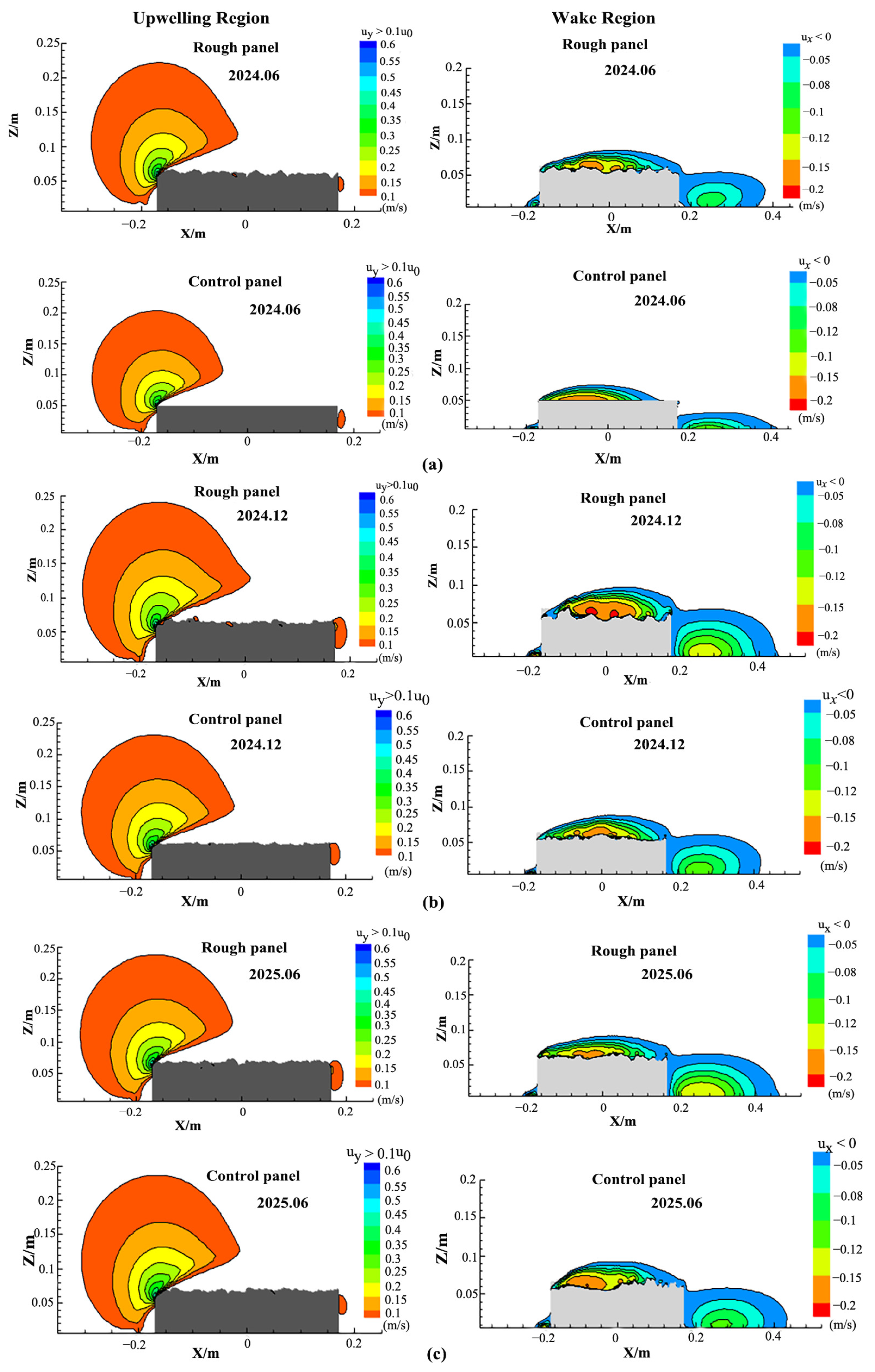
Figure 12 presents the contour plots of vertical velocity and reverse streamwise velocity, together with the integrated upwelling ( u y > 0.1 u 0 ) and wake ( u x < 0 ) volumes, consistently showing that the hydrodynamic contrast between rough and control panels is strongest at deployment and gradually diminishes with time. At an initial deployment, the rough panel generated a much larger and higher upwelling cell above the leading edge than the smooth panel (Figure 12a). This is reflected quantitatively by the upwelling volume, which was about 15~20% higher over the rough panel than over the smooth panel. The normalized upwelling volume ( V u p w e l l i n g / V p a n e l ) was also larger for the rough treatment, indicating that the enhanced upwelling is not solely due to panel size but to the engineered roughness. The reverse flow contours ( u x < 0 ) show an elongated recirculation bubble over the rough panel and a shorter, weaker wake over the control panel. Consistently, both absolute and normalized wake volumes were higher for the rough panels at initial deployment.
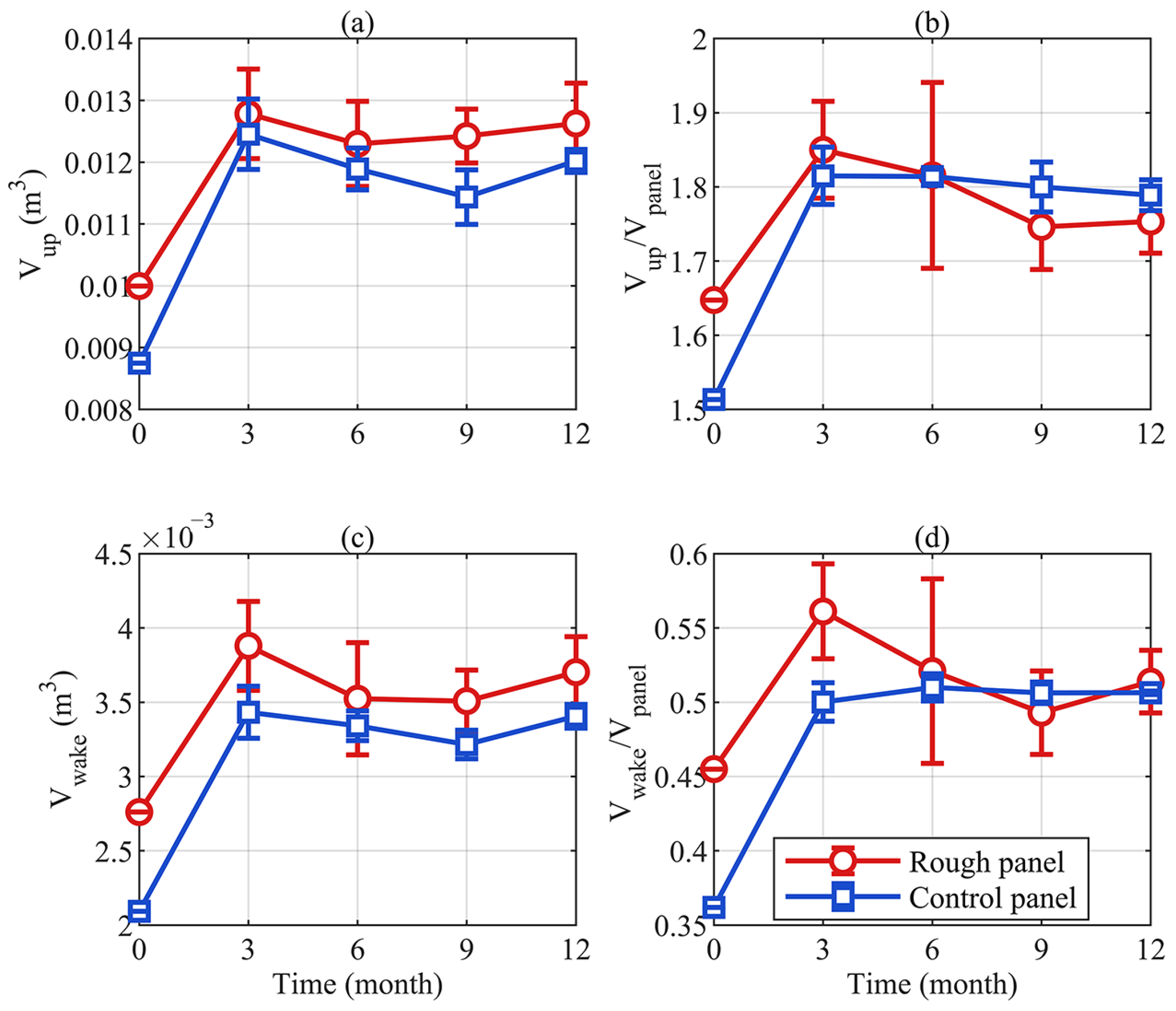
After 3–6 months of deployment, when biofouling canopies had developed on both panel types, the spatial extent of the upwelling region above the rough and control panels became more similar in the section, see Figure 12b. The integrated metrics show that V u p w e l l i n g and V u p w e l l i n g / V p a n e l increased for both treatments from month 0 to 3 and then remained relatively stable, but the difference between rough and smooth panels narrowed markedly (Figure 13a,b). A similar pattern occurred for the wake: wake volume V w a k e over the rough panel peaked at month 3 and then decreased slightly, while the control panel showed a more moderate increase, so that by month 6, the wake volumes and normalized wake volumes V w a k e / V p a n e l of the two treatments almost overlapped (Figure 13c,d). These trends are consistent with the contour plots, which show that the recirculation zones over rough and smooth panels have comparable thickness and downstream extent by month 6.
By 12 months (Figure 12c), with fully developed fouling communities, the upwelling and wake structures over the two panel types were nearly indistinguishable. The vertical sections show similar heights and horizontal extents of the upwelling cells and recirculation zones above rough and control panels. Correspondingly, the time series of integrated volumes indicates that both absolute and normalized upwelling volumes converge to values around V u p w e l l i n g = ( 1.2 1.3 ) × 10 2 m3 and V u p w e l l i n g / V p a n e l 1.75 ~ 1.80 . Wake volumes ( V w a k e ) also converge to ( 3.5 3.8 ) × 10 3 m3 and V w a k e / V p a n e l values of 0.50 for both panel types. As shown in Figure 13a,c, the absolute upwelling and wake volumes above the rough panel are larger than those of the control groups. In contrast, Figure 13b,d present the normalized upwelling volume and wake volume. It can be seen that after 6 months of immersion, the rough panel shows smaller normalized values than the control. This is understandable because the biofouling height ( H ) in Figure 7 on the rough panel is consistently greater than that on the control panel, resulting in a larger overall panel volume for the rough panel.
These results suggest that the engineered micro-roughness of the panels initially enhances vertical mixing and mass transport near the surface by strengthening flow separation and upwelling. This hydrodynamic advantage likely promotes larvae delivery and nutrient supply to the rough panels during the early colonization stage, contributing to their greater biofouling thickness. As biofouling accumulates and the canopies on both panel types converge in height and morphology, the simulated upwelling characteristics also converge, implying that the hydrodynamic contrast between rough and smooth treatments becomes progressively weaker at later stages of community development.

4.3.3. Wall Shear Stress Distribution on the Biofouled Panel Surfaces

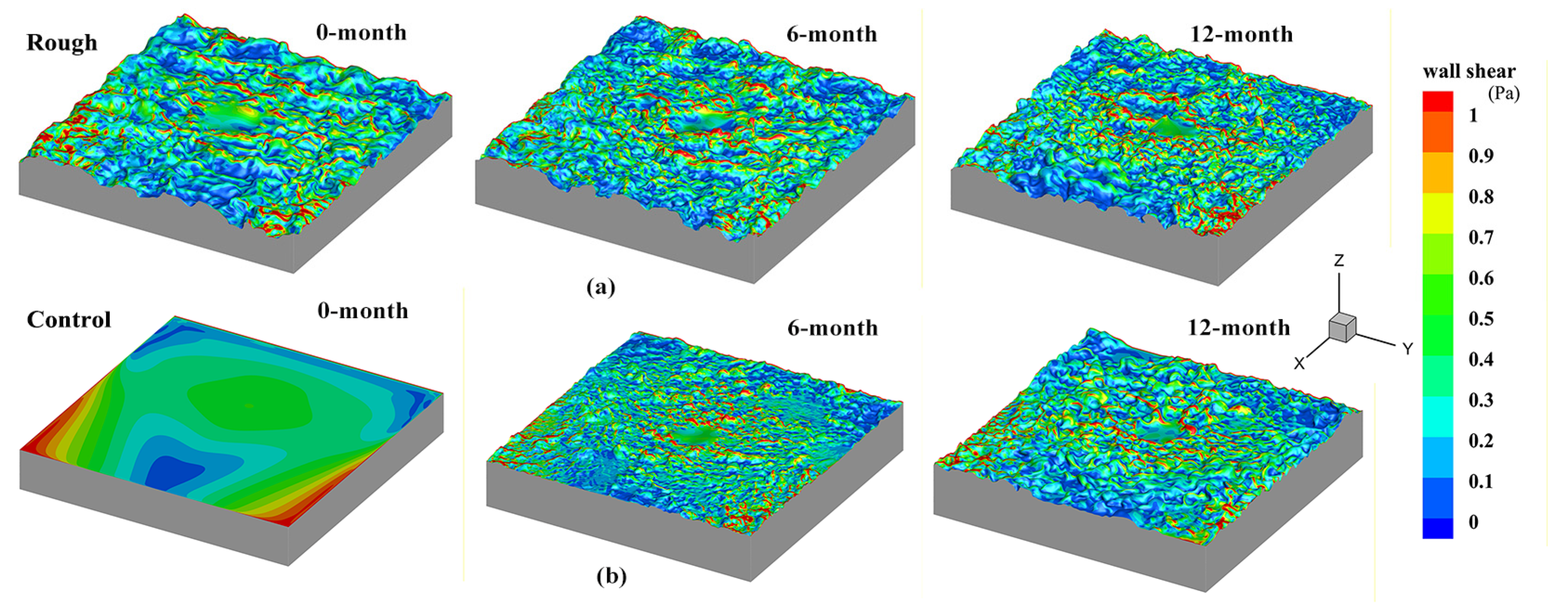
Figure 14a,b further compares the evolution of wall shear stress on the initially rough panels and on the smooth concrete control panels. The top row shows the rough panels at 0, 6, and 12 months, while the bottom row shows the corresponding cases for the control panels. All subplots use the same color scale for wall shear stress τ p (0–1.0 P a ). For the initial rough panel, the 0-month surface already exhibits pronounced small-scale variability in τ p , with alternating high- and low-shear streaks associated with the underlying manufactured roughness. As biofilm accumulates and the roughness elements grow, biofilm growth partly fills the smaller depressions and modifies the crests, leading to a redistribution rather than a simple increase in shear: some former high-shear spots are attenuated, whereas new high-shear patches appear around the tops and upstream faces of the developing biofilm structures. By 12 months, the rough panels display a very intermittent pattern, with elongated high-shear ridges embedded in a background of moderated shear, reflecting the complex multi-scale morphology of the mature fouling layer. Overall, the rough panels show both an increase in the area-averaged shear stress and a pronounced enhancement of spatial variability. For the smooth control panels, the 0-month surface is nearly hydrodynamically smooth: the shear-stress distribution is dominated by a broad, large-scale gradient and lacks localized high-shear stress. After 6 months of immersion, a thin and spatially patchy biofilm layer develops, and small-scale variations start to emerge, especially near the edges and isolated protrusions. By 12 months, the control panels are also covered by an irregular fouling layer, and their shear-stress field becomes much more structured, with discrete high-shear patches similar in magnitude to those on the rough panels. Nevertheless, the control panels retain larger contiguous areas of low shear and a narrow overall range of τ p , indicating that biofilm growing on an originally smooth substrate generates weaker and less intermittent shear than on the pre-roughened panels.
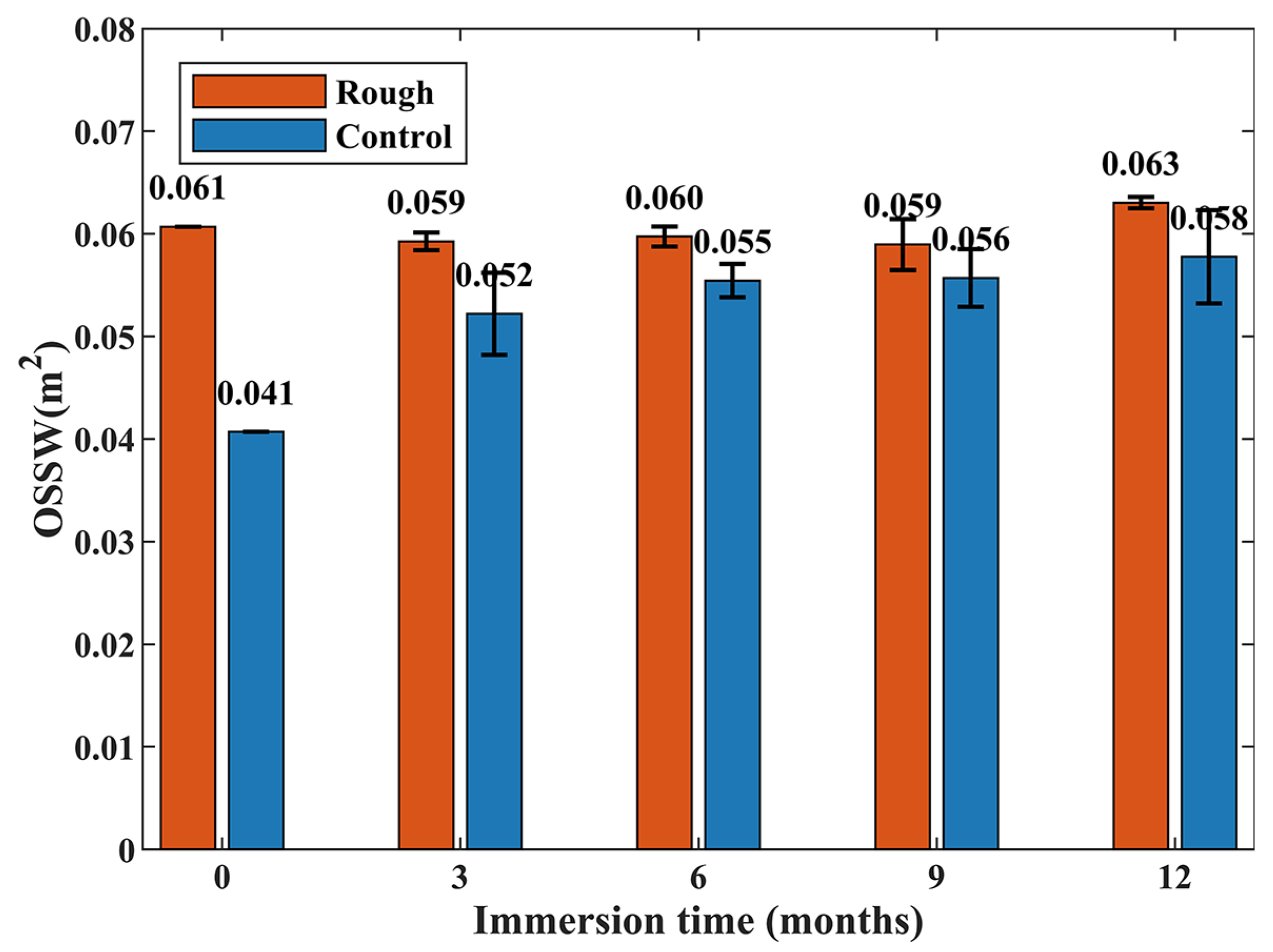
Following previous studies on hydrodynamic controls on oyster larval settlement [46,47], we operationally defined an “Oyster Settlement Shear-Stress Window” (OSSW) as the range of 0.05–0.30 Pa. This range is used here as a literature-informed proxy for hydraulically favorable settlement conditions, rather than as a site-specific threshold calibrated directly with settlement measurements on the present panels. Shear stresses above approximately τ p 0.4 0.5   P a have been reported to enhance resuspension and reduce post-settlement survival, whereas very low shear may limit mass transfer of oxygen and food. For each panel and sampling time, we extracted the portion of the panel surface whose shear stress falls within 0.05–0.30 Pa and calculated the corresponding OSSW area. Accordingly, the OSSW should be interpreted as a comparative indicator of potential settlement suitability under different surface morphologies, rather than a direct measurement of realized larval settlement. Figure 15 provides the temporal evolution of the OSSW area for the rough and control panels. At all immersion times, the rough panels provide more surface area within the optional window than the control panels. At 0 months, the OSSW area on the rough panels is already about 0.0607 m2, compared with only 0.0407 m2 on the control smooth panel. This is consistent with the initial shear-stress contours, where the manufactured roughness produces a broad band of moderate shear, interspersed with only limited localized high-shear stress regions. As biofilm develops on the control panels (3–12 months), the OSSW area increases from 0.0407 m2 to 0.0578 m2. The biofouling growth increases the OSSW area on control panels. For the rough panels, the OSSW area remains high (0.059~0.063 m2) throughout the immersion period, with only minor fluctuations. Although biofilm growth enhances local shear heterogeneity and produces strong high-shear ridges, it simultaneously creates sheltered low-shear pockets. The net effect is that a substantial fraction of the surface persistently falls within the 0.05–0.30 Pa window.
Combining the shear stress distribution contours (Figure 14) and the OSSW statistics indicates that initially rough panels not only generate a stronger shear stress region, but also offer a larger and more persistent area of hydraulically optimal conditions for oyster larval attachment than smooth panels. Smooth panels become more favorable only after sufficient biofilm has accumulated to roughen the surface and redistribute the local shear. Thus, the OSSW analysis bridges the purely hydrodynamic description of shear-stress distributions with their ecological relevance, providing a quantitative measure of how panel type and biofouling development jointly control the availability of suitable settlement area for oyster larvae.

4.3.4. Vortex Distribution Characteristics

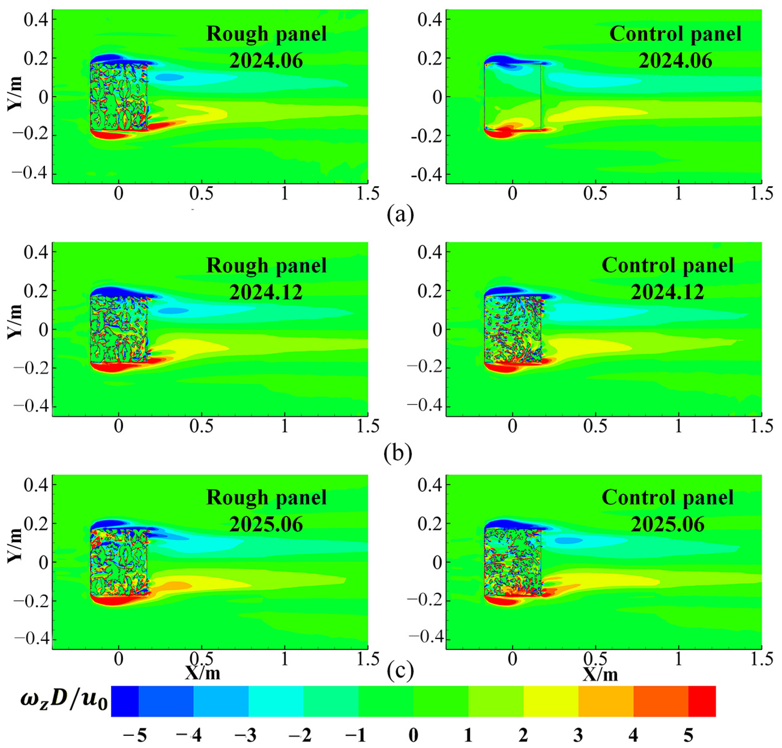
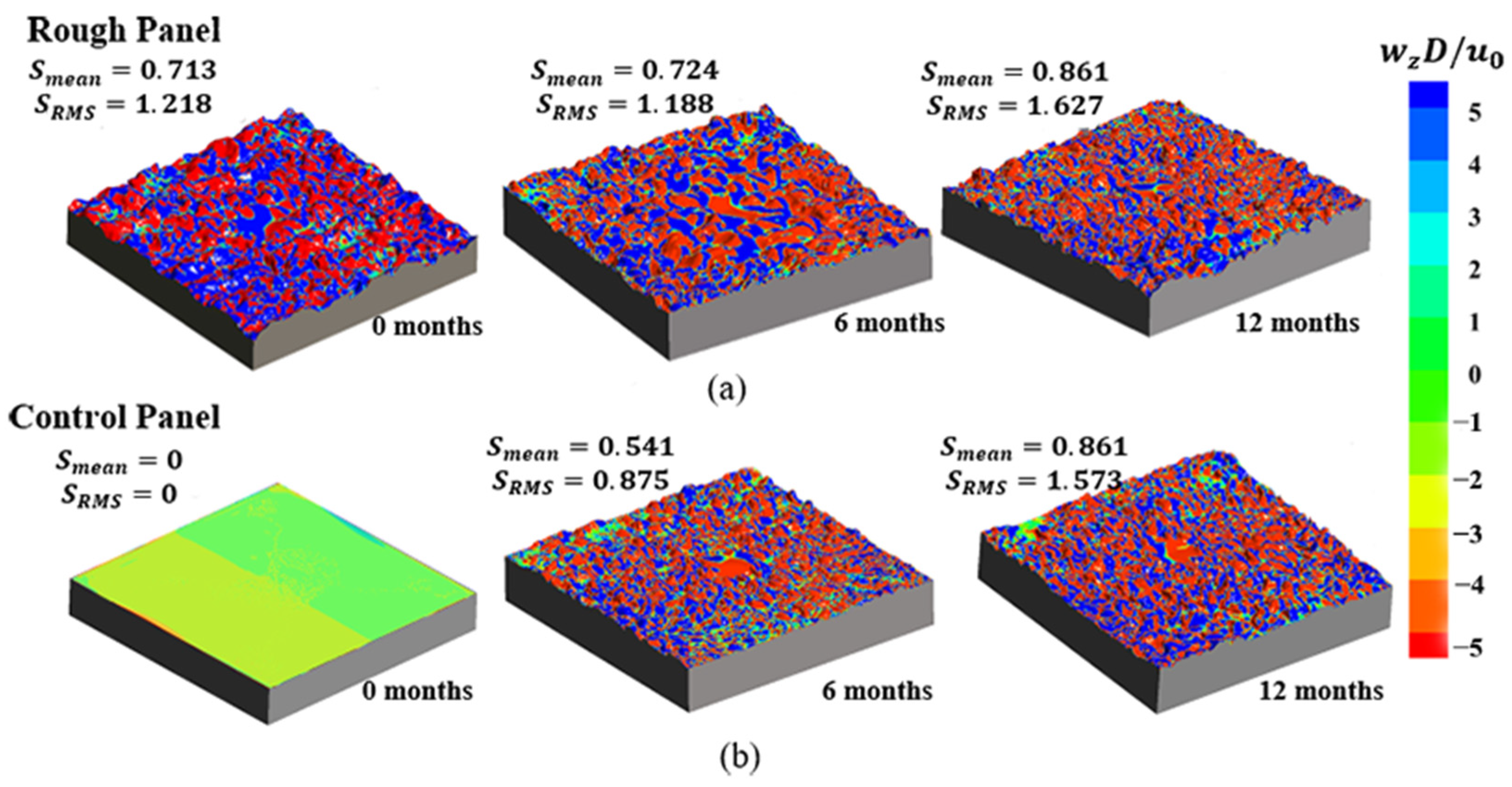
Figure 16 compares the distribution of the normalized spanwise vorticity ( ω z D / u 0 ) in a horizontal section (the XY plane) for the rough and control panels at the three immersion stages. All plots use the same color scale [−5, 5] to allow a direct quantitative comparison between cases. As shown in Figure 16a, the patchy high-magnitude vorticity regions are spatially correlated with the roughness elements resolved in the surface topography. In contrast, the smooth control panel shows a much more uniform, nearly low vorticity field with only a weak, narrow shear layer developing along the obstacle edges. This confirms that the higher roughness amplitude and slope of the rough panel do not merely perturb the mean flow but generate a dense population of small-scale vortices in the near-wall region. These vortical structures provide an efficient mechanism for momentum exchange between the near-wall low-momentum fluid and the outer flow.
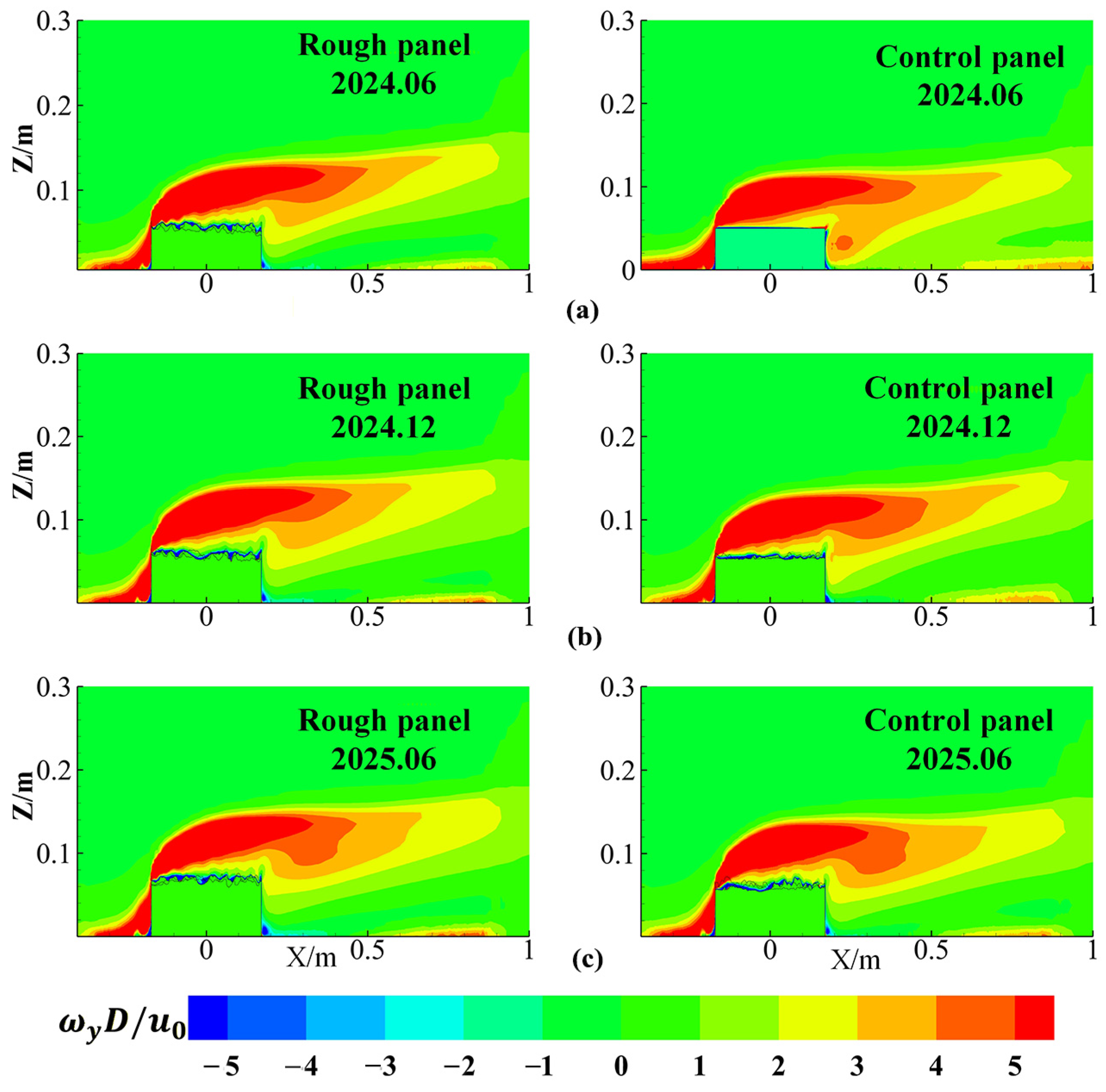
Figure 17 further illustrates how the roughness-induced vortices modify the separated shear layer downstream of the panel. For the rough panel, a strong negative ω y D / u 0 layer forms at the edge and expands more rapidly in the wall-normal direction compared with the control case. The high-magnitude vorticity core is thicker, and its peak value is slightly larger, consistent with the enhanced shear and mixing inferred from the higher roughness indices. The region of intense also decays somewhat earlier in the streamwise direction, indicating a shorter separation bubble and an upstream shift in the reattachment point.

5. Discussion

This study focuses on establishing a quantitative link between the dynamic development of biofouling roughness and the hydrodynamic conditions that control early oyster settlement. Specifically, we used offshore hanging-panel experiments and 3D scanning to characterize how the temporal changes in biofouling thickness ( H ), canopy roughness ( R C ), surface heterogeneity ( σ ), and fractal dimension ( D ) modify panel-scale roughness. Second, we employed CFD simulations to resolve how these micro-structural metrics regulate the surrounding flow field, including relative flow velocity, upwelling and wake regions, wall shear stress, and vorticity around and on the panels. Third, we derive a shear-stress-based habitat metric (the area of panel surface within an oyster-relevant optimal shear-stress window) and demonstrate its systematic relationship with canopy roughness. The key contribution of this work is to move from qualitative notions of “complex structure promotes settlement” [48] to a mechanistic, quantifiable relationship between canopy roughness, wall shear-stress distribution, and the potential habitat area for oyster larval settlement.

5.1. Overall Hydrodynamic Effects of Biofouling Roughness

The progressive development of biofilm and canopy-forming fouling organisms exerts a first-order control on the near-field hydrodynamics around the panels. With increasing deployment time, the panels evolve from relatively smooth surfaces to highly irregular roughness canopies, accompanied by systematic changes in velocity, wake, and shear-stress patterns (Section 4.1, Section 4.2 and Section 4.3). These patterns are consistent with the general behavior of turbulent flows over rough walls, where increased roughness height and density amplify form drag, alter the structure of near-wall turbulence, and intensify momentum exchange [41]. Turbulence over rough reef substrates can trigger active downward propulsion of oyster larvae, increasing larval-substrate contact probability [46], which provides a plausible mechanistic basis for the higher biomass observed on roughened panels in our field experiment.
To link the simulated hydrodynamics with habitat suitability, we defined an optimal wall-shear-stress window for oyster settlement (OSSW) of 0.05–0.30 P a , based on previous work indicating that stresses above 0.40–0.5 P a promote dislodgement, whereas some level of flow is required for oxygen and food delivery [32,47]. For each experimental and control panel, we calculated the surface area with local shear stress within this range. At all deployments, rough panels consistently exhibit larger OSSW than control panels, despite also generating stronger shear hotspots. As biofilm growth roughens initially smooth panels, their OSSW increases, indicating that biological colonization progressively converts hydraulically unfavorable smooth substrates into more settlement-friendly roughness canopies.
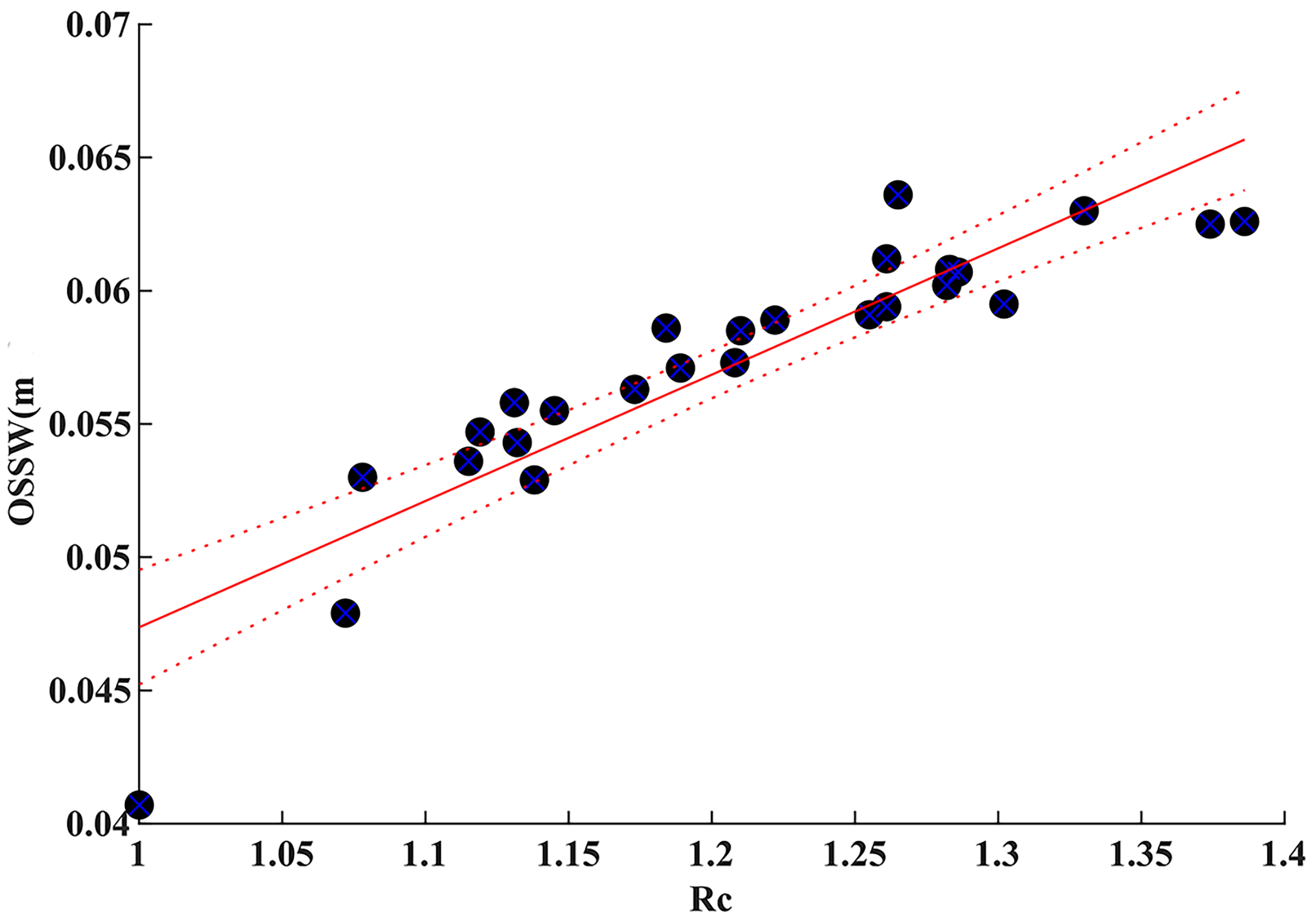
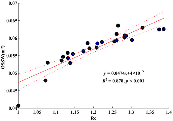
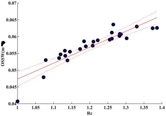
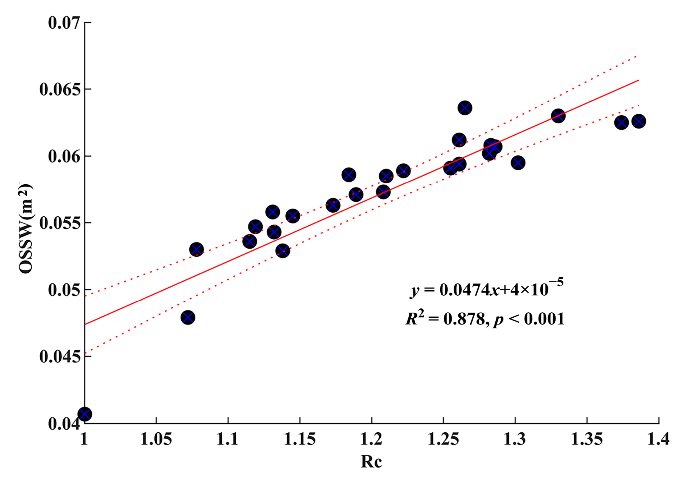
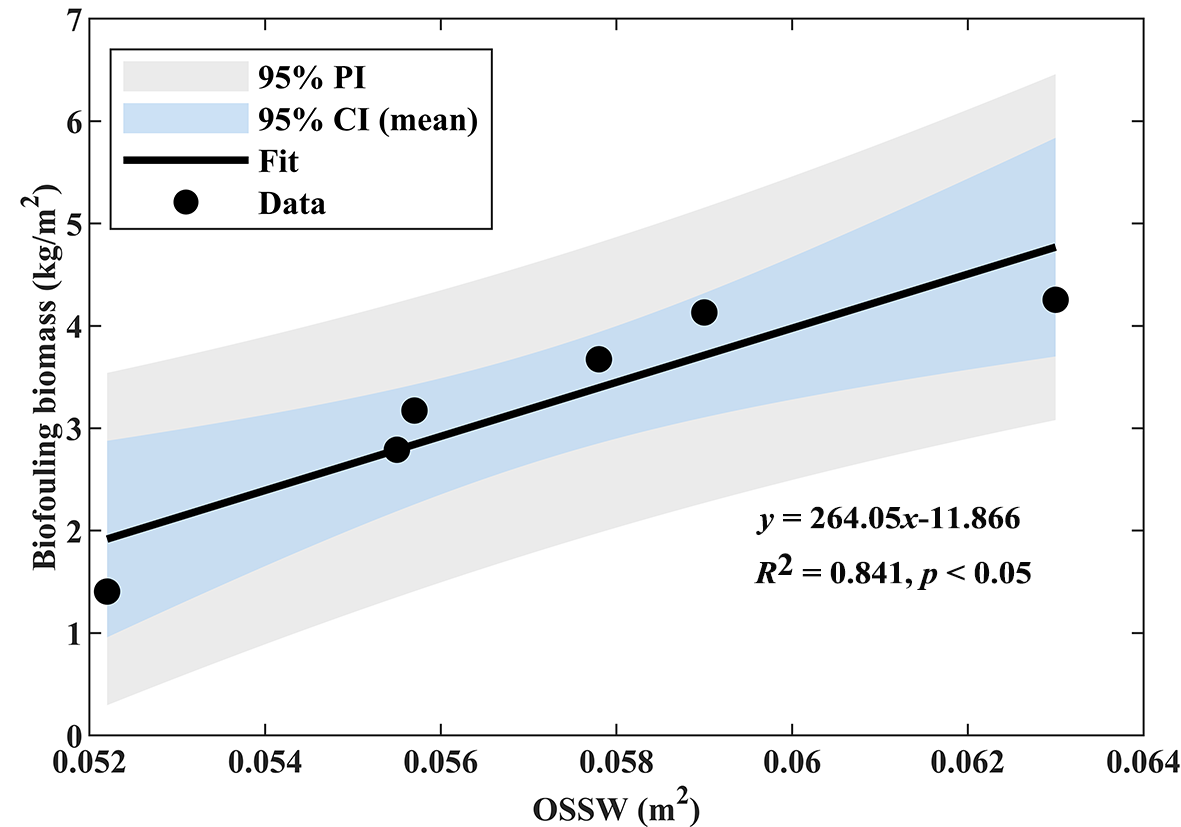
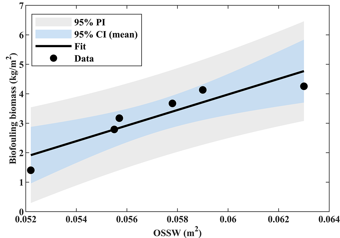
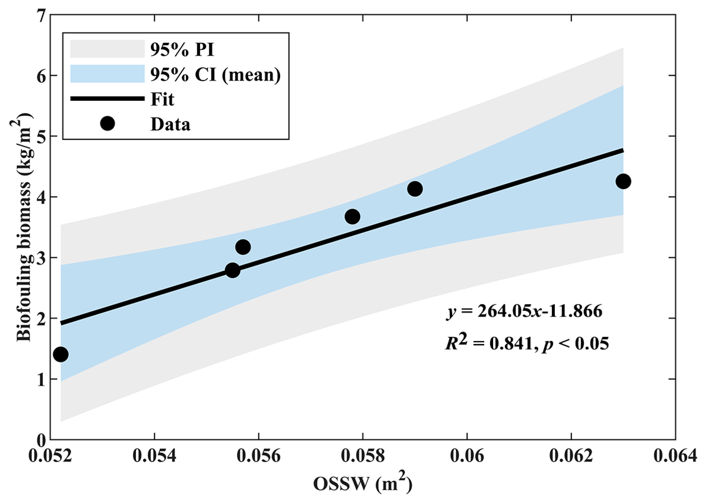
The significant positive linear relationship between R C and OSSW (Figure 18, R 2 = 0.878 ,   p < 0.001 ) indicates that increasing canopy roughness enhances the formation of hydraulically heterogeneous microhabitats. In other words, rougher canopies are more effective at transforming the incoming flow into a more spatially variable wake structure. The red dashed line represents the linear regression fit between R C and OSSW. This result is consistent with the recent work by Cannon et al. [34], who showed that the rugosity index R C and structural complexity of natural and restored oyster canopies, is closely linked to their hydrodynamic influence, including enhanced drag and flow attenuation within the reef [49,50]. Our CFD simulation results extend these field-scale observations to the panel scale and explicitly connect a similar roughness metric to the creation of settlement-relevant shear environments. In Section 4.1, we obtained the linear relationship between R C and biofouling biomass, while Figure 19 shows a positive relationship between the OSSW area and biomass. A significant positive linear relationship was observed between OSSW and biofouling biomass (Figure 19, R 2 = 0.841, p   < 0.05 ). Similar to the findings of Lanham et al., these results suggest that deliberately engineering surface roughness on artificial reefs can increase biofouling biomass and thereby create more favorable microhabitats for oyster settlement and subsequent development [36].
Note that R C has a theoretical minimum value of 1, representing a smooth surface. For OSSW, although its value is always greater than zero in this study because it is calculated from the cumulative distribution of wall shear stress over the panel surface, the x-axis in Figure 19 does not represent a theoretical lower bound. Instead, it was set according to the observed data range (approximately 0.052–0.063 m2) to better visualize the linear relationship between OSSW and biofouling biomass. This choice of axis range is for graphical clarity only and does not affect the regression analysis or statistical significance.

5.2. Local Slope, Micro-Topography, and Shear-Stress Heterogeneity

Existing studies indicate that oyster larvae settlement is not a random process, but is strongly biased toward micro-habitats where near-bed velocity and turbulence are substantially attenuated, particularly within crevices or highly complex roughness elements on natural and artificial reefs [29,47]. Intense turbulent shear markedly reduces larval residence time in the vicinity of the bed and therefore suppresses successful colonization [32]. In contrast, intermediate substrate roughness introduces micro-topographic sheltering that reduces near-bed shear stress and turbulent stress events locally, increasing larval retention and the probability of attachment [31,33].
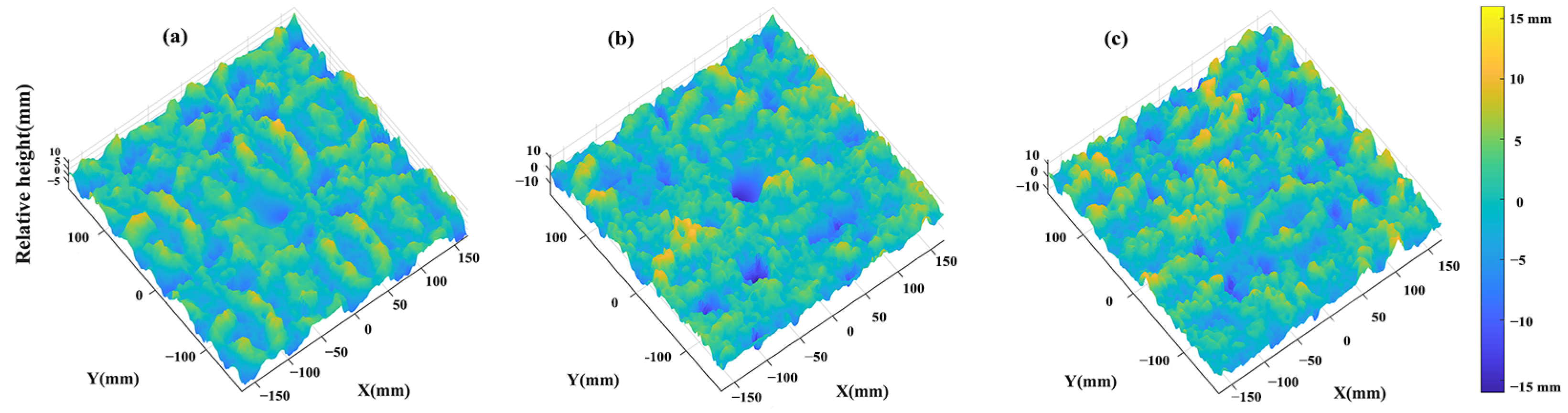
Figure 20 presents the relative biofouling height contours of the rough panels at 0, 6, and 12 months. The temporal evolution of the rough panels is clearly visible in the 3D height maps. After removal of the best-fit plane, the initial panel exhibits only low-amplitude, relatively uniformly distributed height variations, whereas with increasing deployment time, the surface develops pronounced peaks and depressions and a patchier height distribution. This progressive increase in relief and micro-topographic contrast translates into steeper local slopes on exposed elements and deeper, more frequent concavities between them.
Figure 21 provides the local slopes S m e a n and S R M S of these biofouled panels at different immersion stages. The surface-slope statistics further confirm the temporal evolution of the roughness geometry. For the rough panel at the initial deployment, the mean slope and RMS slope are S m e a n = 0.713 ,   S R M S = 1.218 , respectively. After 12 months of immersion, both metrics increase to S m e a n = 0.861 ,   S R M S = 1.627 . This systematic increase indicates that the roughness elements become not only higher but also noticeably steeper and more irregular with time. In particular, the growth in S R M S reflects a broader distribution of local inclinations and sharper surface features, which is consistent with the stronger wall-shear stress concentrations and the more intense near-wall vorticity observed in the velocity and vorticity fields for the one-year immersion.
As shown in Figure 16 and Figure 17, our simulation results clarify how specific aspects of micro-topography, especially local slope, contribute to this hydrodynamic heterogeneity. Steep, upstream-facing elements experience elevated near-wall velocity and high wall shear stress, forming a localized high shear-stress region that is prone to scour and larvae removal. In contrast, leeward faces, depressions, and inter-canopy gaps promote local flow separation and recirculation, yielding pockets of reduced velocity, weakened turbulence, and lower shear stress. The vortex distribution further shows that coherent vortices are preferentially shed from steep roughness elements, while concave or gently sloping features mainly host small-scale eddies with limited erosive capacity (see Figure 21a,b).
These mechanisms are consistent with experimental work on settlement substrates. Marine et al. found that Ostrea edulis recruitment on concrete panels was strongly controlled by surface texture and micro-topography: rough, irregular, and slightly concave surfaces supported substantially higher settlement than smooth profiles, which the authors attributed to enhanced local retention and reduced shear [19]. As shown in Figure 11, Figure 16 and Figure 17, our simulations provide a hydrodynamic explanation for these observations by showing that similar micro-topographic features on biofouled panels act as low-shear refugia, while the surrounding flow remains relatively fast and turbulent.

5.3. Comparison with Reef-Scale Studies and Implications for Eco-Engineering

Field studies on artificial and natural oyster reefs have highlighted the broader geomorphic and ecological consequences of adding three-dimensional roughness to coastal environments. In the Bohai Sea, artificial oyster reefs increased structural complexity, improved trophic structure, and enhanced coastal ecosystem functions compared with adjacent soft-bottom habitats [18]. Walles et al. (2016) showed that artificial reefs of Crassostrea gigas developed into self-sustaining structures that trap sediment, alter local hydrodynamics, and provide habitat for diverse benthic communities [51]. Scyphers et al. (2011) demonstrated that oyster-shell breakwaters can attenuate wave energy, reduce shoreline erosion, and substantially increase fish and crab abundances [9].
These studies mainly focus on reef-scale responses, whereas our work operates at the panel scale and resolves centimetre-scale shear and vortex patterns. Nevertheless, the underlying mechanisms are consistent: adding rough, canopy-forming structures reorganises the flow into sheltered and exposed zones, thereby enhancing both habitat availability and coastal-protection functions. After one year of immersion, the fouled rough panels ( R c = 1.374 ,   σ = 4.369 ,   s = 1.627 ) generated an upwelling volume 1.45 times that of the initially smooth control panels ( R c = 1 ,   σ = 0 ,   s = 0 ), while the wake volume was increased by a factor of 1.81. By explicitly linking a measurable roughness index R C to the production of moderate-shear micro-habitats, our results offer a hydrodynamic criterion that complements structural metrics such as rugosity or fractal dimension commonly used in reef assessments [34].
From an engineering perspective, these findings support design approaches that prioritise surface complexity and suitable flow environments rather than material choice alone. Substrates that combine moderate relief, irregular micro-topography, and frequent crevices—whether formed by biofouling or engineered directly into artificial units—are likely to maximize the area of hydraulically favorable habitat while avoiding excessively steep elements that generate large shear hotspots. Such configurations may provide an optimal trade-off between promoting larvae settlement and limiting post-settlement erosion, and are therefore highly relevant for the design of eco-engineered panels, artificial reefs, and hybrid grey–green coastal structures [19,51].

5.4. Limitations and Future Work

In our present study, several limitations should be acknowledged. Although this study revealed clear relationships among canopy roughness, OSSW, and biofouling biomass at the Xiangyun Bay site, the extrapolation of these results to other locations should be made cautiously. Site-specific differences in hydrodynamics, water quality, and ecological conditions may influence the strength and form of these relationships. The numerical simulations are based on steady inflow and a specific turbulence closure, and do not resolve the full spectrum of unsteady events, wave–current interactions, or extreme flows that can contribute to episodic scour. Biofouling was represented as a rigid canopy, whereas real fouling organisms can deform or reconfigure under flow, potentially altering both drag and near-bed shear [52].
Future work should therefore couple high-resolution hydrodynamic modelling with laboratory or field experiments that quantify actual settlement and post-settlement survival on substrates with systematically varied roughness characteristics. Incorporating flexible or poroelastic representations of fouling canopies would improve understanding of flow–structure interactions, while extending the analysis across different flow regimes and species would help test the generality of the roughness–shear–settlement relationships identified here and refine design guidelines for eco-engineered coastal infrastructure.

6. Conclusions

In this study, we combined field panel experiments, 3D surface characterization, and CFD modelling to investigate how biofouling-induced roughness regulates the near-wall flow environment over artificial oyster reef substrates. The main conclusions are as follows:
(1)
Temporal evolution of biofouling thickness
Throughout the 12-month immersion, panels with initial rough textures consistently exhibited a higher biofouling thickness ( H ) and biomass than the smooth control panels. Both rough and control panels developed substantial biofouling layers, with H of 6.39 mm and 5.91 mm, respectively. The biomass showed a significant linear relationship with H , indicating that thickness can be used as a reliable proxy for the accumulation of attached biomass on the panels.
(2)
Changes in surface-morphology indices
The canopy roughness R C , surface heterogeneity σ generally increased with immersion time, reflecting the progressive roughening of panel surfaces by biological growth. Rough panel consistently exhibited higher R C and σ than control panels, and these two indices showed a strong linear correlation ( R 2 = 0.891 ). By contrast, the temporal patterns of fractal dimension D differed between panel types. D of the rough panels showed a slight decrease during the early immersion period and then stabilized, whereas the smooth panels experienced a marked increase in D as biofouling developed. This divergence indicates that while biofouling accumulation enhances small-scale complexity on initially smooth surfaces, it can partially fill pre-existing cavities and asperities on rough panels, thereby smoothing their finest features.
(3)
Hydrodynamic response to roughness and biofouling
CFD simulation results demonstrate that increased canopy roughness enhances upwelling and wake development around the fouled panels and modifies the distribution of surface shear-stress of the fouled panels. The area of the oyster settlement shear-stress window (OSSW) expands with increasing R C , indicating that rougher, biofouled surfaces generate more suitable hydrodynamic conditions for oyster settlement and growth.
(4)
Co-evolution of roughness and flow habitat
With continued immersion, the hydrodynamic differences between initially rough and smooth panels gradually diminish, as biofouling accumulation increases the effective roughness of smooth panels. This finding suggests that biological growth can progressively “naturalize” engineered substrates, reducing the contrast between artificial and reef-like surfaces in terms of their hydrodynamic habitat quality.
Overall, the integrated morphological and numerical analyses provide a quantitative basis for incorporating reef-like surface roughness into the design and optimization of artificial oyster reefs and other habitat-enhancing coastal structures. Appropriate control of initial surface roughness, in combination with expected biofouling development, can be used to tailor local flow conditions to the requirements of target species.

Author Contributions

Conceptualization, X.W. and Y.M.; methodology, Y.M. and S.S.; software, Y.M. and X.W.; validation, Y.M., S.S. and X.W.; formal analysis, Y.M., S.S. and H.L.; investigation, Y.M., S.S., H.L. and M.L.; resources, X.W. and Y.T.; data curation, Y.M. and S.S.; writing—original draft preparation, Y.M.; writing—review and editing, X.W. and S.S.; visualization, Y.M.; supervision, X.W.; project administration, X.W.; funding acquisition, Y.T. and X.W. All authors have read and agreed to the published version of the manuscript.

Funding

This research was mainly funded by the National Key Research and Development Program of China (2023YFD2401102), and partially supported by China Three Gorges Renewable (Group) Co., Ltd., No. 37022078 (The funder was not involved in the study design, collection, analysis, interpretation of data, the writing of this article, or the decision to submit it for publication).

Data Availability Statement

The code for the data analysis is available upon request from the authors.

Conflicts of Interest

The authors declare no conflicts of interest.

Appendix A. Grid Independence and Turbulence Model Validation
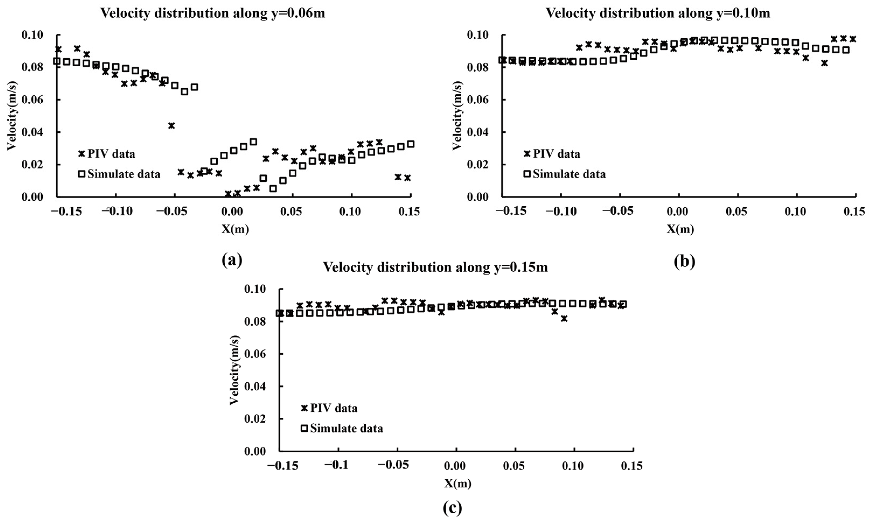
In this study, the turbulence model was validated by comparing the simulation results of the open-cube reef model with Particle Image Velocimetry (PIV) experimental data [44]. Panels a–c of Figure A1 show the velocity distributions along y = 0.06, 0.10, and 0.15 m, respectively. As shown in Figure A1, at all three characteristic sections, the numerical simulation results generally reproduced the experimentally measured velocity trends well. Near the opening region of the reef model, the velocity profiles exhibited more pronounced fluctuations, indicating that the local flow was strongly disturbed by the reef structure. As the measurement sections moved farther away from the reef, the velocity distributions gradually became smoother, and the agreement between the simulated and experimental results further improved. Overall, the simulated results were in good agreement with the PIV data in terms of both the velocity magnitude in the main flow region and the local fluctuation characteristics, indicating that the established numerical model can accurately capture the flow characteristics around the open-cube reef. Therefore, the numerical approach adopted in this study, including the k–ω SST turbulence model, the Fluent meshing strategy using Mosaic poly-Hexcore grids, and similar boundary conditions, can be used to simulate the flow around artificial oyster reef models.
Figure A1. Comparison of the flow and velocity distribution line between the PIV model and numerical model: (a) is the velocity curve along y = 0.06 m; (b) is the velocity curve along y = 0.1 m; (c) is the velocity curve along y = 0.15 m.
Jmse 14 00703 g0a1
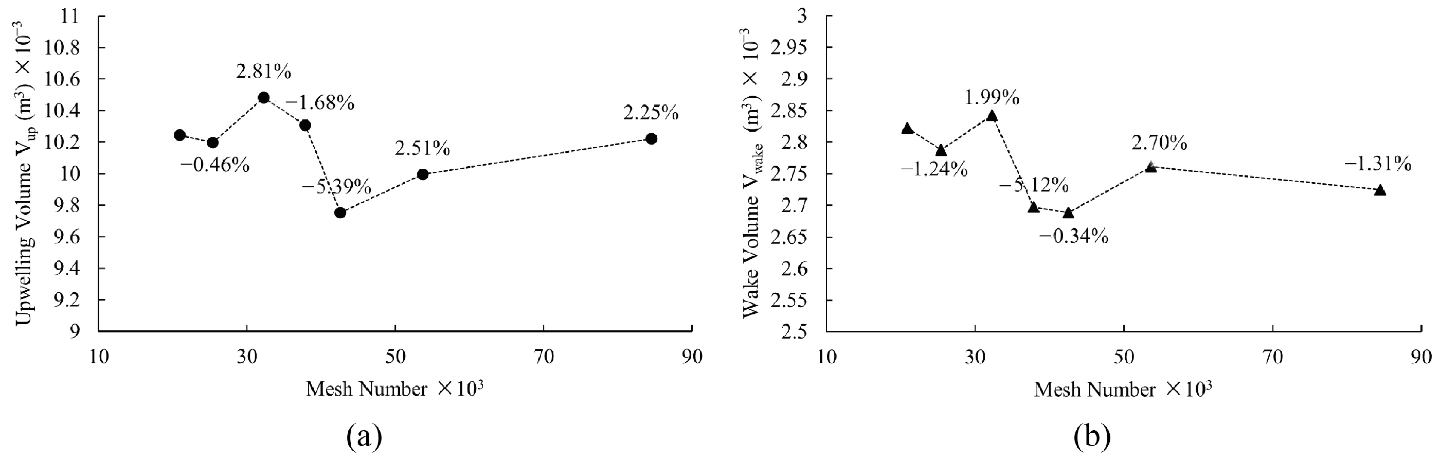
To verify grid independence, a mesh sensitivity analysis was conducted in this study. Figure A2 presents the simulated flow field results for the substrate without biofouling in the experimental group. The horizontal axis represents the total number of mesh elements, while the vertical axis indicates the upwelling volume and wake volume. As shown in Figure A2 and Table A1, when the total number of mesh elements reaches approximately 5.4 million, and the minimum mesh size in the refined region is 0.85 mm, the key flow field parameters tend to stabilize, indicating that the grid independence requirement has been satisfied. This mesh configuration ensures simulation accuracy while maintaining computational efficiency and is therefore suitable for subsequent hydrodynamic analyses.
Figure A2. Mesh sensitivity analysis test: (a) Changes in upwelling volume and (b) wake volume with the number of grid computational cells.
Jmse 14 00703 g0a2
Table A1. The grid parameters used for the sensitivity analysis.
Minimum Mesh Size (mm)Mesh NumberUpwelling Volume (m3)ResidualWake Volume (m3)Residual
1.72,091,3050.01024-0.00282-
1.532,541,8800.01020−0.46%0.00279−1.24%
1.363,226,7530.010482.81%0.002841.99%
1.194,256,1550.01031−1.68%0.00270−5.12%
1.023,786,0510.00975−5.39%0.00269−0.34%
0.855,368,8030.010002.51%0.002762.70%
0.688,448,2450.010222.25%0.00272−1.31%

References

  1. Komyakova, V.; Chamberlain, D.; Jones, G.P.; Swearer, S.E. Assessing the performance of artificial reefs as substitute habitat for temperate reef fishes: Implications for reef design and placement. Sci. Total Environ. 2019, 668, 139–152. [Google Scholar] [CrossRef] [PubMed]
  2. Lima, J.S.; Zalmon, I.R.; Love, M. Overview and trends of ecological and socioeconomic research on artificial reefs. Mar. Environ. Res. 2019, 145, 81–96. [Google Scholar] [CrossRef]
  3. Becker, A.; Taylor, M.D.; Folpp, H.; Lowry, M.B. Managing the development of artificial reef systems: The need for quantitative goals. Fish Fish. 2018, 19, 740–752. [Google Scholar] [CrossRef]
  4. Grabowski, J.H.; Brumbaugh, R.D.; Conrad, R.F.; Keeler, A.G.; Opaluch, J.J.; Peterson, C.H.; Piehler, M.F.; Powers, S.P.; Smyth, A.R. Economic valuation of ecosystem services provided by oyster reefs. BioScience 2012, 62, 900–909. [Google Scholar] [CrossRef]
  5. Filippini, G.; Dafforn, K.A.; Bugnot, A.B. Shellfish as a bioremediation tool: A review and meta-analysis. Environ. Pollut. 2023, 318, 120614. [Google Scholar] [CrossRef]
  6. Hoellein, T.J.; Zarnoch, C.B.; Grizzle, R.E. Eastern oyster (Crassostrea virginica) filtration, biodeposition, and sediment nitrogen cycling at two oyster reefs with contrasting water quality in Great Bay Estuary (New Hampshire, USA). Biogeochemistry 2015, 122, 113–129. [Google Scholar] [CrossRef]
  7. McClenachan, G.M.; Donnelly, M.J.; Shaffer, M.N.; Sacks, P.E.; Walters, L.J. Does size matter? Quantifying the cumulative impact of small-scale living shoreline and oyster reef restoration projects on shoreline erosion. Restor. Ecol. 2020, 28, 1365–1371. [Google Scholar] [CrossRef]
  8. Morris, R.L.; Bilkovic, D.M.; Boswell, M.K.; Bushek, D.; Cebrian, J.; Goff, J.; Kibler, K.M.; La Peyre, M.K.; McClenachan, G.; Moody, J. The application of oyster reefs in shoreline protection: Are we over-engineering for an ecosystem engineer? J. Appl. Ecol. 2019, 56, 1703–1711. [Google Scholar] [CrossRef]
  9. Scyphers, S.B.; Powers, S.P.; Heck, K.L.; Byron, D. Oyster reefs as natural breakwaters mitigate shoreline loss and facilitate fisheries. PLoS ONE 2011, 6, e22396. [Google Scholar] [CrossRef]
  10. Gain, I.E.; Brewton, R.A.; Reese Robillard, M.M.; Johnson, K.D.; Smee, D.L.; Stunz, G.W. Macrofauna using intertidal oyster reef varies in relation to position within the estuarine habitat mosaic. Mar. Biol. 2017, 164, 8. [Google Scholar] [CrossRef]
  11. zu Ermgassen, P.S.E.; Deangelis, B.; Gair, J.R.; zu Ermgassen, S.; Baker, R.; Daniels, A.; Macdonald, T.C.; Meckley, K.; Power, S.; Ribera, M.; et al. Estimating and applying fish and invertebrate density and production enhancement from Seagrass, Salt Marsh Edge, and Oyster Reef Nursery Habitats in the Gulf of Mexico. Estuaries Coasts 2021, 44, 1588–1603. [Google Scholar] [CrossRef]
  12. Jamil, A.; Ahmad, A.; Zhao, Y.; Zhao, Y.X.; Yang, C.; Li, Y.P.; Tu, J.B.; Niu, F.X.; Kong, W.L.; Liu, X.H. Advances in global oyster reef restoration: Innovations and sustainable ecological approaches. Sustainability 2024, 16, 9795. [Google Scholar] [CrossRef]
  13. Beck, M.W.; Brumbaugh, R.D.; Airoldi, L.; Carranza, A.; Coen, L.D.; Crawford, C. Oyster reefs at risk and recommendations for conservation, restoration, and management. BioScience 2011, 61, 107–116. [Google Scholar] [CrossRef]
  14. Gillies, C.L.; Castine, S.A.; Alleway, H.K.; Crawford, C.; Fitzsimons, J.A.; Hancock, B.; Koch, P.; McAfee, D.; McLeod, I.M.; zu Ermgassen, P.S.E. Conservation status of the oyster reef ecosystem of southern and eastern Australia. Glob. Ecol. Conserv. 2020, 22, e00988. [Google Scholar] [CrossRef]
  15. Baine, M. Artificial reefs: A review of their design, application, management and performance. Ocean. Coast. Manag. 2001, 44, 241–259. [Google Scholar] [CrossRef]
  16. Bortone, S.A. CARAH (International Conference on Artificial Reefs and Related Aquatic Habitats): An historical perspective of accomplishments. J. Appl. Ichthyol. 2015, 31, 3–14. [Google Scholar] [CrossRef]
  17. Ramm, L.A.; Florisson, J.H.; Watts, S.L.; Becker, A.; Tweedley, J.R. Artificial reefs in the Anthropocene: A review of geographical and historical trends in their design, purpose, and monitoring. Bull. Mar. Sci. 2021, 97, 699–728. [Google Scholar] [CrossRef]
  18. Wang, X.; Feng, J.; Lin, C.G.; Liu, H.; Chen, M.Y.; Zhang, Y.L. Structural and functional improvements of Coastal Ecosystem based on artificial oyster reef construction in the Bohai Sea, China. Front. Mar. Sci. 2022, 9, 829557. [Google Scholar] [CrossRef]
  19. Marine, P.; Aurélie, F.; Samuel, C.; Nassim, S.; Theo, G.; Sonia, G.; Hélène, C.; Mohamed, B.; Stephane, P. Which concrete substrate suits you? Ostrea edulis larval preferences and implications for shellfish restoration in Europe. Ecol. Eng. 2021, 162, 106159. [Google Scholar] [CrossRef]
  20. Alvarez-Filip, L.; Dulvy, N.K.; Gill, J.A.; Côté, I.M.; Watkinson, A.R. Flattening of Caribbean coral reefs: Region-wide declines in architectural complexity. Proc. R. Soc. B 2009, 276, 3019–3025. [Google Scholar] [CrossRef] [PubMed]
  21. Loke, L.H.L.; Ladle, R.J.; Bouma, T.J.; Todd, P.A. Creating complex habitats for restoration and reconciliation. Ecol. Eng. 2015, 77, 307–313. [Google Scholar] [CrossRef]
  22. Perkol-Finkel, S.; Sella, I. Harnessing urban coastal infrastructure for ecological enhancement. Proc. Inst. Civ. Eng.-Marit. Eng. 2015, 168, 102–110. [Google Scholar] [CrossRef]
  23. Strain, E.M.A.; Olabaria, C.; Mayer-Pinto, M.; Cumbo, V.; Morris, R.L.; Bugnot, A.; Dafforn, K.; Heery, E.; Firth, L.B.; Brooks, P.R.; et al. Eco-engineering urban infrastructure for marine and coastal biodiversity: Which interventions have the greatest ecological benefit? J. Appl. Ecol. 2018, 55, 426–441. [Google Scholar] [CrossRef]
  24. Firth, L.B.; Knights, A.M.; Bridger, D.; Evans, A.J.; Mieszkowska, N.; Moore, P.J.; O’Connor, N.E.; Sheehan, E.V.; Thompson, R.C.; Hawkins, S.J. Ocean Sprawl: Challenges and opportunities for biodiversity management in a changing world. Oceanogr. Mar. Biol. Annu. Rev. 2016, 54, 193–269. [Google Scholar]
  25. Suedel, B.C.; Calabria, J.; Bilskie, M.V.; Byers, J.E.; Broich, K.; McKay, S.K.; Tritinger, A.S.; Woodson, C.B.; Dolatowski, E. Engineering coastal structures to centrally embrace biodiversity. J. Environ. Manag. 2022, 323, 116138. [Google Scholar] [CrossRef]
  26. Levy, N.; Berman, O.; Yuval, M.; Loya, Y.; Treibitz, T.; Tarazi, E.; Levy, O. Emerging 3D technologies for future reformation of coral reefs: Enhancing biodiversity using biomimetic structures based on designs by nature. Sci. Total Environ. 2022, 830, 154749. [Google Scholar] [CrossRef]
  27. Nozawa, Y. Micro-crevice structure enhances coral spat survivorship. J. Exp. Mar. Biol. Ecol. 2008, 367, 127–130. [Google Scholar] [CrossRef]
  28. Randall, C.J.; Giuliano, C.; Heyward, A.J.; Negri, A.P. Enhancing coral survival on deployment devices with microrefugia. Front. Mar. Sci. 2021, 8, 662263. [Google Scholar] [CrossRef]
  29. Whitman, E.R.; Reidenbach, M.A. Benthic flow environments affect recruitment of Crassostrea virginica larvae to an intertidal oyster reef. Mar. Ecol. Prog. Ser. 2012, 463, 177–191. [Google Scholar] [CrossRef]
  30. Hitzegrad, J.; Brohmann, L.; Pfennings, K.; Hoffmann, T.K.; Eilrich, A.K.; Paul, M.; Welzel, M.; Schlurmann, T.; Aberle, J.; Wehrmann, A.; et al. Oyster reef structures in the Central Wadden Sea: Intra-reef classification and comprehensive statistical Description. Front. Mar. Sci. 2022, 9, 808018. [Google Scholar] [CrossRef]
  31. Mullineaux, L.S.; Butman, C.A. Initial contact, exploration and attachment of barnacle (Balanus amphitrite) cyprids settling in flow. Mar. Biol. 1991, 110, 93–103. [Google Scholar] [CrossRef]
  32. Crimaldi, J.P.; Thompson, J.K.; Rosman, J.H.; Lowe, R.J.; Koseff, J.R. Hydrodynamics of larval settlement: The influence of turbulent stress events at potential recruitment sites. Limnol. Oceanogr. 2002, 47, 1137–1151. [Google Scholar] [CrossRef]
  33. Reidenbach, M.A.; Koseff, J.R.; Koehl, M.A.R. Hydrodynamic forces on larvae affect their settlement on coral reefs in turbulent, wave-driven flow. Limnol. Oceanogr. 2009, 54, 318–330. [Google Scholar] [CrossRef]
  34. Cannon, D.J.; Kibler, K.M.; Taye, J.T.; Medeiros, S.C. Characterizing canopy complexity of natural and restored intertidal oyster reefs (Crassostrea virginica) with a novel laser-scanning method. Restor. Ecol. 2023, 31, e13973. [Google Scholar] [CrossRef]
  35. Wu, F.; Yin, Z.G.; Wang, Y.X.; Jiang, X.T. Numerical investigation of the restored oyster reef flow field with the lattice Boltzmann method. Phys. Fluids 2024, 36, 047111. [Google Scholar] [CrossRef]
  36. Lanham, B.S.; Pomeroy, A.W.M.; Swearer, S.E.; Marusic, I.; Javaherchian, J.; Morris, R.L. Substrate-mediated alterations to hydrodynamic conditions enhances shellfish larval settlement: Implications for artificial reef restoration. Ecol. Eng. 2025, 212, 107474. [Google Scholar] [CrossRef]
  37. Temmink, R.J.M.; Angelini, C.; Verkuijl, M.; van der Heide, T. Restoration ecology meets design-engineering: Mimicking emergent trait to restore feedback-driven ecosystems. Sci. Total Environ. 2023, 902, 166460. [Google Scholar] [CrossRef]
  38. Sun, Y.; Zhang, Z. Background Environmental Data Analysis Report of Xiangyun Bay Marine Ranching and Surrounding Sea Area in Tangshan City; First Institute of Oceanography, Ministry of Natural Resources: Qingdao, China, 2018. [Google Scholar]
  39. Stout, K.J. Development of Methods for the Characterisation of Roughness in Three Dimensions; Penton Press: London, UK, 2000. [Google Scholar]
  40. Thomas, T.R. Rough Surfaces, 2nd ed.; Imperial College Press: London, UK, 1999. [Google Scholar] [CrossRef]
  41. Jiménez, J. Turbulent flows over rough walls. Annu. Rev. Fluid Mech. 2004, 36, 173–196. [Google Scholar] [CrossRef]
  42. Napoli, E.; Armenio, V.; De Marchis, M. The effect of the slope of irregularly distributed roughness elements on turbulent wall-bounded flows. J. Fluid Mech. 2008, 613, 385–394. [Google Scholar] [CrossRef]
  43. Menter, F.R. Two-equation eddy-viscosity turbulence models for engineering applications. AIAA J. 1994, 32, 269–289. [Google Scholar] [CrossRef]
  44. Wang, X.; Liu, X.; Tang, Y.; Luo, Y. Numerical analysis of the flow effect of the menger-type artificial reefs with different void space complexity indices. Symmetry 2021, 13, 1040. [Google Scholar] [CrossRef]
  45. Liu, X.; Wang, X.; Zhao, F.; Sheng, H. Effect of flow deflectors on local scour around artificial reefs under steady current: Experimental and numerical investigations. Appl. Ocean. Res. 2025, 157, 104509. [Google Scholar] [CrossRef]
  46. Fuchs, H.L.; Hunter, E.J.; Schmitt, E.L.; Guazzo, R.A. Active downward propulsion by oyster larvae in turbulence. J. Exp. Biol. 2013, 216, 1458–1469. [Google Scholar] [CrossRef] [PubMed]
  47. Turner, E.J.; Zimmer-Faust, R.K.; Palmer, M.A.; Luckenbach, M.; Pentcheff, N.D. Settlement of oyster (Crassostrea virginica) larvae: Effects of water flow and a water-soluble chemical cue. Limnol. Oceanogr. 1994, 39, 1579–1593. [Google Scholar] [CrossRef]
  48. Nestlerode, J.A.; Luckenbach, M.W.; O’Beirn, F.X. Settlement and Survival of the Oyster Crassostrea virginica on Created Oyster Reef Habitats in Chesapeake Bay. Restor. Ecol. 2007, 15, 273–283. [Google Scholar] [CrossRef]
  49. Cannon, D.; Kibler, K.; Walters, L.J.; Chambers, L. Hydrodynamic and biogeochemical evolution of a restored intertidal oyster (Crassostrea virginica) reef. Sci. Total Environ. 2022, 831, 154879. [Google Scholar] [CrossRef] [PubMed]
  50. Kitsikoudis, V.; Kibler, K.M.; Walters, L.J. In-situ measurements of turbulent flow over intertidal natural and degraded oyster reefs in an estuarine lagoon. Ecol. Eng. 2020, 143, 105688. [Google Scholar] [CrossRef]
  51. Walles, B.; Troost, K.; van den Ende, D.; Nieuwhof, S.; Smaal, A.C.; Ysebaert, T. From artificial structures to self-sustaining oyster reefs. J. Sea Res. 2016, 108, 1–9. [Google Scholar] [CrossRef]
  52. Koehl, M.A.R.; Hadfield, M.G. Hydrodynamics of larval settlement from a larva’s point of view. Integr. Comp. Biol. 2010, 50, 539–551. [Google Scholar] [CrossRef]
Figure 1. Geographic location of the panel deployment area in Xiangyun Bay, Bohai Sea, China. The five-pointed star represents the experimental and sampling areas.
Jmse 14 00703 g001
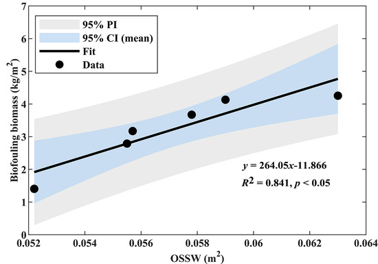
Figure 2. Process of making the panel model with a rough surface.
Jmse 14 00703 g002
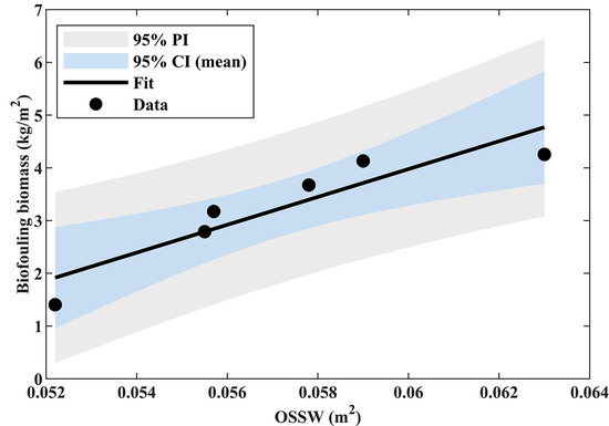
Figure 3. Deployment of the panel models in Xiangyun Bay, Tangshan, China.
Jmse 14 00703 g003


Figure 4. (a) Raw scanned point cloud of the settling plate, (b) Processed scanned point cloud of the settling plate.
Jmse 14 00703 g004
Figure 5. Computational domain and the boundary conditions.
Jmse 14 00703 g005
Figure 6. Mesh grid around the panel model by using the poly-hexcore approach.
Jmse 14 00703 g006
Figure 7. Variation of H and the biomass of the experimental and control panels throughout one year of immersion: (a) Mean biofouling height of the rough and control panels over time; (b) Biofouling biomass of the rough and control panels over time.
Jmse 14 00703 g007
Figure 8. Relationship between the biomass and the biofouling thickness H .
Jmse 14 00703 g008
Figure 9. (a) Canopy roughness R C ; (b) Surface heterogeneity σ ; and (c) Fractal dimension D of two panel types under different deployment times. Data are presented as medians with boxplots. Asterisks indicate significant differences between panel types at each time point (* p < 0.05; **   p < 0.01), and “ns” indicates no significant difference.
Jmse 14 00703 g009
Figure 10. Spearman Correlation between the canopy roughness R C and surface heterogeneity σ .
Jmse 14 00703 g010
Figure 11. The relative velocity ( u / u 0 ) distribution around the rough and control panels on the y = 0 vertical plane and z = H + 1 horizontal plane at different deployment times: (a) 0-month immersion (June 2024); (b) 6-month immersion (November 2024); (c) 12-month immersion (June 2025).
Jmse 14 00703 g011
Figure 12. Upwelling region (left side) and wake region (right side) around the rough and control panels at different deployment times: (a) 0-month immersion (June 2024); (b) 6-month immersion (November 2024); (c) 12-month immersion (June 2025).
Jmse 14 00703 g012
Figure 13. Upwelling volume and wake volume of two panel types under different deployment times: (a) Upwelling volume of the panels, Vup; (b) Normalized upwelling volume of the panels, Vup/Vpanel; (c) Wake volume of the panels, Vwake; (d) Normalized wake volume of the panels, Vwake/Vpanel.
Jmse 14 00703 g013
Figure 14. Shear stress distribution contours of the biofouling panels at different immersion times: (a) rough panels under 0-, 6-, and 12-month; (b) Control panels under 0-, 6-, and 12-month.
Jmse 14 00703 g014
Figure 15. The Optimal Shear Stress Window area of the rough and control panels at different immersion times.
Jmse 14 00703 g015
Figure 16. Distribution contours of the normalized spanwise vorticity ( ω z D / u 0 ) in the horizontal plane: (a) the rough and control panels under 0-month immersion; (b) the rough and control panels under 6-month immersion; (c) the rough and control panels under 12-month immersion.
Jmse 14 00703 g016
Figure 17. Distribution contours of the wall-normal vorticity ( ω y D / u 0 ) in the vertical plane: (a) the rough and control panels under 0-month immersion; (b) the rough and control panels under 6-month immersion; (c) the rough and control panels under 12-month immersion.
Jmse 14 00703 g017
Figure 18. Relationship between the canopy roughness R C and the OSSW area.
Jmse 14 00703 g018
Figure 19. Relationship between the OSSW area and biofouling biomass.
Jmse 14 00703 g019
Figure 20. The relative height contours of the rough panels under different immersion times: (a) 0 months; (b) 6 months; (c) 12 months.
Jmse 14 00703 g020
Figure 21. Comparison of the small-scale vortices in the near-wall region under different immersion times: (a) the rough panels and (b) the smooth control panels.
Jmse 14 00703 g021
Table 1. Increase in biofilm thickness increment ( H ) variation at different times.
Interval (Months)Biofilm Thickness (H)Biofilm Thickness (∆H)
Rough Panels
(mm)
Control Panels
(mm)
Rough Panels
(mm)
Control Panels
(mm)
0~32.7652.2992.7652.299
3~63.7573.4140.9921.115
6~94.9324.4511.1751.037
9~126.3885.9081.4551.458
Disclaimer/Publisher’s Note: The statements, opinions and data contained in all publications are solely those of the individual author(s) and contributor(s) and not of MDPI and/or the editor(s). MDPI and/or the editor(s) disclaim responsibility for any injury to people or property resulting from any ideas, methods, instructions or products referred to in the content.