Simulation-Based Evaluation of a Single-Line Laser Framework for AUV Wall-Following and Mapping

Abstract

This study presents a simulation-based evaluation of a wall-following and mapping framework for autonomous underwater vehicles (AUVs) equipped with a single-line laser, targeting structured environments such as rectangular tanks and dam interiors. A hardware-in-the-loop (HIL) simulation platform is developed to integrate sensor emulation, vehicle dynamics, and image-based control while preserving the onboard data formats, update rates, and communication protocols of the AUV system. Using a single camera–laser pair, the framework estimates yaw angle and lateral wall distance from laser image geometry to support real-time wall-following and frontal obstacle avoidance. Wall mapping is performed by transforming laser image features into spatial coordinates and estimating the dimensions of geometric protrusions. The framework is evaluated on simulated walls with protruding features under two navigation conditions: ideal-motion and dynamic-control operation. Simulation results show stable wall-following performance, with lateral distance errors typically below 0.1 m. Under ideal-motion conditions, mapping errors range from 1% to 13%, while under dynamic-control navigation they increase to 10–35% due to attitude fluctuations and control-induced motion. Frontal obstacle avoidance maintains a minimum clearance of 1.04 m. The results demonstrate the feasibility of using a single-line laser and a unified image stream for both real-time wall-following control and post-mission geometric mapping within the defined simulation conditions. While the evaluation is limited to simulation and assumes idealized optical conditions without modeling hydrodynamic disturbances or optical degradation effects, the framework provides a system-level reference for laser-guided inspection strategies in confined underwater environments such as tanks, reservoirs, and dams.

1. Introduction

Submerged structures such as dams, reservoirs, and enclosed water containment systems require periodic inspection to assess corrosion, structural degradation, and biological growth. According to the International Commission on Large Dams (ICOLD) [1], the World Register of Dams currently contains records for more than 62,000 dams worldwide, many of which require periodic inspection and maintenance throughout their service life to ensure structural safety and operational reliability. Such inspections support maintenance planning, safety assessment, and risk mitigation in engineered underwater environments where structural integrity must be monitored over long operational lifetimes.

Traditionally, underwater inspections are performed by human divers or remotely operated vehicles (ROVs). Diver-based operations involve safety risks, depth limitations, and restricted working durations, while ROV-based inspection requires tether management and skilled operators. Autonomous underwater vehicles (AUVs) provide an untethered alternative that can reduce operational complexity and improve coverage efficiency, particularly in structured underwater environments. Existing AUV inspection systems typically employ optical cameras, sonar sensors, or structured-light techniques to support navigation, structural inspection, and geometric reconstruction tasks.

However, fully autonomous inspection in open and unstructured underwater settings remains challenging due to environmental uncertainty and limited onboard perception. As a scoped and controlled investigation, this study focuses on structured near-field environments, specifically a rectangular tank representing engineered containment structures such as dam interiors or inspection chambers.

An AUV equipped with a single-line laser and monocular camera is used to investigate wall-following and surface mapping under simulated conditions. Laser-based sensing provides fine geometric resolution at short range and is therefore suitable for confined inspection scenarios where geometric features must be resolved.

The proposed framework extracts yaw deviation and lateral wall distance from laser projection images to enable closed-loop wall-following and frontal obstacle avoidance. A hardware-in-the-loop (HIL) simulation framework emulates AUV dynamics, image processing, and sensor feedback in real time. Wall mapping is achieved by transforming laser stripe features into 3D coordinates and estimating protrusion dimensions during layer-by-layer scanning.

This study evaluates the feasibility of a compact single-line laser sensing configuration for three closely related inspection capabilities: laser-based perception, closed-loop wall-following control, and geometric surface mapping. The evaluation is constructed using a hardware-in-the-loop (HIL) simulation framework that emulates vehicle dynamics, sensor feedback, and onboard computation under controlled conditions. Simulation results assess wall-following stability, mapping accuracy under ideal-motion and dynamic-control scenarios, and frontal wall avoidance performance, while acknowledging the simplified environmental assumptions adopted in this work.

Accordingly, the objective of this study is to evaluate the feasibility of a single-line laser-based perception and control framework for AUV wall-following, geometric mapping, and frontal obstacle avoidance under controlled hardware-in-the-loop simulation assumptions, rather than to provide a comprehensive environmental model of open-water inspection conditions.

2. Related Work

Several studies have investigated the integration of laser sensing technologies with autonomous underwater vehicles for structural inspection and geometric measurement. Kondo and Ura [2] presented an early laser-based inspection system combining a CCD camera with two point-lasers to maintain approximate standoff distance during infrastructure inspection. Distance and angular displacement were estimated via triangulation and lens calibration. The authors noted limitations in measurement redundancy and robustness under rough surface conditions. To improve feature continuity, Kondo et al. [3] later replaced dual point-lasers with a single-line laser, demonstrating improved tracking stability on the Tri-Dog I AUV. In related work, Kondo et al. [4] also demonstrated 3D reconstruction and real-time vehicle control using line laser sensing. Maki et al. [5,6] investigated multimodal sensor fusion for jacket-type offshore platform inspection, combining sonar for long-range detection and line laser imagery for near-field precision. Their framework incorporated map-based navigation and control, validated on the Tri-Dog I platform. Albiez et al. [7] developed a pan-tilt laser-optical inspection module for the SeaCat AUV, enabling scanning of vertical underwater surfaces. Jacobi [8] proposed a corresponding motion control strategy and demonstrated feasibility through simulation and field trials. Inzartsev et al. [9] applied line laser sensing for AUV-based pipeline tracking, showing detection and following performance in simulation.

Structured-light techniques have also been employed for high-resolution underwater 3D reconstruction. For example, the Tuna Sand AUV and the SeaXerocks system deployed on the ROV Hyper-Dolphin were used for dense 3D imaging under hydrothermal conditions [10]. Nakatani et al. [11] demonstrated a rotary laser scanning system integrated with the Tuna Sand AUV for mapping hydrothermal chimneys. Prats et al. [12] implemented manipulator-mounted laser scanning on the Girona 500 AUV for targeted reconstruction tasks. Caccia [13] developed a laser-based triangulation and optical correlation system for precise vehicle motion estimation. Hu et al. [14] proposed a structured-light 3D detection system for underwater pipelines, integrating point cloud processing and target-focused extraction strategies for fine structural inspection in energy transportation scenarios.

While these studies demonstrate the applicability of laser-based systems for local 3D reconstruction, pipeline tracking, or structure-specific inspection tasks, their primary emphasis lies in reconstruction methodologies, sensing architectures, or task-specific implementations. The interaction between wall-following control behavior and geometric mapping performance within a structured inspection scenario has received comparatively less focused discussion.

In contrast, the present study addresses a more scoped problem: integrating wall-following control, frontal obstacle detection, and geometric surface reconstruction within a structured and confined inspection scenario using a single-line laser. The objective is not to replace multi-sensor systems, but to evaluate the capability and limitations of a compact laser-based configuration under controlled simulation conditions.

A preliminary version of this work was presented at the IEEE OCEANS 2024 Halifax conference [15]. The current manuscript extends that study by introducing a hardware-in-the-loop simulation framework, providing detailed derivations of the image-based control algorithmics, and evaluating wall-following and mapping performance for walls with geometric protrusions under both ideal-motion and dynamic-control navigation, including frontal obstacle avoidance behavior.

3. Methods and Simulation Framework

Underwater structural inspections have traditionally relied on human divers or ROVs to capture imagery for post-mission analysis. This study proposes a more autonomous approach: using an AUV equipped with a single-line laser imaging system to follow walls and record elevation variations in real time. Standard onboard sensors such as gyroscopes and Doppler velocity logs (DVLs) can estimate internal state variables such as orientation and velocity, but not the AUV’s position relative to nearby structures. Acoustic sensors (e.g., single-beam, multibeam, or scanning sonars) offer robust performance in turbid conditions but generally lack the spatial resolution required for fine-scale surface inspection in confined spaces. Laser-based sensing systems, in contrast, provide fine geometric information at short range and are therefore suited for near-field inspection tasks in structured environments. Mounted on an AUV, a single-line laser and camera configuration enables estimation of the vehicle’s relative position to a wall, regulation of lateral offset, tangential heading alignment, and frontal obstacle detection within the defined sensing range. Although optical sensing is sensitive to environmental conditions and has limited operational range, it is particularly applicable to confined inspection scenarios such as tanks, dam interiors, and engineered water containment systems. In this study, optical refraction, scattering, and attenuation effects are not modeled, and the analysis assumes clear-water conditions for geometric evaluation, with idealized laser stripe visibility. The following sections describe the geometric modeling, image-based estimation algorithms, and hardware-in-the-loop simulation framework used to evaluate this near-field inspection approach under controlled simulation assumptions. Unless otherwise stated, all geometric estimations assume a planar wall, clear-water conditions, continuous laser stripe visibility, and neglect optical distortion, refraction, scattering, and attenuation effects.

3.1. AUV Platform and Single-Line Laser Configuration

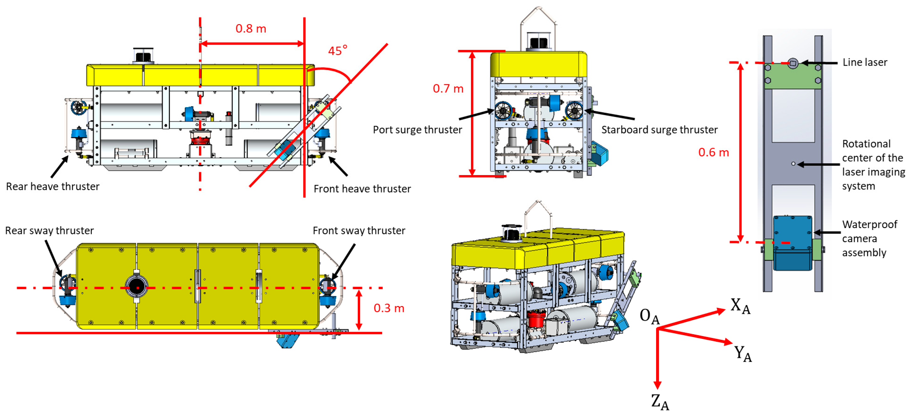
The experimental platform is the IUT AUV-I, developed by the Institute of Undersea Technology at National Sun Yat-sen University. The vehicle has a cuboid frame measuring approximately 1.88 m × 0.57 m × 0.88 m. To reduce frontal exposure to the direction of motion, the laser imaging module is installed on the starboard side—one of the longer lateral faces—rather than the bow or stern. Mounting on the bow or stern would increase the projected frontal area during forward motion and could introduce additional hydrodynamic loading effects. The sensing system consists of a single-line laser and a waterproof camera. Two projection modes were considered: vertical (stripe projected downward onto the wall) and horizontal (stripe projected forward). Vertical projection enables lateral distance estimation for wall-following control but does not provide direct frontal sensing. Horizontal projection supports frontal obstacle detection but requires vertical AUV motion for full surface coverage, increasing motion planning complexity. To combine both capabilities within a single configuration, the laser system is installed at the front-right corner of the AUV. In the body-fixed frame (${\mathrm{O}}_{\mathrm{A}}$, ${\mathrm{X}}_{\mathrm{A}}$, ${\mathrm{Y}}_{\mathrm{A}}$, ${\mathrm{Z}}_{\mathrm{A}}$), it is positioned at (0.8 m, 0.3 m, 0 m) relative to the AUV’s center of gravity (CG) and tilted 45° counterclockwise about the ${\mathrm{Y}}_{\mathrm{A}}$ axis, with the rotation angle selected to balance lateral wall visibility and forward obstacle detection within the camera field of view. The installation geometry is defined kinematically and does not include deformation, vibration, or alignment uncertainty effects. This forward-and-lateral orientation supports simultaneous wall tracking and frontal obstacle detection within the near-field inspection range considered in this study. The geometric installation layout and thruster configuration are illustrated in Figure 1.

3.2. Relative Position Estimation from Laser Imagery

The laser emitter is vertically mounted 0.6 m above the camera lens, with both components assumed to be aligned on the same plane within the simulation model. The camera’s optical axis is configured to intersect the inspection wall at a nominal distance of 1.5 m from the laser origin, resulting in an elevation angle of 21.8° in the geometric model, determined by the relative vertical offset between the laser and camera and the specified working distance.

To determine the AUV’s position relative to the inspection wall, this study adopts the Earth-fixed and body-fixed coordinate conventions described by Fossen [16]. The transformation between the Earth-fixed frame (${\mathrm{O}}_{\mathrm{E}}$, ${\mathrm{X}}_{\mathrm{E}}$, ${\mathrm{Y}}_{\mathrm{E}}$, ${\mathrm{Z}}_{\mathrm{E}}$) and the body-fixed frame (${\mathrm{O}}_{\mathrm{A}}$, ${\mathrm{X}}_{\mathrm{A}}$, ${\mathrm{Y}}_{\mathrm{A}}$, ${\mathrm{Z}}_{\mathrm{A}}$) is represented using a rotation matrix $R\left({\mathrm{\varnothing }}_A,{\theta }_A,{\psi }_A\right)$ that incorporates the AUV’s roll (${\mathrm{\varnothing }}_A$), pitch (${\theta }_A$), and yaw (${\psi }_A$) angles, as defined in Equation (1):

$$\left[\begin{array}{c}{\mathrm{X}}_{\mathrm{E}}\\ {\mathrm{Y}}_{\mathrm{E}}\\ {\mathrm{Z}}_{\mathrm{E}}\end{array}\right]=R\left({\mathrm{\varnothing }}_A,{\theta }_A,{\psi }_A\right)\left[\begin{array}{c}{\mathrm{X}}_{\mathrm{A}}\\ {\mathrm{Y}}_{\mathrm{A}}\\ {\mathrm{Z}}_{\mathrm{A}}\end{array}\right]$$

(1)

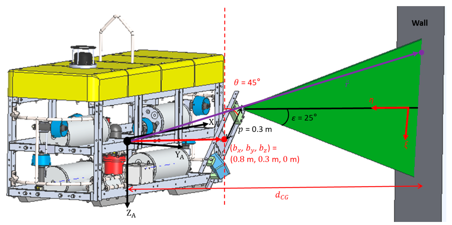
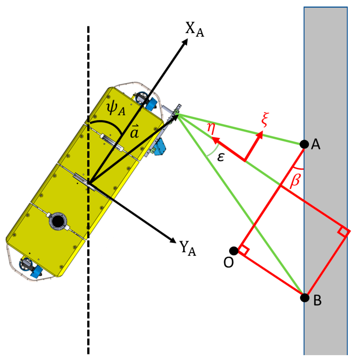
The relative geometry between the AUV, laser imaging module, and the wall surface is shown in Figure 2. The vector $(b_x,b_y,b_z)$ denotes the laser module’s position in the body-fixed frame, and $(r_x,r_y,r_z)$ represents the coordinates of a laser-illuminated point on the inspection surface. A geometric expression for this position vector $\stackrel{⃑}{r}=(r_x,r_y,r_z)$ is formulated based on the laser projection model implemented in the OpenGL (version 4.6)-based simulated environment under the previously defined assumptions.

A two-step coordinate transformation is used to convert pixel coordinates from laser images to physical coordinates on the inspection surface. In Step 1, the pixel coordinates ($\tilde{i}$, $\tilde{j}$) are mapped to near clipping plane coordinates ($\tilde{x}$, $\tilde{y}$). The image dimensions are $m\times n$, with vertical field of view $2\omega$ and distance h from the camera to the near clipping plane, where $m$ and $n$ denote the horizontal and vertical pixel resolutions, respectively. Assuming ideal pinhole projection and neglecting optical distortion and refraction effects within the simulation environment, this mapping is defined in Equation (2):

$$\left\{\begin{array}{c}\tilde{i}={\displaystyle \frac{\frac{n\tilde{x}}{h}}{2\tan \omega }}+{\displaystyle \frac{m}{2}}\\ \tilde{j}={\displaystyle \frac{\frac{n\tilde{y}}{h}}{2\tan \omega }}+{\displaystyle \frac{n}{2}}\end{array}\right.$$

(2)

In Step 2, the normalized coordinates ($\tilde{x}$, $\tilde{y}$) are mapped to coordinates ($\xi$, $\eta$) on the laser projection plane. Using known positions of the camera (${\xi }_c$, ${\eta }_c$, ${\zeta }_c$), the laser emitter (${\xi }_l$, ${\eta }_l$, 0), and the camera-laser elevation angle ${\theta }_c$, the transformation is defined in Equation (3):

$$\left\{\begin{array}{c}{\displaystyle \frac{\tilde{x}}{h}}={\displaystyle \frac{\xi }{{\zeta }_c\sin {\theta }_c+(\eta -{\eta }_c)\cos {\theta }_c}}\\ {\displaystyle \frac{\tilde{y}}{h}}={\displaystyle \frac{{\zeta }_c\cos {\theta }_c-(\eta -{\eta }_c)\sin {\theta }_c}{{\zeta }_c\sin {\theta }_c+(\eta -{\eta }_c)\cos {\theta }_c}}\end{array}\right.$$

(3)

Combining the two steps provides the transformation from pixel coordinates ($\tilde{i}$, $\tilde{j}$) to laser-plane coordinates ($\xi$, $\eta$) within the defined geometric assumptions, as shown in Equation (4):

$$\left\{\begin{array}{c}\xi ={\displaystyle \frac{\left(2\tilde{i}-m\right)\left(\tan \omega \right)\left[{\zeta }_c\sin {\theta }_c+\left(\eta -{\eta }_c\right)\cos {\theta }_c\right]}{n}}\\ \eta ={\eta }_c+{\zeta }_c\left[{\displaystyle \frac{n\cos {\theta }_c-\left(\tan \omega \right)\left(2\tilde{j}-n\right)\left(\sin {\theta }_c\right)}{n\sin {\theta }_c+\left(\tan \omega \right)\left(2\tilde{j}-n\right)\left(\cos {\theta }_c\right)}}\right]\end{array}\right.$$

(4)

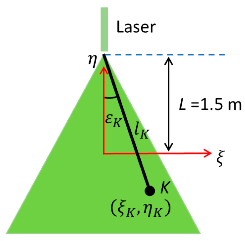
Using these coordinates, the vector from the laser emitter to a given point $K({\xi }_K,{\eta }_K)$ is characterized by its geometric length $l_K$ and angle ${\epsilon }_K$, defined in Figure 3 and computed in Equations (5) and (6):

$$l_K=\sqrt{{\xi }_K^2+{\left(L-{\eta }_K\right)}^2}$$

(5)

$${\epsilon }_K={\tan }^{-1}\left({\displaystyle \frac{{\xi }_K}{L-{\eta }_K}}\right)$$

(6)

where $L=1.5\hspace{0.17em}\mathrm{m}$ is the fixed distance between the laser emitter and the $\xi$-axis, corresponding to the nominal working distance defined in the imaging configuration.

The 3D position of the laser point in the AUV’s body-fixed frame is estimated geometrically by Equation (7):

$$\stackrel{⃑}{r}=\left(b_x+p\sin \theta +l\cos \theta \sin \epsilon ,b_y+l\cos \epsilon ,b_z+p\cos \theta -l\sin \theta \sin \epsilon \right)$$

(7)

where $p$ is the vertical offset between the laser emitter and its rotation center, and $\theta$ is the downward tilt of the laser plane as defined by the installation configuration in Section 3.1.

If the AUV is misaligned with the inspection wall under planar wall assumptions, the laser stripe appears tilted in the image. This tilt, illustrated in Figure 4, is characterized by angle $\beta$ extracted from the laser stripe orientation, and yaw deviation ${\psi }_A$ is estimated geometrically using Equation (8):

$${\psi }_A={\mathrm{t}\mathrm{a}\mathrm{n}}^{-1}\left({\displaystyle \frac{\tan \beta }{\cos \theta }}\right)$$

(8)

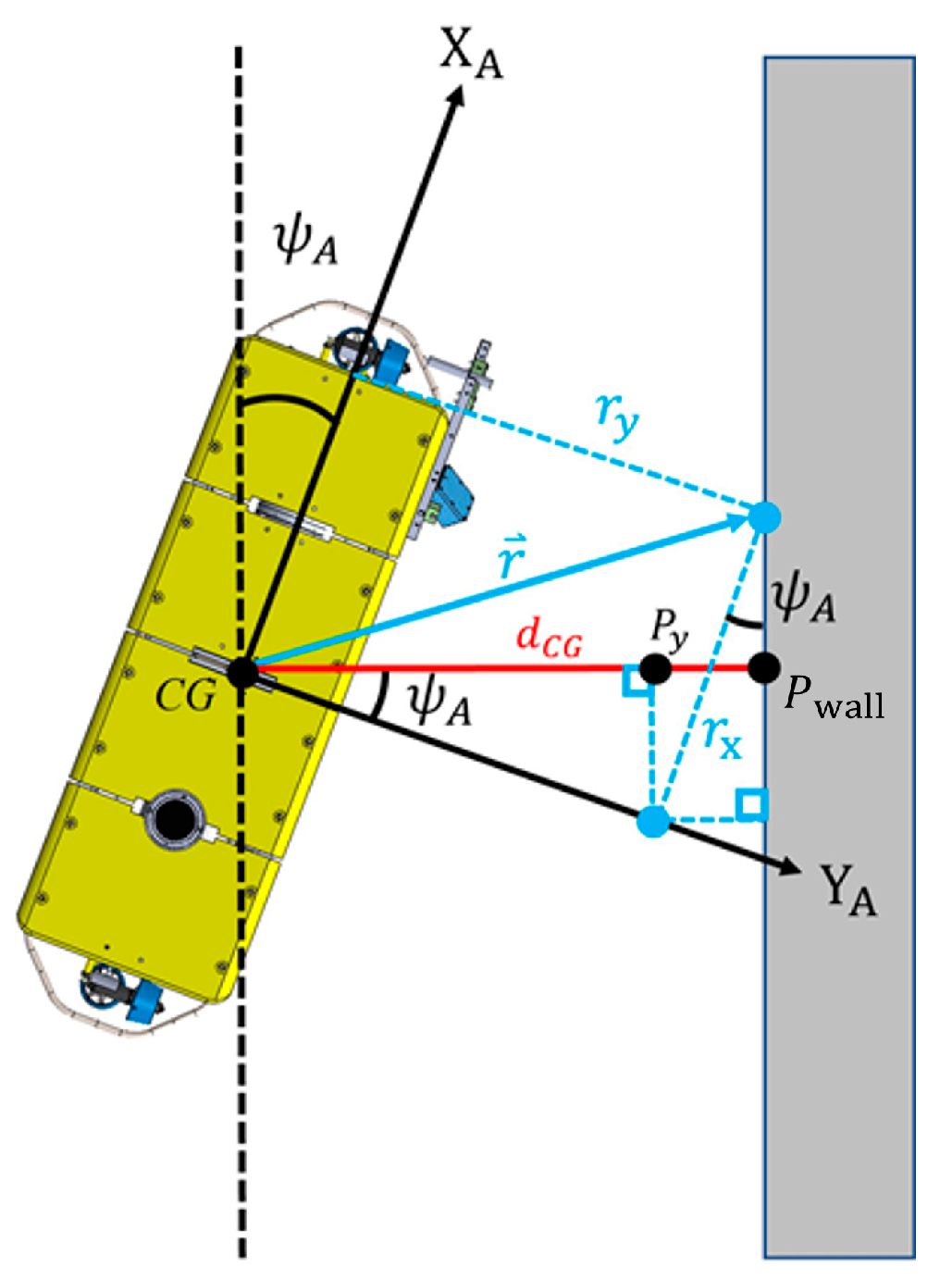
Finally, the lateral distance $d_{CG}$ from the AUV’s CG to the wall is obtained geometrically by projecting the laser point vector $\stackrel{⃑}{r}$ onto the wall normal direction under planar wall assumptions, as shown in Figure 5 and defined in Equation (9):

$$d_{\mathit{CG}}=r_x\sin {\psi }_A+r_y\cos {\psi }_A$$

(9)

3.3. Front-Side and Rear-Side Distance Estimation for Wall-Following

To maintain effective wall-following behavior, the AUV is required to remain approximately parallel to and equidistant from the inspection wall within the control objectives defined in this study. This behavior is regulated using side-mounted thrusters located at the front and rear of the vehicle, independently actuated based on geometric distance feedback within the simulation model.

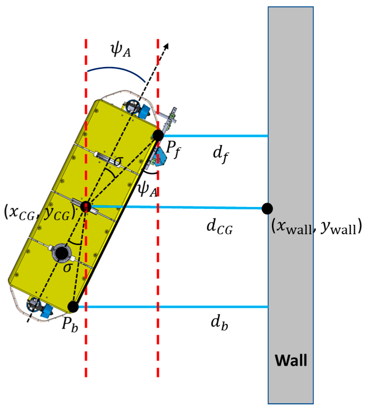
Two key geometric measurements are used in the wall-following control logic: the distance from the AUV’s front-right corner to the wall, denoted $d_f$, and the distance from the rear-right corner to the wall, denoted $d_b$. These distances are computed geometrically from the lateral CG distance $d_{CG}$ defined in Equation (9) and the assumed rigid-body vehicle geometry defined in Section 3.1, as illustrated in Figure 6. The distances are computed using Equations (10) and (11):

$$d_f=d_{CG}-\overline{CG{P}_f}\sin \left(\sigma +{\psi }_A\right)$$

(10)

$$d_b=d_f+\overline{P_f{P}_b}\sin \left({\psi }_A\right)$$

(11)

where $\overline{CG{P}_f}=\sqrt{{0.3}^2+{0.8}^2}\approx 0.854 \mathrm{m}$ represents the nominal distance from the AUV center of gravity to the front-right corner based on the installation geometry defined in Section 3.1; $\overline{P_f{P}_b}=1.6 \mathrm{m}$ represents the nominal longitudinal separation between the front and rear reference corners; $\sigma ={\tan }^{-1}\left({\displaystyle \frac{0.3}{0.8}}\right)\approx 20.6°$ represents the geometric angle between the vehicle longitudinal axis and the vector from the CG to the front-right corner. These expressions provide geometric distance references for front and rear lateral control under the simulated planar wall-following configuration.

3.4. Frontal Distance Estimation for Collision Avoidance

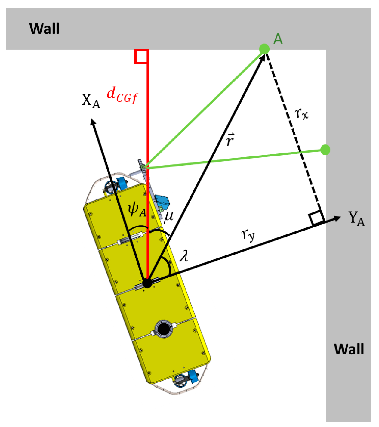
To support frontal collision avoidance, the AUV estimates the distance $d_{CGf}$ from its CG to the wall directly ahead within the geometric framework defined in this study. The AUV’s initial heading is defined as true north (${\psi }_A=0°$). When the AUV approaches the wall with a yaw deviation ${\psi }_A$, the leftmost point A on the simulated laser stripe projected onto the wall is identified under the assumption of continuous and fully visible laser stripe projection, and its position vector $\stackrel{⃑}{r}$ is decomposed into components $r_x$ and $r_y$, as illustrated in Figure 7.

The intermediate angle $\lambda ={\tan }^{-1}\left({\displaystyle \frac{r_y}{r_x}}\right)$ is computed from the projected point geometry under the planar wall assumption. The angular offset $\mu$ between the AUV heading and point A is then defined geometrically as Equation (12):

$$\mu =\left\{\begin{array}{c}{90}^{°}-{\psi }_A-\lambda ,{ \psi }_A<0\\ {90}^{°}+{\psi }_A-\lambda ,{\psi }_A>0\end{array}\right.$$

(12)

The frontal distance $d_{CGf}$ is estimated geometrically by projecting the vector magnitude onto the forward direction as shown in Equation (13):

$$d_{CGf}=\sqrt{r_x^2+r_y^2}\cos \left(\mu \right)$$

(13)

These expressions provide a geometric estimate of frontal distance under the assumption of a locally planar wall, continuous laser stripe visibility, and idealized optical projection (i.e., without refraction, scattering, or attenuation effects) within the camera field of view.

3.5. Laser Stripe Extraction via Brightness Centroid Estimation

To support simulation development, a real-world laser image captured in air was analyzed to obtain a qualitative reference for the geometric and radiometric properties of the projected laser stripe. Although air and water differ optically, and underwater scattering and attenuation are not modeled in this study, the image was used as a qualitative reference for validating the simulated stripe profile under controlled conditions. Each pixel encodes RGB intensity values (0~255), with the peak intensity near the stripe center and gradual falloff toward the edges. The green channel intensity distribution was approximated from the reference image to generate simulated stripe profiles under controlled rendering conditions.

Stripe extraction in simulation employs threshold-based binarization on the green channel, with a fixed threshold value of 230 used to isolate high-intensity pixels, selected empirically to ensure consistent stripe extraction under the defined simulation conditions. For each image column, the number of pixels exceeding the threshold is denoted by n. In real-world reference images, the stripe typically spans 8~10 pixels per column, whereas in simulation it spans 6~8 pixels, indicating approximate geometric similarity under the adopted rendering conditions.

To obtain subpixel-level geometric estimation within the simulation, the brightness centroid method [17] is applied column-wise. The subpixel vertical coordinate $Y_p$ of the stripe center is computed using Equation (14):

$$Y_p={\displaystyle \frac{{\sum }_{i=1}^n{I}_i{y}_{p_i}}{{\sum }_{i=1}^n{I}_i}}$$

(14)

where $I_i$ denotes the intensity of the i-th pixel and $y_{p_i}$ its vertical coordinate. Repeating this process across relevant columns yields a subpixel-resolved laser stripe contour for subsequent geometric estimation under the defined image assumptions.

The threshold value and intensity model are selected for the simulated environment based on the above empirical observations and are not optimized for varying turbidity, scattering, attenuation, or sensor noise conditions; robustness under such effects is beyond the scope of this study.

3.6. Mode Switching Between Wall-Following and Obstacle Avoidance

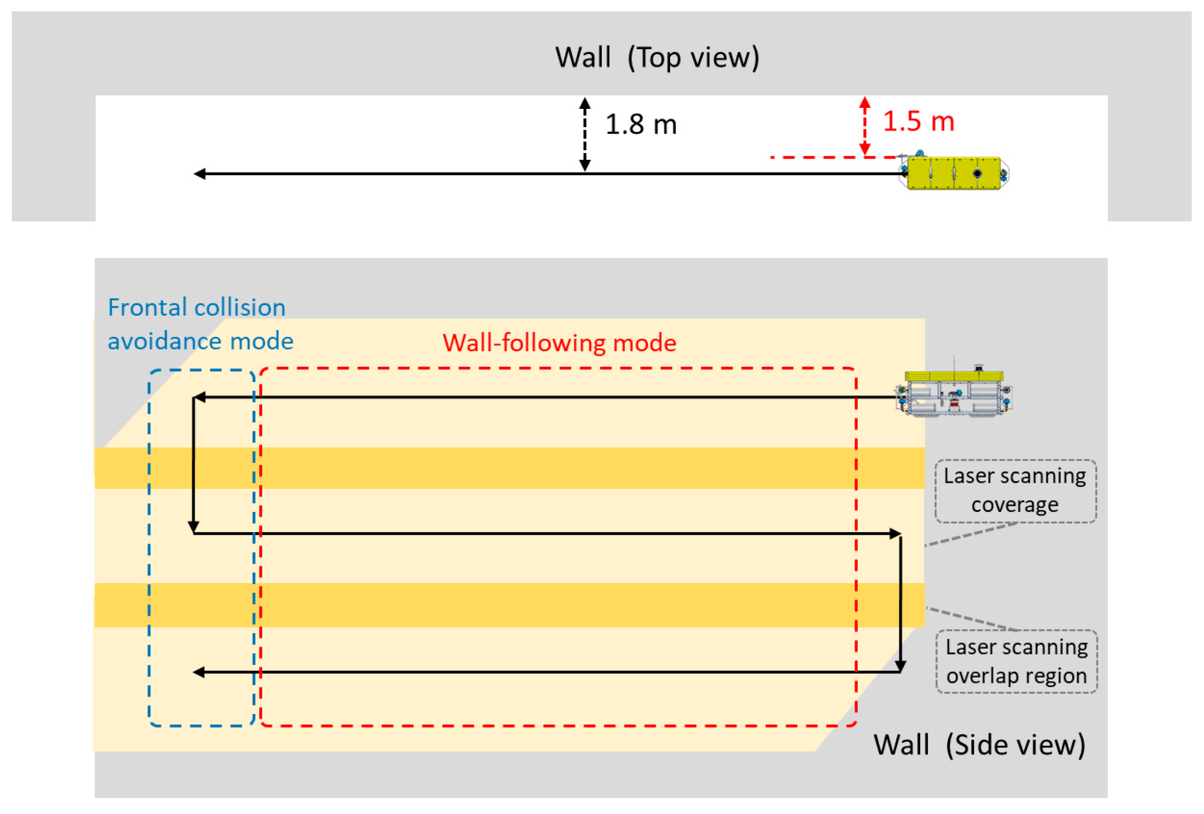
This study simulates AUV operations in a rectangular tank, where wall-following is performed at fixed depths, as shown in Figure 8. The AUV maintains a lateral offset of 1.5 m from the right-side wall (1.8 m from its CG) and scans the wall surface layer by layer. Upon detecting a frontal wall, the AUV halts, adjusts depth, and resumes motion parallel to the wall to promote full surface coverage under the defined scanning strategy. This scanning strategy is defined specifically for structured rectangular geometries and assumes orthogonal wall intersections.

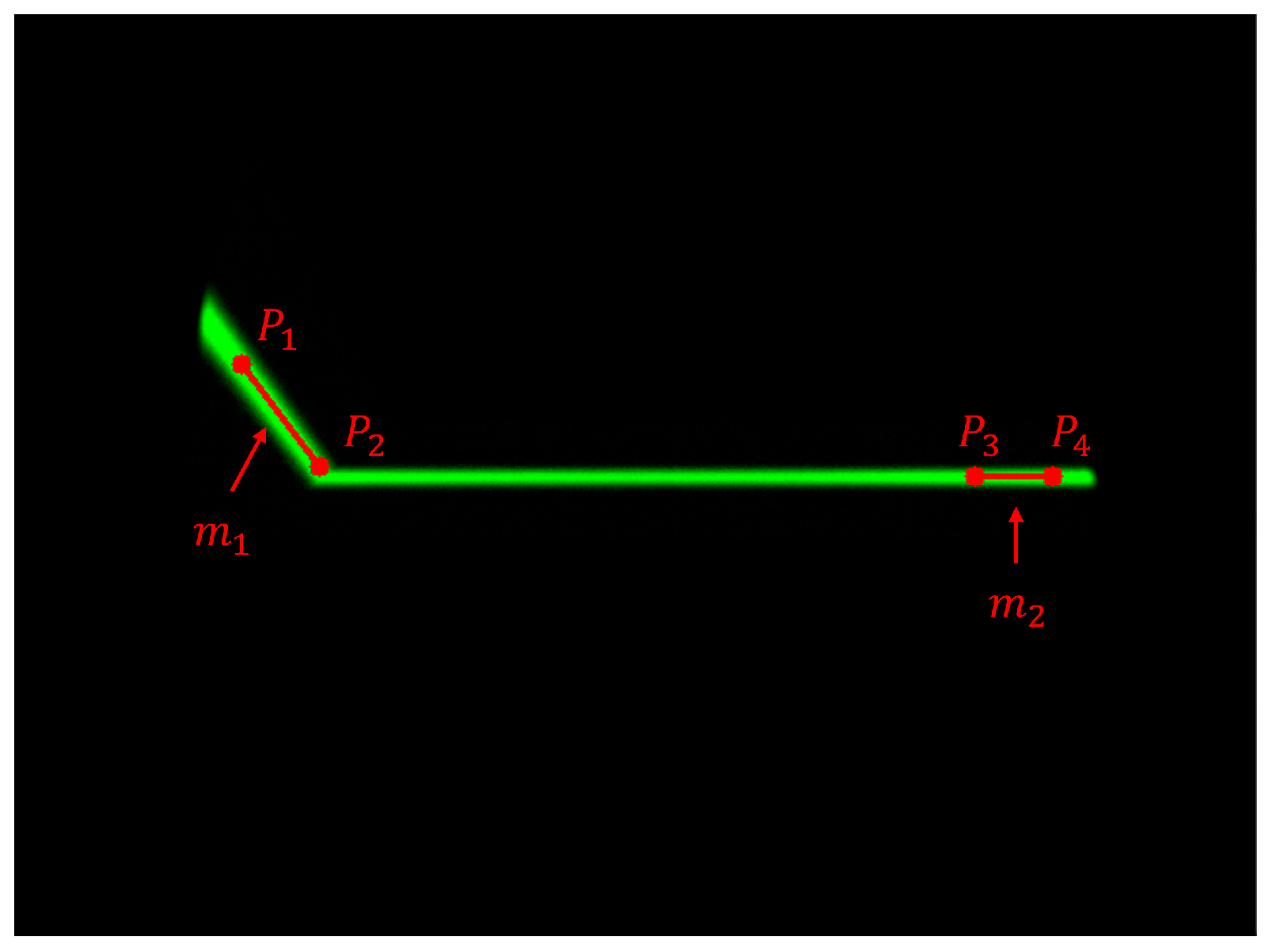
Although only a front-right laser imaging module is used, complete wall sensing coverage would generally require an additional rear-mounted module. To enable autonomous switching between wall-following and frontal avoidance modes, the AUV analyzes the geometric characteristics of the detected laser stripe, as illustrated in Figure 9.

Four stripe points are selected based on fixed pixel offsets from the detected stripe boundaries: (1) on the left, points $P_1$ and $P_2$ are extracted from 20 and 60 pixels to the right of the leftmost stripe column; (2) on the right, points $P_3$ and $P_4$ are extracted from 60 and 20 pixels to the left of the rightmost stripe column. All points are transformed into the laser projection plane. The slopes $m_1$ (between $P_1$ and $P_2$) and $m_2$ (between $P_3$ and $P_4$) are used to approximate the tangent directions of the frontal and side walls under planar wall assumptions. The angular difference, denoted as ${\theta }_{\mathrm{A}\mathrm{n}\mathrm{g}\mathrm{l}\mathrm{e}}$, is calculated using Equation (15):

$${\theta }_{\mathrm{A}\mathrm{n}\mathrm{g}\mathrm{l}\mathrm{e}}={\tan }^{-1}\left({\displaystyle \frac{m_1-m_2}{1+m_1{m}_2}}\right)$$

(15)

Table 1. Geometrically computed angle between frontal and side walls under different yaw orientations within the assumed perpendicular wall configuration.

${\mathit{\psi }}_{\mathit{A}}$	${\mathit{\theta }}_{\mathbf{A}\mathbf{n}\mathbf{g}\mathbf{l}\mathbf{e}}$
0°	88.2°
3°	−90.4°
6°	−96°
9°	−97.7°
−3°	88.7°
−6°	90.1°
−9°	90.6°

summarizes the geometrically computed ${\theta }_{\mathrm{A}\mathrm{n}\mathrm{g}\mathrm{l}\mathrm{e}}$ values under various yaw angles ${\psi }_A$ within the assumed perpendicular wall geometry.

Mode switching is triggered when $\left|{\theta }_{\mathrm{A}\mathrm{n}\mathrm{g}\mathrm{l}\mathrm{e}}\right|$ falls between 80° and 100°, indicating the likely presence of a frontal wall under the assumed orthogonal wall configuration and the current image resolution. Otherwise, the wall-following mode remains active within the defined control logic. The switching threshold is empirically determined based on simulation observations under the defined geometric and imaging conditions and should not be interpreted as a universal parameter for arbitrary wall geometries.

Preliminary simulation tests informed the choice of point spacing. A spacing of 30 pixels yielded ${\theta }_{\mathrm{A}\mathrm{n}\mathrm{g}\mathrm{l}\mathrm{e}}=81.8°$, which in simulation increased the likelihood of false-positive switching under the defined thresholds. At 50 pixels, the value decreased to $53.2°$, reducing the sensitivity of frontal wall detection under the selected switching rule. A spacing of 40 pixels resulted in ${\theta }_{\mathrm{A}\mathrm{n}\mathrm{g}\mathrm{l}\mathrm{e}}=68.3°$, which provided a practical trade-off between switching stability (false-positive suppression) and responsiveness (detection sensitivity) within the simulation environment, and was therefore adopted. This spacing selection depends on image resolution, stripe width, and the adopted thresholding conditions under the current simulation settings.

3.7. Wall Orientation Estimation Using Probabilistic Hough Transform

To estimate the wall orientation from the laser stripe, this study adopts the probabilistic Hough transform (PHT), which modifies the classical Hough method by randomly sampling edge points to reduce computational cost while maintaining geometric consistency under the defined image conditions [18]. Each sampled edge point $(x,y)$ is mapped to the parameter space $\left(\rho ,\theta \right)$ according to Equation (16):

$$\rho =x\cos \theta +y\sin \theta$$

(16)

During wall-following, surface irregularities such as geometric protrusions may locally distort the observed stripe and introduce fragmented edge segments. To enhance tolerance to local stripe distortions within the simulation environment, PHT detects multiple candidate line segments from sampled edge points rather than enforcing a single global fit. The endpoints of the detected segments are then passed to a least-squares fitting algorithm to generate a smoothed estimate of the global wall orientation. The fitted line parameters are provided to the control loop for yaw correction and lateral offset estimation within the simulation framework.

PHT is configured with a $\rho$ resolution of 1 pixel, a $\theta$ discretization step of 1°, and a voting threshold of 50, defined with respect to the current simulation image resolution and edge density. These parameters were selected through preliminary simulation trials for the current image resolution and stripe characteristics in the structured tank simulation. The configuration provides a practical trade-off between computational efficiency (reduced sampling and voting cost) and orientation consistency (robustness to fragmented stripe segments) under the assumed near-planar wall geometry.

4. Simulation Results and Mapping Performance

4.1. Hardware-in-the-Loop Simulation Setup

The hardware-in-the-loop (HIL) simulation system extends prior work [19] with added modules for wall-following, including 3D visualization and laser image processing. The framework is designed to emulate the onboard control architecture and sensing pipeline under controlled simulation conditions and does not attempt to replicate full hydrodynamic field behavior, including turbulence, boundary-layer interactions, and flow-induced disturbances.

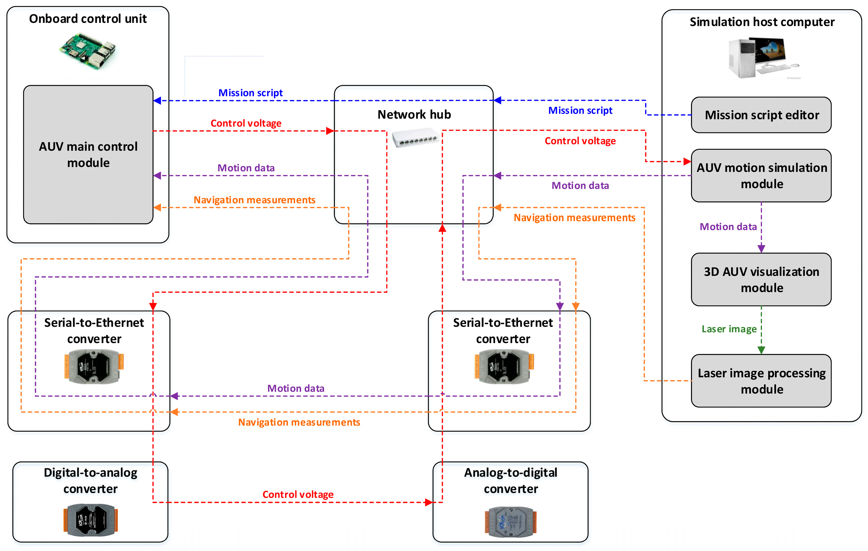
As shown in Figure 10, the platform connects a simulation host computer and the IUT AUV-I’s onboard controller (Raspberry Pi) over a network via two serial-to-Ethernet converters, supporting real-time closed-loop control within the simulation environment. The system comprises five main modules:

(1)

Mission script editor:

A GUI for configuring and uploading mission parameters.

(2)

AUV motion simulation module:

Simulates AUV dynamics using Runge–Kutta integration. Control voltages are mapped to thrusts based on empirical actuator characterization data, producing simulated velocity, orientation, and position, formatted as sensor-like outputs. The motion model includes deterministic vehicle dynamics but does not incorporate environmental disturbances such as flow-induced forces, wall-induced hydrodynamic effects, actuator nonlinearities, or time-varying disturbances.

(3)

3D AUV visualization module:

OpenGL (version 4.6) is used to render motion and generate synthetic camera views of the laser under idealized optical projection assumptions consistent with Section 3 (i.e., without refraction, scattering, or attenuation effects).

(4)

Laser image processing module:

Implemented in OpenCV (version 4.2.0), it processes 640 × 480 images at 4 FPS within the current simulation configuration to estimate yaw angle and lateral and frontal distances, and to determine the navigation mode. Outputs are sent to the controller; images and centroid positions are logged.

(5)

AUV main control module:

Computes thruster voltages from motion states and image-derived measurements. Signals pass through serial-to-Ethernet and digital-to-analog converters for actuation emulation within the HIL setup, then are re-digitized and fed back to the simulation module.

The HIL framework therefore evaluates the internal consistency of perception, control logic, and mapping algorithms within a closed-loop architecture under controlled simulation assumptions, while recognizing that full-field environmental, optical, and hydrodynamic effects are beyond the present simulation scope.

Figure 10. System architecture of the hardware-in-the-loop simulation framework under controlled modeling assumptions.

Figure 10. System architecture of the hardware-in-the-loop simulation framework under controlled modeling assumptions.

4.2. Wall-Following and Mapping with Protruding Objects

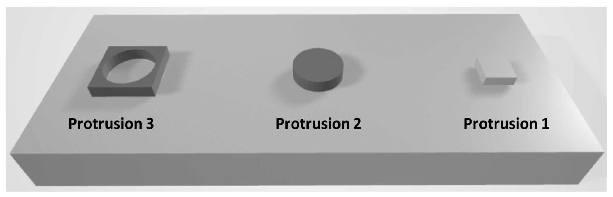
To assess the wall-following and mapping algorithm under controlled geometric discontinuities within the simulation environment, this scenario introduces three geometrically distinct protrusions on the inspection wall, as shown in Figure 11.

The objectives are twofold: (1) to examine whether the AUV maintains an approximately parallel trajectory along a wall with surface discontinuities under the defined control logic, and (2) to assess whether the single-line laser-based mapping algorithm captures the contours of these protrusions under the assumed simulation conditions.

At a nominal lateral offset of 1.5 m from the wall, the projected laser stripe spans approximately 1 m vertically under ideal geometric alignment within the simulation model (i.e., under the assumption of planar wall geometry and idealized optical projection defined in Section 3). A steady-state heave control deviation of approximately 0.1 m is incorporated in the simulation as a bounded perturbation to maintain the protrusions within the nominal sensing range under the defined conditions.

The three protrusions are:

• Protrusion 1: Cube, 0.3 m wide, 0.15 m depth.
• Protrusion 2: Cylinder, 0.5 m diameter, 0.2 m depth.
• Protrusion 3: Cube, 0.6 m wide, 0.2 m depth, with a 0.5 m centered circular hole.

Protrusion 1 is used to examine edge and corner representation in the reconstructed mapping. Protrusion 2 is used to examine curvature reconstruction characteristics under the simulation conditions. Protrusion 3 is used to assess elevation mapping behavior on a compound surface within the geometric modeling assumptions.

4.2.1. Wall-Following Control Performance

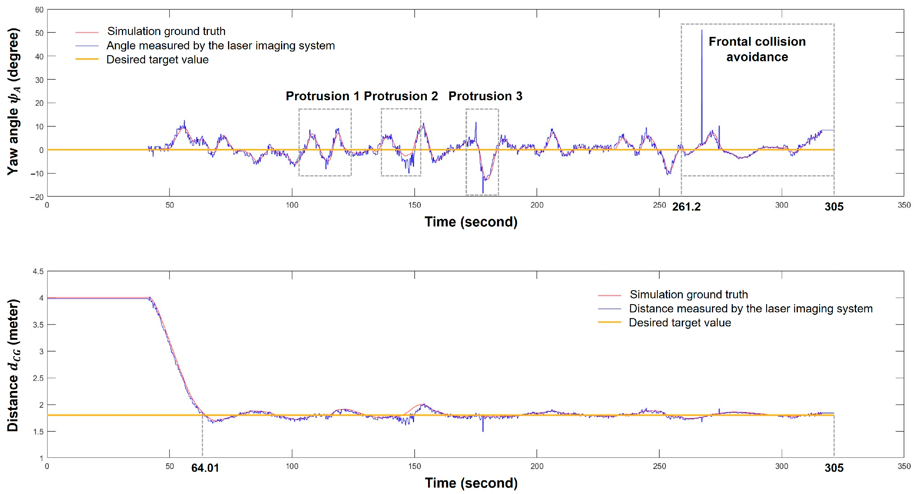
This simulation scenario examines the AUV’s wall-following behavior in the presence of three geometric protrusions while attempting to maintain a parallel and approximately constant offset from the inspection wall under the defined control logic. The control objective is to keep the starboard side of the AUV (front-right and rear-right ends) 1.5 m from the wall, corresponding to a desired CG-to-wall distance of 1.8 m.

The AUV converged to the nominal target offset at t = 64.01 s within the simulation, and the mission ended at t = 305 s, yielding an analysis window of approximately 241 s. Around t = 261.2 s, the frontal wall entered the laser image, triggering a transition to frontal avoidance mode according to the predefined switching rule.

Table 2. Errors in yaw and perpendicular distance: laser imaging vs. simulation ground truth.

Parameter	Mean Error	Standard Deviation
Yaw angle error	1.04°	4.79°
Perpendicular distance error	0.02 m	0.05 m

compares yaw angle and CG-to-wall distance between laser-derived measurements and simulation ground truth (obtained via Runge–Kutta integration of the motion model). The mean yaw deviation relative to the simulated ground truth is 1.04°, and the mean perpendicular distance deviation is 0.02 m over the analyzed interval.

Table 3. Errors in yaw and distance to wall: laser imaging vs. target values.

Parameter	Mean Error	Standard Deviation
Yaw angle error	0.11°	3.94°
Perpendicular distance error	0.01 m	0.058 m
Front-right distance error	–0.01 m	0.065 m
Rear-right distance error	–0.02 m	0.094 m

compares laser-derived measurements with predefined desired target values: 0° for yaw, 1.8 m for CG-to-wall, and 1.5 m for both front-right and rear-right distances. The maximum mean deviation among the distance measurements is 0.02 m, with standard deviations below 0.1 m in the simulation scenario.

Figure 12 compares the yaw angle ${\psi }_A$ and perpendicular distance $d_{CG}$ derived from laser imagery (blue) with simulation ground truth (red). Target values are shown in yellow (0° for ${\psi }_A$, 1.8 m for $d_{CG}$). The laser-based estimates exhibit higher variability than the simulated ground-truth signals, primarily due to the 4 Hz processing rate and geometric fluctuations of the projected stripe in the simulated environment. The yaw angle ${\psi }_A$ is computed by fitting a line to the extracted stripe, obtaining its orientation $\beta$, and mapping it to ${\psi }_A$. When this stripe geometry changes abruptly—such as during traversal of Protrusion 3 or near wall transitions—localized deviations in ${\psi }_A$ contribute to fluctuations in $d_{CG}$ within the geometric estimation model.

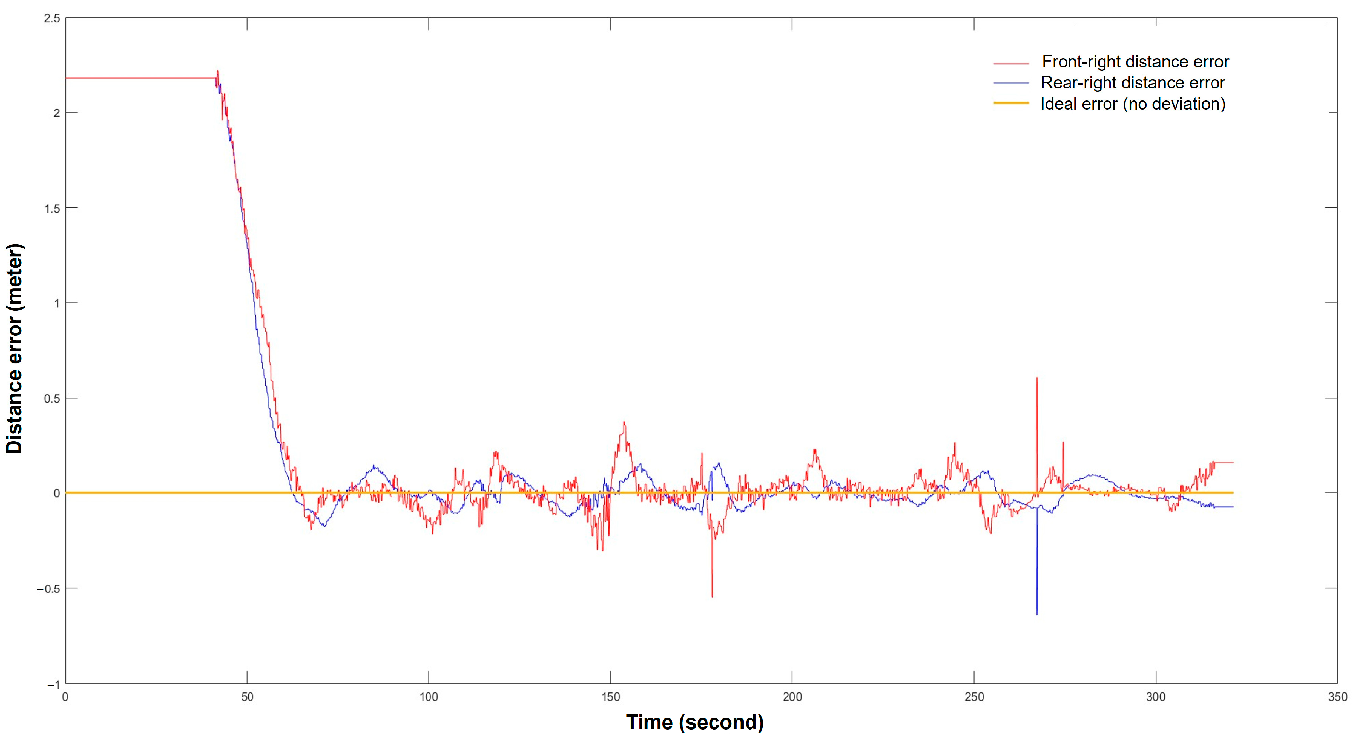
Figure 13 shows the errors in the estimated front-right distance $d_f$ and rear-right distance $d_b$ relative to the 1.5 m target. Both quantities are computed from the estimated yaw angle ${\psi }_A$ and perpendicular distance $d_{CG}$. Sudden variations in these inputs—such as when the stripe simultaneously intersects side and front surfaces or crosses protrusion boundaries—are associated with transient spikes in the distance error profiles within the simulation.

4.2.2. Wall Mapping and Protrusion Dimension Estimation

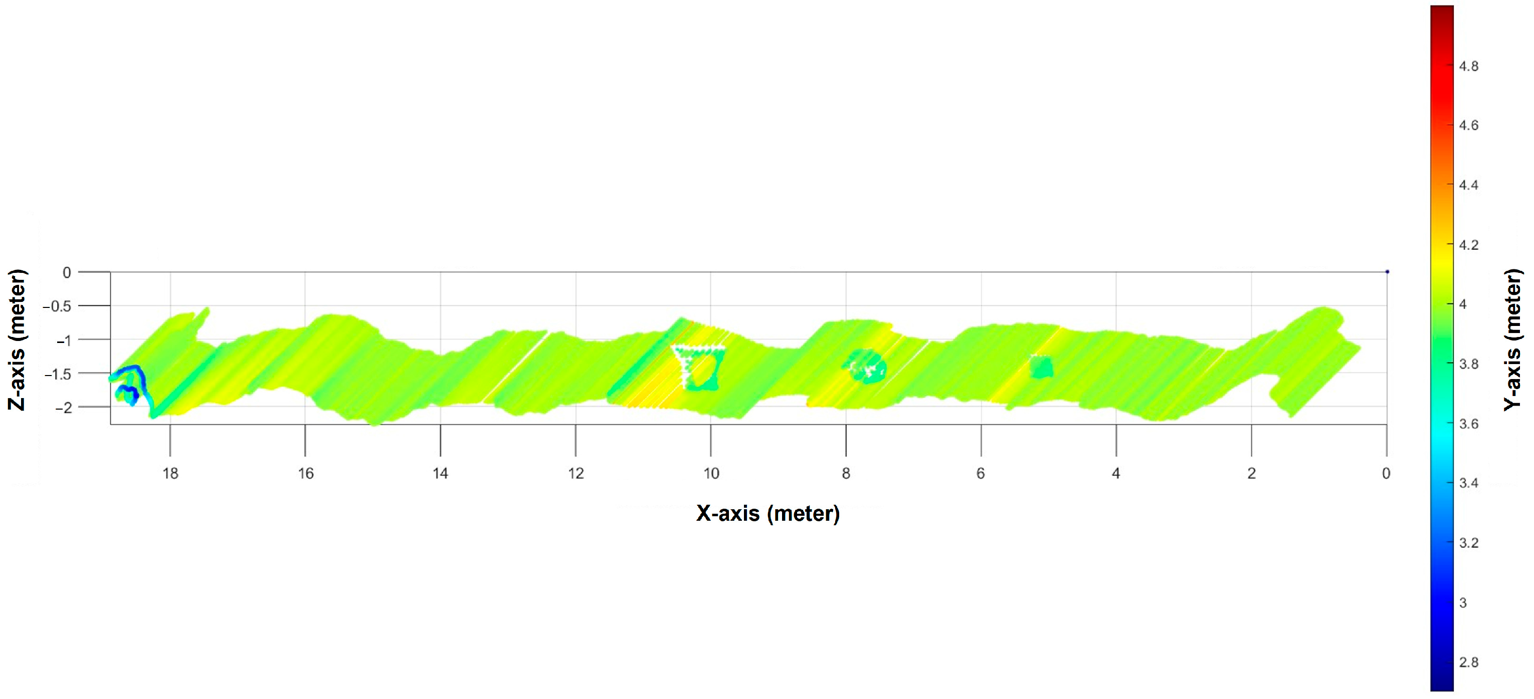
Figure 14 presents the simulated wall elevation mapping results using fused outputs from the gyrocompass, DVL, depth sensor, and laser imaging system. These data are transformed into a unified frame to generate a reconstructed wall profile under the simulated sensor and motion conditions defined in Section 4.1.

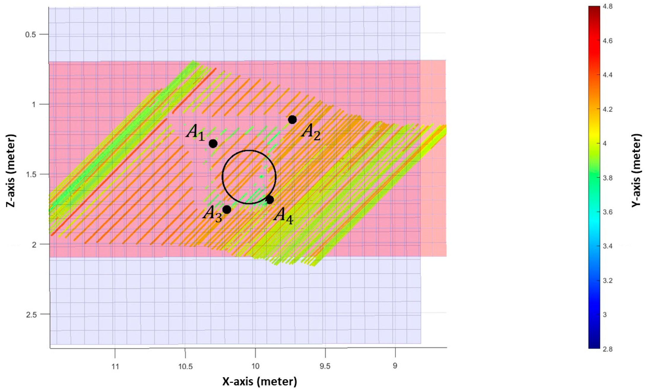
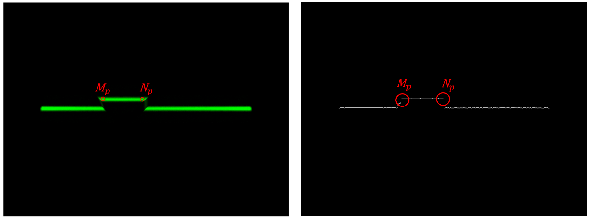
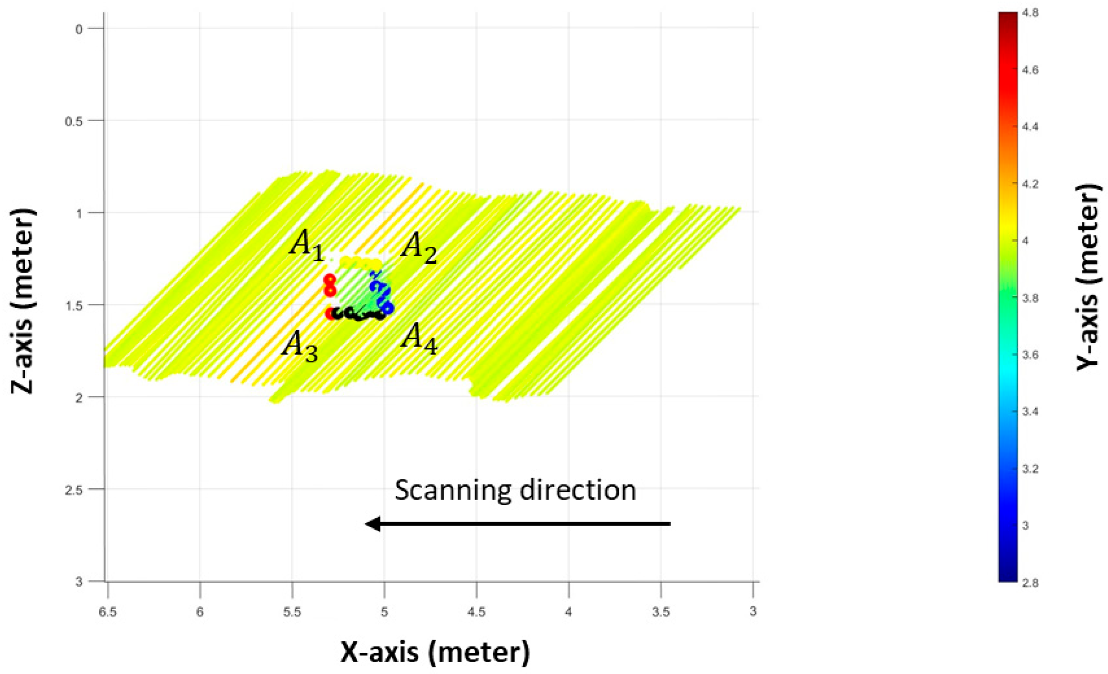
The three protrusions are individually analyzed to examine mapping behavior in two aspects: (1) protrusion height estimation and (2) geometric dimension estimation (length, width, radius) within the simulation framework. To extract boundary features, laser images (Figure 15, left) are first enhanced using the brightness centroid method described in Section 3.5. From these processed images (Figure 15, right), edge points $M_P$ and $N_P$ are selected. The vertical coordinate of the selected pixel and the column coordinate of the brightness centroid determine each boundary point in image space, which is then transformed to 3D coordinates via the geometric procedure defined in Section 3.2.

For rectangular protrusions, the longest span between edge points $M_P$ and $N_P$ is used to approximate a central dividing line. Points from images before this line are grouped into regions $A_3/A_4\left(M_P\right)$ and $A_2/A_4\left(N_P\right)$; those after the line are grouped into $A_1/A_3\left(M_P\right)$ and $A_1/A_2\left(N_P\right)$, forming the four regions in Figure 16 used for dimensional estimation under planar surface assumptions.

(1)

Plane fitting using least squares

To estimate protrusion heights, two planes are fitted to 3D points: one approximating the protrusion surface and the other approximating the surrounding wall surface. For $N$ spatial points $(x_i,y_i,z_i)$, the fitted plane $\Pi$ is expressed as Equation (17):

$$\Pi :z=Ax+By+C$$

(17)

where $A$, $B$, and $C$ are coefficients to be estimated. The squared vertical residuals are minimized via the cost function defined in Equation (18):

$$\underset{A,B,C}{\min }E\left(A,B,C\right)=\sum _{i=1}^N{(z_i-(A{x}_i+B{y}_i+C\left)\right)}^2$$

(18)

Solving the associated normal equations provides estimates of the coefficients $A$, $B$, and $C$ as given in Equation (19):

$$\left[\begin{array}{c}A\\ B\\ C\end{array}\right]={\left[\begin{array}{ccc}{\sum }_{i=1}^N{x}_i^2& {\sum }_{i=1}^N{x}_i{y}_i& {\sum }_{i=1}^N{x}_i\\ {\sum }_{i=1}^N{x}_i{y}_i& {\sum }_{i=1}^N{y}_i^2& {\sum }_{i=1}^N{y}_i\\ {\sum }_{i=1}^N{x}_i& {\sum }_{i=1}^N{y}_i& N\end{array}\right]}^{-1}\left[\begin{array}{c}{\sum }_{i=1}^N{x}_i{z}_i\\ {\sum }_{i=1}^N{y}_i{z}_i\\ {\sum }_{i=1}^N{z}_i\end{array}\right]$$

(19)

(2)

3D line fitting using least squares

To approximate protrusion edge directions, lines are fitted to boundary regions using a $z$-parametrized model as expressed in Equation (20):

$$L:\left\{\begin{array}{c}x=k_{1}z+b_1\\ y=k_{2}z+b_2\end{array}\right.$$

(20)

where $k_1$ and $k_2$ are slopes, and $b_1$ and $b_2$ are intercepts. The parameters are computed using Equations (21) and (22):

$$k_1={\displaystyle \frac{\left(N{\sum }_{i=1}^N{x}_i{z}_i\right)-\left({\sum }_{i=1}^N{x}_i{\sum }_{i=1}^N{z}_i\right)}{N{\sum }_{i=1}^N{z}_i^2-{\left({\sum }_{i=1}^N{z}_i\right)}^2}}, b_1={\displaystyle \frac{\left({\sum }_{i=1}^N{x}_i\right)-\left(k_1{\sum }_{i=1}^N{z}_i\right)}{N}}$$

(21)

$$k_2={\displaystyle \frac{\left(N{\sum }_{i=1}^N{y}_i{z}_i\right)-\left({\sum }_{i=1}^N{y}_i{\sum }_{i=1}^N{z}_i\right)}{\left(N{\sum }_{i=1}^N{z}_i^2\right)-{\left({\sum }_{i=1}^N{z}_i\right)}^2}}, b_2={\displaystyle \frac{\left({\sum }_{i=1}^N{y}_i\right)-\left(k_2{\sum }_{i=1}^N{z}_i\right)}{N}}$$

(22)

(3)

Line projection onto plane

To project a fitted line $L$ onto a surface plane $\Pi$, an auxiliary plane ${\Pi }_2$ is constructed such that it contains $L$ and is perpendicular to $\Pi$. This constraint is satisfied by Equation (23):

$$\left(\stackrel{⃑}{n}\times \stackrel{⃑}{s}\right)·\stackrel{⃑}{p}=0$$

(23)

where $\stackrel{⃑}{n}=\left(A,B,-1\right)$ is the normal vector of $\Pi$; $\stackrel{⃑}{s}=\left(k_1,k_2,1\right)$ is the direction vector of $L$; $\stackrel{⃑}{p}=\left(x-b_1,y-b_2,z\right)$ is a position vector from point $\left(b_1,b_2,0\right)$ on the line to a general point $\left(x,y,z\right)$.

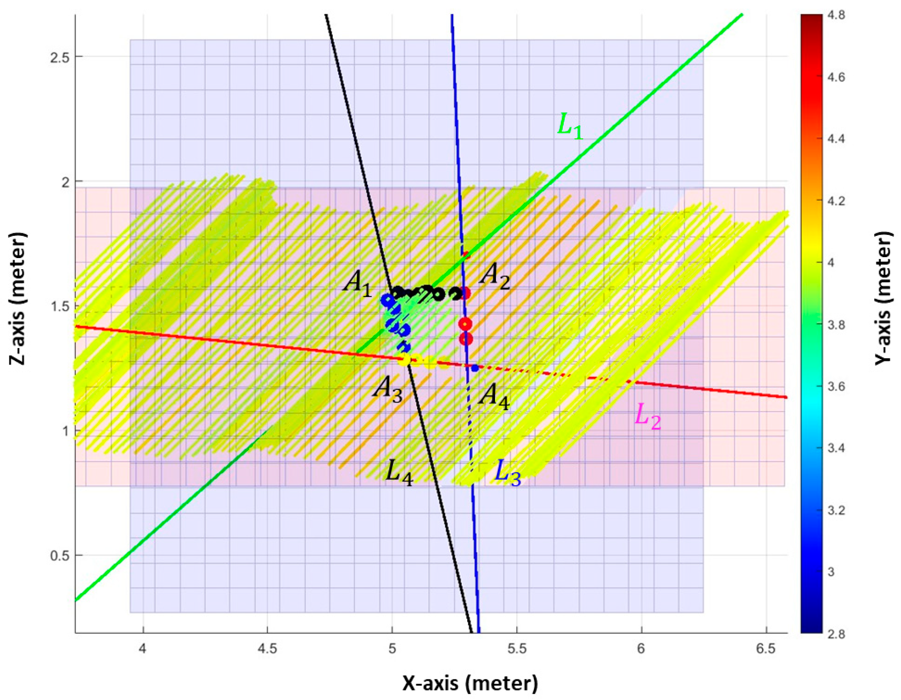
The projected line lies within $\Pi$ under the geometric construction defined above. Intersections of projected lines (e.g., $L_1$ with $L_4$, $L_2$ with $L_3$) are used to estimate corner points $A_1$ through $A_4$ of the rectangular protrusion, as shown in Figure 17.

Geometric dimensions are then estimated as follows:

• Length: average horizontal (X-axis) distances between $A_1-A_2$ and $A_3-A_4$.
• Width: average vertical (Z-axis) distances between $A_1-A_3$ and $A_2-A_4$. All measurements are computed within the common projected plane to maintain geometric consistency under the planar modeling assumptions.
• Height: substitute each corner’s X and Z coordinates into the top and wall plane equations, compute the corresponding Y-values, and average the vertical differences.

(4)

Estimation for circular protrusions

To estimate the radius of a circular protrusion, the 3D boundary points are projected onto the top surface plane (light blue), producing a 2D point set $(x_i,z_i)$. A circle is estimated by minimizing the cost function shown in Equation (24):

$$E=\sum _{i=1}^N{(\sqrt{{(x_i-x_c)}^2+{(z_i-z_c)}^2}-r)}^2$$

(24)

where $(x_c,z_c)$ is the estimated center and $r$ is the radius. The protrusion height is estimated by computing the average Y-value difference between the fitted top surface (light blue) and the adjacent wall surface (light red) along the fitted circle.

All estimations are performed under simulated sensor noise and pose conditions; therefore, reported geometric deviations reflect performance within the HIL simulation framework under the assumptions defined in Section 3 and Section 4 and do not constitute field-validated underwater accuracy.

4.2.3. Mapping Accuracy Under Ideal-Motion and Dynamic-Control Navigation

This section compares the mapping behavior of the laser imaging system under two navigation modes: (a) ideal-motion scanning and (b) dynamic-control scanning within the simulation framework defined in Section 4.1. In both cases, the AUV scans a wall featuring three known protrusions using the same sensors and mapping algorithms.

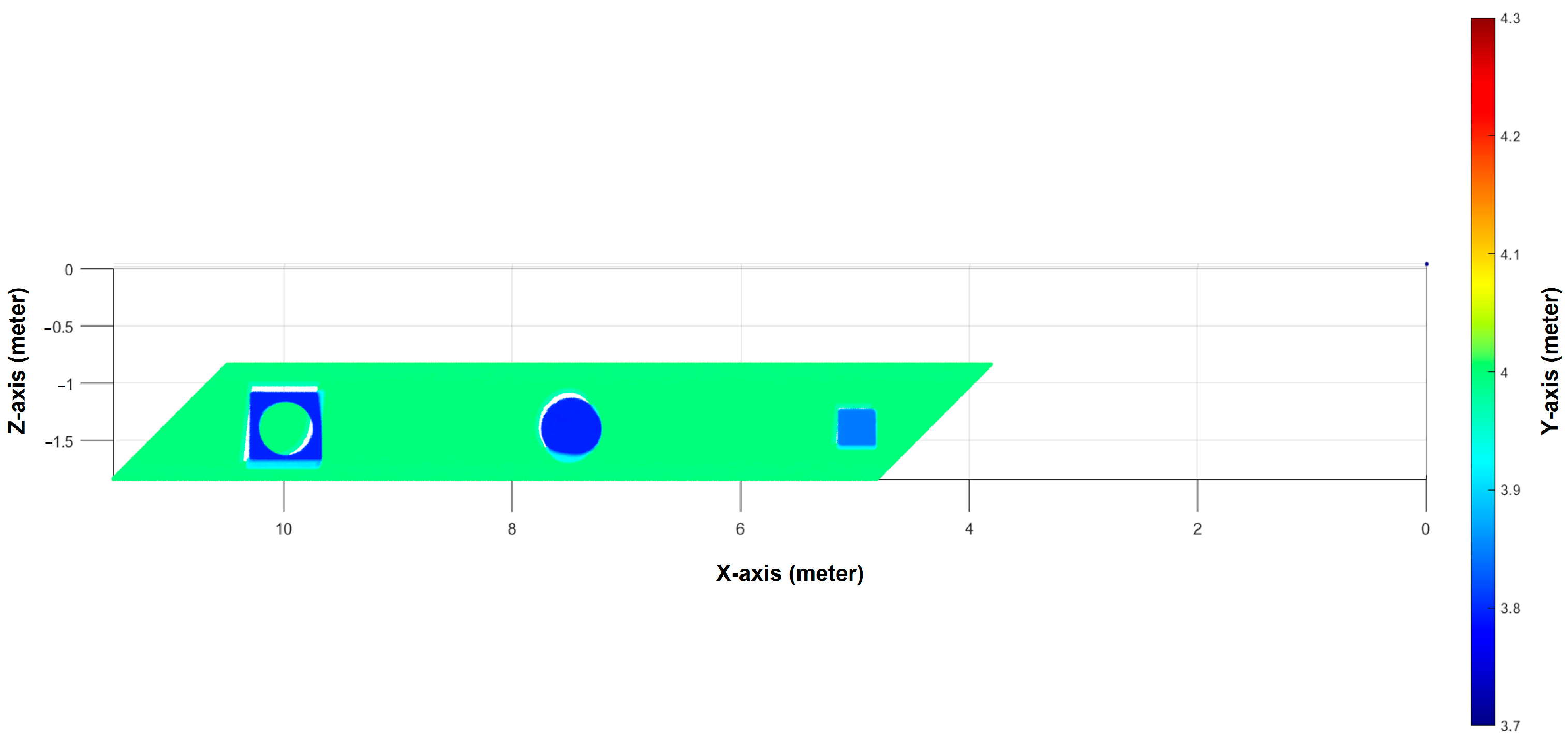
In the ideal-motion scanning mode, the AUV moves at a constant speed and depth while maintaining ideal alignment with the wall—without any heading or position corrections. This produces a smooth trajectory without control-induced disturbances in the simulation model. As shown in Figure 18, observed mapping deviations are primarily associated with geometric and sensing factors within the simulation, including occlusions, laser–camera misalignment, and simulated surface noise.

In the dynamic-control scanning mode, the AUV’s wall-following controller actively adjusts heading and lateral position in response to sensor feedback. This enables adaptive wall tracking but also introduces yaw oscillations and lateral shifts within the control loop, which may distort mapped elevation profiles and generate overlapping or noisy scan regions under the simulated conditions. To quantify relative geometric deviation within the simulation, the relative error is computed using Equation (25):

$$\delta ={\displaystyle \frac{I-M}{I}}\times 100\%$$

(25)

where $\delta$ is the relative error, $I$ is the true geometric value, and $M$ is the estimated value.

(1)

Protrusion 1: Rectangular prism

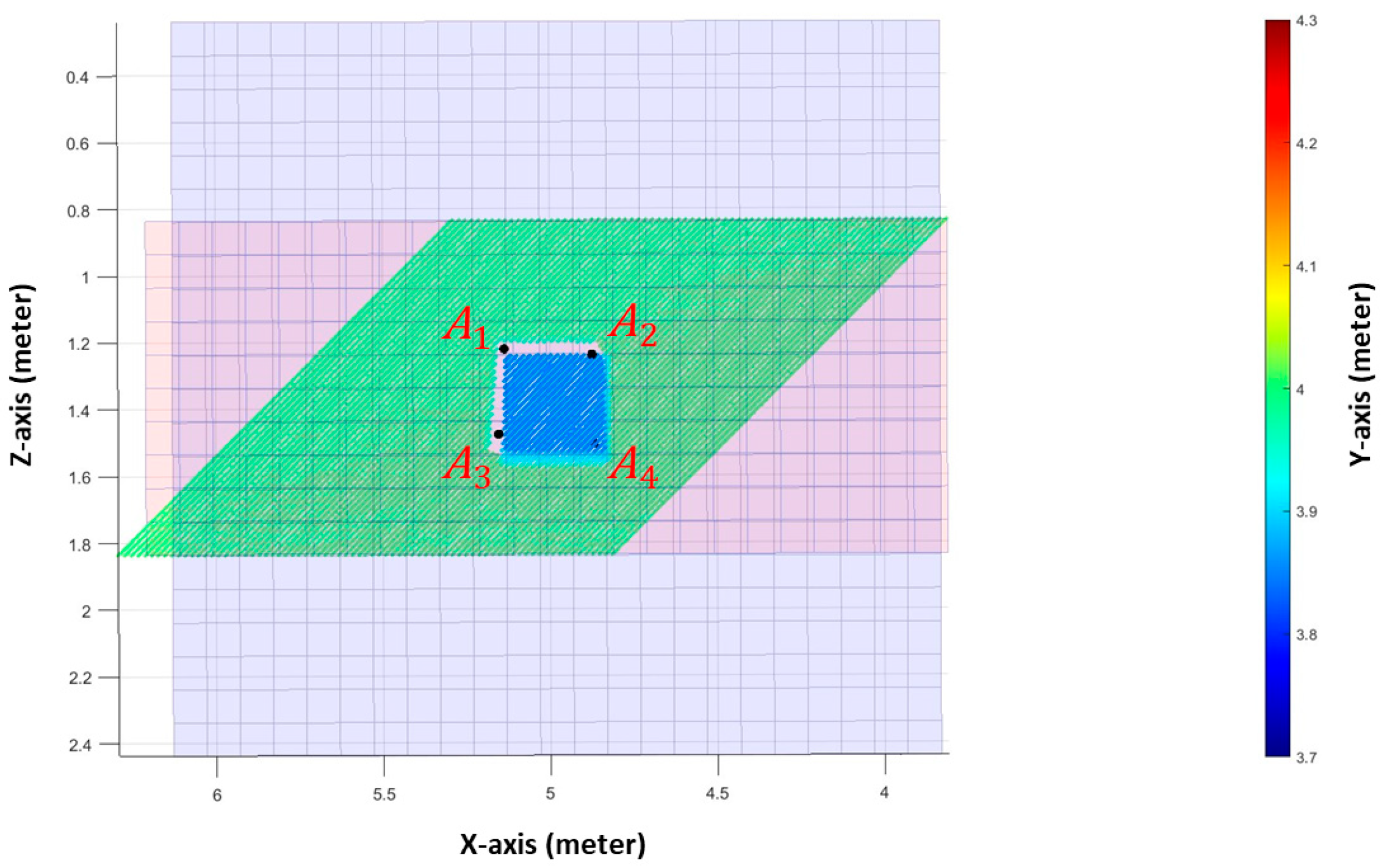
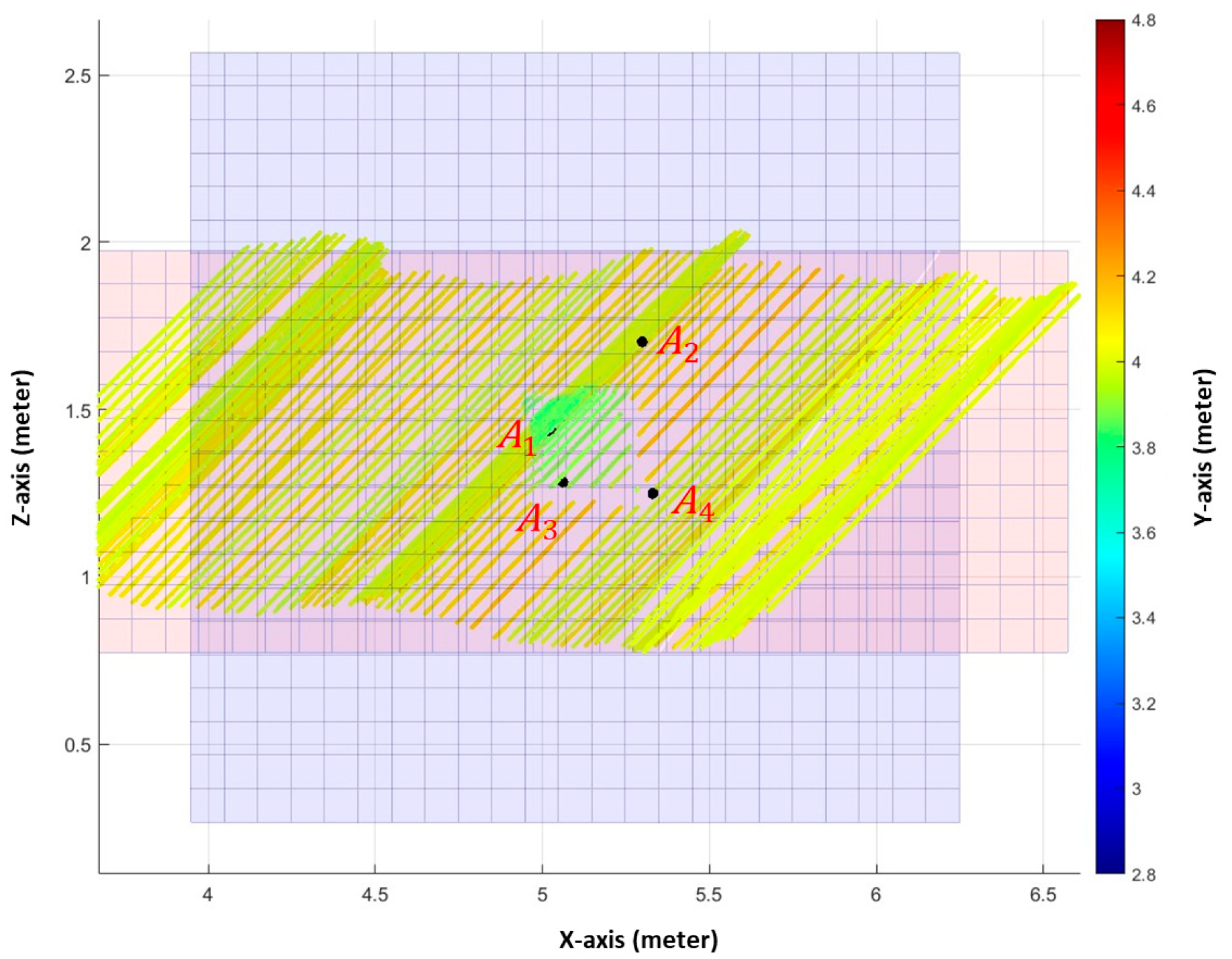
Figure 19 and Figure 20 show the reconstructed elevation maps under ideal-motion and dynamic-control modes, respectively. Both retain the general shape characteristics, while dynamic-control exhibits visible distortions associated with yaw variations.

Table 4. Estimated dimensions of Protrusion 1 (rectangular prism).

	Length (m)	Width (m)	Area (m2)	Height (m)
True value	0.3	0.3	0.09	0.15
Dynamic-control	0.271 (10%)	0.302 (1%)	0.082 (9%)	0.11 (27%)
Ideal-motion	0.317 (5%)	0.264 (13%)	0.084 (6%)	0.146 (3%)

summarizes the estimated dimensions and relative errors. Under dynamic-control, the computed height and area deviations (27% and 9%) are larger than those under ideal-motion (3% and 6%) in this simulation case, with a slightly higher length deviation but a lower width deviation under dynamic-control.

(2)

Protrusion 2: Cylinder

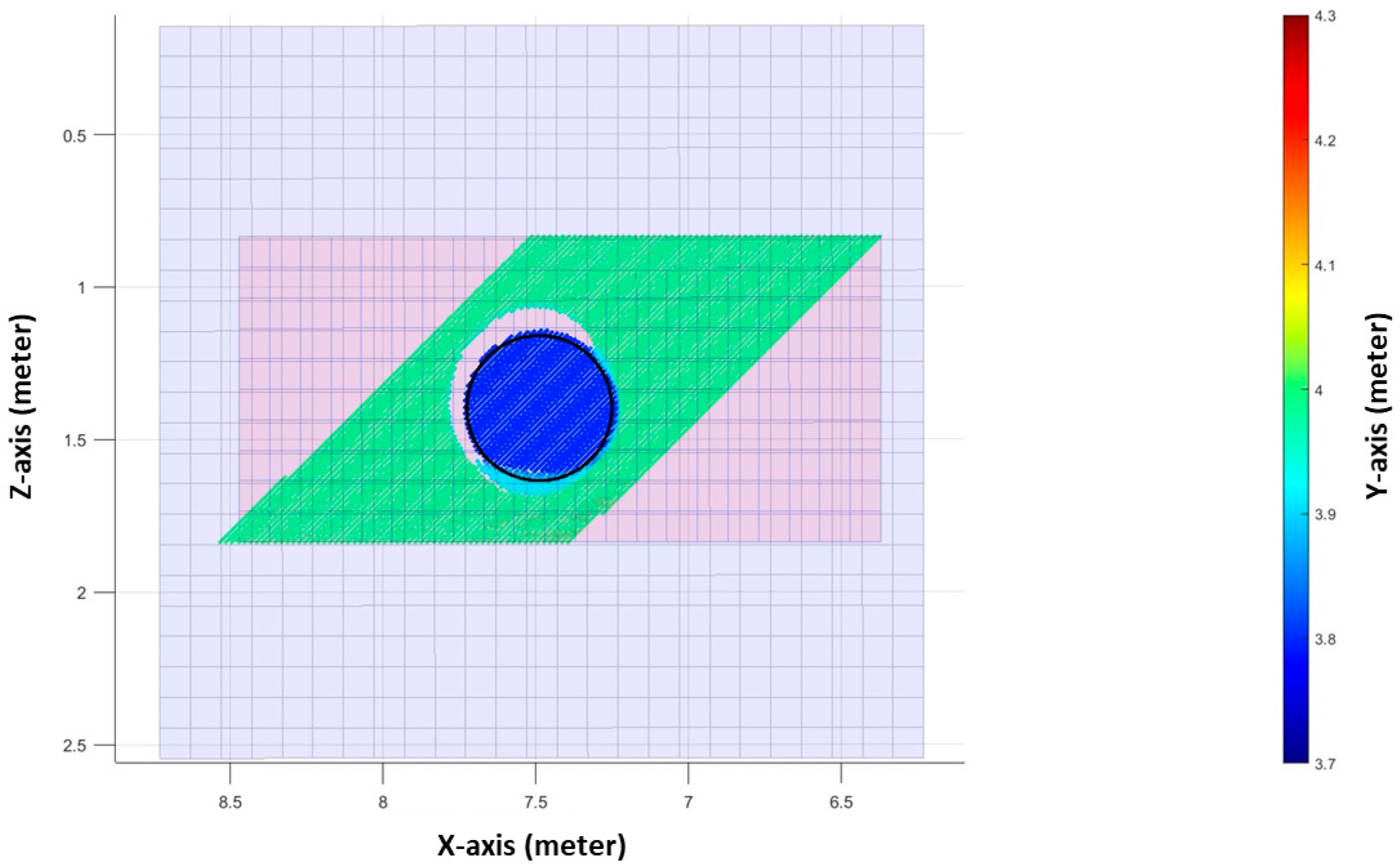
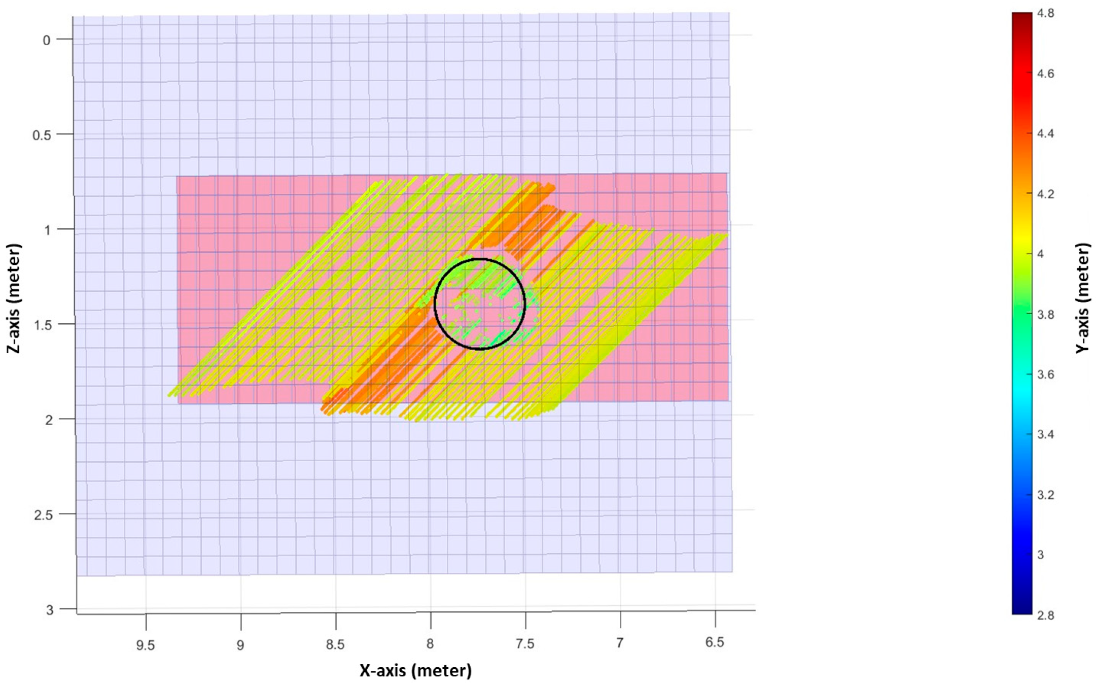
Figure 21 and Figure 22 illustrate mapping results for the cylindrical target. The ideal-motion scan exhibits partial occlusion at the rear edge, while the dynamic-control mode produces redundant scanning that distorts the circular shape.

As shown in

Table 5. Estimated dimensions of Protrusion 2 (cylinder).

	Diameter (m)	Height (m)
True value	0.5	0.2
Dynamic-control	0.475 (5%)	0.16 (20%)
Ideal-motion	0.522 (4%)	0.196 (2%)

, ideal-motion scanning yields smaller diameter and height deviations (4% and 2%) compared to dynamic-control scanning (5% and 20%) in this simulated scenario.

(3)

Protrusion 3: Square frame with internal circular hole

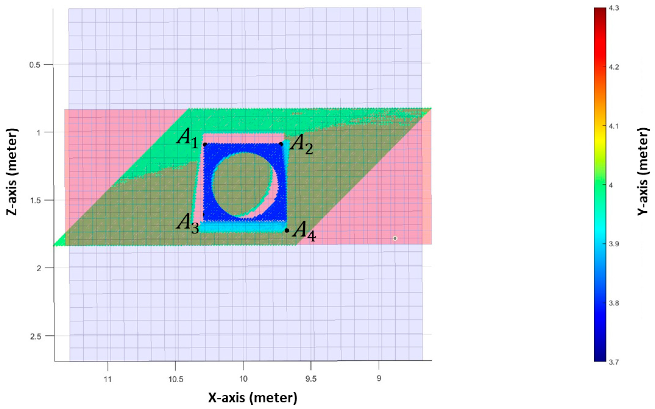
Under ideal-motion (Figure 23), the square frame and internal circle are reconstructed with minor occlusion near the hole. In dynamic-control (Figure 24), yaw oscillations are associated with angular distortions, especially near corners $A_2$ and $A_4$, and increase transformation deviations between image and world coordinates under the geometric mapping model.

Table 6. Estimated dimensions of Protrusion 3 (outer square frame).

	Length (m)	Width (m)	Area (m2)	Height (m)
True value	0.6	0.6	0.36	0.2
Dynamic-control	0.44 (26%)	0.53 (12%)	0.233 (35%)	0.15 (25%)
Ideal-motion	0.581 (3%)	0.574 (4%)	0.36 (8%)	0.186 (7%)

shows that dimension deviations for the square frame are larger in dynamic-control (up to 35% in area and 26% in length), while ideal-motion yields deviations under 8% in this case. For the internal hole,

Table 7. Estimated dimensions of Protrusion 3 (internal circular hole).

	Diam (m)	Height (m)
True value	0.5	0.2
Dynamic-control	0.382 (24%)	0.16 (20%)
Ideal-motion	0.498 (1%)	0.187 (7%)

shows diameter and height deviations of 24% and 20% under dynamic-control, and 1% and 7% under ideal-motion in the simulated configuration.

These results illustrate differences between ideal-motion and dynamic-control scanning strategies within the structured tank simulation. The ideal-motion trajectory provides a disturbance-free reference condition for examining mapping behavior under the assumed sensing and geometric model. In contrast, dynamic-control navigation represents closed-loop control behavior within the simulation, where feedback-based heading corrections introduce yaw fluctuations, variable camera orientations, and surface occlusion. While the control algorithm enables adaptive tracking, it also introduces geometric variability in the reconstructed data, resulting in larger dimensional deviations across the three protrusions in this simulated tank scenario.

4.3. Frontal Wall Collision Avoidance Performance

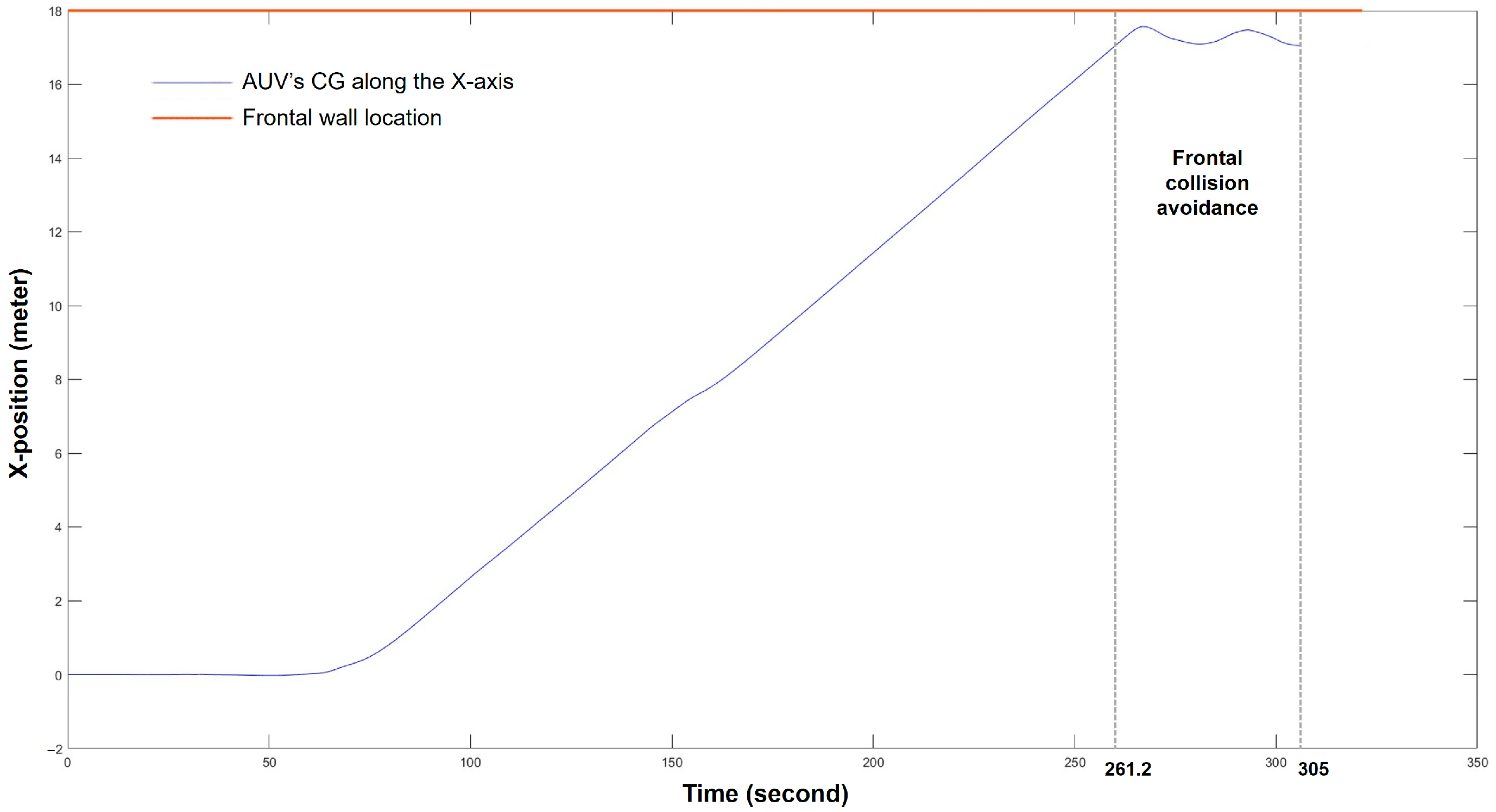
In the final phase of the wall-following simulation, the AUV was tasked with avoiding a frontal wall perpendicular to the inspection wall. The maneuver began at t = 261.2 s and ended at t = 305 s, spanning 43.8 s. Building upon the setup described in Section 4.1, this scenario examines the AUV’s response to detecting and avoiding an approaching frontal wall while attempting to maintain alignment with the original inspection surface in the simulation framework.

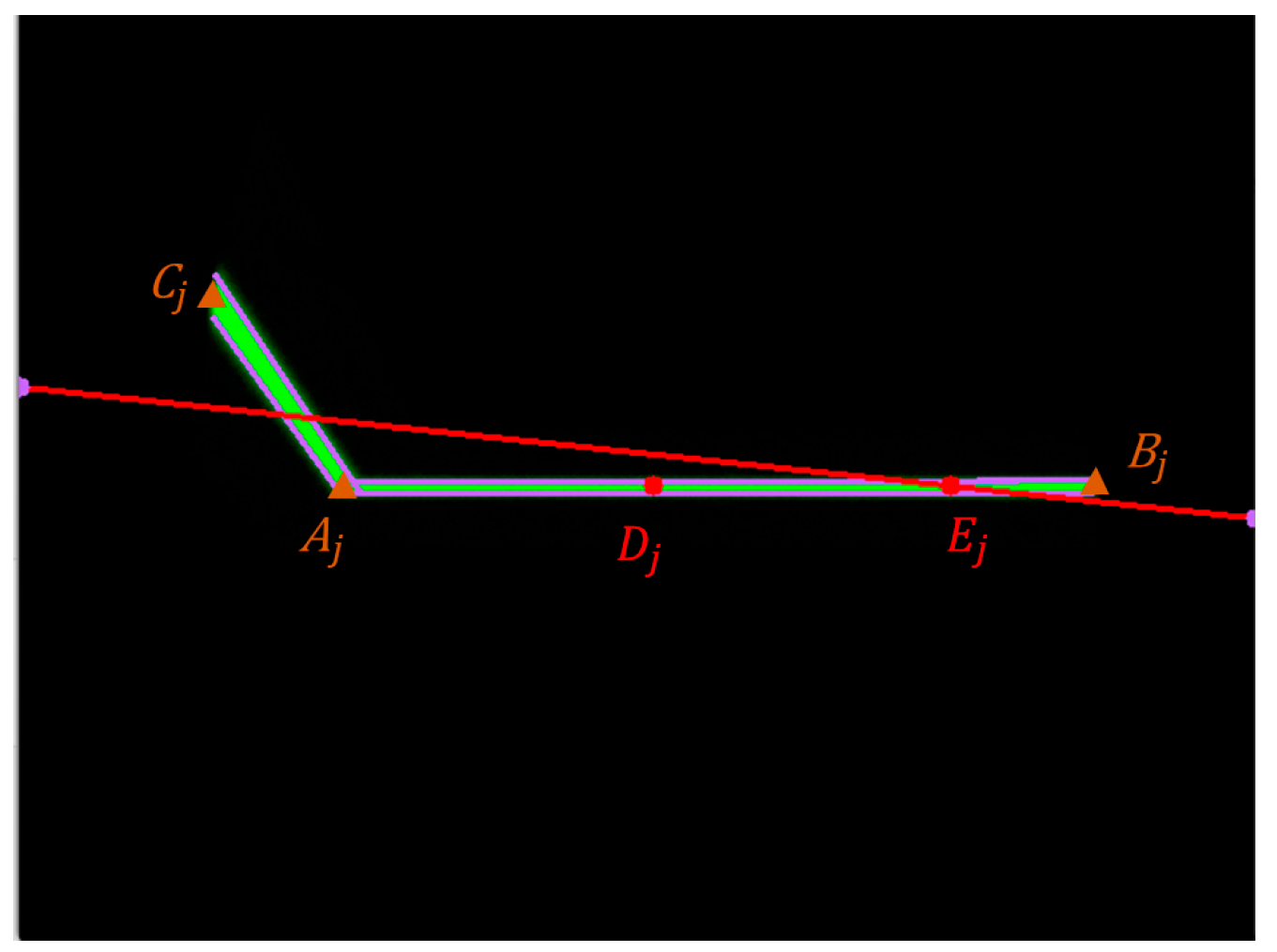
The AUV employed the same single-line laser imaging system used for side-wall-following, but with a different image processing strategy. As shown in Figure 25, applying the PHT used for laser line orientation estimation may produce unreliable results when a frontal wall is present under the assumed geometric conditions. Vertical laser line segments (e.g., $\overline{C_j{A}_j}$) may be misclassified as side-wall features, which can result in inaccurate yaw angle estimates and ineffective corrective commands within the control loop.

This behavior can cause the AUV to rotate in place rather than initiating a proper avoidance maneuver under the simulated conditions. To address this, the system bypasses the PHT-based orientation method and instead uses brightness centroid analysis. For each image, intensity centroids (e.g., $D_j$ and $E_j$) are extracted along selected columns and used to estimate the yaw angle ${\psi }_A$ and the distance to the frontal wall within the geometric estimation framework. This method provides more stable yaw and distance estimates when the laser stripe spans perpendicular surfaces in the simulated tank environment.

Figure 26 plots the AUV’s Earth-fixed X-axis position. The frontal wall is located at X = 18 m. After detecting the wall at t = 261.2 s, the AUV decelerated and came to a stop by t = 305 s. The minimum clearance during this process was 1.04 m, indicating non-contact avoidance in the simulated scenario. The mean yaw deviation relative to the simulated ground truth was 1.76° (standard deviation: 4.73°), while the mean distance deviations to the right and frontal walls were 0.01 m and 0.03 m (standard deviations: 0.04 m for both) over the analyzed interval under the simulation conditions.

4.4. Discussion and Limitations

The results presented in Section 4.2 and Section 4.3 indicate that a single-line laser imaging system can support closed-loop wall-following, geometric mapping, and frontal collision avoidance within a structured and confined inspection scenario under hardware-in-the-loop simulation conditions.

The evaluation highlights several key system-level observations. First, the comparison between ideal-motion and dynamic-control navigation modes illustrates the influence of vehicle attitude dynamics on mapping deviations within the simulation. Under ideal-motion scanning, observed mapping deviations are primarily associated with geometric projection effects, stripe extraction variability, and local occlusion. In contrast, dynamic-control scanning introduces yaw oscillations and lateral deviations caused by feedback-based heading corrections within the control loop. These motion-induced variations propagate through the image-to-world transformation and are associated with larger dimensional deviations across the protrusion types. The results therefore distinguish perception-related deviations from control-related geometric distortions within the simulation, providing insight into the sensitivity of laser-based mapping to vehicle motion stability.

Second, the frontal wall avoidance experiment demonstrates that orientation estimation strategies must adapt to geometric context within the defined simulation conditions. The probabilistic Hough transform (PHT), effective during side-wall-following, may produce unreliable orientation estimates when perpendicular surfaces generate vertical stripe segments. Replacing PHT with brightness-centroid-based estimation during frontal approach provides more stable orientation estimates in this specific geometric configuration. This illustrates that perception modules in laser-guided inspection systems may require context-aware switching rather than a single universal estimator.

Despite these observations, several limitations must be clearly acknowledged:

(1)

Simulation-Based Evaluation

All results are obtained within a hardware-in-the-loop simulation framework. Although the onboard controller, communication architecture, update rates, and control signals are preserved, environmental disturbances such as currents, turbulence, wall-induced hydrodynamic interactions, and sensor latency variability are not modeled. Therefore, reported performance reflects algorithmic and geometric behavior within a controlled simulation environment and should be interpreted as a feasibility-level evaluation rather than validated underwater field performance.

(2)

Optical Simplifications

The laser imaging model assumes idealized optical propagation without turbidity, scattering, absorption variability, or specular reflection effects. Real underwater environments may degrade stripe visibility, distort intensity distribution, or introduce false features. The adopted brightness threshold and centroid parameters are tuned for the simulated environment and may require reconfiguration under real optical conditions.

(3)

Structured Geometric Assumption

The mode-switching logic and frontal detection thresholds assume orthogonal wall intersections within a rectangular tank geometry. The angular criteria used for switching between wall-following and avoidance are not intended as general solutions for arbitrary architectural layouts or curved structures. Extension to irregular or non-orthogonal environments would likely require adaptive geometric modeling.

(4)

Single-Sensor Configuration

The framework deliberately employs a single-line laser and monocular camera to evaluate a low-complexity configuration. While this simplifies system integration and reduces hardware requirements, it provides less redundancy than multi-sensor fusion architectures incorporating sonar, stereo vision, or inertial–visual coupling. This design therefore represents a trade-off between system simplicity and cost on one hand, and sensing robustness and redundancy on the other, and the present study focuses on establishing a baseline reference for such a low-complexity configuration.

(5)

Control–Perception Coupling Sensitivity

The dynamic-control results indicate that mapping deviations increase with yaw oscillations and lateral correction magnitude within the simulation. This suggests that high-resolution geometric reconstruction using single-line laser sensing is sensitive to trajectory stability under the modeled conditions. Future implementations may require improved heading damping or trajectory smoothing to mitigate control-induced mapping distortion.

Overall, the presented framework is positioned as a system-level feasibility study for near-field, structured inspection using a compact single-line laser configuration. The results demonstrate geometric coherence and closed-loop integration under controlled simulation assumptions, while delineating the gap between simulation-based evaluation and operational deployment.

Future work will include controlled water-tank experiments to assess optical robustness and to evaluate the performance of the proposed perception and mapping algorithms under realistic optical disturbances such as turbidity and scattering, incorporation of simplified hydrodynamic disturbance models into the HIL framework, and refinement of motion stabilization strategies to reduce control-induced mapping distortion.

5. Conclusions

This study presented and examined a single-line laser-based wall-following and mapping framework for autonomous underwater vehicles operating in structured, confined environments under simulation conditions. The main findings are summarized as follows:

• Integrated perception–control framework:
  A unified geometric formulation was developed to estimate yaw deviation, lateral wall distance, and frontal distance from a single projected laser stripe. The same image stream is used for both real-time wall-following control and post-mission geometric reconstruction within the simulation framework.
• Controlled evaluation using HIL simulation:
  A hardware-in-the-loop platform was constructed to emulate onboard computation, sensor feedback, and closed-loop actuation. This configuration allowed geometric sensing behavior to be examined independently of environmental and hydrodynamic disturbances within the simulation model.
• Wall-following stability:
  Under closed-loop navigation within the simulation, the AUV maintained the prescribed wall offset with small steady-state deviations, indicating that a single-line laser can provide geometric feedback suitable for parallel tracking in structured settings.
• Mapping accuracy under different navigation modes:
  Ideal-motion scanning provided a baseline reference condition for geometric reconstruction, with comparatively small dimensional deviations. In contrast, dynamic-control navigation introduced yaw oscillations and lateral misalignment, which were associated with larger reconstruction deviations while preserving overall feature recognizability in the simulated results. This comparison illustrates the influence of control-induced motion disturbances on laser-based mapping deviations within the simulation.
• Frontal obstacle avoidance behavior
  When a perpendicular wall was introduced, a centroid-based estimation strategy provided more stable orientation estimates compared to line-based orientation estimation in this configuration. The vehicle executed a deceleration maneuver while maintaining non-contact clearance within the simulation, illustrating adaptive mode switching within the same sensing architecture.
• Scope and limitations:
  The evaluation was conducted in a structured rectangular tank environment under simulated optical conditions. Hydrodynamic disturbances, water turbidity, refraction effects, and actuator nonlinearities were not explicitly modeled. Therefore, the reported results represent a controlled performance reference rather than a full-field deployment validation.

The presented framework focuses on a compact single-sensor configuration to evaluate feasibility under controlled conditions, and future extensions may consider integration with complementary sensing modalities to enhance robustness in more complex environments. Overall, the results indicate that a compact single-line laser configuration is capable of supporting integrated wall-following and surface mapping within structured inspection scenarios under simulated conditions. Future work will focus on experimental validation in water tank trials, including evaluation of robustness under optical disturbances such as turbidity and scattering, and on incorporating environmental disturbances and sensor uncertainties into the perception–control framework.

References

1. ICOLD-CIGB. World Register of Dams: General Synthesis. Available online: https://www.icold-cigb.org/GB/world_register/general_synthesis.asp (accessed on 17 March 2026).
2. Kondo, H.; Ura, T. Navigation of an AUV for investigation of underwater structures. Control Eng. Pract. 2004, 12, 1551–1559. [Google Scholar] [CrossRef]
3. Kondo, H.; Maki, T.; Ura, T.; Nose, Y.; Sakamaki, T.; Inaishi, M. Relative navigation of an autonomous underwater vehicle using a light-section profiling system. In Proceedings of the 2004 IEEE/RSJ International Conference on Intelligent Robots and Systems (IROS) (IEEE Cat. No.04CH37566); IEEE: New York, NY, USA, 2004; pp. 1103–1108. [Google Scholar]
4. Kondo, H.; Maki, T.; Ura, T.; Nose, Y.; Sakamaki, T.; Inaishi, M. Structure tracing with a ranging system using a sheet laser beam. In Proceedings of the 2004 International Symposium on Underwater Technology (IEEE Cat. No.04EX869); IEEE: New York, NY, USA, 2004; pp. 83–88. [Google Scholar]
5. Maki, T.; Mizushima, H.; Ura, T.; Sakamaki, T.; Yanagisawa, M. AUV navigation around jacket structures I: Relative localization based on multi-sensor fusion. J. Mar. Sci. Technol. 2012, 17, 330–339. [Google Scholar] [CrossRef]
6. Maki, T.; Ura, T.; Sakamaki, T. AUV navigation around jacket structures II: Map based path-planning and guidance. J. Mar. Sci. Technol. 2012, 17, 523–531. [Google Scholar] [CrossRef]
7. Albiez, J.; Duda, A.; Fritsche, M.; Rehrmann, F.; Kirchner, F. CSurvey—An autonomous optical inspection head for AUVs. Robot. Auton. Syst. 2015, 67, 72–79. [Google Scholar] [CrossRef]
8. Jacobi, M. Autonomous inspection of underwater structures. Robot. Auton. Syst. 2015, 67, 80–86. [Google Scholar] [CrossRef]
9. Inzartsev, A.; Eliseenko, G.; Panin, M.; Pavin, A.; Bobkov, V.; Morozov, M. Underwater pipeline inspection method for AUV based on laser line recognition: Simulation results. In Proceedings of the 2019 IEEE Underwater Technology (UT); IEEE: New York, NY, USA, 2019; pp. 1–8. [Google Scholar]
10. Bodenmann, A.; Thornton, B.; Ura, T. Development of long range color imaging for wide area 3D reconstructions of the seafloor. In Proceedings of the 2013 IEEE International Underwater Technology Symposium (UT); IEEE: New York, NY, USA, 2013; pp. 1–5. [Google Scholar]
11. Nakatani, T.; Li, S.; Ura, T.; Bodenmann, A.; Sakamaki, T. 3D visual modeling of hydrothermal chimneys using a rotary laser scanning system. In Proceedings of the 2011 IEEE Symposium on Underwater Technology and Workshop on Scientific Use of Submarine Cables and Related Technologies; IEEE: New York, NY, USA, 2011; pp. 1–5. [Google Scholar]
12. Prats, M.; Fernández, J.J.; Sanz, P.J. Combining template tracking and laser peak detection for 3D reconstruction and grasping in underwater environments. In Proceedings of the 2012 IEEE/RSJ International Conference on Intelligent Robots and Systems; IEEE: New York, NY, USA, 2012; pp. 106–112. [Google Scholar]
13. Caccia, M. Laser-triangulation optical-correlation sensor for ROV slow motion estimation. IEEE J. Ocean. Eng. 2006, 31, 711–727. [Google Scholar] [CrossRef]
14. Hu, Q.; Zhu, H.; Yu, M.; Fan, Z.; Zhang, W.; Liu, X.; Li, Z. A novel 3D detection system with target keypoint estimation for underwater pipelines. Ocean. Eng. 2024, 309, 118319. [Google Scholar] [CrossRef]
15. Chou, Y.-C.; Huang, J.-H. Preliminary evaluation of an AUV equipped with a line laser for wall following and mapping in a rectangular tank. In Proceedings of the OCEANS 2024-Halifax; IEEE: New York, NY, USA, 2024; pp. 1–5. [Google Scholar]
16. Fossen, T.I. Guidance and Control of Ocean Vehicles; Wiley: Hoboken, NJ, USA, 1994. [Google Scholar]
17. Wang, C.-C.; Cheng, M.-S. Nonmetric camera calibration for underwater laser scanning system. IEEE J. Ocean. Eng. 2007, 32, 383–399. [Google Scholar] [CrossRef]
18. Kiryati, N.; Eldar, Y.; Bruckstein, A.M. A probabilistic Hough transform. Pattern Recognit. 1991, 24, 303–316. [Google Scholar] [CrossRef]
19. Chou, Y.-C.; Chen, H.-H.; Wang, C.-C.; Wang, C.-C.; Chen, W.-H. A hardware-in-the-loop simulation platform for development of auv control systems. In Proceedings of the 2019 IEEE Underwater Technology (UT); IEEE: New York, NY, USA, 2019; pp. 1–6. [Google Scholar]
Figure 1. Geometric layout of the single-line laser imaging system and thruster configuration on the IUT AUV-I.
Jmse 14 00680 g001
Figure 2. Relative geometry of the AUV, laser imaging system, and wall surface.
Jmse 14 00680 g002
Figure 3. Geometric interpretation of distance and angular parameters on the laser plane.
Jmse 14 00680 g003
Figure 4. Illustration of yaw-induced misalignment between the laser stripe and wall surface, where a denotes the position vector of the laser in the body-fixed frame.
Jmse 14 00680 g004
Figure 5. Determination of perpendicular distance from the AUV’s CG to the wall, where P w a l l and P y denotes points along the projected line used to determine the perpendicular distance d C G .
Jmse 14 00680 g005
Figure 6. Geometric parameters used for wall-following control under planar wall assumptions, including front and rear distances to the wall ( d f , d b ), where ( x w a l l , y w a l l ) denote the coordinates of P w a l l in the Earth-fixed frame.
Jmse 14 00680 g006
Figure 7. Geometric interpretation of frontal distance d C G f relative to the AUV CG and projected laser point under planar wall assumptions.
Jmse 14 00680 g007
Figure 8. AUV wall-following and scanning strategy within the structured rectangular tank simulation. The arrows indicate the desired moving directions of the AUV.
Jmse 14 00680 g008
Figure 9. Schematic of frontal wall detection from laser stripe geometry under planar and orthogonal wall assumptions.
Jmse 14 00680 g009
Figure 11. Geometric configurations of three wall-mounted protrusions used to evaluate wall-following behavior and mapping performance within the structured simulation environment.
Jmse 14 00680 g011
Figure 12. Yaw angle ψ A and perpendicular distance d C G compared to simulation ground truth and target values during wall-following in the structured protrusion simulation.
Jmse 14 00680 g012
Figure 13. Distance errors in front-right d f and rear-right d b distances relative to the 1.5 m target during wall-following in the protrusion simulation scenario.
Jmse 14 00680 g013
Figure 14. Simulated mapped wall elevation with protrusions, derived from fused sensor outputs within the HIL framework.
Jmse 14 00680 g014
Figure 15. Edge point selection: (left)—original laser image; (right)—processed image after brightness centroid-based extraction with edge points M P and N P marked.
Jmse 14 00680 g015
Figure 16. Region-based classification of boundary points for rectangular feature estimation, showing regions A 1 A 4 used for dimension estimation under planar surface assumptions.
Jmse 14 00680 g016
Figure 17. Fitted line segments ( L 1 L 4 ) and intersection points ( A 1 A 4 ) projected onto the top surface plane for rectangular protrusion dimension estimation within the geometric modeling framework, showing the fitted top surface (light blue) and surrounding wall plane (light red).
Jmse 14 00680 g017
Figure 18. Mapped wall elevation profile under ideal-motion scanning, showing three geometric protrusions.
Jmse 14 00680 g018
Figure 19. Reconstructed mapping of Protrusion 1 under ideal-motion scanning, showing the mapped wall elevation profile (other colors), fitted top surface (light blue), surrounding wall plane (light red), and corner points A 1 A 4 .
Jmse 14 00680 g019
Figure 20. Reconstructed mapping of Protrusion 1 under dynamic-control scanning, showing the mapped wall elevation profile (other colors), fitted top surface (light blue), surrounding wall plane (light red), and corner points A 1 A 4 .
Jmse 14 00680 g020
Figure 21. Reconstructed mapping of Protrusion 2 under ideal-motion scanning, showing the mapped wall elevation profile (other colors), fitted top surface (light blue), surrounding wall plane (light red), and the estimated circular boundary.
Jmse 14 00680 g021
Figure 22. Reconstructed mapping of Protrusion 2 under dynamic-control scanning, showing the mapped wall elevation profile (other colors), fitted top surface (light blue), surrounding wall plane (light red), and the estimated circular boundary.
Jmse 14 00680 g022
Figure 23. Reconstructed mapping of Protrusion 3 under ideal-motion scanning, showing the mapped wall elevation profile (other colors), fitted top surface (light blue), surrounding wall plane (light red), corner points A 1 A 4 of the outer square frame, and the estimated circular boundary of the inner hole.
Jmse 14 00680 g023
Figure 24. Reconstructed mapping of Protrusion 3 under dynamic-control scanning, showing the mapped wall elevation profile (other colors), fitted top surface (light blue), surrounding wall plane (light red), corner points A 1 A 4 of the outer square frame, and the estimated circular boundary of the inner hole.
Jmse 14 00680 g024
Figure 25. Example of inaccurate yaw angle estimation by the PHT during simulated frontal wall approach, where incorrect line detection arises from misclassification of vertical stripe segments at wall intersections as side-wall features.
Jmse 14 00680 g025
Figure 26. Time-series of the AUV’s Earth-fixed X-position during simulated frontal wall avoidance, with the front wall located at X = 18 m and the avoidance interval indicated.
Jmse 14 00680 g026