Article

Unsteady Cavitation Flow Characteristics Around the Clark-Y Hydrofoil Cascade

1
Harbin Institute of Technology, Harbin 150001, China
2
Beijing Institute of Astronautical Systems Engineering, Beijing 100076, China
3
School of Mechanical Engineering, Beijing Institute of Technology, Beijing 100811, China
*
Author to whom correspondence should be addressed.
J. Mar. Sci. Eng. 2026, 14(7), 620; https://doi.org/10.3390/jmse14070620
Submission received: 9 February 2026 / Revised: 14 March 2026 / Accepted: 16 March 2026 / Published: 27 March 2026
(This article belongs to the Section Ocean Engineering)

Abstract

Both experimental and numerical studies were conducted to obtain the influence laws of complex cavitation flow structures around a Clark-Y hydrofoil cascade. The similarities and differences in cavitation flow characteristics between the cascade and single hydrofoil were compared to analyze the influence of the cascade configuration on the flow field structure. This study focuses on the correlations among cavity development, lift–drag characteristics, and flow field features of the hydrofoil cascade. The results indicate significant differences in the development degree and history of cavities at different positions within the cascade. The top layer of the cascade exhibits a cavitation pattern similar to a single hydrofoil; both generate large-scale shedding vortices at the trailing edge. In contrast, the cavitation phenomena in the middle and bottom layers are similar to each other. The suction side of the top-layer hydrofoil influences the middle and bottom layers. This interaction suppresses the formation of large-scale shedding bubbles and subsequently hinders re-entrant shocks. Furthermore, the cavities in the middle and bottom layers develop more rapidly, causing the dynamic characteristics of the cascade to reach their peak values earlier. At the cloud cavitation stage, the Strouhal numbers ( S t ) for cavity collapse on the top and bottom hydrofoils are approximately 0.2 and 0.3, respectively. The S t for the middle hydrofoil exhibits an intermediate value that decreases from 0.3 to 0.2 as the cavitation number ( σ ) declines, reflecting a transitional characteristic modulated by the cascade structure. Compared to a single hydrofoil, the cascade is subject to the combined effects of the three-layer hydrofoils; consequently, its lift is approximately three times that of a single hydrofoil, though its drag also increases threefold. The lift variation pattern of the top-layer hydrofoil in the cascade is similar to that of a single hydrofoil. In contrast, the middle-layer hydrofoil exhibits a more complex lift evolution, as both its suction and pressure sides are significantly influenced by the surrounding cascade structure. For the bottom-layer hydrofoil, the lift remains relatively low because no cavities are generated on its surface. Lift fluctuation frequencies that aligned with cavity collapse were identified at 45 Hz, 70 Hz, and 50 Hz across the top, middle, and bottom cascade layers, respectively.

1. Introduction

With the rapid advancement of the aerospace industry, reusable rockets have emerged as a significant milestone in space history, following the development of artificial satellites and manned spaceflight [1]. A unique feature of their design is the grid fin, which consists of numerous thin grid walls embedded within a frame [2]. Research indicates that, compared to conventional single-wing configurations, the multi-wing structure of grid fins offers superior aerodynamic characteristics, such as a higher lift-to-area ratio and an exceptional strength-to-weight ratio. Furthermore, grid fins provide significant advantages in terms of compact dimensions and ease of installation [3,4].
Although grid fins have been widely utilized in rocket launches, their application in the field of underwater vehicles remains shrouded in numerous mysteries. There are significant disparities between the hydrodynamic characteristics of underwater grid fins and their aerodynamic counterparts. Furthermore, when underwater vehicles travel at high speeds, cavitation inevitably occurs [5,6], thereby altering the lift and drag characteristics of the grid fins [7]. Investigating the underwater dynamics of grid fins is challenging due to manufacturing difficulties and complex cavitation flow structures [8,9].
Currently, scholars in hydraulic machinery and underwater vehicles are primarily focused on the cavitation phenomena of hydrofoils and cascades [10,11]. They have discovered that hydrofoil structures can effectively mitigate cavitation while demonstrating excellent performance in increasing lift and reducing drag. The representative Clark-Y profile is widely utilized in various apparatuses, including propeller blades, pump-jet impellers, and underwater launching systems. Ji et al. [12] explored the relationship between attached cavities, vortices, and re-entrant jets during the typical evolution of hydrofoil cavitation and numerically simulated the quasi-periodic behavior of attached cavities induced by re-entrant jets. Based on a multi-scale Euler–Lagrange approach, Wang et al. [13] elucidated the significant influence of re-entrant jets on bubble generation and motion around the Clark-Y hydrofoil. Qu et al. [14] employed Large Eddy Simulation (LES) combined with various vortex identification methods to investigate the transient sheet and cloud cavitation flows over a Clark-Y hydrofoil. Their results demonstrated that cavity shedding and collapse are closely correlated with vortex structures. Movahedian et al. [15] integrated LES and Volume of Fluid (VOF) methods to reveal the turbulent characteristics of unsteady cavitating flows around a twisted 3D NACA 16012 hydrofoil, reporting predicted results for pressure, velocity, streamlines, water volume fraction, and turbulent kinetic energy. Su et al. [16] conducted hydrodynamic research on grid fins with different shapes, finding that those with sharp leading edges can significantly enhance the lift-to-drag ratio, thereby improving hydrodynamic performance. Ma et al. [17] investigated the influence of wake interaction on the response of two tandem oscillating hydrofoils; their results indicated that because the downstream hydrofoil is situated in the wake of the upstream one, the upstream hydrofoil exhibits superior heave amplitude and energy extraction performance. Furthermore, increasing the spacing between hydrofoils does not necessarily diminish the disparity between their responses. Raj et al. [18] studied the pitching jet deflection of two side-by-side hydrofoils in a quiescent fluid, demonstrating that the propulsion and maneuverability of unmanned vehicles can be achieved by adjusting key parameters. Yu et al. [19] investigated the cavity development characteristics of a Clark-Y cascade during the cloud cavitation stage from the perspective of vortex dynamics. Similarly, Xu et al. [20] proposed a vortex prediction formula based on force analysis. Zhao et al. [21] studied the effects of hydrofoil profiles and angles of attack on the cavitation number and lift–drag characteristics of the cascade. Based on an aeroelastic analysis method, Ye et al. [22] examined the impact of Mach number variations on the flow field and flutter characteristics of grid fins; their results indicated that at subsonic speeds, the grid fin accelerates the airflow, leading to the premature appearance of transonic flutter ’dip’ characteristics. Furthermore, Zhu et al. [23] developed a negative pressure gradient hydrofoil using non-separation flow theory. They numerically compared its lift, drag, and pressure distribution to the NACA0015 hydrofoil across various cavitation numbers and angles of attack. Additionally, Bublík et al. [24] employed a convolutional neural network to develop a computational model for simulating unsteady flow fields in vibrating cascades, significantly reducing the computational overhead. To date, research by other scholars has mainly concentrated on cavitation characteristics around single hydrofoils or double-layer cascades, with little attention paid to the cavitation phenomena at different positions within multi-layer cascades. Therefore, this paper analyzes the differences in cavitation flow across various layers of a cascade and explores the fundamental causes of these disparities.
Based on experimental observations and numerical simulations of grid fins, this study investigates flow control technology for grid fins during underwater vertical launching. Flow field measurements of the grid fins under fully wetted conditions were conducted to analyze the influence mechanisms of grid fins on the unsteady development of cavitation. Furthermore, this research aims to elucidate the evolution of cavitation behavior and hydrodynamic characteristics of the cascade from the perspective of flow feature analysis, thereby clarifying the regulatory effects of the grid fins.

2. Materials and Methods

2.1. Experimental Methods

2.1.1. Cavitation Water Tunnel

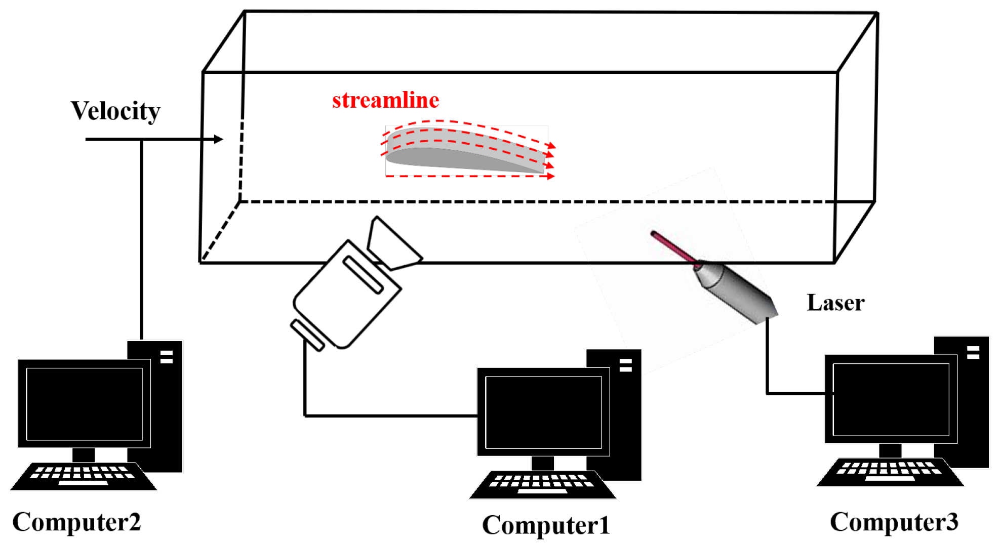
The experiments in this study were conducted in a closed-loop cavitation water tunnel, as shown in Figure 1. The circulation within the tunnel is driven by a 55 kW motor, with the motor speed controlled in real time through a variable frequency drive (VFD) to regulate the flow velocity in the test section. The VFD operates within a range of 0–55 Hz with a control precision of 0.01 Hz, enabling a flow velocity range of 0–20 m/s, though the velocities used in this experiment primarily ranged from 2 to 12 m/s. The flow field pressure was regulated with a vacuum pump to maintain the model at various cavitation numbers. Specifically, the vacuum pump operated from 0 to 90 kPa with a control precision of 0.005 MPa and was equipped with a precision control system to ensure the flow field remained stable at the set pressure value. Based on the Kline–McClintock method, the calculated uncertainty of the cavitation number σ under the experimental conditions was approximately ± 0.01 . To ensure the stability of cavitation nuclei, identical water quality was used for each experiment. A water storage tank was located beneath the tunnel, and a submersible pump was used to fill the entire pipeline before each test. A large tank was situated upstream of the water tunnel, containing guide vanes that effectively separate bubbles and reduce turbulence intensity to minimize interference with the test section. Additionally, the water tunnel was equipped with flow meters, thermometers, and pressure gauges for the real-time monitoring and storage of flow field data. High-speed camera images were captured at a resolution of 1024 × 1024 pixels, with a frame rate of 50,000 fps and an exposure time of 1/50,000 s.

2.1.2. Experimental Model

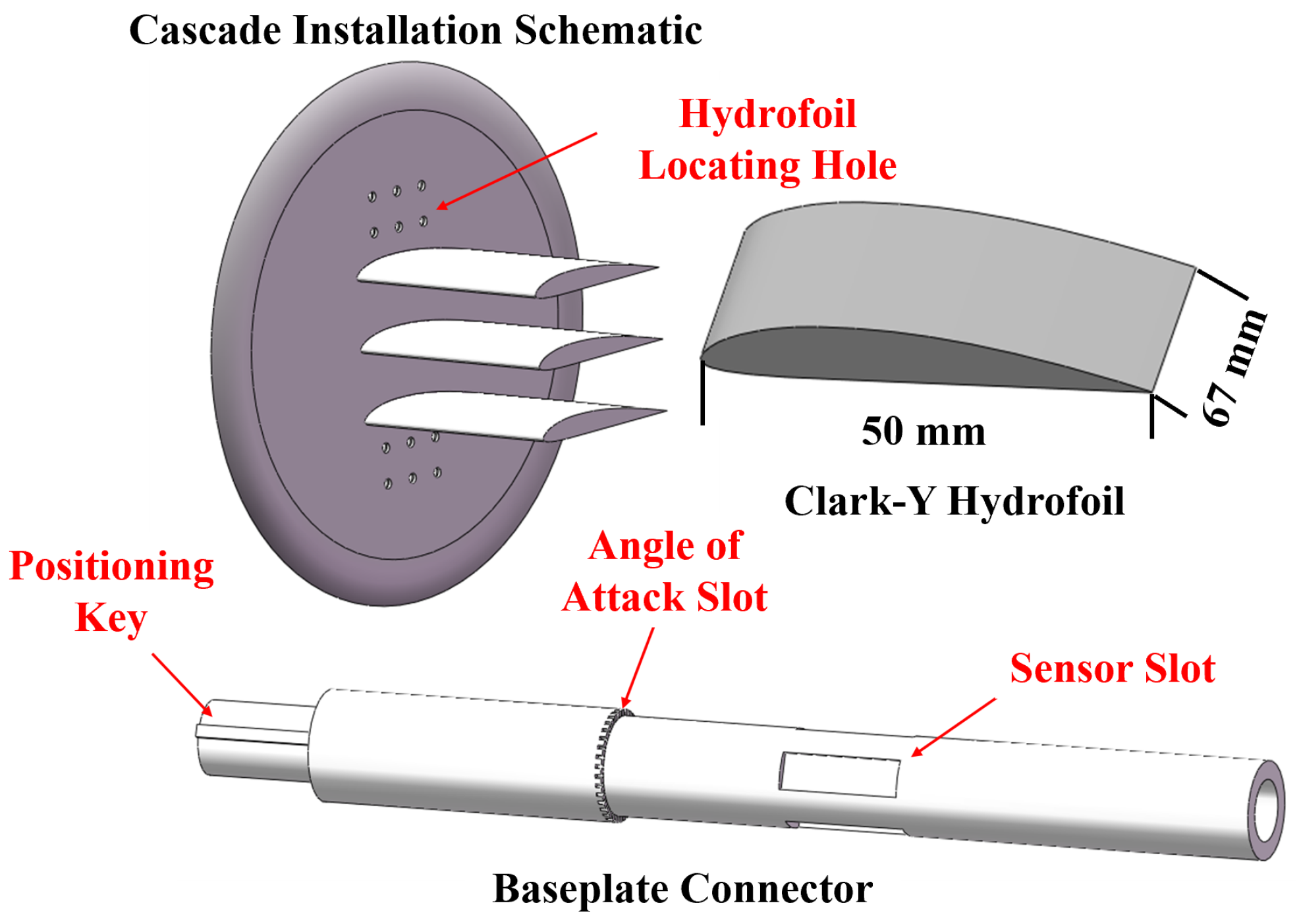
The cascade used in the experiment consisted of three Clark-Y hydrofoils, as shown in Figure 2, with a chord length (C) of 50 mm and a span (S) of 67 mm. To ensure stable installation within the test section of the water tunnel, the hydrofoils were connected via large circular baseplates, the edges of which featured a rounded design to minimize any interference with the cavitation development on the hydrofoils. A total of 36 slots were machined at the fixed end of the test section, with each slot corresponding to a 10° increment, allowing for precise control of the model’s angle of attack (AOA). To ensure the coaxiality of the entire assembly, positioning keys and holes were integrated into the hydrofoils, baseplates, and connectors. All models were fabricated using 3D printing technology with stainless steel, achieving a surface roughness of Ra 3.2 to ensure that the cavity flow remained unaffected by surface irregularities.

2.1.3. PIV Velocity Field Measurement System

To further investigate the influence of the cascade structure on the internal flow field, a non-intrusive Particle Image Velocimetry (PIV) measurement system was introduced in this study. The system utilizes a laser sheet to illuminate the flow field seeded with tracer particles, followed by a correlation analysis of the recorded particle images to derive the velocity vectors. The intermediate results of each stage during the PIV measurement process are illustrated in Figure 3. Specifically, the PIV system comprises a Vlite Hi 527-25 (Beamtech Optronics Co., Ltd., Beijing, China) laser source, a cross-frame high-speed camera, and hollow glass microspheres with diameters ranging from 20 to 50 µm as tracer particles. An optical filter with a center wavelength of 532 ± 2 nm was employed to eliminate interference from background reflections. During the experiment, a dedicated workstation running the PIV control and processing software, DynamicStudio V8.4, was used to calculate the flow velocity based on the preset time intervals and the particle displacement extracted from the synchronized images.

2.2. Numerical Calculation Method

2.2.1. Turbulence Model

Turbulence remains one of the greatest unsolved challenges of the 21st century, leading scholars to propose various simulation equations [25,26,27]. Among these, Large Eddy Simulation (LES) has emerged as a high-precision model and is increasingly adopted by the research community. Its accuracy lies in its approach to decomposing the vortices in the flow field into large- and small-scale components [28,29,30]. Specifically, large-scale eddies are solved directly using Navier–Stokes (N-S) equations, while the effects of small-scale eddies are captured through sub-grid scale (SGS) stress terms. Consequently, LES offers superior solution accuracy compared to conventional Reynolds-Averaged Navier–Stokes (RANS) models. Its primary governing equations are as follows:
ρ m u i ¯ t + ρ m u i ¯ u j ¯ x j = p ¯ x i + x j μ m u i x j + u j x i + τ i j x j
where ρ m is the density of the mixture medium, u i is the velocity component, x i denotes the Cartesian coordinates ( i = 1 , 2 , 3 ), p is the static pressure, and τ i j is the sub-grid scale (SGS) stress, which describes the influence of small-scale eddies. Its expression is defined as
τ i j = ρ m u i u j ¯ u ¯ i u ¯ j
Large-scale eddies are solved directly using the filtered N-S equations, while small-scale eddies are calculated using the Wall-Adapting Local Eddy-viscosity (WALE) stress model, as detailed below:
τ i j 1 3 δ i j τ k k = 2 μ t S i j ¯
S i j ¯ = 1 2 u i ¯ x j + u j ¯ x j
where δ i j is the Kronecker delta ( δ i j = 1 if i = j , and δ i j = 0 if i j ), i , j denote the Cartesian coordinate directions, S i j ¯ is the large-scale resolved strain rate tensor, and τ k k is the isotropic component of the sub-grid scale (SGS) stress tensor. In Large Eddy Simulation (LES), μ t represents the turbulent viscosity specifically for small-scale eddies. The total dynamic viscosity μ t used in the calculation model is defined as follows:
μ t = ρ L S 2 S i j d S i j d 3 / 2 S ¯ i j S ¯ i j 5 / 2 + S i j d S i j d 5 / 4
L S = min κ d , C w V 1 / 3
S i j d = 1 2 g ¯ i j 2 + g ¯ j i 2 1 3 δ i j g ¯ k k 2
g i j = u i ¯ x j
where d represents the distance from the grid to the nearest boundary, V is the local grid volume, κ is the Karman constant with a value of 0.4, and C w is the WALE model constant set to 0.325. The WALE model employs a zero-eddy-viscosity approach in laminar shear layers, which allows for a superior description of the cavity shedding phenomena within the hydrofoil boundary layer.

2.2.2. Cavitation Model

As cavitation occurs within the cascade flow field, it is essential to incorporate a cavitation model into the numerical simulation. This study employs the Zwart–Gerber–Belamri (Z-G-B) model [31], which describes the phase change process based on a volume fraction transport equation and has demonstrated excellent robustness in simulating unsteady cavitating flows. By employing Large Eddy Simulation (LES), it is still possible to effectively capture large-scale cavity shedding and the resulting pressure waves. The Z-G-B model assumes that all bubbles in the fluid have a uniform size. It utilizes the bubble number density (n) and mass change rate of a single bubble to characterize the interphase mass transfer rate per unit volume R:
R = n × 4 π R B 2 ρ v D R B D t
where R B is the bubble radius (taken as 1 × 10 6 m), and ρ v is the vapor density. The relationship between the vapor volume fraction, bubble number density, and bubble radius is expressed as follows:
α = n × 4 3 π R B 3
By substituting the above two equations, the following can be obtained:
R = 3 α ρ v R B 2 3 P B P ρ l
where P B denotes the pressure at the bubble surface, P represents the local far-field pressure (or local fluid pressure), and ρ l is the liquid density. To further describe the process of bubbles collapsing back into the liquid phase, the aforementioned equations are generalized as follows:
R e = F 3 α ρ v R B 2 3 P B P ρ l si g n P B P
where R e represent the evaporation source terms, and F is an empirical constant derived from the evaporation process, which differs from the value used for condensation. A key assumption of this equation is that there are no intense interactions between bubbles; thus, it is only applicable to the early stages of cavitation. However, during the violent shedding stage, the bubble nuclei density increases. Consequently, the final governing equations for the Z-G-B model are expressed as follows:
Evaporation ( p < p v ):
R e = F v a p 3 α n u c ( 1 α v ) ρ v R B 2 3 P v P ρ l
Condensation ( p > p v ):
R c = F c o n d 3 α v ρ v R B 2 3 P P v ρ l
where P v is the saturation vapor pressure, R c denotes the condensation source terms, α n u c is the volume fraction of the bubble nuclei, F v a p is the evaporation coefficient set to 50, and F c o n d is the condensation coefficient set to 0.01.

2.3. Numerical Model and Validation

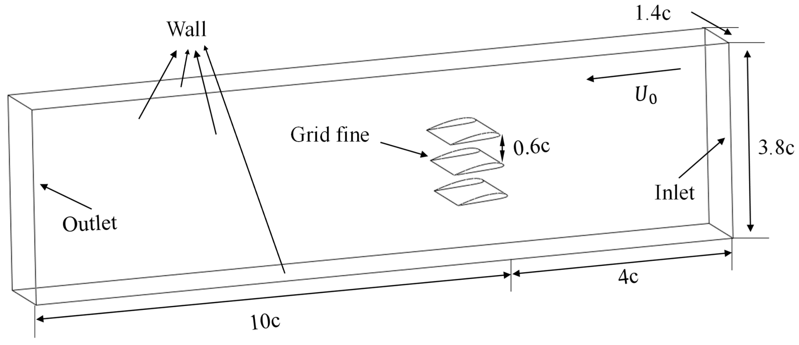
The computational model and boundary conditions established in this study are illustrated in Figure 4. The model dimensions and operating conditions are consistent with the experimental setup, featuring a hydrofoil chord length of C = 50 mm and an angle of attack (AOA) of 8 . The computational domain is a rectangular region with dimensions of 14 C in length, 3.8 C in height, and 1.4 C in width, which matches the test section of the water tunnel. The governing equations were solved using the pressure-based solver in Ansys Fluent 2023 R1. The boundary conditions were configured as a velocity inlet and pressure outlet. The remaining boundaries were set as wall conditions. The inlet velocity was primarily set at 8 m/s, and the cavitation intensity within the domain was regulated by adjusting the inlet velocity and outlet pressure. The cavitation degree is characterized by the dimensionless cavitation number σ , as defined in Equation (15). According to the turbulence intensity formula I = 0.16 × ( R e D ) 1 / 8 , the boundary turbulence intensity is approximately 2.7%. Both the hydrofoil surfaces and domain boundaries were set as adiabatic, no-slip walls. Based on non-dimensional parameters and the Large Eddy Simulation (LES) framework, the model is theoretically applicable to hydrofoils of other dimensions within a similar flow regime.
To provide a clearer description of the flow field information surrounding the cascade, the lift and drag coefficients are defined in Equations (16) and (17), respectively.
σ = P P o u t 0.5 ρ l U 0 2
C L = F L 0.5 ρ l U 0 2 S C
C d = F d 0.5 ρ l U 0 2 S C
where P is the atmospheric pressure, P o u t is the outlet pressure, and U 0 is the inlet velocity. F L and F d denote the lift and drag forces acting on the hydrofoil, respectively. ρ l represents the water density, while S and C denote the span and chord length of the hydrofoil, respectively.
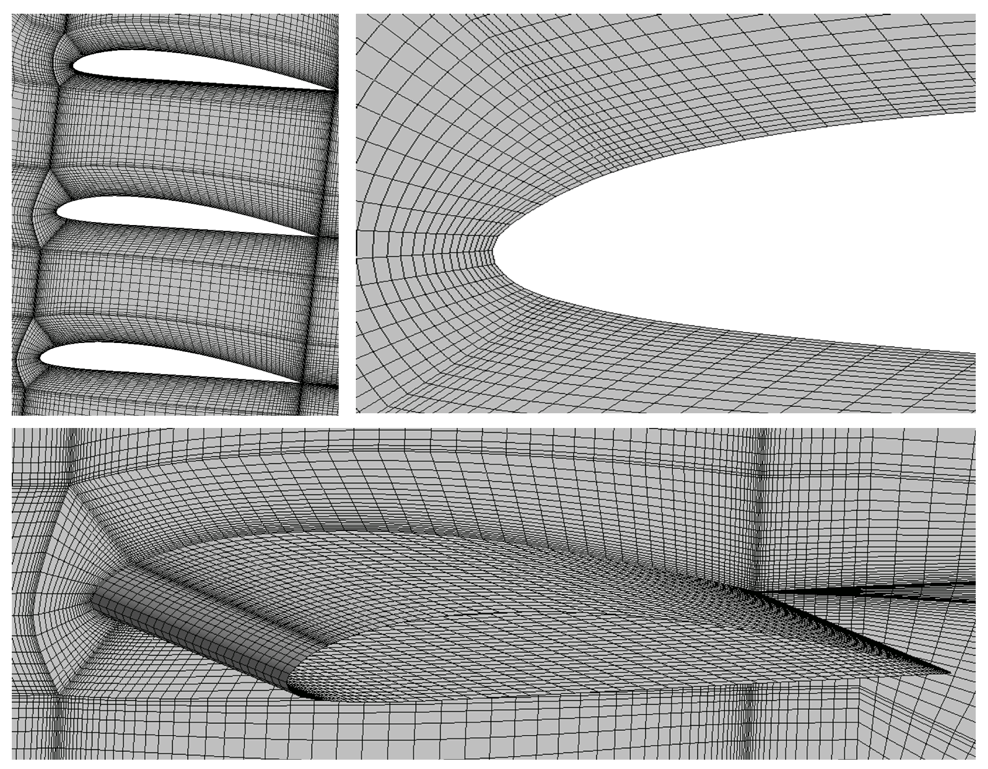
Figure 5 illustrates the mesh generation for the cascade. To effectively capture small-scale eddies, Large Eddy Simulation (LES) requires high-quality grid distribution. Consequently, in this study, ICEM 2023 R1 software [32] was utilized to generate hexahedral structured meshes, with local refinement applied to the hydrofoil boundary layers. This refinement was designed to accurately capture the cavity shedding process from the hydrofoil surface and extract the re-entrant jet phenomenon. Furthermore, to satisfy the requirements of the LES wall function, the y + value on the hydrofoil surface was maintained below 1, thereby ensuring the capture of fine cavitating structures.
To eliminate the influence of grid density on the flow field around the cascade, a mesh independence study was conducted. Taking the cascade at an 8 angle of attack (AOA) and a flow velocity of 8 m/s as the benchmark case, simulations were performed to extract the lift and drag coefficients, and the results are summarized in Table 1. As the number of grid nodes increases beyond 3 million, the lift coefficient gradually stabilizes. When the mesh count reaches over 5 million, both the lift and drag coefficients remain essentially constant. Therefore, a total grid count of 4.76 million was selected for the computational domain in this study.
To eliminate the influence of time-step size on the computational results, independence verification was conducted for five different time steps, as summarized in Table 2: 1 × 10 3 s, 5 × 10 4 s, 1 × 10 4 s, 5 × 10 5 s, and 1 × 10 5 s. The total mesh count was fixed at 4.76 million. The simulation results indicate that an excessively large time step leads to significant deviations in the lift and drag coefficients. When the time step is reduced below 5 × 10 5 s, the results tend to converge. Consequently, 5 × 10 5 s was selected as the time step for the actual numerical simulations.
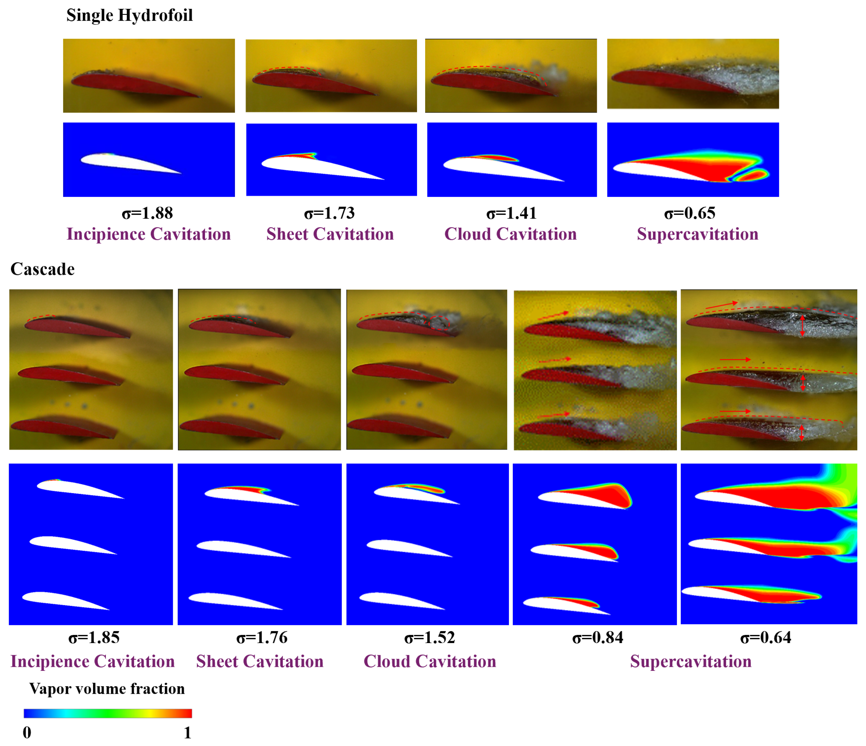
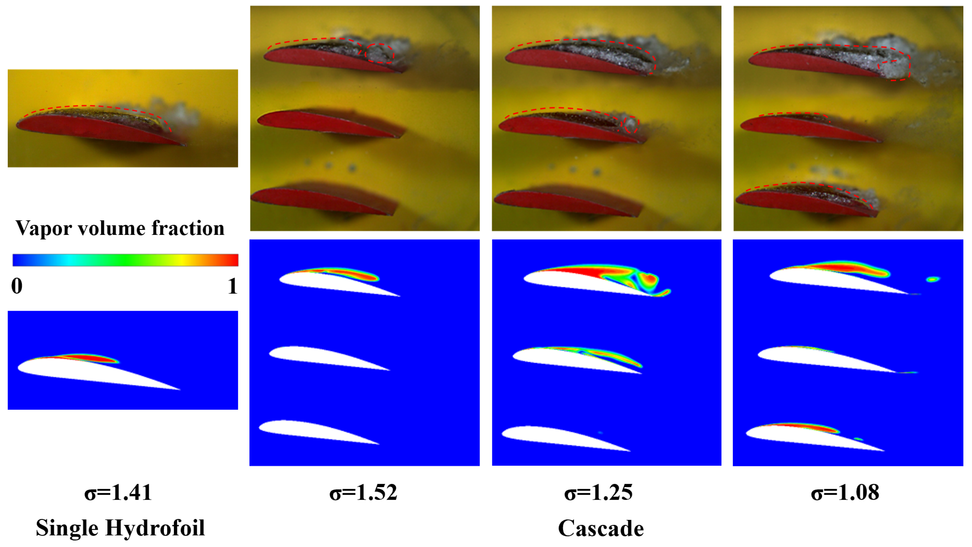
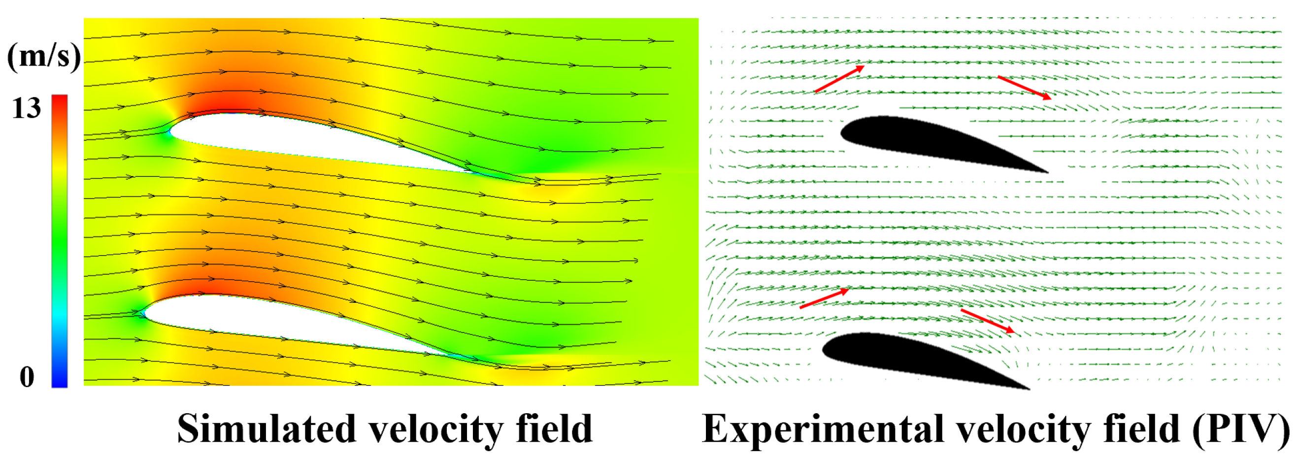
To verify the accuracy of the numerical results, Figure 6 compares the experimental observations and numerical snapshots of the flow around a single hydrofoil and the cascade under various cavitation numbers. The comparison reveals that the cavity boundaries, represented by the vapor volume fraction in the numerical results, are in excellent agreement with the gas–liquid interfaces observed in the experiments. Figure 7 presents the velocity fields around the cascade obtained from both numerical simulations and Particle Image Velocimetry (PIV) measurements. It can be observed that while the water flow moves upward upon encountering the hydrofoil leading edge, the flow around the middle hydrofoil of the cascade is influenced by the suction side of the top hydrofoil, causing it to move directly downstream with a significantly reduced upward displacement. The numerical results clearly reflect these flow trajectories. Furthermore, the relative errors ( E r e l ) between the experimental and simulated relative error of the cavity area across all operating conditions were calculated and are summarized in Table 3. The relative error is defined as the ratio of the absolute difference between the numerical and experimental results to the experimental value, as shown in Equation (18). Notably, all errors remain below 5%. In summary, the proposed numerical method for unsteady cavitating flow around a cascade can accurately predict the cavity evolution and flow field characteristics.
E r e l = | α v , C F D α v , E X P | α v , E X P × 100 %

3. Results and Discussion

3.1. Evolutionary History of Unsteady Cavitation in the Cloudy Cavitation Phase of Cascade

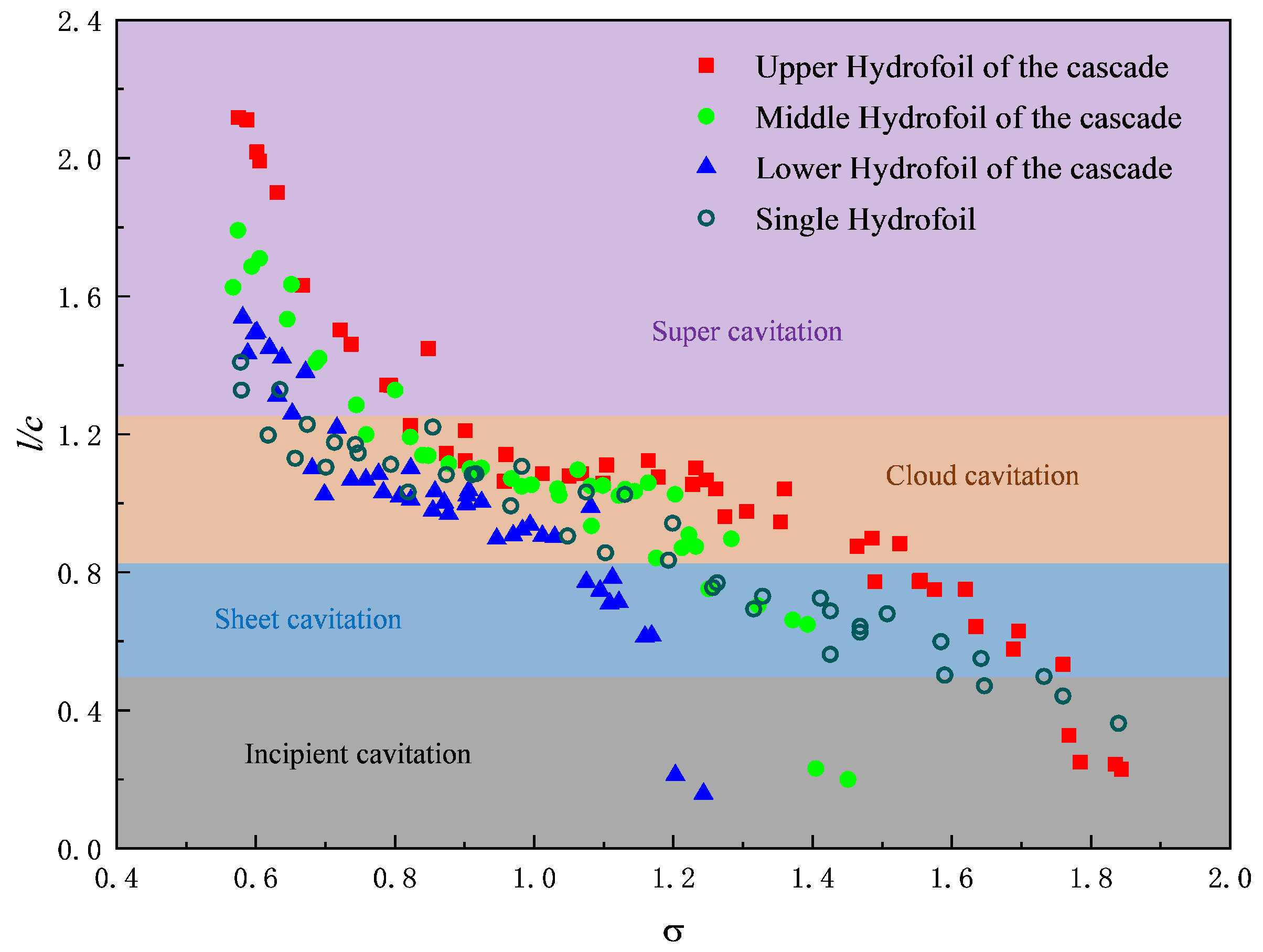
Figure 8 presents the cavity morphologies around a single hydrofoil and the cascade at various cavitation stages with an 8 angle of attack. The comparison reveals that cavitation inception occurs around the single hydrofoil at σ 1.88 . As the cavitation number decreases to σ 1.85 , cavitation begins to appear at the leading edge of the top hydrofoil in the cascade, while no cavitation is observed around the middle and bottom hydrofoils. During this inception stage, the flow phenomena around the top hydrofoil and the single hydrofoil are similar. At σ 1.76 , the top hydrofoil enters the sheet cavitation stage, followed by the single hydrofoil at σ 1.73 , showing a high similarity in sheet cavity morphology between the two flow fields. However, cavity development differs significantly across various positions within the cascade; compared to the top hydrofoil, cavitation is more difficult to trigger around the middle and bottom hydrofoils. When σ 1.52 , the top and middle hydrofoils are in the cloud and sheet cavitation stages, respectively, whereas the bottom hydrofoil remains cavitation-free. As σ drops to 1.41, the single hydrofoil enters the cloud cavitation stage, maintaining the sheet cavitation phase for a longer duration than the top hydrofoil. At σ 0.84 and σ 0.8 , the flow around the top and middle hydrofoils enters the super-cavitation stage, with the cavity at the trailing edge of the top hydrofoil tending to move upward. When the cavitation number further decreases to σ 0.64 , both the single hydrofoil and the bottom hydrofoil enter the super-cavitation stage, at which point all hydrofoils in the cascade are in the super-cavitation regime. In comparison, the cavitation stages for the single hydrofoil persist over a wider range of cavitation numbers. Due to the influence of the cascade structure on the middle and bottom hydrofoils, the cavities tend to develop toward the trailing edge, resulting in a shortened cloud cavitation stage.
The previous section described the differences in cavity morphology between the single hydrofoil and the cascade across various cavitation stages. To further elucidate the flow field variations among the individual hydrofoil layers within the cascade, Figure 9 presents the profiles of the maximum relative cavity length as a function of the cavitation number. The maximum relative cavity length is defined as the ratio of the maximum cavity length to the hydrofoil chord length. It can be observed from the figure that the cavitation stages for the single hydrofoil and top hydrofoil of the cascade persist over a wider range compared to the middle and bottom layers, with the single hydrofoil exhibiting the broadest range. In the flow fields of the middle and bottom hydrofoils, cavities detach more easily from the wall and develop toward the trailing edge; this accelerated cavity growth leads to a contraction of their respective cavitation stages. During the cloud cavitation stage, the maximum cavity length of the middle hydrofoil gradually surpasses that of the top hydrofoil. In the super-cavitation stage, the cavity length of the top hydrofoil is significantly greater than those of the middle and bottom layers. At this point, the cavity length exceeds the chord length, and the influence of the cascade structure diminishes, resulting in a decelerated cavity development rate for the middle and bottom hydrofoils. In summary, the cavity development pattern of the top hydrofoil follows that of the single hydrofoil but at a higher growth rate. Conversely, the middle and bottom hydrofoils experience weakened cavitation intensity due to the cascade structure; however, their accelerated cavity development and shortened cloud cavitation stage help mitigate the cavitation erosion caused by periodic cavity collapse on the hydrofoil surface.
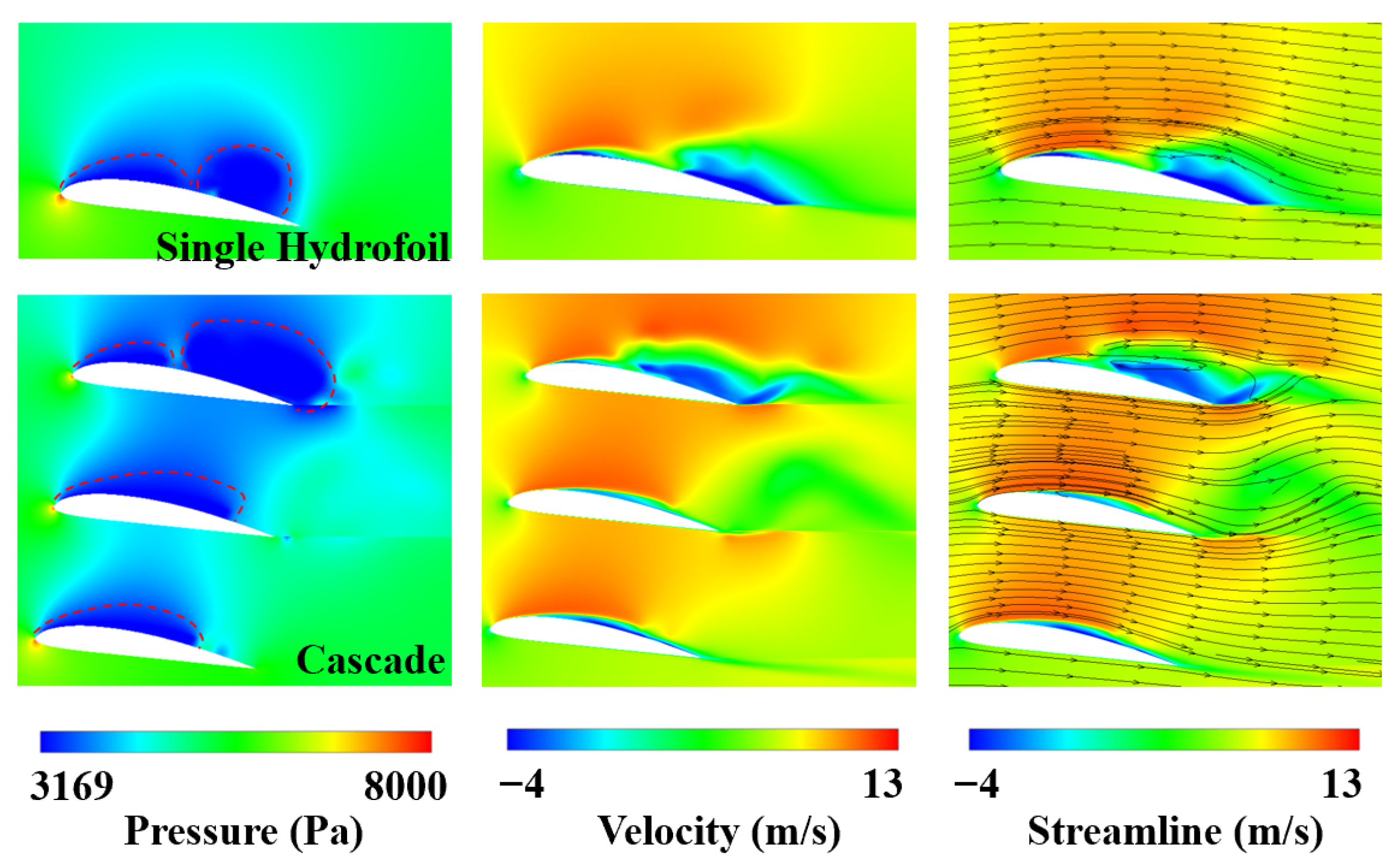
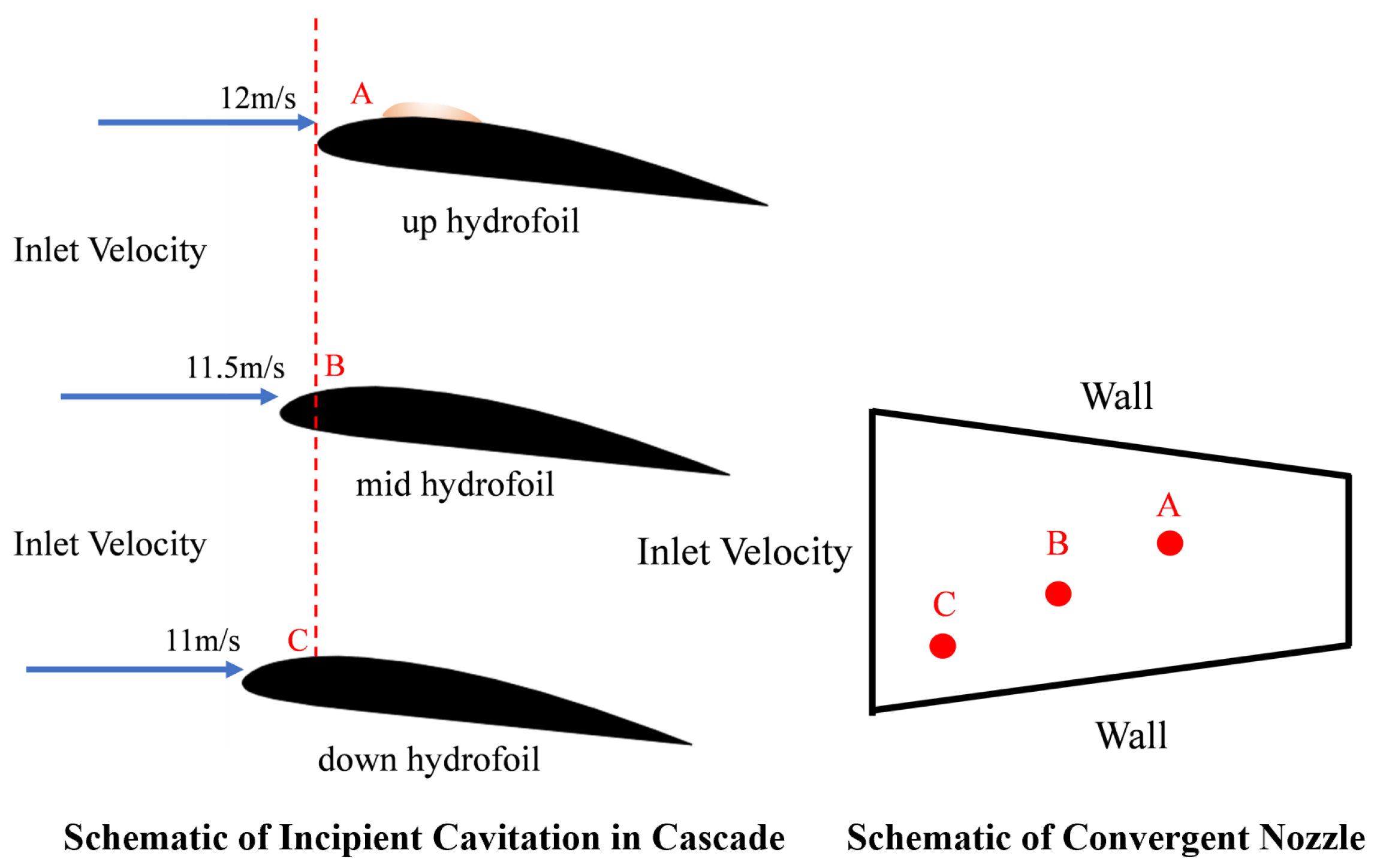
In summary, the study of the flow characteristics around the single hydrofoil and cascade across different cavitation stages reveals that the primary differences lie in the following aspects: compared to the single hydrofoil and top hydrofoil, cavitation within the cascade occurs later, and its intensity is less severe. To further investigate the influence of the cascade structure on cavitation characteristics, the pressure contours, velocity contours, and streamlines at σ = 1.5 are extracted, as shown in Figure 10. The pressure contours indicate that the internal pressure field of the cascade is influenced by the suction side of the top hydrofoil, which prevents the low-pressure region from extending upward, leading to a more uniform pressure distribution. When the re-entrant jet in the top hydrofoil flow field reaches the mid-chord, the attached cavity breaks, causing the low-pressure region on the foil surface to split into two parts. From the velocity contours, the larger scale of the re-entrant jet in the single and top hydrofoil flows leads to a greater upward displacement of the trailing-edge cavity, resulting in the formation of large-scale shedding cavities. Due to the cascade effect, the high-velocity regions around the middle and bottom hydrofoils are closer to the foil surface, and the re-entrant jet is less pronounced. The streamlines further demonstrate that the upward movement of the fluid is restricted by the suction side of the top hydrofoil, forcing the internal streamlines closer to the hydrofoil surface. Additionally, as shown in Figure 11, when the cascade rotates at a specific angle of attack, the leading edges of the hydrofoils are not vertically aligned, resulting in variations in the leading-edge flow velocity. Observations at the inception stage ( σ = 1.85 ) show that the inflow velocity is not constant across the layers but gradually decreases from top to bottom. The relative positions of the leading edges can be compared to various sections of a converging nozzle. As indicated by points A, B, and C, according to the area–velocity relationship for subsonic flow in a converging nozzle, the flow velocity increases and pressure decreases as the cross-sectional area reduces. Consequently, to maintain the angle of attack, the inflow velocity decreases progressively from the top to the bottom layer. Therefore, cavitation is most intense on the top hydrofoil and weakens in subsequent layers.

3.2. Unsteady Cavity Collapse Mechanism at the Cloudy Cavitation Stage of the Cascade

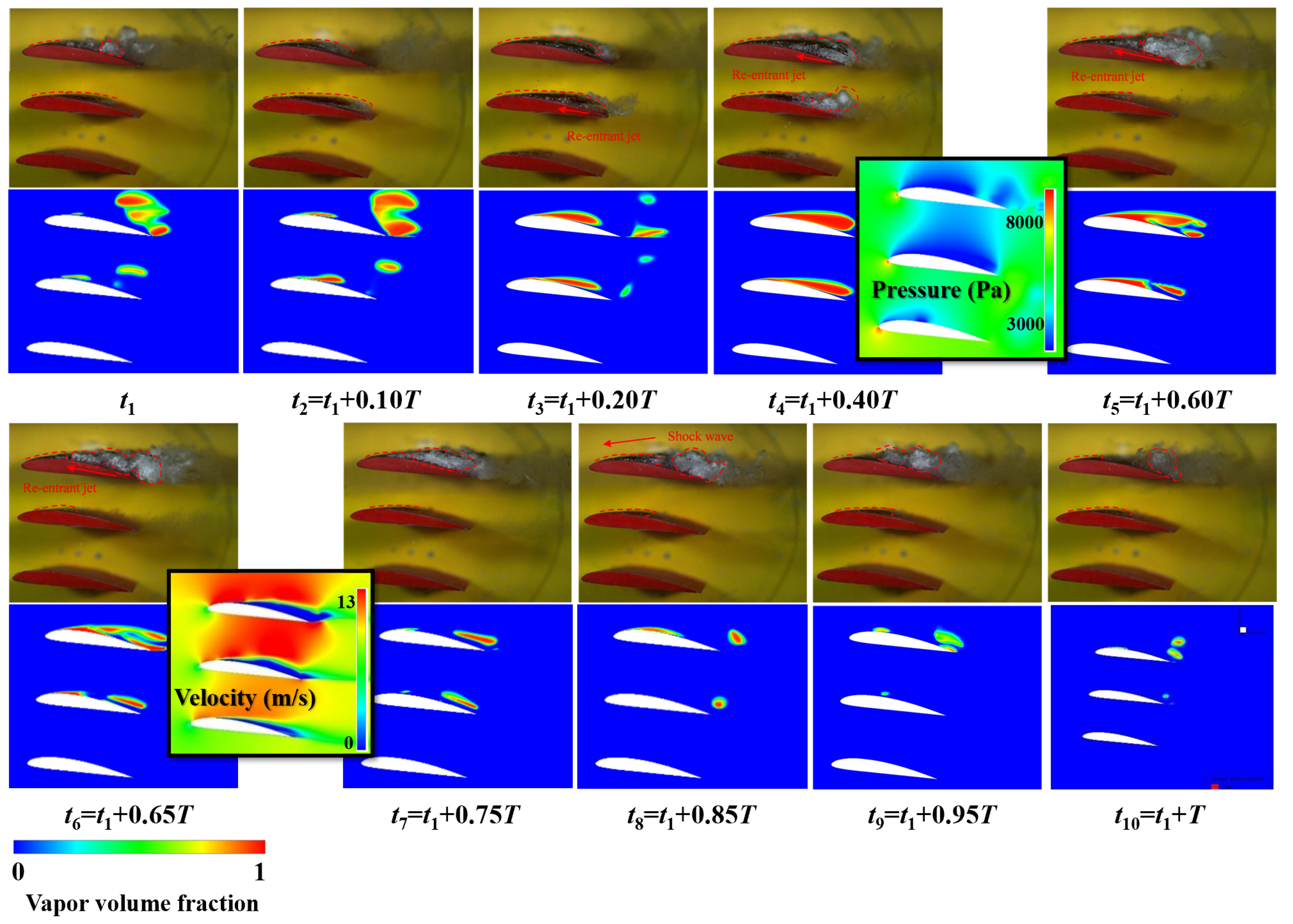
The previous section detailed the cavitation characteristics of the flow around the cascade and single hydrofoil at various stages. Given the significant hazards associated with quasi-periodic cloud cavitation, this section focuses on the cavity collapse mechanisms during the cloud cavitation stage. Figure 12 illustrates the unsteady cavity evolution around each hydrofoil layer of the cascade at σ = 1.24 . At t = t 1 , a cavity emerges at the leading edge of the top hydrofoil, while a large-scale vapor cloud from the previous cycle remains partially uncollapsed at its trailing edge. By t = t 3 , this trailing-edge cloud has collapsed completely, and a re-entrant jet phenomenon begins to appear in the flow around the middle hydrofoil. From t = t 4 to t 5 , a re-entrant jet develops in the downstream region of the top hydrofoil and advances toward the leading edge; its interaction with the main flow causes a large-scale cloud to shed from the trailing edge. In contrast, due to the lower intensity of the re-entrant jet on the middle hydrofoil, only small-scale vapor structures shed from its trailing edge, causing its attached cavity to collapse toward the leading edge. The pressure contours reveal that the low-pressure area above the middle hydrofoil is larger than that of the top layer, resulting in a longer attached cavity. At t = t 6 , the re-entrant jet on the top hydrofoil reaches the leading edge, leading to cavity breakage and large-scale shedding. At this point, the middle hydrofoil cavity has collapsed back to the leading edge and initiates a new cycle. The velocity contours clearly show that the scale of the re-entrant jet on the middle hydrofoil is significantly smaller than that on the top hydrofoil. From t = t 7 to t 8 , the top hydrofoil begins a new cycle; the high vapor content and large scale of the shed clouds release substantial energy upon collapse, generating shock wave phenomena. At t = t 9 , the shock waves produced by the collapsing clouds cause the nascent attached cavity to collapse before it can reach the trailing edge—a process identified as the shock-induced collapse mechanism. Meanwhile, the middle hydrofoil cavity continues to develop toward the trailing edge. By t = t 10 , the top hydrofoil commences another cycle of cavity growth. In summary, the cavity collapse periods are inconsistent across different hydrofoil positions within the cascade, with the top hydrofoil exhibiting more intense cavitation and a longer period. Furthermore, the collapse mechanisms vary: the flow around the top hydrofoil is characterized by prominent re-entrant jets and shock wave mechanisms, whereas the middle hydrofoil is primarily governed by the re-entrant jet mechanism.
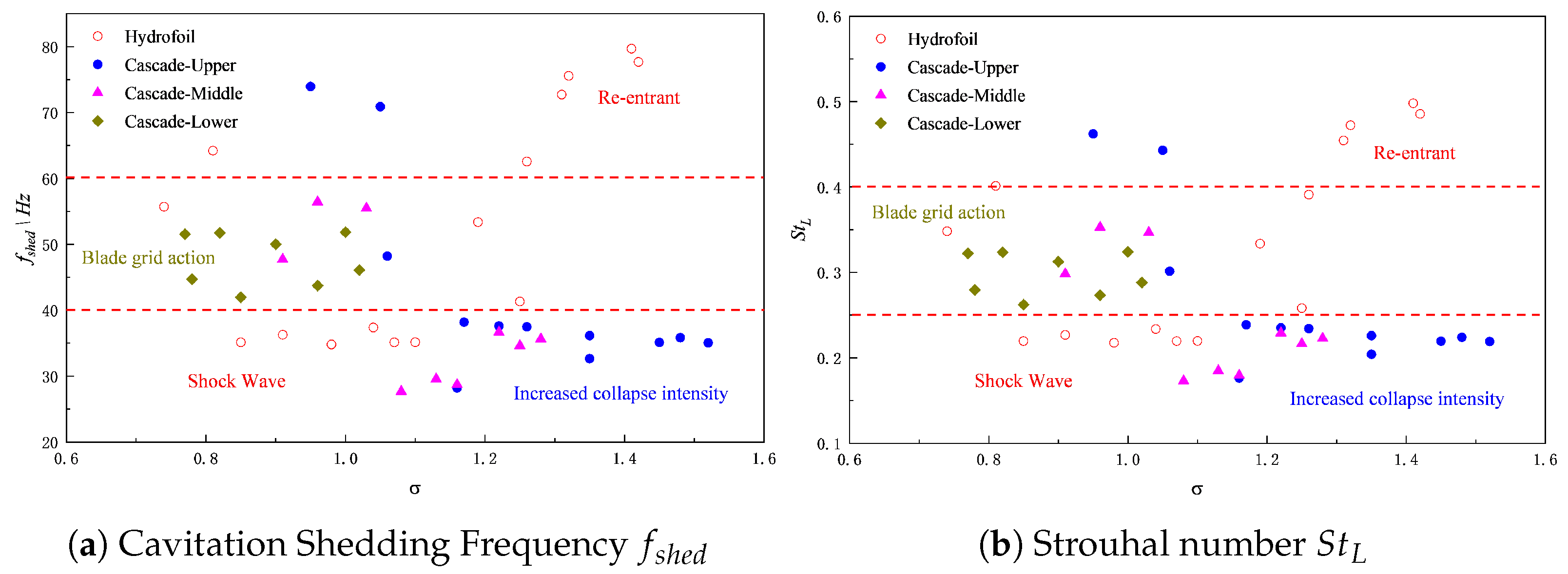
To further compare the periodicity of cavity shedding between the single hydrofoil and cascade during the cloud cavitation stage, Figure 13 illustrates the variation in cavity shedding frequency ( f s h e d ) and Strouhal number ( S t L ) as a function of the cavitation number across different flow field positions. The cavity shedding frequency is taken as the average value obtained from the experimental results of the unsteady cavitating flow around the cascade. The Strouhal number, a dimensionless representation of the shedding frequency, is defined as follows:
S t L = f shed L U
As illustrated in Figure 13, the distribution of cavity shedding frequency and Strouhal number ( S t ) for the single hydrofoil exhibits distinct stage-wise characteristics. The Strouhal numbers range between 0.2 and 0.45, which is attributed to the coexistence of two collapse mechanisms in the cloud cavitation stage—the re-entrant jet and shock-induced mechanisms—corresponding to shedding frequencies of 0.45 and 0.2, respectively. Compared to the re-entrant jet mechanism, the shock-induced mechanism involves two cavity growth phases; in the second phase, the cavity collapses rapidly under the influence of the large-scale shed vapor cloud from the previous cycle, thereby reducing the shedding frequency. As previously discussed, the flow around the top hydrofoil of the cascade also exhibits both collapse mechanisms. However, due to the accelerated cavity development in the cascade, the flow field enters the shock-induced regime more quickly, resulting in Strouhal numbers for the top hydrofoil primarily clustered around 0.2. Influenced by the cascade structure, the flow fields around the middle and bottom hydrofoils remain relatively stable, making cavity collapse more difficult. Specifically for the bottom hydrofoil, cavity collapse occurs predominantly at the trailing edge with a longer cycle and a more stable mechanism, maintaining a Strouhal number of approximately 0.3. The cavitation intensity of the middle hydrofoil lies between that of the top and bottom layers. At the onset of cloud cavitation, its Strouhal number is consistent with the top hydrofoil at approximately 0.2. As the cavitation number further decreases, the cavities around the middle hydrofoil can no longer collapse completely, and its Strouhal number aligns with that of the bottom hydrofoil at approximately 0.3.

3.3. Analysis of Dynamic Characteristics of Unsteady Flow Around a Cascade

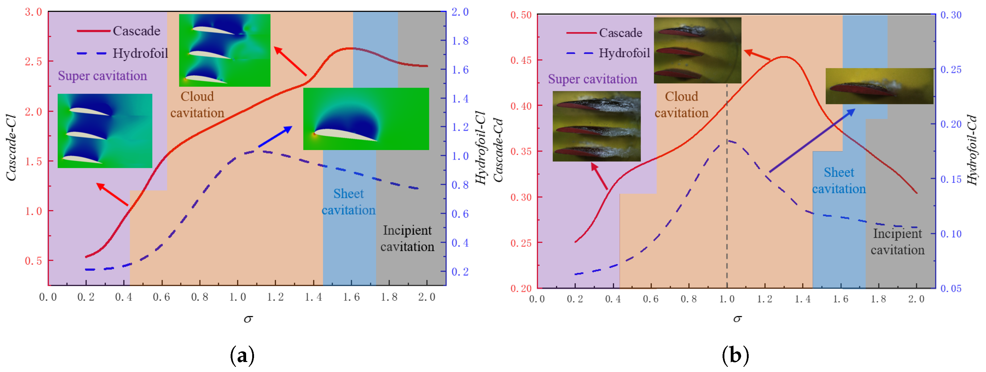
The preceding sections clarified the unsteady cavitation characteristics of the flow around a single hydrofoil and cascade across different stages as well as the cavity collapse mechanisms for each hydrofoil layer during the cloud cavitation stage. This section further explores the dynamic characteristics of the unsteady flow around the cascade. Figure 14a illustrates the variation in lift coefficients ( C L ) for the single hydrofoil and cascade as a function of the cavitation number. It can be observed that the lift performance of the cascade is significantly superior to that of the single hydrofoil. However, during the late cloud cavitation and super-cavitation stages, the lift of the cascade drops sharply, with a decline rate considerably higher than that of the single hydrofoil. Between σ = 1.7 and 2.1 , both configurations are in the non-cavitating or incipient cavitation stages, where cavitation does not significantly impact the lift. During this phase, the C L for the cascade and single hydrofoil is 1.8 and 0.6, respectively, indicating that the cascade lift is three times that of the single hydrofoil. As σ decreases, both enter the sheet cavitation stage. The cavities attached to the leading edge increase the effective curvature of the hydrofoil and reduce the suction-side pressure while the pressure side remains unaffected, further enhancing the lift coefficients. Between σ = 0.8 and 1.4 , both are in the cloud cavitation stage. As discussed in Section 3.1, the duration of each cavitation stage is shorter for the cascade. Consequently, the cascade’s C L reaches its peak rapidly at the onset of cloud cavitation and then declines sharply. With a further decrease in σ , while the pressure-side pressure remains at the saturated vapor pressure (3169 Pa), the suction-side pressure continues to decrease, causing the lift to drop. At σ = 1.35 , a low-pressure region emerges between the top and middle hydrofoils, reducing the lift contribution from the top layer and causing a continuous decline in the total C L . Beyond σ = 0.6 , the cavity on the single hydrofoil extends to the trailing edge and stabilizes, leading to a gradual reduction and stabilization of its C L in the super-cavitation stage, whereas the cascade’s C L drops to approximately 0.5.
While providing higher lift, the cascade also incurs increased drag. Figure 14b shows the variation in drag coefficients ( C d ) with the cavitation number. At high cavitation numbers, the cascade’s C d is also three times that of the single hydrofoil. As σ decreases, cavities appear at the leading edge of the pressure side and expand toward the trailing edge, causing the drag for both to increase simultaneously and peak during the cloud cavitation stage, following a trend similar to the lift coefficient. Compared to the single hydrofoil, the cascade’s C d reaches its maximum earlier before declining. At σ = 1.0 , the cascade’s C d is twice that of the single hydrofoil. In the super-cavitation stage, the C d for both reaches a minimum, at which point the cascade’s minimum drag is approximately three times that of the single hydrofoil.
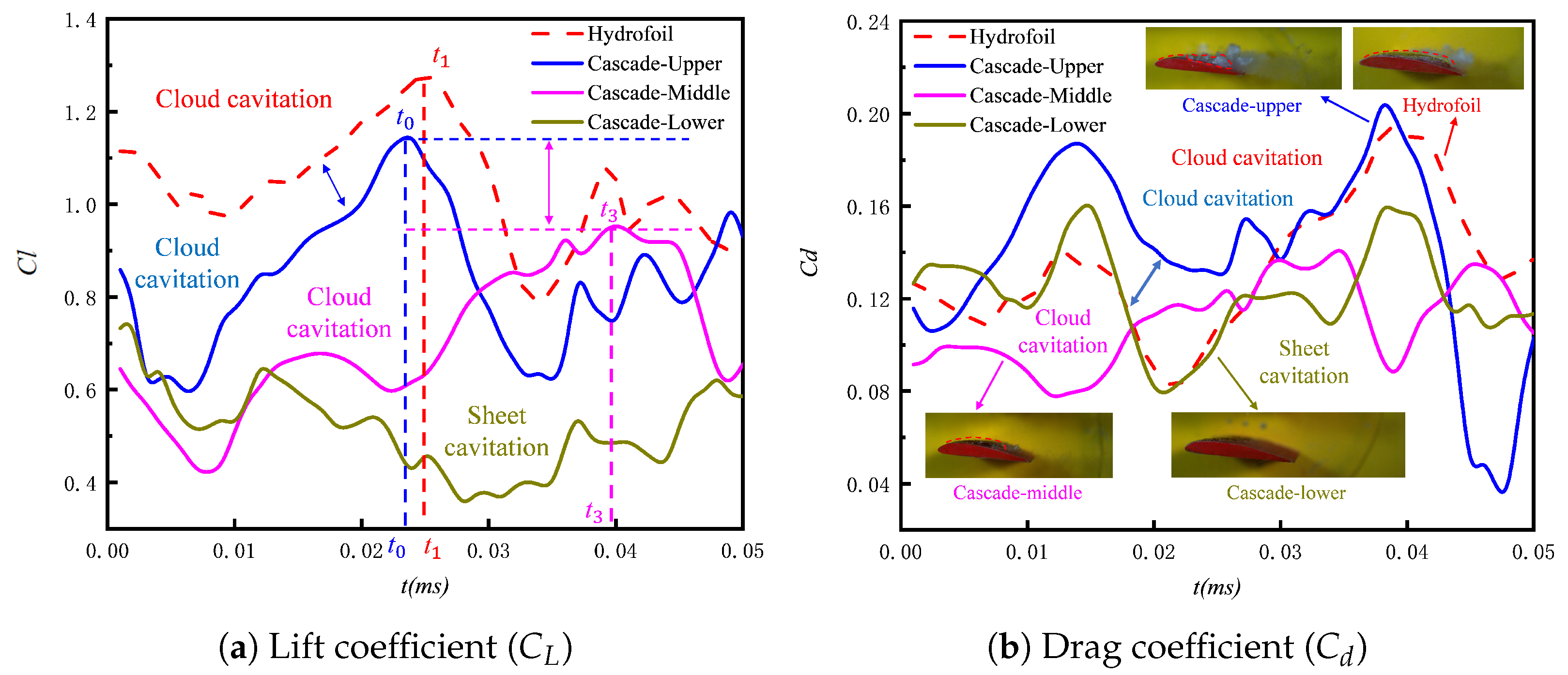
As established in the previous section, the lift performance of the cascade is significantly superior to that of the single hydrofoil, but it also incurs substantially higher drag. During the cloud cavitation stage, the cavitation process within the cascade is unsteady and periodic; therefore, characterizing the entire process using time-averaged lift and drag coefficients is insufficient. Figure 15 illustrates the time-resolved drag coefficients for the single hydrofoil and each layer of the cascade at σ = 1.24 (the cloud cavitation stage). Regarding the lift coefficients, the variation pattern of the top hydrofoil aligns with that of the single hydrofoil, although the single hydrofoil exhibits higher absolute values. Due to the distinct cavity evolution patterns across the cascade layers, the lift coefficient fluctuations vary among the hydrofoils. Specifically, the top hydrofoil provides higher lift during the middle of the cycle, whereas the middle hydrofoil delivers greater lift during the middle-to-late stages. This is attributed to the lower pressure within the internal flow field of the cascade; conversely, the bottom hydrofoil, which lacks significant cavitation, maintains higher flow field pressure. This results in higher suction-side pressure for the middle hydrofoil, thereby enhancing its lift performance relative to the top layer. The bottom hydrofoil remains in the sheet cavitation stage, thus exhibiting no pronounced lift peaks and contributing less total lift than the upper two layers.
The drag coefficient profiles indicate that the drag on the top hydrofoil is markedly higher than that on the single hydrofoil, despite providing less lift. The reduction in lift for the top hydrofoil is caused by a decrease in the pressure difference between its pressure and suction sides, as the suction-side pressure drops while the pressure-side remains consistent with the single hydrofoil case. As previously noted, the fluid passing the leading edge of the middle hydrofoil initially moves upward before being diverted horizontally downstream by the influence of the top hydrofoil’s suction side. This phenomenon increases the drag on the top hydrofoil, causing its lift-to-drag performance to fall below that of the single hydrofoil. Consequently, regarding the drag characteristics of the cascade, optimization of the top hydrofoil design could potentially reduce drag while maintaining the required lift.
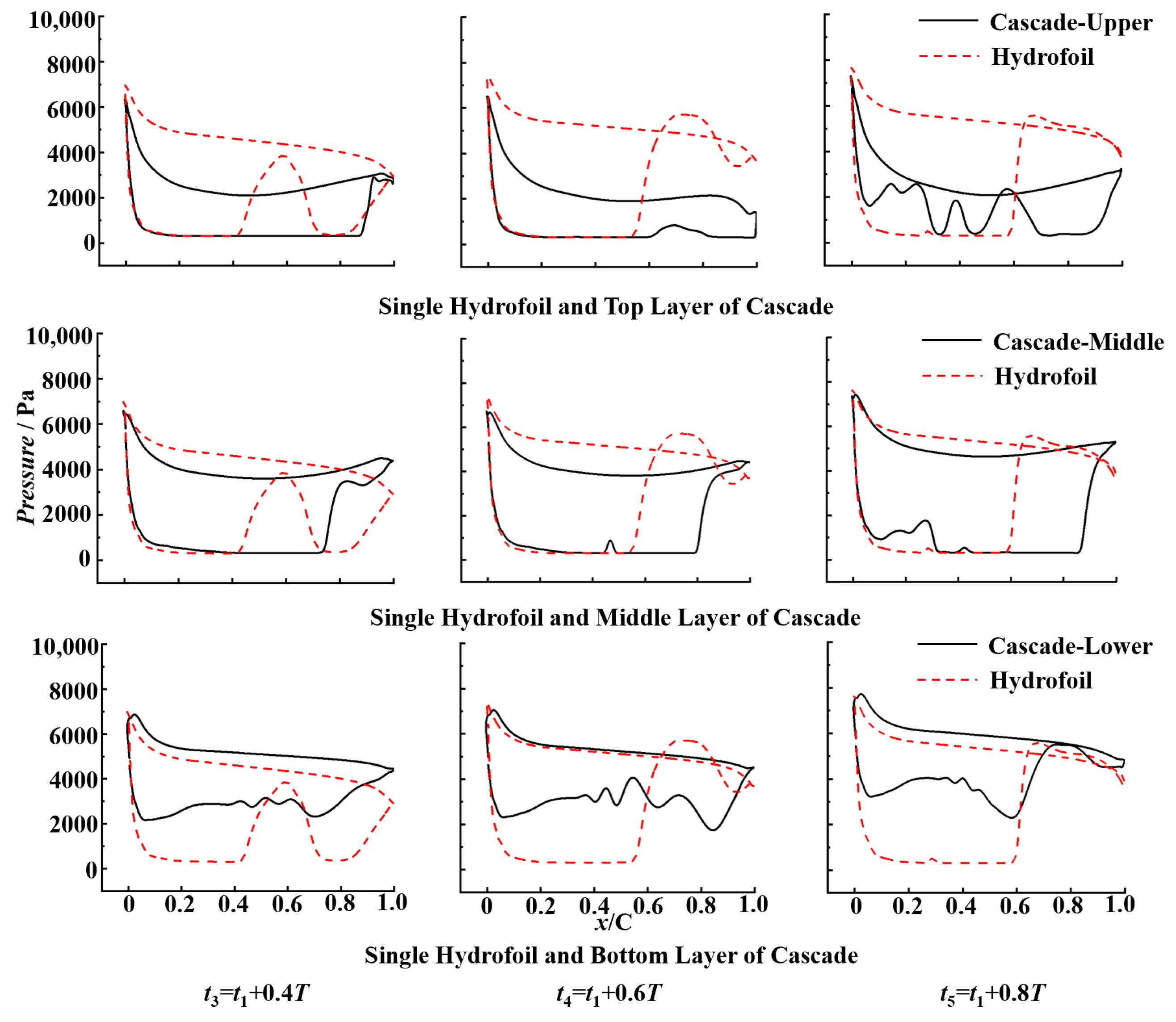
Figure 16 displays the pressure distribution in the x-direction for the single hydrofoil and the cascade at three distinct time instants. The lower curves represent the pressure on the suction side (low-pressure regions), while the upper curves represent the pressure on the pressure side (high-pressure regions). The area enclosed by the upper and lower curves represents the lift experienced by the hydrofoil at that specific cross-section. Comparing the plots, it is evident that, at t = t 3 , the suction side of the top hydrofoil in the cascade is entirely in a low-pressure state, approaching the saturated vapor pressure. In contrast, the cavitation intensity on the single hydrofoil is weaker, with the cavity failing to fully cover the surface, resulting in a high-pressure region at the trailing edge. Because the pressure-side pressure of the single hydrofoil is significantly higher than that of the top hydrofoil, the lift characteristics of the single hydrofoil are more prominent at this instant. At t = t 4 , a comparison of the pressure distributions between the single hydrofoil and middle hydrofoil reveals that, since no significant attached cavity appears on the bottom hydrofoil, the suction-side pressure of the middle hydrofoil is markedly higher than that of the top layer. Particularly at t = t 5 , the lift provided by the middle hydrofoil surpasses that of the top hydrofoil. Furthermore, because the pressure side of the bottom hydrofoil is unaffected by the cascade structure, its pressure remains consistent with that of the single hydrofoil; however, due to the absence of surface cavitation, the pressure difference between the upper and lower surfaces is not pronounced, thus failing to enhance the overall lift of the cascade.
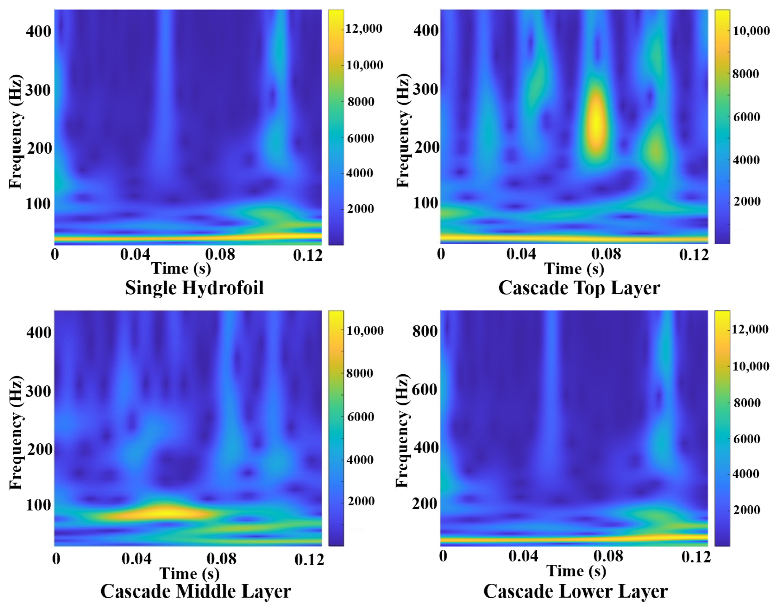
The surface pressures of the single hydrofoil and cascade exhibit periodic fluctuations corresponding to the shedding and collapse of cavities. Figure 17 presents the time–frequency analysis results of the lift at the monitoring points located at the center of the single hydrofoil and cascade layers, obtained through a Continuous Wavelet Transform (CWT). It can be observed that the cavity collapse frequency for the single hydrofoil remains stable at approximately 40 Hz, while the collapse frequency for the top hydrofoil of the cascade is similar, at 45 Hz. Furthermore, the figure clearly demonstrates transient and intense fluctuations in the lift of the top hydrofoil, reaching a frequency of 250 Hz, which corresponds to the transient shock waves and pressure pulses generated by the violent collapse of large-scale detached cavities. The intensity of these high-frequency fluctuations in the top layer confirms the presence of more aggressive cavity implosions compared to the lower layers, where large-scale cavitation is suppressed. Meanwhile, the cavity collapse frequency on the middle hydrofoil increases to approximately 70 Hz due to the influence of the cascade structure, with the lift exhibiting similar fluctuations. In contrast, no large-scale cavities are generated on the surface of the bottom hydrofoil, and its lift fluctuation frequency remains basically stable at 50 Hz.

4. Conclusions

Based on experimental and numerical investigations of unsteady cavitating flows around a single hydrofoil and cascade, this study systematically analyzes the evolutionary processes and dynamic characteristics of cavitation at different cascade positions. The key findings are summarized as follows:
  • The cascade’s internal structure significantly modulates cavitation inception and development. At the inception and sheet cavitation stages, the suction-side interaction of the top hydrofoil creates a more uniform pressure field, thereby inhibiting and delaying cavitation in the middle and bottom layers. During the cloud cavitation stage, the top layer mirrors the behavior of an isolated hydrofoil, characterized by large-scale shedding. Conversely, the middle and bottom layers exhibit shortened cavitation cycles with less pronounced re-entrant jets and shedding scales. This characteristic helps mitigate cavitation erosion damage caused by the periodic collapse of cavities. At the super-cavitation stage, the middle layer transitions more rapidly due to downstream cavity development.
  • The cascade structure limits the formation of large-scale shedding in internal layers, favoring chord-wise cavity extension instead. This study identifies that both re-entrant jet and shock wave mechanisms drive cavity collapse in the cloud stage. While the top layer exhibits distinct re-entrant jet and shock wave phenomena, the shock wave mechanism is significantly attenuated in the middle and bottom layers due to the modified internal flow environment. In the design process, asymmetric optimization should be performed for the hydrofoils at different positions.
  • Hydrodynamic forces on the cascade scale approximately threefold relative to a single hydrofoil, reflecting the cumulative effect of the three-foil configuration. However, the top-layer hydrofoil experiences restricted lift and disproportionately higher drag compared to the internal layers. This suggests that optimizing the leading-edge or surface profile of the top hydrofoil is a critical pathway for enhancing the overall hydrodynamic efficiency of the cascade.
  • The lift on the top hydrofoil’s suction side is suppressed by the internal low-pressure field of the cascade, leading to a lower lift coefficient than that of an isolated foil. The middle hydrofoil exhibits complex lift fluctuations due to the dual influence on its suction and pressure sides, while the bottom layer remains stable with minimal cavitation. The cavity collapse frequencies for the top, middle, and bottom hydrofoils within the cascade are 45 Hz, 70 Hz, and 50 Hz, respectively, which closely align with the dominant frequencies of their respective lift fluctuations. In practical engineering, the natural frequency of the structure should be adjusted according to the dominant frequency characteristics to avoid fluid–structure resonance under specific cavitation numbers.

Author Contributions

Conceptualization, W.B. and F.C.; methodology, W.B.; software, W.B. and Y.Z.; validation, W.B. and Y.D.; formal analysis, W.B. and Y.Z.; investigation, M.Z.; resources, W.B.; data curation, Y.Z.; writing—original draft preparation, W.B.; writing—review and editing, W.B., Y.Z. and F.C.; visualization, W.B.; supervision, M.Z. All authors have read and agreed to the published version of the manuscript.

Funding

This work was supported by the Integration Program of the National Natural Science Foundation of China (Grant No. U22B6010).

Data Availability Statement

The original contributions presented in this study are included in the article. Further inquiries can be directed to the corresponding author.

Conflicts of Interest

The authors declare no conflict of interest.

References

  1. Zhang, X.M. Optimal launch capacity trajectory design for SpaceX’s super heavy starship launch vehicle. Proc. SPIE 2023, 12921, 1039–1042. [Google Scholar]
  2. Yang, Y.; Huang, L.L.; Kuznetsov, N.V.; Lai, Q. Design and Implementation of Grid-Wing Hidden Chaotic Attractors with Only Stable Equilibria. IEEE Trans. Circuits Syst. Regul. Pap. 2023, 11, 6492–6503. [Google Scholar] [CrossRef] [Scilit]
  3. Iga, Y.; Yoshida, Y. Numerical Analysis of Controlling Cavitation Instabilities in Tandem Cascades. Trans. Jpn. Soc. Aeronaut. Space Sci. 2011, 54, 137–143. [Google Scholar] [CrossRef] [Scilit]
  4. Lin, S.C.; Yan, J.; Pan, X.; Liu, J.F.; Wang, X. Analysis Method of Unfolding Dynamic Characteristics of Non-damping Rod Type Grid Fins. Missiles Space Veh. 2018, 5, 16–20. [Google Scholar] [CrossRef]
  5. Ji, B.; Bai, X.; Zhu, Y.; Cheng, H.; Peng, X.; Long, X. A review of the fundamental investigations of cavitation in hydraulic machinery. Chin. J. Hydrodyn. 2017, 32, 542–550. [Google Scholar]
  6. Li, W.X.; Li, Z.G.; Qin, Z.; Yan, S.; Wang, Z.; Peng, S. Influence of the solution pH on the design of a hydro-mechanical magneto hydraulic sealing device. Eng. Fail. Anal. 2022, 135, 106091. [Google Scholar]
  7. Sun, H. Numerical study of hydrofoil geometry effect on cavitating flow. J. Mech. Sci. Technol. 2012, 26, 2535–2545. [Google Scholar] [CrossRef] [Scilit]
  8. Truscott, T.T.; Epps, B.P.; Belden, J. Water Entry of Projectiles. Annu. Rev. Fluid Mech. 2014, 46, 355–378. [Google Scholar] [CrossRef] [Scilit]
  9. Thoroddsen, S.T.; Etoh, T.G.; Takehara, K.; Takano, Y. Impact jetting by a solid sphere. J. Fluid Mech. 2004, 499, 139–148. [Google Scholar] [CrossRef] [Scilit]
  10. Tian, B.C.; Li, L.M.; Huang, B. Investigation into the Multiscale Characteristics of Cavitation Flow under Different Cavity Shedding Mechanism. Chin. J. Hydrodyn. 2024, 39, 87–96. [Google Scholar]
  11. Peng, K.; Hu, F.; Zhang, W.; Zhou, Z. Review of aerodynamic characteristics and application of grid fin. Guti Huojian Jishu/J. Solid Rocket. Technol. 2015, 38, 458–464. [Google Scholar]
  12. Ji, B.; Cheng, H.Y.; Huang, B.; Luo, X.; Peng, X.; Long, X. Research progresses and prospects of unsteady hydrodynamics characteristics for cavitation. Adv. Mech. 2019, 49, 428–479. [Google Scholar]
  13. Wang, Z.; Cheng, H.Y.; Ji, B. Euler-Lagrange study of cavitating turbulent flow around a hydrofoil. Phys. Fluids 2021, 33, 112108. [Google Scholar] [CrossRef] [Scilit]
  14. Qu, S.; Li, J.; Cheng, H.; Ji, B. LES investigation on vortex dynamics of transient sheet/cloud cavitating flow using different vortex identification methods. Mod. Phys. Lett. B 2020, 34, 2150011. [Google Scholar] [CrossRef] [Scilit]
  15. Movahedian, A.; Pasandidehfard, M.; Roohi, E. LES investigation of sheet-cloud cavitation around a 3-D twisted wing with a NACA 16012 hydrofoil. Ocean. Eng. 2019, 192, 106547. [Google Scholar] [CrossRef] [Scilit]
  16. Su, T.C.; Zhang, J.; Cai, X.W. Research on Hydrodynamic Characteristics of Grid Wall Profile. In Proceedings of the Chinese Congress of Theoretical and Applied Mechanics (CCTAM 2019), Hangzhou, China, 25–28 August 2019; Chinese Society of Theoretical and Applied Mechanics: Beijing, China, 2019. [Google Scholar]
  17. Ma, P.; Wang, Y.; Xie, Y.; Han, J.; Sun, G.; Zhang, J. Effect of wake interaction on the response of two tandem oscillating hydrofoils. Energy Sci. Eng. 2019, 7, 431–442. [Google Scholar] [CrossRef] [Scilit]
  18. Raj, K.M.; Arumuru, V. Jet deflection by two side-by-side arranged hydrofoils pitching in a quiescent fluid. AIP Adv. 2020, 10, 105128. [Google Scholar] [CrossRef] [Scilit]
  19. Yu, A.; Feng, W.J.; Tang, Q.H. Large Eddy Simulation of the cavitating flow around a Clark-Y mini cascade with an insight on the cavitation-vortex interaction. Ocean. Eng. 2022, 266, 112852. [Google Scholar] [CrossRef] [Scilit]
  20. Xu, M.H.; Cheng, H.Y.; Ji, B.; Peng, X. Prediction method of tip vortex circulation based on hydrofoil load. Ocean. Eng. 2023, 288, 116176. [Google Scholar] [CrossRef] [Scilit]
  21. Zhao, G.S.; Liu, H.; Wu, R.; Liang, N.; Cao, L. Statistical study of cascade hydrodynamics and cavitation dynamics in propulsion pumps. Int. J. Nav. Archit. Ocean. Eng. 2025, 17, 100665. [Google Scholar] [CrossRef] [Scilit]
  22. Ye, K.; Zhang, Y.F.; Chen, Z.S.; Ye, Z. Numerical Investigation of Aeroelastic Characteristics of Grid Fin. AIAA J. 2021, 60, 3107–3121. [Google Scholar] [CrossRef] [Scilit]
  23. Zhu, Y.H.; Zhou, Z.H.; Li, Y.; Shen, L.; Jiang, Y. Design and Underwater Numerical Analysis of Grid Fins Based on Negative Pressure Gradient Foils. J. Ballist. 2023, 35, 52–59. [Google Scholar]
  24. Ondřej, B.; Václav, H.; Jan, V. Convolution neural network for fluid flow simulations in cascade with oscillating blades. J. Comput. Appl. Math. 2025, 462, 116478. [Google Scholar] [CrossRef] [Scilit]
  25. Delale, C.F.; Nas, S.; Tryggvason, G. Direct numerical simulations of shock propagation in bubbly liquids. Phys. Fluids 2005, 17, 121705. [Google Scholar] [CrossRef] [Scilit]
  26. Coutier-Delgosha, O.; Fortes-Patella, R.; Reboud, J.L. Evaluation of the Turbulence Model Influence on the Numerical Simulations of Unsteady Cavitation. J. Fluids Eng. 2003, 125, 38–45. [Google Scholar] [CrossRef] [Scilit]
  27. Huang, B.; Zhao, Y.; Wang, G. Large Eddy Simulation of turbulent vortex-cavitation interactions in transient sheet/cloud cavitating flows. Comput. Fluids 2014, 92, 113–124. [Google Scholar] [CrossRef] [Scilit]
  28. Roohi, E.; Zahiri, A.P.; Passandideh-Fard, M. Numerical simulation of cavitation around a two-dimensional hydrofoil using VOF method and LES turbulence model. Appl. Math. Model. 2013, 37, 6469–6488. [Google Scholar] [CrossRef] [Scilit]
  29. Wosnik, M.; Arndt, R.E.A. Identification of Large Scale Structures in Cavitating Wakes. In Fluids Engineering Division Summer Meeting; ASME: New York, NY, USA, 2007; pp. 1473–1474. [Google Scholar]
  30. Bensow, R.E.; Bark, G. Implicit LES Predictions of the Cavitating Flow on a Propeller. J. Fluids Eng. 2010, 132, 041302. [Google Scholar] [CrossRef] [Scilit]
  31. Zwart, P.J.; Gerber, A.G.; Belamri, T. A two-phase flow model for predicting cavitation dynamics. In Proceedings of the 5th International Conference on Multiphase Flow, Yokohama, Japan, 30 May–4 June 2004. [Google Scholar]
  32. ANSYS. ANSYS ICEM CFD User’s Guide; ANSYS, Inc.: Canonsburg, PA, USA, 2023. [Google Scholar]
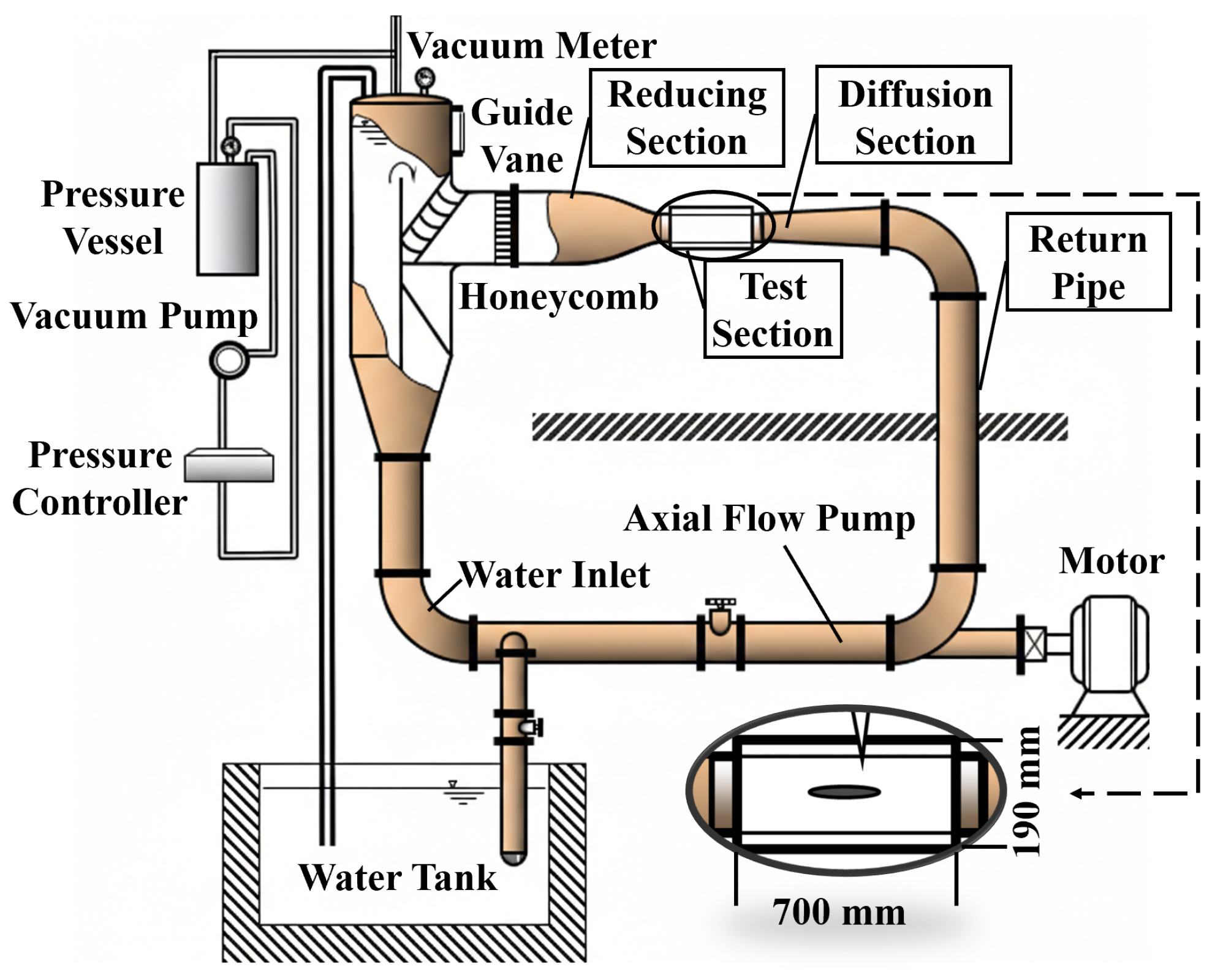
Figure 1. Schematic of cavitation water tunnel.
Jmse 14 00620 g001
Figure 2. Fabricated cascade model.
Jmse 14 00620 g002
Figure 3. Schematic of the PIV velocity field measurement system.
Jmse 14 00620 g003
Figure 4. Cascade computational domain.
Jmse 14 00620 g004
Figure 5. Mesh generation of the cascade.
Jmse 14 00620 g005
Figure 6. Comparison between experimental (top) and numerical (bottom) results for single hydrofoil/cascade.
Jmse 14 00620 g006
Figure 7. Comparison between numerical velocity vectors (left) and PIV velocity field measurements (right) for the cascade.
Jmse 14 00620 g007
Figure 8. Cavity patterns of the single hydrofoil and the cascade at different cavitation stages.
Jmse 14 00620 g008
Figure 9. Evolution of maximum relative cavity length with cavitation number for the single hydrofoil and different positions within the cascade.
Jmse 14 00620 g009
Figure 10. Pressure contours, velocity contours, and streamlines for the single hydrofoil and cascade.
Jmse 14 00620 g010
Figure 11. Schematic of cavity structures during cavitation inception in the cascade.
Jmse 14 00620 g011
Figure 12. Cavity patterns of the cascade during the cloud cavitation stage.
Jmse 14 00620 g012
Figure 13. Variation in cavitation bubble shedding frequency ( f s h e d ) and Strouhal number ( S t L ) with cavitation number for different positions of single hydrofoil and cascade.
Jmse 14 00620 g013
Figure 14. Dynamic characteristics versus cavitation number ( σ ) for the single hydrofoil and cascade. (a) Lift coefficient ( C L ) versus cavitation number ( σ ) for single hydrofoil and cascade; (b) Drag coefficient ( C d ) versus cavitation number ( σ ) for the single hydrofoil and the cascade.
Jmse 14 00620 g014
Figure 15. Time evolution of lift and drag coefficients ( C L and C d ) for the single hydrofoil and cascade at σ = 1.24 .
Jmse 14 00620 g015
Figure 16. Pressure distributions along the x-direction for the single hydrofoil and different positions within the cascade at σ = 1.24 .
Jmse 14 00620 g016
Figure 17. Time–frequency analysis of lift coefficient ( C L ) for the single hydrofoil and cascade at σ = 1.24 .
Jmse 14 00620 g017
Table 1. Verification of grid independence.
Number of Grids ( × 10 4 ) C L C d
1871.077975890.0904817
2901.045018990.0780917
3651.043868620.0943425
4761.043441520.0819988
5821.043581350.0812062
Table 2. Verification of time-step independence.
Time Step (s) C L C d
1 × 10 3 2.152844300.3350498
5 × 10 4 1.742958370.2597309
1 × 10 4 1.184720460.1082533
5 × 10 5 1.043441520.0819988
1 × 10 5 1.043523720.0817264
Table 3. Relative error between experimental and numerical results for the single hydrofoil and the cascade.
E r e l 2.001.881.731.411.080.60
Relative error of the cavity area for the single hydrofoil3.53%2.36%3.08%2.14%1.85%2.04%
E r e l 1.581.761.451.240.840.64
Relative error of the cavity area for the cascade4.28%3.55%3.72%3.10%3.37%3.19%
Disclaimer/Publisher’s Note: The statements, opinions and data contained in all publications are solely those of the individual author(s) and contributor(s) and not of MDPI and/or the editor(s). MDPI and/or the editor(s) disclaim responsibility for any injury to people or property resulting from any ideas, methods, instructions or products referred to in the content.