IMU-Enhanced Vessel Trajectory Prediction: Overcoming Kinematic Lag and Distribution Shift in Sparse Data Engineering Scenarios

Abstract

Vessel trajectory prediction is pivotal for maritime traffic safety and autonomous collision avoidance. However, existing studies predominantly rely on massive public AIS (Automatic Identification System) datasets, often overlooking the challenges of data sparsity and long-tailed distributions inherent in practical engineering scenarios, where high-dynamic maneuvering samples are scarce. Furthermore, as a low-frequency kinematic observation system, AIS suffers from inherent kinematic lag relative to the vessel’s true dynamic state, particularly failing to timely reflect turning intentions during the maneuver initiation phase. To address these challenges, this paper proposes a Physics-Aware Multimodal Fusion Framework. By incorporating high-frequency acceleration and angular velocity from an Inertial Measurement Unit (IMU), the framework applies physical compensation to AIS kinematic observations, thereby enhancing the model’s perception of maneuvering intent. Validation based on real-vessel experimental data demonstrates that the proposed method effectively mitigates the prediction lag observed in pure-AIS models at the 60 s horizon, significantly improving accuracy in turning scenarios. Moreover, in 180 s long-term predictions, the multimodal fusion mechanism effectively suppresses integration drift, ensuring superior trajectory shape consistency and engineering stability. The study indicates that incorporating IMU inertial information is critical for enhancing the robustness of vessel trajectory prediction under practical engineering conditions characterized by sparse samples and complex maneuvers.

1. Introduction

As global economic integration deepens, maritime trade has become the nexus of the world economy, handling over 80% of international trade transportation. Recently, with the International Maritime Organization (IMO) advancing regulations for Maritime Autonomous Surface Ships (MASS), the digitalization and intelligent transformation of the shipping industry have accelerated [1]. In intelligent navigation scenarios, accurate spatiotemporal positioning is a prerequisite for safety. Vessels typically rely on the Global Navigation Satellite System (GNSS) as their primary source [2]. However, satellite signals are prone to interruption, drift, or denial in complex sea states or port environments, compromising the continuity and reliability of positioning [3,4]. Maintaining situational awareness through effective modeling of vessel motion during GNSS anomalies has thus become a critical safety issue. Trajectory prediction serves as a foundational technology bridging historical observations with future motion states, supporting autonomous collision avoidance and intelligent decision-making.

The Automatic Identification System (AIS), a standardized global maritime monitoring technology, provides spatiotemporal data such as position, speed, and course [5]. Although it relies on onboard GNSS, it offers rich high-dimensional data for maritime research. By analyzing historical and current AIS data, researchers have developed various trajectory prediction models, achieving significant success on public datasets and supporting Vessel Traffic Services (VTS) [6,7,8]. Beyond directly safeguarding navigational safety, high-precision, maneuverability-aware trajectory prediction can also serve as foundational data input for broader maritime operational analyses. Consequently, it is capable of supporting various downstream maritime decision-making processes, such as berth congestion mitigation and demurrage pattern analysis [9]. However, modeling based solely on historical AIS trajectories struggles to cover all maneuvering encountered situations in actual navigation. Specifically, under high-dynamic conditions—such as emergency avoidance, sharp turning, or rapid speed changes—relevant motion patterns are often scarce or under-observed in historical data, rendering models ineffective for such states. Moreover, existing studies are largely trained on idealized, massive public datasets, which differ significantly from practical engineering scenarios. In real-world maritime intelligent traffic systems, models universally face small sample sizes and long-tailed distributions: newly launched or mission-specific vessels lack long-term data accumulation, and the vast majority of samples correspond to steady-state straight sailing, while high-dynamic maneuvering samples are extremely rare. Deep learning models trained on such imbalanced data tend to overfit to straight-line modes, failing to capture instantaneous motion changes. This leads to severe prediction lag or divergence during the maneuver initiation phase. Therefore, an effective approach is required to enhance the model’s maneuver perception capability without compromising its ability to learn from historical features.

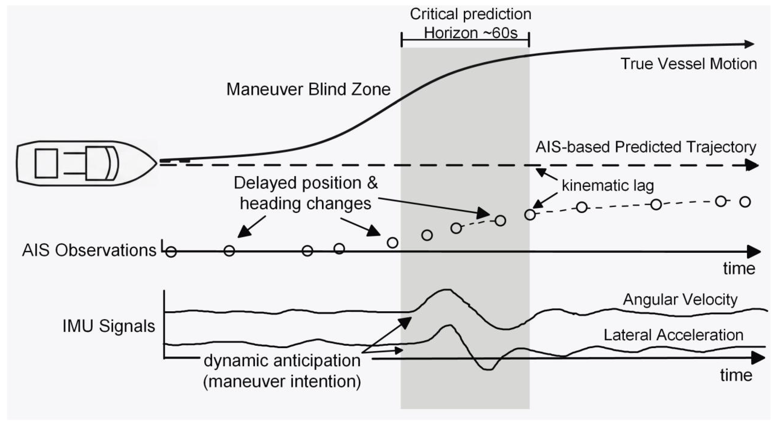
Existing models relying solely on AIS data are insufficient for practical engineering needs. To address performance degradation caused by AIS observation lag and the scarcity of complex maneuvering samples, this paper introduces the Inertial Measurement Unit (IMU) as a physical supplement. The IMU provides high-frequency attitude vessel (roll, pitch, heading) and acceleration data. Physically, changes in attitude and acceleration precede changes in position, meaning IMU data contains prior dynamic information reflecting maneuvering intention. Based on this, we propose a vessel trajectory prediction method based on IMU enhancement, which utilizes synchronized AIS and IMU raw data collected from real vessel experiments to construct a multimodal deep learning model. While retaining the modeling advantages of historical AIS trajectory features, this model further enhances the model’s perception ability and trajectory prediction accuracy for high-dynamic maneuvering behavior.

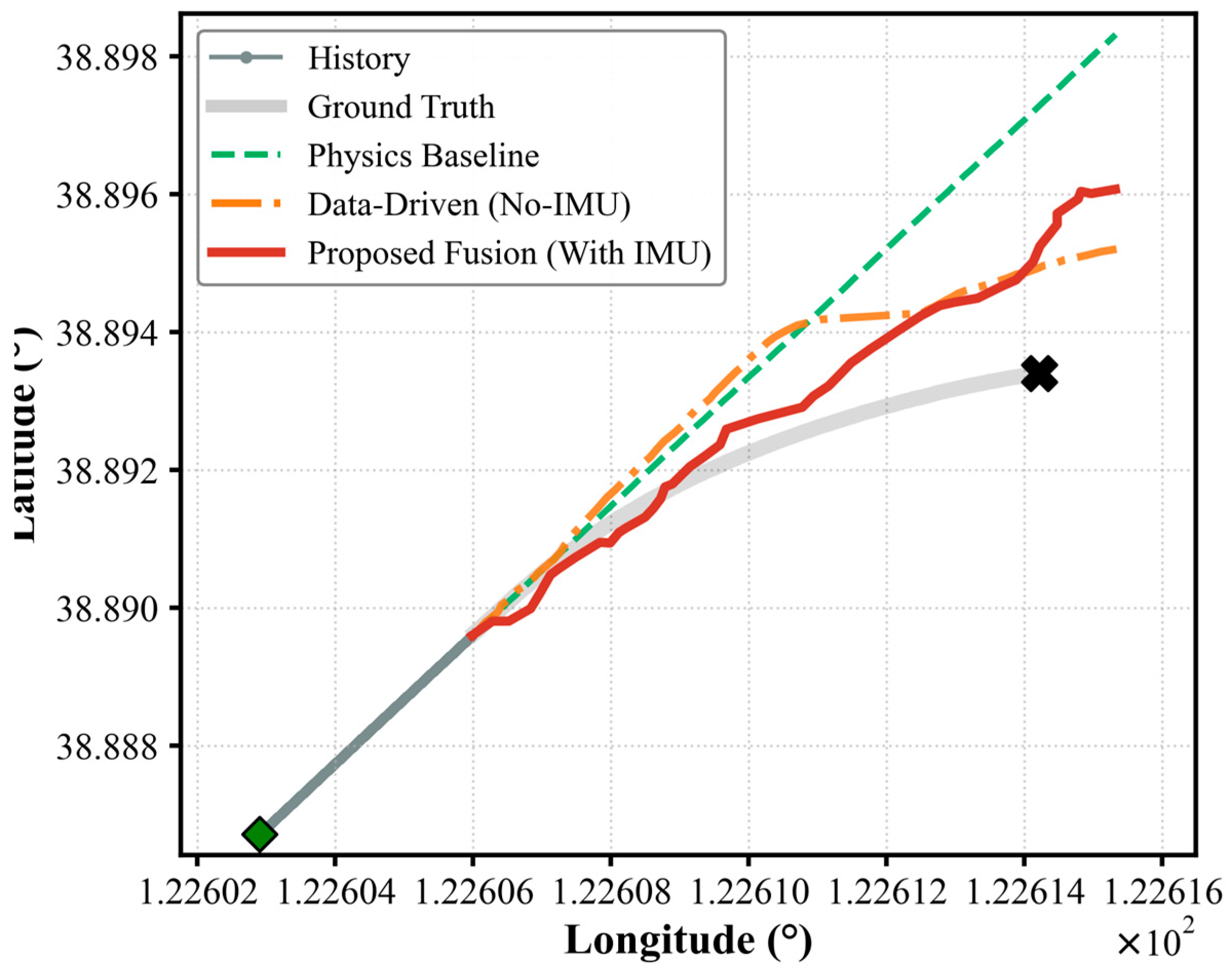
This paper focuses on the physical observability constraint in practical engineering. During the transition from steady sailing to maneuvering (e.g., turning), AIS-derived kinematic information (position, speed, course) inherently lags behind the vessel’s true dynamic state. Given the large inertia of vessels and limited sensor sampling rates, relying solely on AIS leads to insufficient perception during the maneuver initiation phase, affecting prediction stability. Unlike studies pursuing marginal accuracy improvements on idealized datasets, this research systematically analyzes the physical boundaries of trajectory prediction under engineering constraints (small samples, long-tailed distributions, limited sensors) and explores a feasible breakthrough. We prioritize stability, physical consistency, and safety availability in engineering applications, in order to provide practical technical support for the safe navigation of intelligent vessels. Building upon the clarification of the aforementioned engineering objectives, it is necessary to further elucidate the fundamental methodological distinctions between the proposed framework and existing approaches. Compared to classical sensor fusion techniques widely adopted in the robotics domain (e.g., the Extended Kalman Filter, EKF)—which fundamentally focus on short-term state estimation and smoothing under the Markov assumption—our framework targets long-horizon trajectory prediction (up to 180 s). EKF-based methods struggle to extrapolate complex, non-linear, and human-driven maneuvering intentions over extended time scales. Within our framework, Inertial Measurement Unit (IMU) data is not utilized merely for instantaneous state filtering. Instead, it serves as a high-frequency dynamic trigger, empowering the deep learning attention mechanism to proactively anticipate macroscopic trajectory shifts before low-frequency AIS records any significant spatial displacement. Furthermore, compared to recent deep learning-based maritime trajectory prediction models, our approach introduces a physics-aware paradigm. Due to the inherent “kinematic lag” of AIS and the long-tailed distribution of maritime maneuvers, traditional deep models suffer severe performance degradation in sparse data scenarios. Our framework structurally compensates for this deficiency by directly embedding physical kinematic constraints (IMU dynamic priors) and a maneuver-aware dynamic loss function, thereby transforming the model from a “passive data fitter” into a “proactive, physics-informed predictor. The main contributions of this study are as follows:

Construction of a Physics-Aware Multimodal Fusion Framework: We propose a deep learning model fusing AIS position data with IMU attitude features. By integrating attitude dynamics, we compensate for the limitations of kinematic-only AIS data, significantly enhancing prediction accuracy in complex maneuvering scenarios.

Benchmark comparison and model evaluation: To comprehensively evaluate the contribution of IMU features to prediction performance, we selected the Transformer attention model and the LSTM recurrent model, and conducted experimental comparative analysis before and after integrating IMU features into both models.

Effectiveness verification in practical engineering: By constructing a deep learning model using synchronous AIS and IMU raw data collected from real vessel experiments, it is proven that in practical engineering scenarios with small samples and long-tailed distributions, the introduction of inertial information is crucial for overcoming the physical limits of a single modality and achieving robust trajectory prediction.

This study unfolds as follows: Section 2 reviews relevant work on vessel trajectory prediction, Section 3 proposes a physical perception multimodal fusion method, detailing data preprocessing, model structure, loss function, and engineering constraints, Section 4 describes the real-vessel experimental platform, dataset, and comparison setup, Section 5 verifies the effectiveness of the method through multi-scenario experiments and ablation analysis, and Section 6 summarizes the full paper and outlines future research directions.

2. Related Work

Vessel trajectory prediction has consistently been a research hotspot in the fields of intelligent navigation and ocean engineering [10,11,12]. Depending on the modeling mechanisms and input data, existing prediction methods can be broadly categorized into two main classes: physics-based kinematic methods and data-driven methods. Furthermore, multi-source data fusion methods, which have emerged in recent years, are gradually becoming a new trend in research.

Regarding physics-based kinematic methods, early vessel trajectory prediction primarily relied on vessel hydrodynamic equations and state estimation techniques. These approaches focused on intrinsic driving factors, utilizing only the target vessel’s historical motion patterns for prediction [13,14,15,16]. The Kalman Filter (KF) and its variants—such as the Extended Kalman Filter (EKF) and Unscented Kalman Filter (UKF)—are the most classical methods in this domain. Perera et al. [17] implemented real-time trajectory estimation by combining EKF with a vessel maneuvering motion model. Laxhammar [18] employed unsupervised clustering methods to predict vessel traffic patterns, utilizing Gaussian Mixture Models (GMM) as the clustering model and the Expectation-Maximization (EM) algorithm. These methods possess the advantages of computational efficiency and strong physical interpretability. However, physical models are typically established on assumptions of idealized force states or linear motion and rely heavily on precise hydrodynamic coefficients. In actual sea conditions, when facing strong non-linear disturbances from wind, waves, and currents, or when vessels undergo complex maneuvers, the long-term prediction accuracy of such methods is often difficult to guarantee due to the challenges in establishing precise mathematical model parameters in real-time, rendering them prone to cumulative errors.

Regarding data-driven methods, with the proliferation of AIS data and the enhancement of computational power, these approaches have gradually assumed a dominant role, primarily comprising traditional machine learning and deep learning methods. In the realm of traditional machine learning, methods such as Support Vector Regression (SVR) and Gaussian Process Regression (GPR) have been widely applied to trajectory regression tasks. Liu et al. [19] utilized an improved SVR model to enhance trajectory prediction accuracy. Although these methods perform acceptably with small sample sizes, their feature extraction capabilities and generalization often prove insufficient when processing massive, high-dimensional AIS data characterized by temporal dependencies. In contrast, deep learning methods have demonstrated superior advantages. Recurrent Neural Networks (RNN) and their variants—Long Short-Term Memory (LSTM) and Gated Recurrent Unit (GRU)—have become the mainstream choices for trajectory prediction due to their unique gating mechanisms, which effectively handle long-term dependencies in time-series data. Chen et al. [20] proposed a deep learning model for curve fitting and analysis based on AIS data. This method consists of a forward GRU and a backward Bi-directional GRU (Bi-GRU) network, thereby reducing the scope of the trajectory to be fitted by scaling in both directions. Zhang et al. [21] proposed a trajectory prediction method combining AIS information with LSTM networks, achieving real-time prediction of future vessel trajectories. Billah et al. [22] introduced a prediction model based on an encoder–decoder architecture, which encodes past temporal AIS data to generate future trajectory samples. Recently, following the success of attention mechanisms in Natural Language Processing (NLP), Transformer-based architectures have also been introduced to trajectory prediction. Transformers can parallelly capture global dependencies within sequences through self-attention mechanisms. Xue et al. [23] proposed the G-Trans model based on the Transformer architecture, further improving prediction accuracy and demonstrating the potential of advanced deep learning architectures in mining spatiotemporal trajectory features.

Despite the excellent performance of the aforementioned methods on large-scale public datasets, they often falter when addressing small sample problems in practical engineering contexts. Most studies rely on training with massive historical data, overlooking the issue of data sparsity for specific vessels in real-world applications. Particularly when confronting long-tailed distribution characteristics, existing models tend to minimize average error by memorizing high-frequency straight-sailing patterns. Consequently, when rare maneuvering behaviors (such as large-angle turns) occur in testing scenarios, models suffer from distribution shift due to the lack of sufficient feature mapping samples, leading to trajectory divergence. This indicates that end-to-end learning relying solely on AIS data exhibits a significant robustness bottleneck in scenarios lacking the support of massive datasets.

While existing deep learning models have enhanced prediction performance, relying solely on AIS data (position, speed, course) presents inherent limitations. AIS data is characterized by low update frequencies (typically ranging from seconds to minutes) and is highly susceptible to signal packet loss and noise interference. To mitigate this issue, some scholars have explored multi-source data fusion to construct vessel trajectory prediction models. For instance, Murray and Huang et al. [24,25] incorporated external factors such as meteorological and hydrological conditions, as well as interactive trajectories of neighboring vessels, to enrich input features for auxiliary prediction. Zhang et al. [26] attempted to introduce environmental data (wind, waves, currents) to correct prediction results, aiming to improve accuracy through environmental constraints within the model. Lin et al. [27] utilized visual imagery and radar data to enhance perception of the surrounding environment and assist in determining vessel position. However, the aforementioned multi-source fusion methods predominantly focus on traffic flow prediction in macro-scale waters or rely heavily on interactive information from neighboring vessels. In practical navigation, the primary concern for a vessel is the safety of its own motion state. Particularly in extreme areas where satellite signals are subject to interference, not only may the own vessel’s high-precision positioning signals be lost, but obtaining position information of surrounding vessels also faces significant difficulties [28,29]. This exposes prediction models relying on global spatiotemporal dependencies or neighbor interactions to the risk of failure in practical applications. Therefore, research on independent trajectory prediction focused on the local scale of the own vessel, decoupled from excessive reliance on external environmental information, holds significant engineering significance [30].

Furthermore, research addressing the impact of vessel body attitude—specifically roll, pitch, and high-frequency acceleration—on trajectory prediction remains relatively scarce. In the fields of autonomous driving and robotics, the Inertial Measurement Unit (IMU) has been proven to significantly enhance the robustness of localization and prediction, especially when GPS signals are limited or vehicles undergo highly dynamic maneuvers [31,32,33]. In the maritime domain, IMU data is typically restricted to stability monitoring, and its application value in trajectory prediction has not yet been fully exploited. Crucially, the high-frequency dynamic features provided by the IMU can physically compensate for the kinematic lag of AIS data, providing the model with more direct perception of maneuvering intentions. Consequently, we propose a multi-source data fusion model integrating AIS and IMU data to enhance vessel trajectory prediction capabilities.

In summary, existing studies have predominantly concentrated on improving deep learning network structures or fusing external environmental information to boost trajectory prediction performance, while largely overlooking the dynamic trend information embedded in the vessel’s own high-frequency attitude data—information that can often anticipate vessel maneuvering intentions. To address this problem, this paper constructs a vessel trajectory prediction framework tailored for engineering scenarios characterized by small samples and long-tailed distributions, by fusing high-frequency IMU data with AIS data. This approach aims to enhance the prediction stability and reliability of the model under complex maneuvering conditions.

3. Methodology

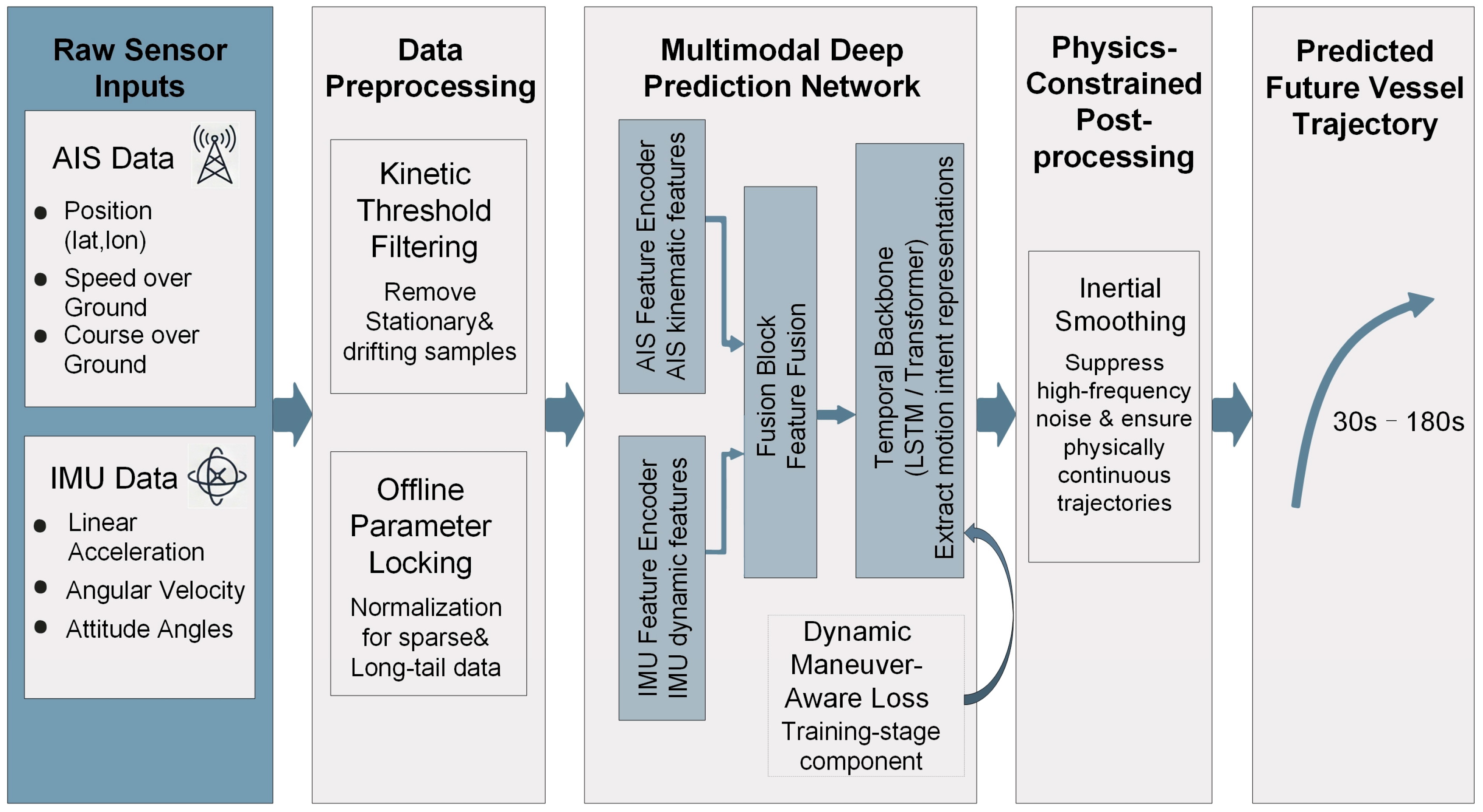
To address the challenges of long-tailed distributions and small-sample constraints prevalent in practical engineering scenarios, a Physics-Aware Multimodal Fusion Framework is proposed. This framework comprises three integral components: data preprocessing, a multimodal deep prediction network, and engineering-constrained post-processing. AIS data primarily provides kinematic observations based on position and speed, which inevitably suffer from kinematic lag during the maneuver initiation phase. In contrast, the angular velocity and linear acceleration collected by the IMU more directly reflect variations in the vessel’s attitude and force states. Leveraging these complementary characteristics, a multimodal feature fusion mechanism is incorporated into the model design. This mechanism enhances the perception of maneuvering intention, laying a foundation for improving trajectory prediction robustness during both the initial maneuvering stage and over long prediction horizons. The overall fusion framework is illustrated in Figure 1. It consists of three main components: a data preprocessing module, a multimodal deep prediction network, and an engineering-constrained post-processing module.

Data Preprocessing Module: To address the issues of noise interference and mixed operating conditions inherent in raw AIS and IMU data collected from real-world trials, preprocessing subject to physical consistency constraints is first applied to the sensor data. Considering that vessels in anchoring or ultra-low speed drifting states exhibit a high ratio of random noise in their AIS position and attitude information, and that such data lacks distinct maneuvering behavioral features in a dynamic sense, direct utilization for model training would likely interfere with the learning of valid navigation states. Therefore, a kinetic energy threshold filtering mechanism based on vessel speed is constructed. Trajectory segments below a preset speed threshold are excluded, effectively removing low-information samples such as anchoring and low-speed drifting, ensuring that the training data primarily covers navigation conditions with definitive motion significance. Furthermore, under conditions of small samples and long-tailed distributions, relying directly on training data statistics for normalization can easily lead to feature scale instability due to fluctuations in sample composition. To mitigate this, an offline parameter locking strategy is introduced. By incorporating statistical features from typical vessel navigation states, normalization parameters are pre-fixed. This prevents the introduction of additional bias caused by data distribution shifts between training and inference phases, providing stable data input conditions for subsequent model learning.

Multimodal Deep Prediction Network: upon completion of data preprocessing, we construct a multimodal deep learning prediction model fusing AIS and IMU information to model and predict future vessel trajectories. This model is primarily composed of three key sub-modules: modal feature encoding, feature fusion, and temporal modeling. First, AIS kinematic features and IMU dynamic features are encoded separately. Subsequently, given that IMU data can directly reflect changes in vessel attitude and force status—changes that typically precede significant displacements in the positional trajectory—it aids the model in capturing vessel maneuvering trends early during the initial stages of turning or speed variations. Consequently, inertial features are fused with AIS kinematic information at the feature level to form a unified multimodal historical state sequence. Finally, the fused historical feature sequence is processed by the temporal modeling network to extract implicit motion pattern representations, which are then utilized for the prediction of future trajectories. In light of the issue where steady-state straight samples dominate actual navigation data while complex maneuvering samples remain scarce, a dynamic sample weighting mechanism is introduced during model training. This mechanism adjusts the weight of each sample in the loss function according to its maneuvering intensity. This approach enables the model to prioritize the learning of complex maneuvering behaviors while ensuring overall prediction stability, thereby effectively mitigating the adverse effects of the long-tailed distribution on model performance.

Engineering-Constrained Post-processing Module: To address the potential problem of high-frequency jitter in the normalized predicted trajectories output by the deep learning model, an inertial smoothing post-processing module is introduced during the inference phase to further refine the prediction results. Based on the inertial characteristics of vessel motion, this module performs smoothing on the predicted trajectory sequence to suppress non-physical high-frequency oscillations caused by model errors or cumulative effects. Through inertial smoothing, the predicted trajectory maintains consistency with the overall trend while exhibiting smoother and more continuous temporal evolution, thereby contributing to enhanced stability and usability of the prediction results in practical engineering applications.

3.1. Problem Definition

Vessel trajectory prediction is fundamentally formulated as a spatiotemporal sequence regression problem. Given the AIS kinematic sequences and IMU dynamic sequences within a historical observation time window ($T_{obs}$), the objective is to map these inputs to a sequence of vessel positions ($Y_{pred}$) over future time steps ($T_{pred}$). Formally, the vessel state vector at time step $t$ is defined as:

$$x_t=[\underset{AIS}{\underbrace{p_t,v_t,d_{cog}}},\underset{Time}{\underbrace{\Delta t}},\underset{Dynamics/Attitude}{\underbrace{a_t,{\omega }_t,{\theta }_t}}]\in R^{15}$$

(1)

At time step $t$, the vessel position is denoted by $p_t$(Lat, Lon), and the course information is encoded as $d_{\mathrm{cog}}$(sin (COG), cos (COG)). The inertial measurements consist of linear acceleration $a_t$ and angular velocity ${\omega }_t$, while the vessel attitude is represented by ${\theta }_t$(Roll, Pitch, Heading).

Based on these features, the vessel state at time step $t$ is defined as a vector $x_t \in R^{15}$ This state vector is composed of normalized AIS trajectory features (position and speed), time-interval features, and inertial sensor features, including acceleration, angular velocity, and attitude angles. The detailed physical meaning of each feature dimension and its corresponding data source are summarized in

Table 1. Composition and description of the model input feature vector.

Category	Symbol	Feature Name	Description & Preprocessing
AIS navigation features	${\mathrm{Lat}}^{\prime }, {\mathrm{Lon}}^{\prime }$	Normalized latitude and longitude	Vessel position coordinates normalized using Min–Max scaling to eliminate dimensional discrepancies.
	${\mathrm{SOG}}^{\prime }$	Normalized speed over ground	Vessel speed relative to the ground, reflecting overall motion intensity.
	$v_{\cos },v_{\sin }$	Sine–cosine encoding of course over ground	The heading angle in the range of $0^{\circ }\sim 360^{\circ }$$\mathrm{is} \mathrm{decomposed} \mathrm{into} \cos (\mathsf{\theta }) \mathrm{and} \sin (\mathsf{\theta })$ to avoid discontinuities caused by angular periodicity.
Temporal features	$\Delta t^{\prime }$	Normalized time interval	Time difference between the current and previous AIS frames, used to handle irregular and sparse AIS sampling.
Dynamic features	${\omega }_x,{\omega }_y,{\omega }_z$	Normalized tri-axial angular velocity	Gyroscope measurements from the IMU (roll, pitch, and yaw rates), reflecting instantaneous rotational tendencies of the vessel.
	$a_x,a_y,a_z$	Normalized tri-axial linear acceleration	Accelerometer measurements from the IMU (longitudinal, lateral, and vertical directions), indicating external forces and speed variation.
Attitude features	$\mathsf{\varphi },\theta ,\psi$	Normalized attitude angles	Roll, pitch, and heading angles describe the vessel attitude in three-dimensional space.

.

Given a historical observation sequence:

$$X_{obs}=\{x_{t-T+1}, ... ,x_t\}(T=60 s)$$

(2)

The objective is to predict the future trajectory sequence:

$$Y_{pred}=\{p_{t+1},...,p_{t+H}\}$$

(3)

where $p$ denotes the relative position offset with respect to the current time step, and $H$ represents the prediction horizon.

3.2. Data Preprocessing

In practical engineering environments, raw AIS and IMU data collected from real vessels often contain a substantial number of non-navigational samples, such as anchoring, berthing, or low-speed drifting. While these samples may occupy a large proportion of the temporal duration, their motion is primarily dominated by environmental disturbances or random noise, lacking clear maneuvering inputs and dynamic response characteristics. Indiscriminate use of such data for model training can interfere with the representation learning of genuine navigation and maneuvering behaviors, thereby weakening the model’s sensitivity to dynamic changes during the maneuver initiation phase. To address this, based on the fundamental characteristics of vessel maneuvering motion, we introduce a kinetic energy threshold filtering strategy based on vessel speed to screen the raw trajectory data. Under ultra-low speed conditions, rudder effectiveness significantly diminishes, and changes in position and attitude are driven more by external disturbances (wind, waves, currents) than by control inputs, rendering such trajectory segments of limited value for maneuvering modeling. Existing studies typically employ low-speed thresholds to identify and exclude stationary or anchoring states; for instance, Wijaya et al. [34] utilized a threshold of approximately 0.5 kn to distinguish anchoring from navigation, while Cerderio et al. [35] similarly adopted a condition below 0.5 kn to construct mooring and anchoring datasets. Building on this, and combining the speed distribution characteristics of our experimental data with engineering experience, we set the effective speed threshold ${\delta }_{sog}$ as 2.0 kn, retaining only trajectory segments satisfying ${\mathrm{SOG}}_t\ge {\delta }_{sog}$ for training. This threshold selection follows specific engineering considerations: for conventional merchant vessels, maneuvering response becomes unstable when speed falls below approximately 2.0 kn, where rudder effectiveness and propulsion efficiency drop significantly, making it difficult to form continuous, identifiable maneuvering patterns. Conversely, above this threshold, vessel motion is progressively dominated by control inputs, enhancing the value of its dynamic features for modeling. Therefore, this kinetic energy threshold strategy effectively eliminates noise from anchoring and low-speed drifting while maximizing the retention of navigation and maneuvering samples with clear dynamic features, thereby improving the Signal-to-Noise Ratio (SNR) and physical validity of the training data.

Vessel navigation data in practical engineering scenarios is characterized by sample sparsity and a significant long-tailed distribution. Under these conditions, directly adopting online normalization methods based on training set statistics is prone to diluting the feature scale of maneuvering samples due to the dominance of straight-line samples, which can subsequently trigger distribution shift problems during the testing phase. To address the issue where online normalization tends to fail under small-sample and long-tailed conditions, we further propose a Domain-Prior-Based Parameter Locking Strategy to replace the reliance on training data statistics. This strategy aims not to fit the empirical distribution of the training set, but to pre-set normalization parameters for key dynamic features based on the physical boundaries of vessel motion, thereby ensuring the stability and consistency of the normalization process across different data scales and distributions. Specifically, for the speed feature in the state vector ($x_t$), we set the standard deviation ${\sigma }_{sog}=3.0$ kn. This value is not derived from training data statistics but is determined based on the navigation characteristics of merchant vessels and engineering experience: during normal navigation and common speed-changing maneuvers, speed variations are typically concentrated within a range of a few knots, while extreme high speeds or rapid acceleration/deceleration are rare in practice. Setting ${\sigma }_{sog}=3.0$ kn covers speed fluctuations in the vast majority of normal navigation and maneuvering states, while avoiding the compression of normalization scales caused by outliers or the dominance of straight-line samples. For linear acceleration features, we set the standard deviation ${\sigma }_{acc}=2.0$ m/s². This value is consistent with the magnitude of dynamic limits achievable by vessels during actual maneuvering. Due to the large mass and inertia of vessels, their longitudinal and lateral accelerations are typically far smaller than those of road vehicles or UAVs; excessive acceleration values are physically unattainable. By limiting ${\sigma }_{acc}=2.0$ m/s² to a reasonable physical magnitude range, we effectively suppress the numerical amplification effects introduced by sensor noise or a minimal number of anomalous maneuvering samples. Through this domain-prior-based parameter locking strategy, the normalization process is no longer dependent on the specific distribution shape of the training samples but is explicitly constrained by reasonable vessel dynamic boundaries. This significantly reduces the risk of statistical instability and distribution shift under small-sample and long-tailed distribution conditions.

A further point of discussion pertains to the sensitivity of the aforementioned domain-prior parameters and the engineering generalizability of the model. The kinetic energy filtering threshold (2.0 kn) and the physical prior variance established in this study are fundamentally coupled with the mass, inertia, and maneuverability indices (e.g., the K and T indices in the Nomoto model) of the specific experimental vessel. For other vessel types exhibiting significant disparities in displacement and hydrodynamic characteristics (e.g., Very Large Crude Carriers, VLCCs), the direct application of these specific values may induce parameter mismatch, subsequently leading to state misclassification during low-speed maneuvers. Nevertheless, the proposed multimodal fusion architecture and the domain-prior-based parameter locking strategy inherently possess broad engineering applicability. When extrapolating to vessels of varying tonnages or speed classes, redesigning the deep learning network architecture is unnecessary. Instead, it merely requires a one-time sensitivity calibration of these physical anchor parameters based on the target vessel’s maximum design speed and fundamental turning test data.

3.3. Temporal Feature Extraction Network

In Section 3.1, the vessel trajectory prediction problem is formalized as a sequence-to-sequence mapping process: Given the historical state sequence $X$ obtained from the fusion of AIS and IMU data:

$$X=\{x_{t-T+1},\dots ,x_t\},$$

(4)

The state vector $x_t$ at each time step contains the kinematic and dynamic features of the vessel, the objective is to predict the vessel trajectory Y within the future prediction horizon. Centering on this problem definition, a temporal feature encoder (corresponding to the Temporal Backbone module in Figure 1) is introduced into the model structure. This module is designed to model the fused historical multimodal observation sequence and extract its latent temporal dependencies and motion pattern representations.

As a key component of the entire prediction model, this encoder receives the fused feature sequence $X$ defined in Section 3.1 as input and maps it to an implicit state representation through a sequence modeling network to characterize the overall motion trend and maneuvering state of the vessel at the current moment. This implicit representation is then fed into the prediction module to generate regression results for future trajectories. To evaluate the actual contribution of the proposed AIS-IMU multimodal fusion mechanism in improving the accuracy and stability of vessel trajectory prediction under different sequence modeling assumptions, this paper uses two representative deep learning architectures to instantiate temporal encoding layers as the backbone network of the prediction model under a unified input-output interface:

(1) LSTM-based Temporal Encoding Network: This architecture leverages its gating mechanisms (Forget, Input, and Output Gates) to simulate the inertial retention characteristics of physical systems. LSTM explicitly transmits historical cumulative information through hidden states, naturally aligning with the continuity of vessel motion. It is well-suited for processing variable-length sequences and exhibits high training stability under small-sample conditions [36].

(2) Transformer-based Temporal Encoding Network: This architecture utilizes multi-head self-attention mechanisms to capture global spatiotemporal dependencies. It models correlations between different time steps in the historical sequence in parallel, thereby capturing global dependencies over longer time spans. This characteristic offers potential advantages when dealing with long historical windows or complex temporal relationships [37].

(3) To distinguish the impact of data fusion from model architecture, we selected these sequence modeling architectures, which have been widely validated in vessel trajectory prediction tasks, as backbones. By performing unified temporal modeling on the AIS-IMU fused feature sequences, we assess the impact of IMU information on prediction accuracy and stability, minimizing interference from structural differences in the models.

3.4. Dynamic Maneuver-Aware Loss

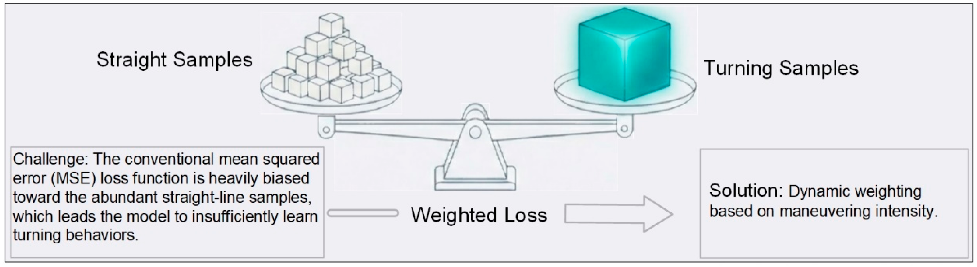
In the task of vessel trajectory prediction, the contribution of individual training samples to the model’s learning objective is non-equivalent. In steady-state straight sailing scenarios, vessel motion patterns are relatively simple and dominated by inertial translation, resulting in low prediction complexity. In contrast, under maneuvering conditions such as turning, yawing, or speed variation, vessel motion exhibits distinct non-linear characteristics, imposing higher demands on the model’s capabilities for temporal modeling and dynamic understanding. However, in real-world engineering datasets, steady-state straight samples typically constitute the vast majority, whereas high-dynamic maneuvering samples exhibit a pronounced long-tailed distribution. Relying solely on the conventional Mean Squared Error (MSE) as the training objective causes parameter updates to be dominated by the multitude of simple samples, leading to insufficient attention to maneuvering behaviors that are critical for navigational safety and decision-making.

To address this, we propose a Dynamic Maneuver-Aware Loss Function. The core philosophy is to adaptively adjust the gradient contribution of training samples based on their maneuvering intensity, without altering the regression target. By explicitly differentiating between steady navigation and high-dynamic maneuvering samples, this loss function guides the model to pay more attention to maneuvering samples with complex trajectory shapes and high prediction difficulty during the training process. Consequently, this effectively mitigates the training bias induced by the long-tailed distribution, ensuring that the model captures critical dynamic behaviors.

Therefore, we introduced a dynamic sample weighting mechanism based on trajectory curvature during the training phase, as illustrated in Figure 2, the “maneuvering intensity” indicator $D_i$ of sample $\mathrm{i}$ is defined as the cumulative heading change in the vessel within the predicted horizon. For the future trajectory sequence $Y_i=\{p_1,p_2,...,p_H\}$ of the i-th sample, calculate the instantaneous heading angle ${\psi }_t$ for each step:

$${\psi }_t=arctan2(y_{t+1}-y_t,x_{t+1}-x_t)$$

(5)

Furthermore, the dynamic gradient weight $w_i$ of the sample is calculated using the following formula:

$$D_i={\displaystyle \frac{1}{H-1}}\sum _{t=1}^{H-1}\Vert {\psi }_{t+1}\ominus {\psi }_t\Vert$$

(6)

Among them, $\ominus$ represents the minimum angle difference operation for handling periodic angle jumps (such as $359^{\circ }\to 1^{\circ }$). The larger the $D_i$, the more curved the vessel’s path and the stronger its maneuverability. Based on this, the dynamic gradient weight $w_i$ is designed as follows:

$$w_i=1.0+\alpha \cdot \tanh (\beta \cdot D_i)$$

(7)

where $\alpha$ denotes the maximum gain coefficient (configured to yield a maximum weight of 5.0), and $\beta$ represents the sensitivity coefficient. The hyperbolic tangent function ($\tanh$) is employed to smoothly map the weights onto the interval $[1,1+\mathsf{\alpha }]$, thereby effectively preventing training instability induced by extreme outliers. Consequently, the final total loss function is formulated as:

$$\mathcal{L}={\displaystyle \frac{1}{N}}\sum _{i=1}^N{w}_i\cdot \Vert {\widehat{Y}}_i-Y_i{\Vert }_2^2$$

(8)

where $N$ denotes the training batch size, while ${\widehat{Y}}_i$ and $Y_i$ represent the predicted trajectory sequence and the corresponding ground truth trajectory sequence for the i-th sample, respectively. Through this mechanism, the model effectively amplifies the relative weight of high-dynamic maneuvering samples during parameter updates, significantly enhancing the precision in capturing non-linear maneuvering behaviors.

In this section, the selection of values for $\alpha$ and $\beta$ is primarily governed by constraints regarding gradient stability and engineering controllability. Specifically,$\alpha$ serves to cap the maximum amplification ratio of high-maneuver samples during parameter updates, preventing a minority of extreme outliers from dominating the training process; whereas $\beta$ modulates the response interval of the weight function to variations in maneuvering intensity, ensuring a smooth and continuous transition of weights from steady-state navigation to high-dynamic maneuvering.

The aforementioned weight allocation mechanism, which calculates the cumulative heading change based on future ground-truth trajectories, is a strictly offline training mechanism. During the model training phase, this mechanism utilizes known future ground-truth data as a modulator for the supervisory signal, compelling the network to learn and memorize complex non-linear maneuvering features. Conversely, during the model deployment and online inference phases, the prediction process relies exclusively on historical observation sequences (AIS and IMU inputs) without any dependence on future information. This design effectively enhances the model’s sensitivity to maneuvering intentions without increasing the computational burden of online inference. Furthermore, this weight calculation formula based on future ground-truth trajectories may introduce potential bias, as it is highly dependent on the quality of the ground-truth data. If the raw AIS or GNSS data exhibits severe positioning drift or high-frequency noise in certain straight-sailing segments, the formula might misclassify them as high-intensity maneuvers and assign unreasonably high weights. It is precisely to address this issue that this paper introduces the saturation characteristics of the tanh function alongside a maximum weight upper bound $\alpha$. This implements a physical truncation of such abnormally high weights at the algorithmic level, thereby suppressing the risk of noise amplification. Despite this potential bias, in practical engineering applications, this offline weighting strategy—which trades the sacrifice of a negligible minority of anomalous noise conditions for a substantial improvement in overall maneuvering prediction accuracy—is highly rational.

3.5. Horizon-Adaptive Scenario Segmentation

In the performance assessment of vessel trajectory prediction models, standard practice involves categorizing samples into distinct motion scenarios—such as straight sailing and turning—based on the magnitude of heading change within the prediction horizon, followed by a separate statistical analysis of prediction errors. However, existing studies predominantly employ a fixed heading threshold (e.g., 10°) for scenario classification, failing to explicitly account for the impact of the prediction horizon length on the maneuver determination scale.

In reality, as dynamic entities characterized by significant inertia, the process of vessel heading change exhibits a pronounced time-scale dependency: within a short prediction horizon, even a minor heading variation may correspond to high-frequency, rapid maneuvering behaviors; conversely, over a longer prediction horizon, an equivalent magnitude of heading change often signifies merely a slow, gradual course adjustment. Adopting a unified fixed threshold for scenario classification is prone to misclassifying genuine maneuvers as straight sailing in short-term predictions, or misinterpreting slow turns as straight conditions in long-term predictions, thereby diminishing the discriminative power of the evaluation results regarding the model’s maneuvering prediction capability. To comprehensively assess model performance across different time scales, this paper proposes a Horizon-Adaptive Scenario Segmentation Strategy. This strategy dynamically adjusts the turning determination threshold according to the prediction horizon length, aligning the scenario classification scale with the inherent time scale of the prediction task. For a given prediction horizon $T_{pred}$ (in seconds), the heading angle threshold ${\theta }_{thres}$ for determining whether a sample constitutes a turning condition is defined as:

$${\theta }_{thres}=\max \left(0.5^{\circ }, 10^{\circ }\times {\displaystyle \frac{T_{pred}}{180}}\right)$$

(9)

In this formulation, the turning determination threshold decreases linearly as the prediction horizon shortens, with a lower bound of $0.5^{\circ }$ explicitly imposed to filter out sensor background noise. This dynamic segmentation strategy ensures that the evaluation metrics precisely capture valid maneuvering behaviors across varying time scales. Consequently, it effectively prevents short-term minor fluctuations from being misclassified as turns, while simultaneously precluding the misidentification of long-term gradual turns as straight sailing conditions.

3.6. Post-Processing Mechanism

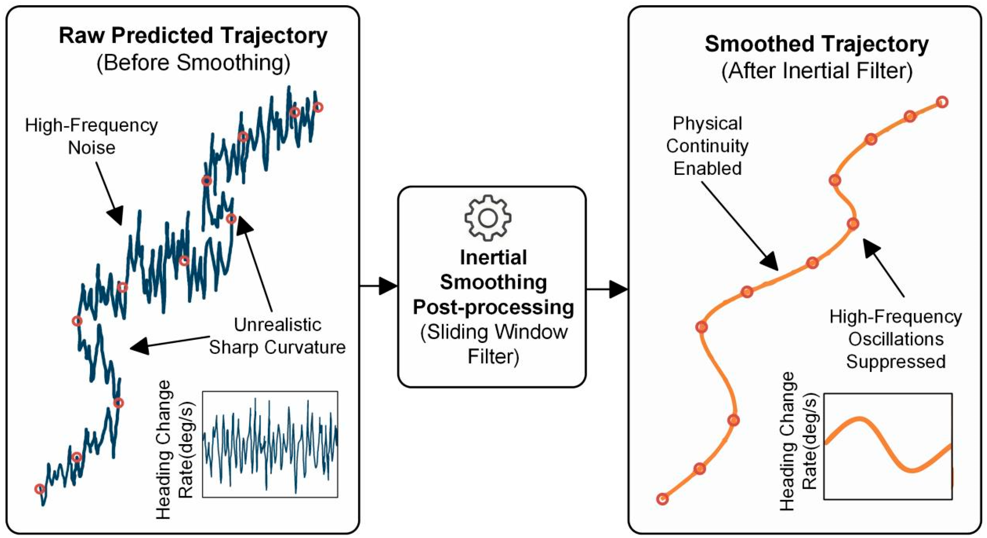
While deep learning models excel at capturing the non-linear mapping relationships between historical observations and future trajectories, their raw outputs often exhibit physical inconsistencies when applied in engineering contexts. Specifically, subject to training data noise, normalization errors, and the intrinsic regression characteristics of the model, prediction results frequently suffer from local high-frequency jitter or abrupt curvature changes. Although these discontinuous or non-smooth trajectory artifacts may be negligible in terms of numerical error metrics, they often lack explicit physical feasibility in the context of actual vessel motion and autonomous collision avoidance decision-making, thereby compromising the engineering usability and safety reliability of the prediction results.

From the perspective of vessel maneuvering hydrodynamics, a vessel constitutes a large inertia system. Its evolution in position and heading inherently possesses significant temporal continuity and curvature smoothness; rapid mutations in speed or course are physically impossible within short time intervals. To correct the non-physical jitter and drift in the model output that violate this physical law, the domain of classical trajectory processing conventionally relies on the Extended Kalman Filter (EKF) and its derivative algorithms [38], alongside data assimilation and smoothing techniques based on Back and Forth Nudging [39,40]. These methods excel in short-term state estimation and smoothing. Serving as a complement to the long-term prediction results of deep learning, imposing moderate physical constraints on predicted trajectories—without introducing external control inputs—effectively enhances their consistency with actual vessel motion laws. Guided by these considerations, as illustrated in Figure 3, this paper introduces an inertially constrained post-processing smoothing mechanism during the inference phase. This mechanism is designed to suppress non-physical high-frequency noise generated by the deep network, thereby augmenting the usability and stability of the predicted trajectories in practical engineering scenarios.

We employ a sliding window technique (Window Size = 30 s) to perform mean filtering on the predicted coordinate sequence, aiming to suppress high-frequency jitter induced by sensor background noise. The formulation is expressed as:

$${\widehat{P}}_t={\displaystyle \frac{1}{w}}\sum _{i=-w/2}^{w/2}{P}_{t+i}$$

(10)

where $w$ denotes the size of the sliding window (set to 30 in this experiment), and $P$ represents the raw predicted coordinate. This procedure effectively eliminates quantization noise arising from the discretization of AIS data, rendering the generated trajectory more consistent with vessel kinematic characteristics.

To ensure absolute fairness in model evaluation, the aforementioned smoothing post-processing step is uniformly applied to all physics baseline models and deep learning models (including both single-modal and multimodal architectures) across all comparative experiments in this study. Regarding its impact on evaluation metrics, the primary function of this smoothing step is to suppress non-physical high-frequency oscillations within the predicted trajectories. Consequently, its influence on the whole-process Average Displacement Error (ADE) and Final Displacement Error (FDE) is relatively marginal, as it does not alter the macroscopic evolution direction or the long-term trend of the trajectory. In other words, this filtering effect serves merely as a physical safeguard for trajectory continuity; it cannot fundamentally rectify long-term trajectory divergence arising from the model’s inadequate early maneuver perception capability. The decoupling and quantification of the respective contributions to performance enhancement from the deep network’s multimodal fusion mechanism and the post-processing filtering effect will be comparatively discussed in the subsequent cross-ablation experiments (detailed in Section 5.2).

4. Experimental Description

To comprehensively evaluate the effectiveness of the proposed framework in practical engineering scenarios—particularly its robustness under conditions of data sparsity and large-angle turning maneuvers—comparative experiments were conducted utilizing data collected from real-vessel sea trials. This section details the construction of the experimental dataset, the configuration of baseline models, and the specific evaluation metrics employed.

4.1. Experimental Platform and Data Acquisition

The data acquisition for this study relies on real-vessel sea trials. The experimental environments encompass a variety of typical operating conditions, ranging from open-water cruising to inland river navigation in the Beijing–Hangzhou Grand Canal. A Fiber-Optic Gyroscope Inertial Navigation System (FOG-INS) was employed for the experiments. This system is capable of outputting raw IMU data at a frequency of 100 Hz and providing integrated navigation parameter reference values. Detailed technical specifications of the equipment are presented in

Table 2. Technical specifications of the IMU used in the experiments.

Parameters		Values
Sampling rate		100 Hz
Accelerometers	Range	±10 g
	Bias	0.07 mg
Gyroscopes	Range	$\pm 1000°/\mathrm{s}$
	Bias	$0.5°/\mathrm{h}$
	Random walk	$\le 0.5°/\sqrt{\mathrm{h}}$

. Regarding data processing, a post-processing approach based on real-time acquisition mode was adopted.

To validate the model’s robustness under small-sample and long-tailed distribution conditions, we performed a quantitative statistical analysis on the collected real-ship data. After applying the kinetic threshold filtering (<2.0 kn), the final dataset comprises a total effective navigation duration of approximately 6.0 h, yielding 21,697 continuous trajectory sequences using the sliding window approach. The statistical results indicate an extreme long-tailed distribution characteristic: steady-state straight-sailing samples (with a cumulative heading change of less than 10°) heavily dominate the dataset, accounting for 80.3%, whereas dynamic maneuvering samples account for merely 19.7%.

Furthermore, instead of a conventional random shuffle, we adopted a strict chronological splitting strategy. The earlier continuous voyages were used as the training set (accounting for approximately 90.5%), while the final trajectory segments were held out entirely as the test set (accounting for 9.5%). This chronological split ensures no future information leakage and naturally introduces a “Distribution Shift.” Because the test set contains specific complex maneuvers that are under-represented in the training phase, this data splitting strategy provides a rigorous engineering benchmark for evaluating the effectiveness of our dynamic maneuver-aware loss and multimodal fusion mechanism.

4.2. Baseline Models and Comparative Experimental Setup

To precisely quantify the contribution of the Inertial Measurement Unit (IMU) to trajectory prediction and validate its effectiveness in enhancing accuracy during non-linear maneuvers, a controlled variable experiment was designed. To ensure the fairness of comparison, all models described below (including both single-modal and multimodal fusion models) are trained and tested based on the unified data preprocessing pipeline described in Section 3.2, sharing identical kinetic energy filtering thresholds and offline parameter locking normalization parameters.

(1) Linear Extrapolation Model (Physics Baseline): A physics-based model relying on the instantaneous motion state. This model utilizes the average velocity and heading vectors within a sliding window (past 10 s) to perform tangential prediction. It incorporates no data-driven non-linear modeling capabilities. This baseline serves to characterize the baseline error level achievable in straight and turning scenarios when relying solely on local kinematic information. It is worth noting that although methods like the Extended Kalman Filter (EKF) exhibit excellent performance in state estimation tasks, their primary objective lies in current state filtering rather than long-term future trajectory prediction. Given that this study focuses on the capability of data-driven models to model motion trends over long prediction horizons, the linear extrapolation model is adopted as the representative lower bound for physics-based methods.

(2) Single-modal Ablation Group: This group is designed to evaluate the prediction capability of models relying exclusively on AIS kinematic information. They maintain an identical backbone network architecture, loss function weights, and parameter configurations to the proposed fusion models. The sole distinction lies in the removal of the IMU dynamic feature branch at the input layer. Specifically, this group includes: Transformer (No-IMU): A self-attention model based solely on AIS position, speed, and heading features. It is used to assess the modeling capability of the attention architecture for complex maneuvering scenarios under high-quality preprocessing conditions; LSTM (No-IMU): A recursive model based solely on AIS inputs. As a classical time-series prediction benchmark, it is used to analyze the error accumulation characteristics of recursive structures in long-term prediction when dynamic constraints are absent.

(3) Multimodal Fusion Models: Building upon the aforementioned single-modal models, this group incorporates dynamic features such as acceleration and angular velocity provided by the IMU. These models are used to evaluate whether fusing inertial information can enhance the model’s perception of vessel maneuvering changes and improve trajectory prediction stability and precision under identical data quality and model structure conditions. Specifically, this group includes: Transformer (Full): An attention model fusing AIS and IMU features; LSTM (Full): A recursive model fusing AIS and IMU features.

Through this multi-level comparative experimental design, we systematically analyze the impact of different model structures and input modalities on vessel trajectory prediction performance within a unified experimental framework. It is important to emphasize that the comparative design in this study does not seek to maximize the performance of a single model in isolation, but rather, through strict variable control, to evaluate the specific impact of introducing IMU dynamic information on prediction stability and maneuver perception capability under practical engineering constraints.

4.3. Evaluation Metrics

To quantitatively evaluate the prediction performance under different prediction horizons, the Average Displacement Error (ADE) and Final Displacement Error (FDE) are adopted as the primary evaluation metrics. Both metrics are ultimately reported in meters. As the original data are represented in geographic coordinates (latitude and longitude), the Haversine great-circle distance is employed to eliminate projection distortions induced by the Earth’s curvature. Specifically, the distance computation consists of two steps. First, the great-circle distance is calculated in nautical miles, followed by a unit conversion to meters. For a predicted position $p^{Pred}({\varphi }_p,{\lambda }_p)$ and the corresponding ground-truth position $p^{GT}({\varphi }_g,{\lambda }_g),$ the spherical distance $d_{NM}\left(t\right)$ (in nautical miles) between the two points is computed by converting the latitude and longitude from degrees to radians as:

$${\varphi }^{\prime }=\varphi {\displaystyle \frac{\pi }{180}}, {\lambda }^{\prime }=\lambda {\displaystyle \frac{\pi }{180}}$$

(11)

$$a={\sin }^2\left({\displaystyle \frac{{\varphi }_p^{\prime }-{\varphi }_g^{\prime }}{2}}\right)+\cos ({\varphi }_g^{\prime })\cdot \cos ({\varphi }_p^{\prime })\cdot {\sin }^2\left({\displaystyle \frac{{\lambda }_P^{\prime }-{\lambda }_P^{\prime }}{2}}\right)$$

(12)

$$d_{NM}=2R_{nm}\cdot \arcsin \left(\min (1,\sqrt{a})\right)$$

(13)

where $\varphi$ and $\lambda$ denote the latitude and longitude expressed in radians, respectively, and $R_{nm}\approx 3440$ represents the Earth’s radius in nautical miles. The obtained distance is then converted into physical distance (meters) using the internationally standardized conversion factor:

$$Erro{r}_m=d_{NM}\times 1852$$

(14)

ADE quantifies the average trajectory fitting accuracy of the model over the entire prediction horizon, characterizing the model’s capability to capture the overall vessel motion trend; whereas FDE evaluates the positional deviation at the final prediction timestamp $T$ (e.g., $T=180 s$) primarily highlighting the cumulative error level in long-term predictions:

$$\mathrm{ADE}={\displaystyle \frac{1}{N}}\sum _{i=1}^N{\displaystyle \frac{1}{T}}\sum _{t=1}^T{Error}_m^{\left(i\right)}(T)$$

(15)

$$\mathrm{FDE}={\displaystyle \frac{1}{N}}\sum _{i=1}^N{Error}_m^{\left(i\right)}(T)$$

(16)

where $N$ denotes the total number of samples in the test set. This evaluation framework not only eliminates geometric distortion induced by geographic projection but also strictly adheres to the “nautical mile-to-meter” metric conversion standards prevalent in maritime engineering, thereby ensuring the engineering applicability of the experimental results. Furthermore, to investigate the model’s robustness under non-linear maneuvering conditions, we partitioned the test set into two subsets—steady-state straight sailing and dynamic turning—based on the adaptive threshold ${\theta }_{thres}$ defined in Section 3.5, for separate evaluation. This scenario-segmented evaluation strategy effectively prevents the dominating influence of straight-line samples from masking the model’s true performance in critical turning scenarios.

5. Experimental Results and Analysis

This section analyzes model performance from three dimensions: overall prediction accuracy, scenario-specific robustness (straight sailing vs. turning), and ablation studies. Experimental results demonstrate that under conditions of data sparsity, deep learning models outperform traditional physics-based extrapolation baselines. Furthermore, the introduction of IMU physical features significantly mitigates the prediction lag observed in AIS-only models during the maneuver initiation phase and effectively suppresses cumulative errors in long-term predictions.

5.1. Comparative Analysis: Physics Baseline and Deep Learning

To validate the necessity of data-driven methods in practical engineering, this section compares the performance of the Physics Baseline against the Multimodal Fusion Models (Transformer-Full/LSTM-Full) under different operating conditions. By combining quantitative metrics with qualitative visualization, this section clearly delineates the performance boundaries between physical models and deep learning models.

5.1.1. Straight Scenarios

In steady-state straight sailing conditions, variations in vessel heading and speed are gradual, and the motion behavior approximately satisfies the assumption of uniform linear motion. The Physics Baseline model, by performing linear extrapolation based on short-term average speed and heading, can theoretically achieve lower prediction errors. In contrast, deep learning models require inference based on learned motion patterns, and their performance may be compromised by model complexity and data noise. Therefore, the comparative results in straight sailing scenarios serve to clarify the performance trade-off of deep learning methods relative to physical models and to verify whether the multimodal fusion strategy introduces unnecessary error amplification. Based on these considerations, this paper presents a comparative analysis of the Average Displacement Error (ADE) between the Physics Baseline and the IMU-integrated Multimodal Deep Learning Models (Transformer-Full and LSTM-Full) across different prediction horizons.

As presented in

Table 3. Comparison of ADE in straight scenarios.

Horizon	Baseline	Transformer (Full)	LSTM (Full)
30 s	2.73 m	7.76 m	6.31 m
60 s	5.67 m	21.14 m	8.91 m
90 s	9.03 m	22.45 m	10.52 m
120 s	12.12 m	51.07 m	18.61 m
150 s	20.49 m	31.10 m	19.58 m
180 s	25.17 m	16.86 m	42.02 m

, under steady-state straight sailing conditions, the Physics Baseline model exhibits extremely low Average Displacement Errors (ADE) across multiple prediction horizons, which perfectly aligns with its modeling premise based on the uniform linear motion assumption. In contrast, the multimodal deep learning models yield relatively higher errors at certain prediction horizons. Notably, in such stable navigation scenarios, the error of the Transformer model is significantly higher than that of the LSTM model at specific prediction horizons (e.g., 60 s, 120 s, 150 s), indicating a certain degree of trajectory instability.

This phenomenon profoundly reflects the fundamental differences in “inductive bias” across distinct deep network architectures. As a recurrent neural network, LSTM inherently possesses an inductive bias of “temporal inertia.” The smooth transmission of its hidden states acts as strong regularization; therefore, when confronted with approximately linear, steady-state straight sailing conditions, LSTM manages to maintain high stability. Conversely, the Transformer architecture relies entirely on the global multi-head attention mechanism, discarding strict progressive temporal constraints. Although this extremely high structural degree of freedom endows the Transformer with an exceptional capability to rapidly capture high-frequency, non-linear maneuvering intentions, when processing simple straight-sailing samples lacking dynamic variations, its massive parameter space and dense attention heads are highly susceptible to “overfitting” on local high-frequency sensor noise (e.g., minor hull oscillations induced by waves, high-frequency IMU drift). This excessive allocation of attention to minor noise directly leads to trajectory micro-fluctuations and local error amplification during steady-state extrapolation for the Transformer.

From an engineering application perspective, the Transformer trades a portion of its regularization smoothness during steady-state navigation for extremely high perceptual sensitivity to high-dynamic, hazardous maneuvers. Considering the typical dimensions of merchant vessels and the environmental uncertainties inherent in straight-sailing conditions, error fluctuations in the order of ten meters are acceptable in engineering applications. This indicates that the introduction of IMU attitude information does not induce significant performance degradation in the deep learning models under basic navigation states.

5.1.2. Turning Scenarios

Distinct from the stable performance observed in straight sailing, turning scenarios impose more stringent demands on the model’s maneuver perception capability and non-linear modeling capacity. These scenarios are also more prone to exposing the disparities between different methods regarding physical assumptions and information utilization.

Table 4. Comparison of ADE in turning scenarios.

Horizon	Baseline	Transformer (Full)	LSTM (Full)
30 s	18.34 m	8.99 m	10.03 m
60 s	47.11 m	24.41 m	36.35 m
90 s	105.45 m	48.12 m	55.47 m
120 s	162.98 m	79.35 m	78.08 m
150 s	218.47 m	117.63 m	98.47 m
180 s	287.63 m	167.61 m	154.67 m

and

Table 5. Comparison of FDE in turning scenarios.

Horizon	Baseline	Transformer (Full)	LSTM (Full)
30 s	47.66 m	10.30 m	19.20 m
60 s	129.47 m	35.52 m	90.80 m
90 s	273.91 m	85.29 m	124.52 m
120 s	440.20 m	164.72 m	221.30 m
150 s	549.62 m	283.44 m	244.89 m
180 s	750.62 m	459.93 m	426.07 m

present a comparative analysis of the performance of each model under turning conditions from two perspectives: trajectory fitting accuracy (ADE) and endpoint prediction capability (FDE), respectively.

As shown in Table 4, when the prediction horizon is 60 s, the vessel is typically in the maneuver initiation phase, transitioning from straight sailing to a steady turn. This phase is particularly sensitive to the model’s ability to capture changes in motion trends. At this horizon, the Physics Baseline model, based on the assumption of constant velocity and heading, begins to exhibit kinematic lag, with the ADE accumulating to 47.11 m. In contrast, the Transformer (Full) model, which incorporates IMU dynamic information, successfully captures the early turning intention, constraining the error to 24.41 m. This indicates that during the maneuver initiation phase, introducing dynamic features such as angular velocity helps the model perceive heading change trends earlier, thereby mitigating the rapid growth of prediction error. Furthermore, the fusion model demonstrates a distinct advantage in Final Displacement Error (FDE) (see Table 5). Its error growth trend is significantly lower than that of the Physics Baseline, further suggesting that IMU dynamic information contributes to synchronously improving both process-fitting accuracy and endpoint prediction stability during the initial maneuvering stage.

As the prediction horizon extends to 180 s, discrepancies in long-term motion trend modeling become more pronounced. As shown in Table 5, the FDE of the Physics Baseline grows rapidly with prediction time, ultimately reaching 750.62 m. This indicates that during long-term non-linear maneuvers, extrapolation methods based on local linear assumptions fail to maintain trajectory prediction validity, thereby losing their engineering reference value. In contrast, although multimodal fusion models are also subject to error accumulation, the LSTM (Full) fusion model manages to constrain the FDE to 426.07 m, representing a 43.2% reduction compared to the Physics Baseline. From the perspective of process error (ADE), while the average error of all models accumulates as the horizon extends, the growth rate of the multimodal fusion model is significantly lower than that of the Physics Baseline. This aligns with its performance trend in FDE, demonstrating its ability to globally suppress error diffusion and exhibiting stronger stability in long-term predictions.

Synthesizing the ADE and FDE comparison results reveals that the primary limitation of the Physics Baseline lies in its inability to cope with the continuous accumulation of errors during non-linear maneuvers. Conversely, by introducing real-time dynamic constraints provided by the IMU, the multimodal fusion model improves maneuver perception capability at the turn initiation stage and effectively suppresses the divergence trend along the tangential direction in long-term predictions, thereby demonstrating superior robustness under complex navigation conditions.

To further intuitively analyze the differences in prediction behavior across models under turning conditions and to corroborate the aforementioned quantitative metric results, two representative right-turn maneuvering samples were selected for a visual comparison of trajectory results from different prediction methods over medium-to-long prediction horizons. Figure 4 and Figure 5 illustrate the relationship between predicted trajectories and the ground truth tracks at prediction horizons of 120 s and 180 s, respectively. In the figures, the grey curve represents the historical trajectory, the black marker denotes the ground truth endpoint, the green dashed line indicates the physics extrapolation result based on instantaneous motion state, the orange curve depicts the predicted trajectory of the single-modal model using AIS data only, and the red curve represents the prediction result of the multimodal model fusing IMU dynamic features.

As illustrated in Figure 4, at the 120 s prediction horizon, the Physics Baseline model continues to extrapolate along the pre-turn tangential heading, failing to reflect the actual heading changes that occurred. This leads to a significant deviation of the predicted trajectory from the ground truth track, a phenomenon that aligns with the results of rapid ADE accumulation under turning conditions shown in Table 4. In contrast, the Single-modal AIS model is capable of capturing the overall trend of the vessel’s right turn. Although it achieves reasonable performance in terms of endpoint FDE, notable discrepancies remain in turning magnitude and curvature during the initial phase of the turn, causing the overall trajectory to differ considerably from the ground truth. Conversely, the Multimodal Fusion model, incorporating IMU information, demonstrates a timelier response to heading changes during the initial turning phase, yielding a predicted trajectory that is morphologically closer to the ground truth.

Further observation of the 180 s long-term prediction results in Figure 5 reveals that the trajectory of the Physics Baseline has diverged significantly along the tangential direction. A substantial offset exists between its endpoint and the ground truth, which is consistent with the trend of sharp increase in FDE for the Physics Baseline over long prediction horizons as shown in Table 5. While the Single-modal AIS model mitigates error diffusion to a certain extent, it still exhibits evident cumulative drift. In comparison, the Multimodal Fusion model, subject to physically constrained post-processing, maintains high consistency between its predicted trajectory and the ground truth in terms of the overall trend, highlighting its stability advantage in long-term non-linear maneuvering prediction.

Synthesizing the results from quantitative metrics and qualitative trajectory comparison, it is evident that the introduction of IMU dynamic information not only improves the model’s maneuver perception capability during the maneuver initiation phase but also effectively suppresses the tangential divergence trend in long-term predictions, thereby providing more reliable engineering support for trajectory prediction under complex navigation conditions.

5.2. Ablation Study: The Critical Role of IMU Data

To precisely quantify the respective contributions of the Inertial Measurement Unit (IMU) dynamic information and the smoothing post-processing mechanism to trajectory prediction, and to prevent ambiguous attribution of performance gains caused by inter-module coupling, this section introduces a cross-ablation study encompassing different input modalities (Full vs. No-IMU) and the application of post-processing (Full vs. No-Smoothing). The ablation experiments reveal three critical phenomena: first, the “maneuvering blind zone” effect exhibited by pure-AIS models during the 60 s short-term prediction; second, the smoothing post-processing functions merely as an auxiliary mechanism to ensure the physical continuity of the trajectory; and third, even when completely decoupling the smoothing post-processing, IMU features continue to play a decisive role in enhancing long-term prediction accuracy.

5.2.1. Elimination of the 60 s Maneuvering Blind Zone

Based on the preceding analysis, the 60 s prediction horizon corresponds to the maneuver initiation phase. During this phase, the vessel has not yet fully entered steady-state turning but has already deviated from the assumption of pure straight sailing, making it a critical temporal scale for evaluating the model’s maneuver perception capability. Consequently, this section focuses on a comparative assessment of model performance at this specific horizon.

Table 6. Results of IMU ablation study under turning conditions (ADE comparison).

Horizon	Baseline	Transformer (No-IMU)	Transformer (No-Smoothing)	Transformer (Full)	LSTM (No-IMU)	LSTM (No-Smoothing)	LSTM (Full)
30 s	18.34 m	12.29 m	8.63 m	8.99 m	8.18 m	10.45 m	10.03 m
60 s	47.11 m	175.77 m	24.92 m	24.41 m	143.21 m	37.67 m	36.35 m
90 s	105.45 m	58.11 m	48.48 m	48.12 m	62.76 m	53.87 m	55.47 m
120 s	162.98 m	91.81 m	79.22 m	79.35 m	108.98 m	79.87 m	78.08 m
150 s	218.47 m	140.86 m	120.13 m	117.63 m	142.12 m	97.64 m	98.47 m
180 s	287.63 m	203.80 m	168.15 m	167.61 m	201.72 m	157.84 m	154.67 m

and

Table 7. Results of IMU ablation study under turning conditions (FDE comparison).

Horizon	Baseline	Transformer (No-IMU)	Transformer (No-Smoothing)	Transformer (Full)	LSTM (No-IMU)	LSTM (No-Smoothing)	LSTM (Full)
30 s	47.66 m	17.47 m	10.96 m	10.30 m	18.75 m	19.61 m	19.20 m
60 s	129.47 m	354.33 m	38.14 m	35.52 m	305.91 m	93.17 m	90.80 m
90 s	273.91 m	86.37 m	85.44 m	85.29 m	133.30 m	122.61 m	124.52 m
120 s	440.20 m	197.86 m	165.91 m	164.72 m	271.57 m	220.30 m	221.30 m
150 s	549.62 m	310.05 m	285.95 m	283.44 m	348.75 m	252.05 m	244.89 m
180 s	750.62 m	464.58 m	461.94 m	459.93 m	497.66 m	428.73 m	426.07 m

present the ADE and FDE comparison results, respectively, for the IMU ablation study under turning conditions.

It is evident that at the 60 s prediction horizon, all single-modal models with IMU features removed exhibited substantial performance deterioration. The ADE of the Transformer (No-IMU) and LSTM (No-IMU) escalated to 175.77 m and 143.21 m, respectively, while their corresponding FDEs reached 354.33 m and 305.91 m. In contrast, the fusion models incorporating IMU dynamic information significantly reduced both process and endpoint errors under the same prediction horizon, demonstrating superior prediction stability. It is noteworthy that, even when the smoothing post-processing is completely stripped away, the ADE and FDE at the 60 s prediction horizon remain substantially lower than those of the baseline models without IMU fusion. This directly demonstrates that the performance leap of the multimodal model during the maneuver initiation phase fundamentally stems from the model’s deep learning of IMU features and its perception of maneuvering intent. To intuitively describe this phenomenon, Figure 6 illustrates the underlying causes.

The figure indicates that when a vessel just enters the initial phase of a turn, its historical positional trajectory remains predominantly linear in morphology. Models relying solely on kinematic information such as position, speed, and heading struggle to timely perceive the trend of heading change. Due to the vessel’s large mass inertia, the AIS-derived trajectory has not yet exhibited distinct curvature at this stage. Consequently, single-modal models tend to persist with the straight-line assumption, leading to prediction failure. Conversely, multi-modal models equipped with IMU data anticipate changes in angular velocity and acceleration, thereby reflecting the vessel’s maneuvering intention and enhancing prediction precision.

Further trajectory comparison results are presented in Figure 7. In this sample, the predicted trajectory of the single-modal model is visibly biased towards linear extrapolation during the maneuver initiation phase, resulting in a large deviation from the ground truth track. However, by incorporating angular velocity and acceleration information provided by the IMU, the multimodal fusion model transforms the prediction paradigm from “reactive response” to “proactive perception.” Its predicted trajectory can deviate from the linear trend earlier to respond to turning behaviors, effectively controlling error growth within the 60 s horizon.

Synthesizing the tabular data and visualization results, it is evident that the failure of single-modal models using AIS data during the maneuver initiation phase is not due to insufficient training or limited model capacity, but is primarily constrained by the physical observability of the input information. IMU dynamic information provides critical supplementary perception at this stage, enabling the model to bridge the maneuvering blind zone caused by kinematic observational lag.

5.2.2. Significant Improvement in Process Safety

In long-term predictions (T > 120 s), the focus of model evaluation should shift from the singular Final Displacement Error (FDE) to the Average Displacement Error (ADE) over the entire process. This is because, in the context of maritime collision avoidance decision-making, the “shape fidelity” of the trajectory is more critical than “endpoint accuracy.” As long as the predicted trajectory correctly reflects the vessel’s turning trend, it can effectively trigger collision warnings, whereas the longitudinal positional deviation at the endpoint has a relatively minor impact on the collision avoidance geometry.

As evidenced by the results in Table 6, at the 180 s prediction horizon, the introduction of IMU dynamic features leads to a stable and significant improvement in the model’s whole-process error. Specifically, the ADE of the Transformer (No-IMU) is 203.80 m, while fusing IMU data reduces it to 167.61 m, representing an error reduction of 17.8%. The improvement in the LSTM architecture is even more pronounced, with its ADE decreasing from 201.72 m to 154.67 m, an overall enhancement of approximately 23.3%. Furthermore, the cross-ablation data further demonstrate that the Transformer (No-Smoothing) yields an ADE of 168.15 m at the 180 s horizon. This value is not only remarkably close to the finally smoothed result of 167.61 m, but also remains substantially lower than the 203.80 m of the pure-AIS model. The LSTM model exhibits an identical performance trend. This result indicates that in long-term predictions, the angular velocity and acceleration information provided by the IMU can continuously constrain the direction of trajectory evolution, effectively suppressing the cumulative diffusion of error in the temporal dimension, whereas the smoothing mechanism merely performs marginal numerical denoising upon this foundation.

In contrast, data in Table 7 indicates that the difference in endpoint error (FDE) between single-modal and multimodal models at 180 s is relatively limited. This is primarily attributed to the inevitable cumulative drift in long-term predictions and the inherent integration errors of the sensors themselves. However, the significant advantage in ADE demonstrates that the IMU successfully constrains the intermediate process of the trajectory, ensuring it maintains a curvature trend consistent with the actual track throughout. This “process consistency” guarantees that the model provides a physically credible collision avoidance reference across the entire time domain (0–180 s), thereby offering a reference trajectory with higher physical credibility and engineering utility for long-term decision-making.

5.3. Discussion on the Limitations of the Proposed Method

Although the multimodal fusion framework proposed in this paper demonstrates excellent robustness under sparse data conditions, certain limitations remain, which necessitate further exploration in future work:

(1)

Limitations of Experimental Data and Conclusion Generalizability: This study experimentally proves that introducing IMU data significantly improves performance during prediction phases prone to maneuvering lag, and the multimodal fusion model effectively compensates for the maneuver perception blind zone within a prediction horizon of approximately 60 s. However, the specific timing of this blind zone (e.g., 60 s, 80 s, or other time scales) may be influenced by multiple factors, including vessel motion state, vessel dimensions, propulsion methods, and the data acquisition environment. Consequently, the generalizability of the conclusion regarding the specific time scale has certain defects and requires further systematic verification on larger-scale datasets covering multiple vessel types.

(2)

Limitations of Operating Condition Coverage: The current experimental data were primarily collected from the navigation processes of a single vessel in open waters and the Beijing–Hangzhou Grand Canal. While large-angle turning maneuvers are included, complex scenarios such as multi-vessel encounters or operations of vessels with different tonnages have not yet been covered. However, it is important to note that the focus of this study is not to construct a cross-vessel generalized model, but to reveal the physical observability limitations of AIS at the maneuver initiation phase from the perspective of sensor modalities. This conclusion is independent of specific vessel types and possesses universal engineering significance.

(3)

Simplification of Environmental Interference: This study mainly focuses on the handling of internal sensor noise (e.g., IMU drift), with insufficient consideration given to the indirect impact of extreme sea conditions (e.g., severe hull rolling/pitching caused by strong winds and waves) on the reception quality of AIS-related data signals.

(4)

Model Generalizability: The current distribution alignment parameters are set based on the dynamic characteristics of a specific vessel. For vessels with different tonnages or propulsion systems, these prior parameters may need to be readapted or optimized using transfer learning.

6. Conclusions

To address the issue of insufficient accuracy in vessel trajectory prediction under sparse data conditions, this paper proposes a multimodal deep learning prediction framework fusing AIS and IMU information, and conducts systematic experimental validation based on real-vessel data. The following conclusions are drawn: (1) By employing offline parameter locking based on domain priors and weighted loss training oriented towards maneuvering samples, the problem of model divergence under small-sample conditions is successfully resolved, achieving robust trajectory prediction performance. (2) Vessel trajectory prediction relying solely on AIS kinematic information suffers from an inevitable physical blind zone during the maneuver initiation phase. This issue stems from the lag in kinematic observation rather than algorithmic deficiencies. The high-frequency dynamic information provided by the IMU significantly enhances the model’s capability to perceive early maneuvering intentions, thereby effectively mitigating the prediction lag phenomenon. (3) Multimodal fusion not only bridges this physical blind zone but also significantly enhances the shape fidelity of the trajectory in 180 s long-term predictions by reducing the Average Displacement Error (ADE). It achieves a long-term robustness superior to the single-modal AIS model by 23.3% and the physics baseline by 46.2%. The research results indicate that in safety-critical scenarios for practical marine engineering applications, the IMU should not be regarded as an optional auxiliary sensor, but as a core component of the vessel trajectory prediction system.

Furthermore, although this study primarily focuses on the micro-level task of ship trajectory prediction, its practical engineering value extends significantly to macro-level maritime operational analyses. As demonstrated by recent studies on maritime operations (such as the demurrage pattern analysis by Kweon et al. [9]), AIS-based motion analysis is crucial for identifying issues such as delay propagation, berth congestion, and vessel underutilization. By overcoming kinematic lag and accurately predicting complex maneuvering intentions over extended temporal horizons, our proposed multimodal fusion framework can directly support these downstream operational decisions. Ultimately, the enhanced predictive performance not only facilitates immediate collision avoidance but also contributes to broader operational applications, including berth allocation optimization, congestion mitigation, and demurrage risk management.

Future work will further systematically verify the universality and applicability boundaries of the conclusions through data experiments expanded to multiple vessel types, operating conditions, and navigation environments. Concurrently, we will explore the introduction of attention mechanisms to enhance the adaptive utilization of IMU features, and combine transfer learning and few-shot learning methods to further reduce the model’s dependence on large-scale labeled data.