Article

Preliminary Evaluation of Geothermal Potential in Offshore Depleted Petroleum Reservoirs: The Prinos-Kavala Basin, Northern Aegean, Greece


by
Adamantia Raftogianni
1,
Ioannis Vakalas
1,2,*,
Paschalia Kiomourtzi
3,
Yannis Tsiantis
3,
George Apostolopoulos
1,
Francesca Pace
4 and
Vasileios Gaganis
1
1
School of Mining and Metallurgical Engineering, Department of Geological Sciences, National Technical University of Athens, Zografou Campus, Iroon Polytechniou 9 Str., 15773 Athens, Greece
2
Institute of GeoEnergy, Technical University of Crete, 73100 Chania, Greece
3
Energean Oil & Gas, 32, Atrina Center, Kifissias Avenue, 15125 Marousi, Greece
4
Department of Environment, Land and Infrastructure Engineering (DIATI), Politecnico di Torino, Corso Duca degli Abruzzi, 24, 10129 Torino, Italy
*
Author to whom correspondence should be addressed.
J. Mar. Sci. Eng. 2026, 14(5), 421; https://doi.org/10.3390/jmse14050421
Submission received: 19 January 2026 / Revised: 18 February 2026 / Accepted: 22 February 2026 / Published: 25 February 2026
(This article belongs to the Section Marine Energy)

Abstract

The increasing global demand for energy has accelerated the depletion of identified conventional resources, highlighting the need for sustainable alternatives. Geothermal energy, a renewable resource derived from the Earth’s internal heat, offers a reliable solution for both power generation and direct use applications. We present a comprehensive investigation of medium-enthalpy geothermal reservoirs in the Prinos–Kavala Basin, Northern Aegean, Greece. We firstly integrate geological, geophysical, and geochemical data from 66 wells across Prinos–Kavala basin to analyze the temperature distribution in the reservoir. The methodology includes the correction of bottom-hole temperatures and estimation of the geothermal gradients. A 1-D semi-steady-state well temperature modeling technique was applied to estimate the expected production wellhead temperature and assess its suitability for surface heating applications. Results reveal significant spatial heterogeneity in geothermal gradients and reservoir properties, with overpressured conditions confirmed in key zones. The integration of 3D reservoir model and isothermal mapping (>90 °C) identifies zones with high geothermal potential, supporting optimal exploitation strategies. The estimated production wellhead temperatures support the utilization of the produced brine heat content for various applications, among them the pre-heating of a CO2 stream to be injected within the CCS framework for wellbore thermal stress management purposes. The findings demonstrate the value of reservoir characterization for sustainable geothermal development in complex tectonic settings.

1. Introduction

The global transition to renewable energy sources is driven by the urgent need to address the effects of climate change and to ensure energy security. Geothermal energy, harnessed from the Earth’s internal heat, is a sustainable and reliable resource that provides base-load power and direct heating applications. Despite its potential, geothermal exploitation in Greece remains underdeveloped compared to other renewable sources [1].
The Prinos–Kavala Basin in the Northern Aegean is a region of significant geological complexity and geothermal interest. This basin is the offshore extension of the Nestos basin, which is known for its geothermal potential [2,3]. The basin hosts several hydrocarbon reservoirs, with medium enthalpy (90–150 °C) geothermal systems offering promising opportunities for energy production. However, the efficient exploitation of these resources requires detailed reservoir characterization, integrating geological, geophysical, and geochemical data.
In parallel with conventional geothermal development, carbon capture and storage (CCS) has emerged as a critical technology for reducing greenhouse gas emissions [4]. A key operational challenge in CCS projects is the thermal management of CO2 during injection. Injecting cold CO2 into deep formations can lead to significant cooling of the near-wellbore region, causing thermal stress on casing and cement. To mitigate these issues and enhance dissolution of CO2 into formation fluids, several international projects have adopted strategies to heat CO2 prior to injection, ensuring that the injected stream is thermally compatible with the downhole conditions.
Experience from global CCS projects illustrates the importance of thermal considerations within the CO2 storage context. At Sleipner in Norway, thermal modeling was essential to predict plume migration and predict pressure field, under varying temperature conditions [5]. The Quest project in Canada demonstrated the inverse relationship between injectivity index and temperature and that monitoring the geothermal gradient is necessary to assess CO2 loss of containment within the geological store [6]. The Ordos CCS demonstration project in China highlighted how thermal effects influence near-wellbore conditions and long-term reservoir performance [7]. Similarly, reservoir temperature monitoring in injection and observation wells is an integral part of the CO2 plume monitoring at the Tomakomai CCS demonstration in Japan [8]. These lessons are directly relevant to the Prinos Basin, which is being evaluated for CO2 storage as part of Greece’s energy transition strategy [9,10]. Heating CO2 before injection into Prinos reservoirs can reduce thermal shock to well infrastructure. The effects on injectivity are complex and affected by lower viscosity and density contrasts, accelerated trapping mechanisms, and permeability changes due to rock matrix contraction and thermal cracking.
This paper aims to present a comprehensive methodology for the assessment and exploitation of medium enthalpy geothermal reservoirs, focusing on the Prinos–Kavala Basin, while incorporating thermal considerations for CO2 injection and storage. Advanced modeling techniques are employed to evaluate reservoir properties, thermal regimes, and operational strategies, contributing to the broader understanding of geothermal systems and CCS integration.

2. Geological Setting

2.1. Regional Setting

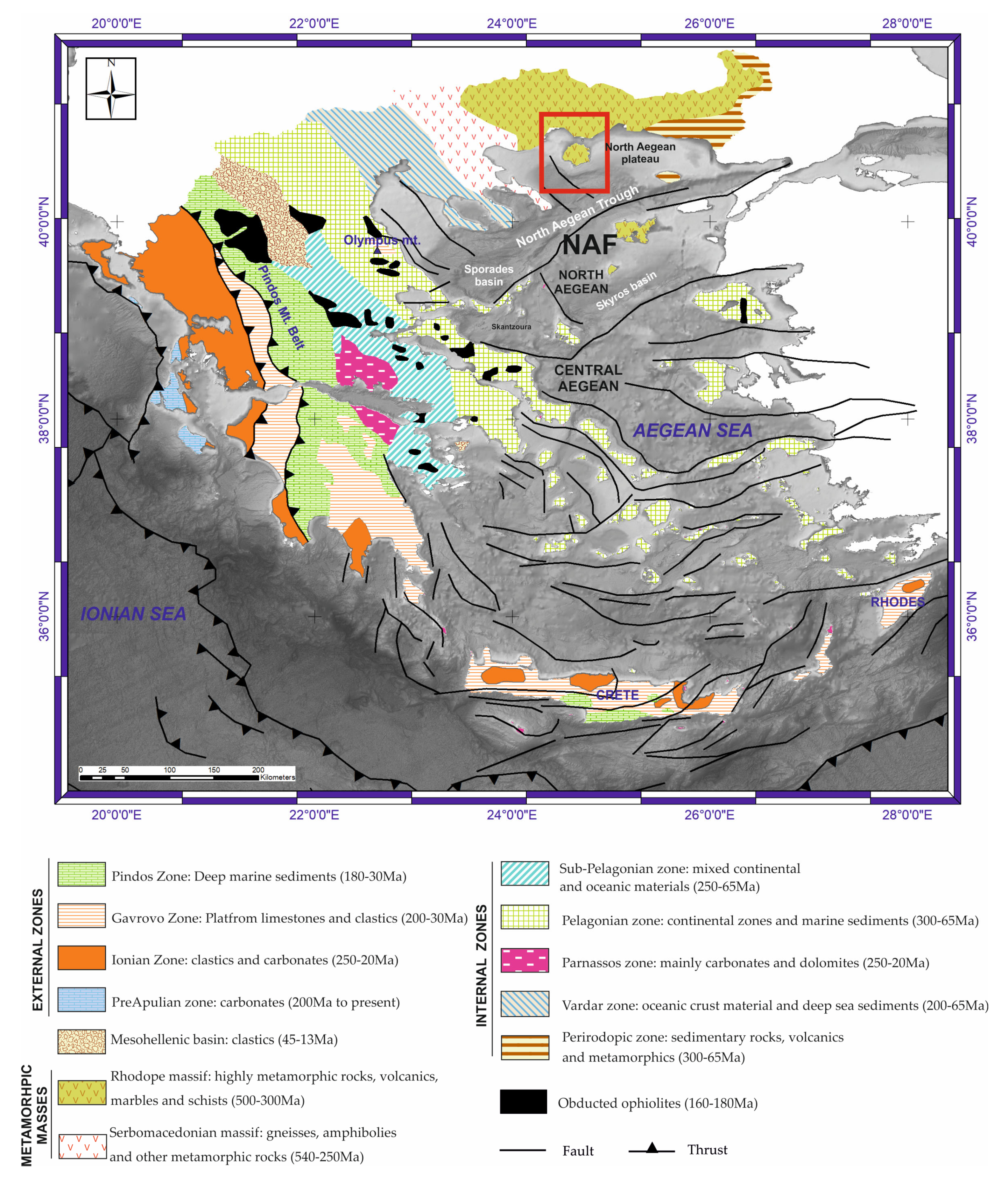
The North Aegean basins form a series of Neogene–Quaternary extensional depocenters located in northern Greece and western Turkey, extending eastwards into the Sea of Marmara [11,12]. They represent the western continuation of the North Anatolian fault zone (NAFZ) deformation system, and their evolution is closely linked to the interaction between the Aegean microplate, the Hellenic subduction zone, and westward extrusion of Anatolia [13,14] (Figure 1).
The basins display a general E–W to NE–SW orientation and are bounded by major high-angle normal and strike-slip faults. Syn-rift subsidence during the Miocene and Pliocene led to the deposition of thick sedimentary successions, locally exceeding 6 km [15]. Their stratigraphy typically includes: (a) pre-rift basement composed of metamorphic and ophiolitic complexes, belonging to the Serbomacedonian and Rhodope massifs (Figure 1) and consisting of metamorphic and highly metamorphic rocks and volcanics [11]; (b) lower–middle Miocene syn-rift marine clastics; (c) upper Miocene evaporitic deposits, particularly thick in the Prinos–Kavala Basin; and (d) Pliocene–Quaternary post-rift marine and continental clastics [11,14].
Among the North Aegean depocenters, the Prinos–Kavala Basin and the South Kavala gas field were the only ones producing oil and gas fields in Greece [15,16]. Hydrocarbon generation is associated with organic-rich Miocene shales deposited under anoxic conditions, while trapping mechanisms include fault-bounded rollover anticlines and stratigraphic pinch-outs, sealed by Messinian evaporites and shales [17].
Figure 1. Reference map of Greece showing the geotectonic zones, the major tectonic features, North Aegean basins and the study area (red rectangle). The bathymetry hillshade is from the EMODNET database [18]. NAF: North Anatolina fault. External zones *: Pindos Zone: Deep marine sediments (180-30Ma); Gavrovo Zone: Platform limestones and clastics (200-30Ma); Ionian Zone: clastics and carbonates (250-20Ma); PreApulian zone: carbonates (200Ma to present); Mesohellenic basin: clastics (45-13Ma); Internal zones *: Sub-Pelagonian zone: mixed continental and oceanic materials (250-65Ma); Pelagonian zone: continental zones and marine sediments (300-65Ma); Parnassos zone: mainly carbonates and dolomites (250-20Ma); Vardar zone: oceanic crust material and deep sea sediments (200-65Ma); Perirodopic zone: sedimentary rocks, volcanics and metamorphics (300-65Ma); Metamorhic masses: Serbomacedonian massif: gneisses, amphibolies and other metamorphic rocks (540-250Ma); Rhodope massif: highly metamorphic rocks, volcanics, marbles and schists (500-300Ma) [19]. * External zones have undergone the Tertiary orogenetic phase, while internal zones have additionally undergone the Late Mesozoic orogenetic phase.
Jmse 14 00421 g001
The evolution of the North Aegean basins is thus a product of Miocene–Recent back-arc extension, superimposed on the Hellenic subduction regime and subsequently modified by strike-slip tectonics linked to the westward propagation of the NAF. This interplay of extensional and strike-slip processes has controlled both basin morphology and sedimentary fill, shaping the petroleum system potential of the region.
The Prinos–Kavala Basin is located in the northern Aegean Sea, between the island of Thasos and the mainland of Kavala, and represents one of the most important Neogene basins of Greece [16,17,18,19]. It is an elongated NE–SW trending extensional basin, approximately 30 km in length and 15–20 km in width, that developed in response to Miocene–Pliocene taphrogenic processes. The basin is bounded by high-angle normal faults and is filled with up to 5 km of Neogene to Quaternary sediments.
The stratigraphic succession of the basin is subdivided into three main depositional intervals (Figure 2): (a) the pre-evaporitic Miocene deposits, dominated by marine clastics and shales with intercalated sandstones of turbiditic origin; (b) the Messinian evaporites, consisting mainly of anhydrites, dolomites, and halite, which form an effective regional seal; and (c) the post-evaporitic Pliocene–Pleistocene clastics, comprising marls, clays, sandstones, and conglomerates [17,20]. The reservoir units are primarily fine- to medium-grained sandstones with local microconglomerates, deposited in slope to basin-floor settings, while organic-rich shales of Miocene age represent the main hydrocarbon source rocks [21].
Structurally, the basin is characterized by fault-bounded rollover anticlines and tilted blocks. Hydrocarbon accumulations, including the Prinos oil field and the South Kavala gas field, are primarily trapped within low-relief anticlines and fault-bounded structures, with evaporitic and shale intervals acting as seals [16]. The combination of synsedimentary faulting, rapid subsidence, and evaporitic sealing conditions has played a critical role in the generation, migration, and trapping of hydrocarbons.

2.2. Reservoir Architecture

The Prinos field [21,22] consists of three main reservoirs—A, B, and C—composed of multi-layered Miocene turbiditic sandstones interbedded with shale units. These reservoirs exhibit porosities ranging from 10% to 22% and permeabilities from 2 to 2000 mD, with net-to-gross ratios between 69% and 76%. The sandstone layers are compartmentalized by faults and sealed by thick evaporites, creating overpressured (geopressured) conditions in several zones. Reservoir A, subdivided into seven layers including A1 and A2 shale intervals, contains approximately 83% of the stock-tank oil initially in place (STOIIP) and has historically produced the majority of the oil. Reservoirs B and C occur below A and remain under minimal development. The cumulative STOIIP for the Prinos base case is estimated at 291.36 MMbbl, with Reservoir A contributing the largest share, followed by Reservoir B (23.43 MMbbl) and Reservoir C (18.89 MMbbl). Bulk rock volumes reach 590.63 MMm3 across all layers.
The reservoirs are characterized by turbiditic facies ranging from coarse to fine-grained sandstones, often poorly sorted and interbedded with shales of 1 to 30 m thickness. Reservoir quality deteriorates toward the southeastern part of the field, where facies D and E dominate, consisting of thin turbiditic sandstones and argillaceous intervals with low permeability. The average net pay thickness is 97 m for Reservoir A, 22 m for Reservoir B, and 23 m for Reservoir C, with equivalent average porosities of 18%, 14.5%, and 15%, respectively. Structural complexity and fault compartmentalization influence fluid flow and make thermal and pressure management critical for both hydrocarbon recovery and CO2 injection strategies [23].

3. Materials and Methods

A total of 66 wells were analyzed across the Prinos field and some adjacent wells. The data from the wells included bottomhole temperature (BHT) logs, stratigraphic columns, pressure measurements (RFT, DST), and production records. RFT is a wireline formation testing tool used to measure formation pressure at specific depths while drilling or after drilling, before the well is completed. DST is a well test performed using drill pipe to evaluate the dynamic behavior of a reservoir interval. Seismic profiles and geological maps refined the structural interpretation. The static reservoir model, provided by Energean Oil & Gas, Kifissias Avenue, 15125 Marousi, Greece, the field operator, has been developed in Petrel 2024.8 academic license and incorporated a full 3D geological framework based on seismic interpretation and well data, detailed lithological and stratigraphic layering, and key petrophysical properties such as porosity and permeability. This model served as the foundation for subsequent thermal distribution and gradient calculations. Additionally, the well data were used to obtain wellhead temperature estimates using Ramey’s method and apply sensitivity analysis on the obtained results to cope with uncertainty.

3.1. Formation Temperature

Accurate determination of formation temperatures is essential for geothermal resource assessment. Raw BHT measurements, taken prior to setting the well in operation,—are typically lower than true formation temperatures due to the cooling effect of drilling fluids and the limited time available for thermal equilibration after that—drilling operations cease. To correct this bias, all BHT data were adjusted using the Horner method. The Horner method was adopted because the temperature data are derived from historical well reports, for which the necessary shut-in information is available. Alternative methods require more detailed drilling and circulation data that are not consistently documented for these wells.
Horner’s method, originally setup in the well test context to model pressure build up when the well was shut in, but later extended to the real bottom hole temperature estimation problem following the work of [24,25] involves plotting measured BHT values against the logarithm of the Horner time function [26] defined as:
Horner   Time   Function = t circulation + t shut - in t shut - in
where   t circulation is the duration of mud circulation and t shut - in is the elapsed time since circulation stopped. By extrapolating the linear trend of these data to infinite shut-in time (where the Horner time converges to one), the true formation temperature can be estimated. For each well, at least three BHT measurements at different shut-in times were used to construct the Horner plot, ensuring robust extrapolation and minimizing uncertainty, typically within ±8 °C [27].
With the corrected formation temperatures, the geothermal gradient for each well was calculated as the slope of the temperature–depth relationship:
Geothermal   Gradient = Δ T Δ D
where ΔT is the difference between the corrected formation temperature and the mean surface temperature (17.9 °C), and ΔD is the depth interval. Linear regression was applied to corrected temperature–depth data for each well, and gradients were mapped across the basin to identify spatial variations and thermal anomalies.

3.2. Estimation of Production Wellhead Temperature

Wellhead temperature is a key parameter for practical purposes since it reflects the heat supply of the aquifer arriving at surface. Calculating the wellhead temperature is essential to determine how hot the geothermal water will be at the surface and whether it is suitable for heating CO2 prior to injection. The wellhead temperature for the analyzed oil production well was estimated using the classical analytical approach proposed by Ramey (1962) [28], which provides a closed-form solution for transient heat transmission in flowing wells.
The method assumes single-phase fluid flow, radial heat conduction into an infinite formation, and a uniform overall heat-transfer coefficient along the wellbore. An important advantage of this approach is that it accounts for production time through the Ramey time function, allowing transient thermal effects to be captured. In contrast, some commercial software packages neglect time-dependent behavior and assume steady-state thermal conditions. Ramey’s approach balances nicely between capturing the temperature transience while neglecting few well design and fluid parameters such as the detailed trajectory and the Joule Thompson effect. Consequently, the Ramey formulation enables a more realistic representation of heat exchange along the wellbore while remaining computationally efficient.
Since detailed distributed temperature data were not available for all wells, the Ramey method was selected as an efficient and physically defensible way to approximate the temperature evolution along the well column. The method was applied to a single well, for which sufficient data were available, including a bottomhole temperature corrected using the Horner method and the necessary operational and geological parameters required to evaluate the Ramey equations.
The temperature of the produced fluid at any depth is obtained by solving the differential energy balance for a vertical conduit subjected to conductive heat losses to the surrounding formation. Ramey introduced a transient time function, f ( t ) , which accounts for the progressive development of the radial temperature disturbance in the formation:
f ( t ) = 1 2 l n ( 4 α t r p 2 ) 0.29 ,  
where α is the thermal diffusivity of the formation, t is the production time, and r p is the inner radius of the production tubing [28]. The temperature decline along the wellbore is computed using [28]:
T ( z + Δ z ) = T s ( z ) + [ T ( z ) T s ( z ) ] e x p ( Δ z X ) ,  
with T s ( z ) representing the undisturbed formation temperature at depth z , and
X = q ρ f c p [ 1 + r p U f ( t ) ] 2 π r p U ,
where q is the volumetric flow rate, ρ f and c p are the density and specific heat capacity of the geothermal fluid, and U is the overall heat-transfer coefficient [28]. Further information about the Ramey functions can be found in Appendix A, Appendix B and Appendix C. Between the flowing fluid and the formation, accounting for the insulation effect of the equipment (i.e., tubing, annulus brine, casing and cement). To generate the temperature profiles Equation (4) needs to be integrated iteratively from bottom hole depth up to the wellhead.
For the analyzed production well, the governing equations of the Ramey analytical method were evaluated numerically along the depth using a stepwise vertical discretization of the wellbore. A customized computational script was developed to automate the temperature-marching calculation, starting from the Horner-corrected bottomhole temperature and progressing upward to the wellhead. The script computes the Ramey time function, the depth-dependent formation temperature based on the geothermal gradient derived for this well, the characteristic length X, and the incremental temperature decay for each depth step. The wellhead temperature is determined from the final near-surface interval.
Because detailed data allowing for the full application of the Ramey method were only available for a single well, the calculation relied on site-specific parameters including the corrected bottomhole temperature, measured flow rate, tubing geometry, and the geothermal gradient obtained from the Horner analysis. Fluid thermophysical properties were taken from standard correlations, while formation thermal diffusivity and overall heat-transfer coefficients were selected from published ranges appropriate for similar geothermal and petroleum reservoirs. The values utilized in this work are shown in the Results Section 4.

3.3. Reservoir Pressure Conditions

Pressure–depth data from RFT and DST were analyzed to identify subsurface pressure conditions. Measured pressures were plotted against depth and compared to theoretical hydrostatic and lithostatic gradients. This approach allowed identification of zones with pressure anomalies and assessment of their relationship to structural and stratigraphic features. Geological evidence, including thick Messinian evaporite seals and fault compartmentalization, was also considered, as these features influence fluid migration and pressure distribution within the basin.

4. Results

4.1. Calculation of Geothermal Gradient Using Corrected BHT

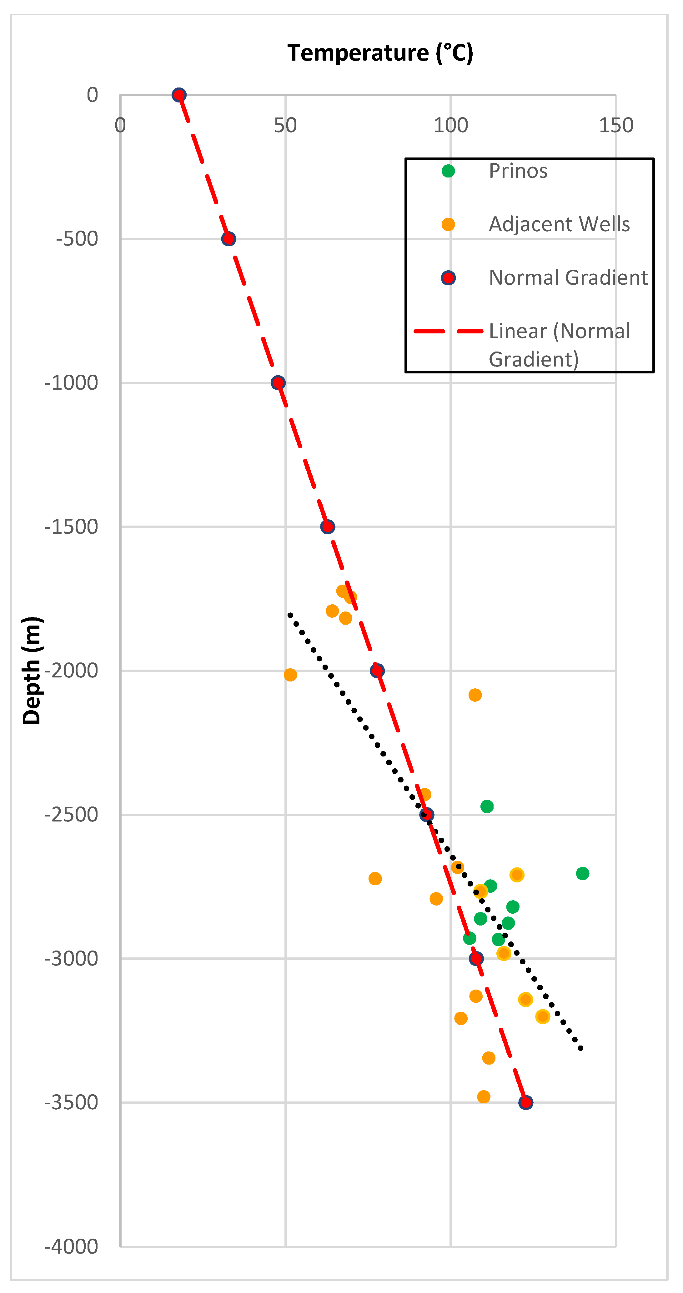
Corrected BHT data reveal significant spatial variability in geothermal gradients across the basin. The average geothermal gradient is approximately 30 °C/km (Figure 3), with local anomalies exceeding 40 °C/km in structurally favorable zones. Isothermal mapping identifies areas where temperatures exceed 90 °C at depths suitable for direct use and power generation.
To further assess the geothermal potential, the depth to the 90 °C isotherm was mapped throughout the basin. The 90 °C isotherm (Figure 4) is a critical threshold for medium enthalpy geothermal systems [29] marking the minimum temperature suitable for efficient direct heating and binary cycle power generation. Using the corrected temperature data and geothermal gradients, temperature–depth profiles were interpolated, using standard geostatistical tools (kriging method) and isothermal surfaces were generated using Petrel software 2024.8 academic license. The resulting maps highlight zones where the 90 °C isotherm is shallow, indicating the most accessible and productive geothermal targets. Areas where the 90 °C isotherm occurs at economically drillable depths (e.g., less than 3000 m) were prioritized for development.

4.2. Wellhead Temperature

To calculate the wellhead temperature using Ramey’s method, a single well was selected, for which the bottomhole temperature was corrected using the Horner method, and operational data were available. The following parameters refer to this well. The input parameters used in the application of the Ramey method are presented in Table 1.
The heat transfer coefficient values were based on the work of Kedzierski et al. (2016) [30].
Wellbore depth and geometric dimensions were obtained from well reports provided by Energean, including tubing dimensions, pipe inner radius, and measured surface formation temperature. The bottomhole temperature, 117.41 °C was estimated from the available downhole data and subsequently corrected using the Horner method.
To apply Ramey’s method, a vertical step size of 10 m was adopted to ensure fine resolution of the temperature profile while maintaining computational efficiency, whereas a fluid density of 1020 kg/m3 was adopted to represent saline formation water, consistent with values reported for deep sedimentary reservoir brines in geothermal and petroleum systems [31].
A specific heat capacity of 3700 J/kg/K was selected to represent saline, water-dominated formation fluids, in agreement with commonly used thermophysical properties in geothermal and wellbore heat-transfer analyses [32].
The formation thermal diffusivity was assumed equal to 1.0 × 10⁻⁶ m2/s, which lies within the typical range reported for sedimentary and fractured rock formations and is frequently employed in analytical wellbore heat-transfer models when site-specific measurements are unavailable [33,34].
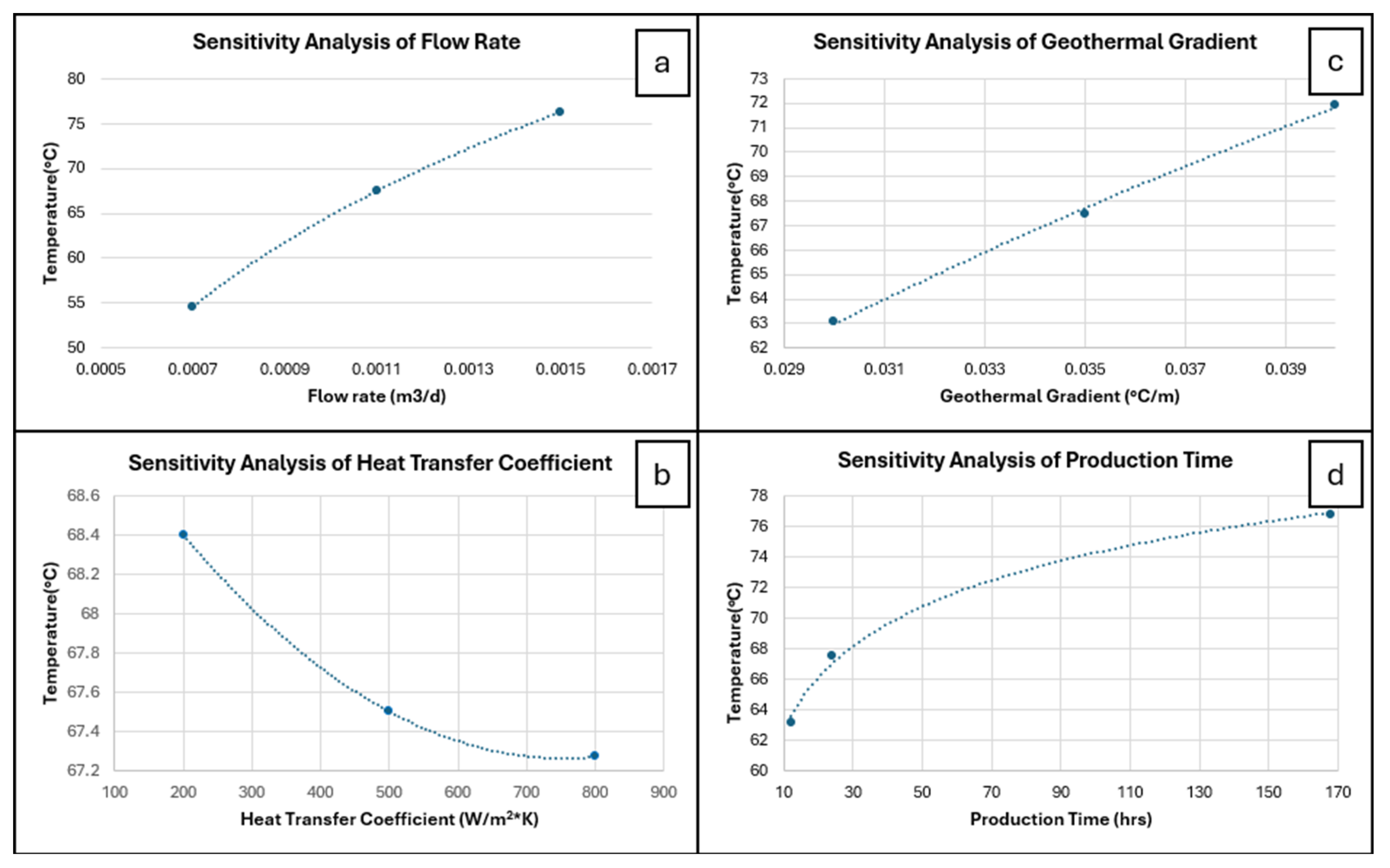
Once the wellhead temperature calculations were completed, a sensitivity analysis was conducted (see Figure 5) to evaluate the influence of key operational and thermal parameters on the estimated wellhead temperature obtained from the Ramey analytical model. The analysis focused on four primary variables: produced water flow rate, overall heat-transfer coefficient, geothermal gradient and production rates. For each parameter, base, maximum, and minimum scenarios were examined while constantly maintaining the well geometry and the fluid properties. The bullets represent three different scenarios. The bullet in the middle of each plot represents the base case scenario.
Although only three points are shown, the analysis was not based solely on them. Insights from Ramey’s equations informed the functional form imposed on the curve-fitting algorithm, effectively incorporating additional information. A dense grid of additional points confirmed that the data followed the same trendline, validating the chosen functional forms and supporting the robustness of the analysis.
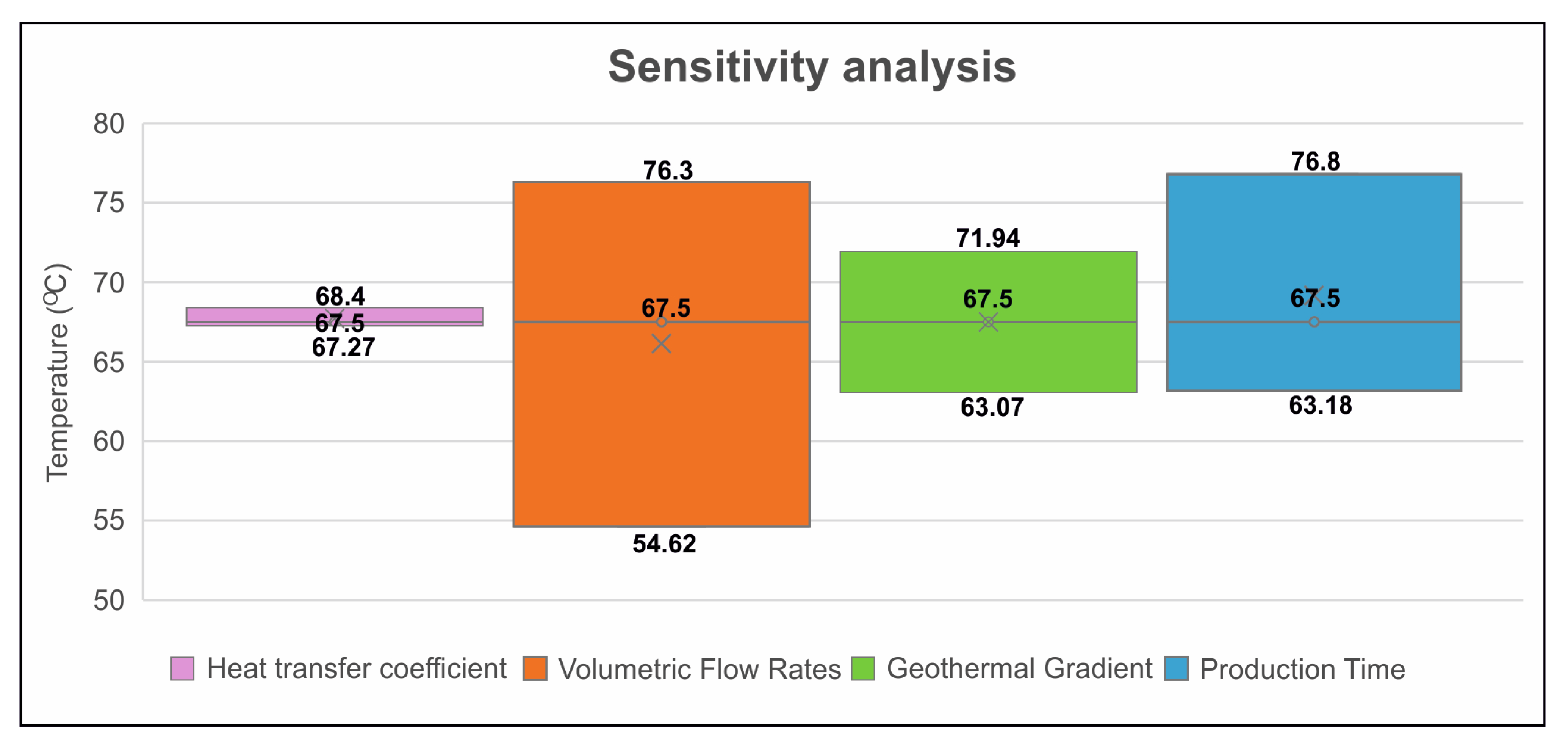
The first sensitivity scenario evaluated the effect of produced water flow rate. Based on available field reports, a base flow rate of approximately 100 m3/day was selected, with minimum and maximum values of 63 m3/day and 136 m3/day, respectively. Figure 5a suggests that a strong positive correlation between flow rate (x-axis, in m3/day) and temperature (y-axis, in °C). As flow rate increases from approximately 63 m3/day to 136 m3/day, the predicted wellhead temperature rises from about 55 °C to nearly 75 °C. This behavior indicates that flow rate exerts a strong influence on the predicted wellhead temperature. Lower flow rates than 63 m3/day result in increased residence time of the fluid within the wellbore, thereby enhancing conductive heat losses to the surrounding formation and leading to a substantial reduction in wellhead temperature. Conversely, higher flow rates preserve more of the bottomhole thermal energy due to dominant advective heat transport, yielding higher wellhead temperatures. This behavior is a result of the theoretical structure of the Ramey solution, wherein the characteristic thermal decay length is directly proportional to the product of flow rate, fluid density, and specific heat capacity, and inversely related to the effective heat exchange with the formation.
The second sensitivity scenario examined the impact of the overall heat-transfer coefficient. A base value of 500 W/m2*K was adopted, with minimum and maximum values of 200 and 800 W/m2*K, respectively. According to Figure 5b there is a negative correlation between U (x-axis, in W/m2*K) and temperature (y-axis, in °C). As U increases from 200 to 800 W/m2*K, the predicted wellhead temperature decreases marginally from approximately 68.4 °C to 67.27 °C. This trend indicates that while heat-transfer coefficient influences thermal behavior, its effect is minor. Increasing the heat-transfer coefficient enhanced thermal communication between the flowing fluid and the formation, resulting in greater temperature attenuation along the wellbore. However, compared to flow rate variations, changes in the overall heat-transfer coefficient produced a more moderate effect on the final wellhead temperature. This indicates that, under the analyzed conditions, convective heat transport within the well dominates over conductive losses to the formation. Unlike simpler approaches, which limit conduction effects to steady state (assuming that the formation temperature profile with depth does not vary over time), Ramey’s method assumes that sooner or later—as dictated by the heat-transfer coefficient—the temperature profile, and hence the wellhead temperature, will converge to a fixed value. In other words, if infinite flow time were allowed, the wellhead temperature would not depend on the heat-transfer coefficient.
The third scenario assessed sensitivity to the geothermal gradient, with a base value of 0.035 °C/m and bounds of 0.03 °C/m and 0.04 °C/m. Figure 5c shows that increasing the gradient from 0.03 °C/m to 0.04 °C/m raises the predicted wellhead temperature from about 63.07 °C to 71.94 °C. Variations in geothermal gradient directly affected the formation temperature profile and, consequently, the thermal driving force between the wellbore fluid and the surrounding rock. Higher geothermal gradients resulted in higher wellhead temperatures due to elevated formation temperatures along the well depth, while lower gradients increased thermal losses. Although the geothermal gradient influenced the absolute temperature levels, its effect remained secondary to that of flow rate.
Finally, production times were analyzed using three scenarios: 12 h, 24 h and 1 week. The temperature values at the wellhead showed an increasing trend reaching at the 1-week scenario a value of 76.8 °C. This is the effect of the thermal stabilization of the wellbore. As production continues, heat is transferred from the flowing fluid to the surrounding formations, gradually warming the near-wellbore region. As a result, the effective geothermal gradient experienced by the fluid during upward flow becomes smaller, leading to less heat diffusion from the fluid to the formation and higher fluid temperatures at the surface.
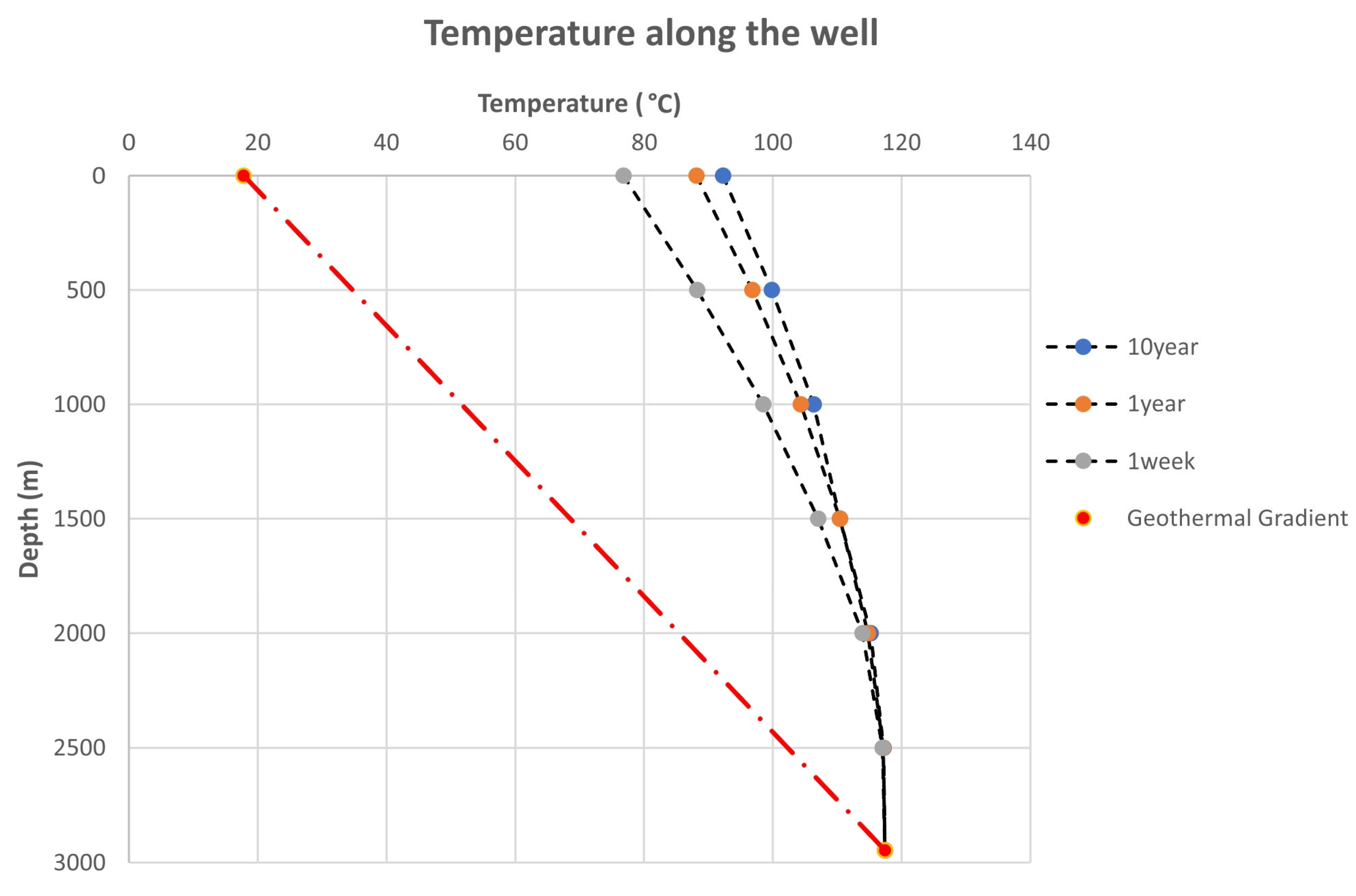
According to Ramey (1962) [28], who showed that wellbore temperatures increase with time as the earth surrounding the wellbore becomes heated, and that temperature changes may continue slowly even over very long periods due to the low thermal diffusivity of geological formations. In the present case (see Figure 6), the same physical mechanism explains why longer production times lead to higher wellhead temperatures and a temperature profile that moves closer to the normal geothermal gradient with time.

4.3. Pressure Distribution

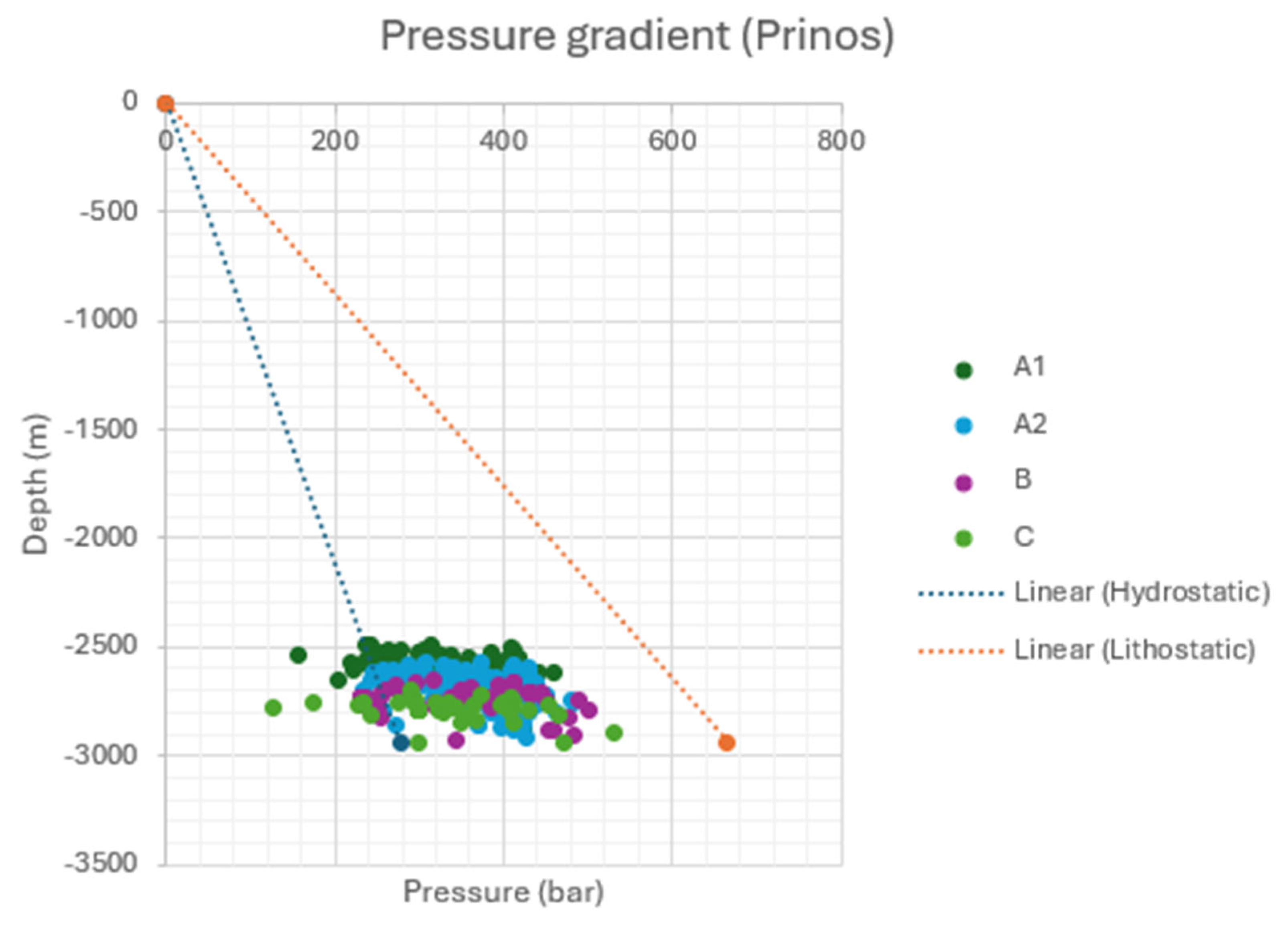
The analysis of pressure–depth data from RFT and DST logs revealed the presence of geopressured reservoirs in the Miocene turbiditic sandstones of the Prinos field. Measured pressures in these zones consistently exceeded the theoretical hydrostatic gradient and, in some cases, approached the lithostatic gradient, confirming the existence of overpressured (geopressured) conditions (Figure 7). These conditions are primarily the result of rapid sedimentation, the presence of low-permeability Messinian evaporite seals, and limited fluid escape pathways. Fault compartmentalization further enhances pressure heterogeneity within the reservoirs, creating distinct pressure compartments that must be carefully managed during exploitation.
The identification of geopressured zones is significant for both geothermal and hydrocarbon exploitation. Geopressured reservoirs offer higher enthalpy and fluid flow rates, which are advantageous for geothermal energy production, but they also present operational challenges related to well control, casing integrity, and reservoir management. The recognition of these zones in the Prinos–Kavala Basin underscores the need for tailored drilling and production strategies to ensure safe and efficient resource development.

5. Discussion

The corrected BHT data and subsequent geothermal gradient mapping provided the basis for assessing the thermal regime of the Prinos–Kavala Basin. The application of the Horner method reduced the uncertainty in formation temperature estimates, enabling the interpolation of temperature–depth profiles and the identification of zones where the 90 °C isotherm occurs at drillable depths. These areas represent prime targets for medium-enthalpy geothermal exploitation, supporting direct-use applications and binary-cycle power generation.
Beyond the static thermal characterization, the dynamic performance was evaluated using the Ramey analytical model, which accounts for transient heat transfer during fluid ascent in the wellbore. This approach allowed the estimation of wellhead temperatures under varying operational conditions, bridging the gap between formation temperature and deliverable energy at the surface. The Ramey calculations confirmed that the advective heat transport dominates over conductive losses under typical production scenarios, emphasizing the importance of flow-rate management in preserving thermal energy.
The sensitivity analysis presented in the previous sections demonstrated that the flow rate is the most critical control, with higher rates significantly reducing residence time and conductive losses, thereby increasing the wellhead temperature up to 20 °C across the tested range (Figure 8). A fact that also delineates the effect of flow rate in wellbore temperature is that according to provided data by the operator (Energean Oil and Gas) the wellbore temperatures at the various wells vary from 30 °C to 100 °C. These variations cannot be attributed to the physical heterogeneities of the system considering the limited spatial extend of the analyzed oil field. It is also possible that these variations could be attributed to the effect of cold gas lift used to produce fluids. Unfortunately, accurate flow rate records are not available for many of the wells. Variations in the heat-transfer coefficient produced only minor temperature changes (~1–2 °C), indicating that wall/formation exchange plays a secondary role when the convective transport is strong. The geothermal gradient exerted a moderate effect, with higher gradients enhancing the baseline temperatures but remaining less influential than the flow rate. These findings align with the theoretical structure of the Ramey solution, where the characteristic thermal decay length is strongly dependent on mass flow and fluid properties. The sensitivity analysis did not include other parameters, for example the pipeline diameter since Prinos is a depleted oil field with the existing wells, which will be probably used for the planned CCS project.
In any case, the extraction of warm brine from the reservoir represents a valuable asset for potential CCS projects, depending on the injection strategy adopted. There is an ongoing debate regarding whether CO2 should be injected under supercritical conditions or in liquid form [35]. Liquid CO2 offers the advantage of higher density, thereby requiring lower compression energy for injection into the reservoir [35]. However, liquid CO2 is typically significantly cooler than in situ reservoir conditions, which may induce thermal contraction effects, potentially damage the wellbore casing or cause radial cracking in the cement sheath used for well stabilization [36,37]. To mitigate these risks, preheating of the injected CO2 has been implemented with positive outcomes in both field applications [38] and numerical simulation studies [39]. In particular, for offshore CCS projects—where access to external heat sources is limited—the exploitation of medium-enthalpy geothermal resources may provide a cost-effective solution. In this context, production wells used to manage the CO2 plume could serve a dual purpose by also supplying warm brine for CO2 preheating.
The integration of corrected BHT data, geothermal mapping, and Ramey-based sensitivity analysis provides a comprehensive framework for resource evaluation. From a practical standpoint, the rate optimization emerges as the primary operational level for maximizing recoverable thermal energy, while site selection should prioritize zones with favorable geothermal gradients and manageable drilling depths. The identification of geopressured reservoirs further enhances the potential for high-enthalpy production but introduces operational challenges that require tailored well design and pressure management strategies. Additionally, once the well begins operating, the wellhead temperature will be measured, allowing the model to be calibrated against these actual observations.
Future work will focus on expanding the current analysis to all available production wells. Bottomhole temperatures have now been estimated for the entire well set, and geothermal gradients have been determined for the wells where adequate shut-in information was available. The next step is to develop a practical optimization framework that can make use of these data to identify which wells are best suited for supplying the hot water needed for CO2 heating at the surface. This may involve applying algorithmic or data-driven methods to evaluate different flow-rate scenarios and to determine how production should be distributed among the wells to achieve the required temperature levels. Once these approaches are tested, they can form the basis for a field-scale strategy that links geothermal heat availability to CO2 handling and surface-facility operation.

6. Conclusions

This study provides a comprehensive evaluation of the geothermal potential of the Prinos–Kavala Basin through integrated thermal correction, dynamic and sensitivity analysis. The application of the Horner method to BHT data significantly improved the accuracy of formation temperature estimates, enabling reliable geothermal gradient mapping and identification of zones where the 90 °C isotherm occurs at economically drillable depths. The analysis of the corrected temperature data and their demonstration with typical geothermal gradient showed that the Prinos reservoir has significantly higher temperatures than those expected from a typical geothermal gradient, confirming an elevated thermal gradient in the area. Notably, the isotherm mapping highlights that the reservoir zones have clear geothermal development potential, because they exceed the 90 °C threshold, which is the lower limit for medium-enthalpy geothermal systems. These zones are suitable for direct-use heating applications and binary-cycle power generation.
Dynamic analysis using the Ramey analytical model bridged the gap between static formation temperatures and deliverable wellhead conditions, confirming that advective heat transport dominates thermal behavior during production. The sensitivity analysis further demonstrated that flow rate is the most influential operational parameter, exerting a far greater impact on wellhead temperature than variations in heat-transfer coefficient or geothermal gradient. These findings underscore the importance of flow-rate optimization in maximizing thermal energy recovery. Additionally, the results from the Ramey analytical method showed that the expected wellhead temperatures range between 54.6 °C and 76.8 °C. These temperatures are high enough to allow preheating of CO2 before injection, showing a link between geothermal heat extraction and CO2 storage operations.
The identification of geopressured reservoirs within Miocene turbiditic sandstones adds an additional dimension to resource potential, offering higher enthalpy and fluid flow rates but requiring tailored well design and pressure management strategies. Collectively, these insights highlight the value of a multidisciplinary approach—combining corrected thermal data, dynamic modeling, and parametric sensitivity—to guide exploration and development in structurally complex basins.
In conclusion, these results demonstrate that the Prinos–Kavala Basin has strong geothermal potential, supported by high subsurface temperatures, favorable wellhead conditions, and geological features conducive to sustainable heat extraction. This work underscores the importance of a multidisciplinary workflow—combining corrected temperature data, dynamic, and sensitivity analysis—to guide geothermal evaluation in structurally complex basins.
Future work should focus on integrating these findings into advanced reservoir simulation and techno-economic assessments to optimize well placement, production strategies, and the potential coupling of geothermal energy with CO2 storage. Such efforts will ensure safe, efficient, and sustainable utilization of the region’s geothermal resources.

Author Contributions

Conceptualization, A.R. and I.V.; methodology, A.R. and I.V.; validation, A.R. and I.V.; writing—original draft preparation, A.R. and I.V.; review and editing I.V., P.K., Y.T., G.A., F.P. and V.G. All authors have read and agreed to the published version of the manuscript.

Funding

This research received no external funding.

Data Availability Statement

All data used are presented in the manuscript.

Acknowledgments

The authors gratefully acknowledge Energean Oil & Gas for providing the dataset used to conduct this analysis. Additionally, Adamantia Raftogianni would like to thank the Special Account for Research Funding (E.L.K.E.) of the National Technical University of Athens (N.T.U.A.) for supporting her Ph.D. studies through a scholarship.

Conflicts of Interest

Authors Paschalia Kiomourtzi and Yannis Tsiantis were employed by the company Energean Oil & Gas. The remaining authors declare that the research was conducted in the absence of any commercial or financial relationships that could be construed as a potential conflict of interest.

Appendix A. Ramey Time Function

Ramey [28] introduced a transient time function, f ( t ) , to account for radial heat conduction from the wellbore into the surrounding formation. The time function is expressed as
f ( t ) = l n ( r p 2 α t ) 0.29 ,
where α is the thermal diffusivity of the formation, t is the production time, and r p is the inner radius of the pipe. This expression can be equivalently written as
ln ( r p 2 α t ) = ln ( 2 α t r p ) = ln ( ( 4 α t r p 2 ) 1 2 ) = 1 2 ln ( 4 α t r p 2 ) ,

Appendix B. Characteristic Length Parameter

The characteristic thermal decay length used in the present study is defined as
X = q ρ f ˙ c p [ 1 + r p U f ( t ) ] 2 π r p U ,
where m ˙ = q ρ f is the mass flow rate, q is the volumetric flow rate, ρ f is the fluid density, c p is the fluid specific heat capacity, and U is the heat-transfer coefficient. This formulation is mathematically equivalent to the characteristic length parameter A defined by Ramey [28], which incorporates formation thermal conductivity through the heat-transfer term.
In the original Ramey formulation, the formation thermal conductivity k appears explicitly in the heat-transfer relationship. In this study, a representative thermal conductivity value of 1 W·m−1·K−1 was assumed, consistent with reported ranges for sandy sedimentary formations surrounding the well [32].

Appendix C. Ramey Formulation

Ramey’s original analytical solution describes the temperature of a flowing fluid along a producing well as a function of depth and time. The solution can be expressed as
T ( z , t ) = a z + b a A + ( T 0 + a A b ) e x p ( z A ) ,
where z is the depth along the well, a is the geothermal gradient, b is the surface formation temperature, T 0 is the bottomhole fluid temperature, and A is the characteristic thermal decay length. The surrounding formation temperature at depth z is given by
T s ( z ) = a z + b .
Subtracting the formation temperature from the fluid temperature yields
T ( z ) T s ( z ) = [ T 0 T s ( 0 ) ] e x p ( z A ) ,
which demonstrates that the temperature difference between the flowing fluid and the surrounding formation decays exponentially with depth.
For numerical implementation, the continuous depth coordinate z is discretized into small vertical increments Δ z . Over a single depth interval, the exponential decay relationship can be written as
T ( z + Δ z ) T s ( z ) = [ T ( z ) T s ( z ) ] e x p ( Δ z A ) .
Rearranging this expression yields the stepwise temperature-marching equation:
T ( z + Δ z ) = T s ( z ) + [ T ( z ) T s ( z ) ] e x p ( Δ z A ) .
This discrete formulation represents a numerical implementation of Ramey’s analytical solution. As the step size Δ z becomes sufficiently small, the stepwise solution converges to the continuous analytical expression.

References

  1. Papachristou, M.; Dalampakis, P.; Arvanitis, A.; Mendrinos, D.; Andritsos, N. Geothermal developments in Greece–country update 2015–2020. In Proceedings of the World Geothermal Congress 2020+1, Reykjavik, Iceland, April–October 2021; Volume 1. Available online: https://www.researchgate.net/profile/Apostolos-Arvanitis/publication/359193522_Geothermal_Developments_in_Greece_-_Country_Update_2015-2020/links/622cb3baa39db062db971f1a/Geothermal-Developments-in-Greece-Country-Update-2015-2020.pdf (accessed on 20 October 2025).
  2. Kolios, N.; Fytikas, M.; Arvanitis, A.; Andritsos, N.; Koutsinos, S. Prospective medium enthalpy geothermal resources in sedimentary basins of Northern Greece. In Proceedings of the European Geothermal Congress, Unterhaching, Germany, 30 May–1 June 2007; Available online: https://www.researchgate.net/profile/Apostolos-Arvanitis/publication/266369107_Prospective_Medium_Enthalpy_Geothermal_Resources_in_Sedimentary_Basins_of_Northern_Greece/links/550135d50cf2de950a71d958/Prospective-Medium-Enthalpy-Geothermal-Resources-in-Sedimentary-Basins-of-Northern-Greece.pdf (accessed on 14 November 2025).
  3. Thanassoulas, C.; Lazou, A. The Nestos Delta Geothermal Field and Its Relation to the Associated Self Potential (SP) Field. Geothermics 1993, 22, 117–134. [Google Scholar] [CrossRef] [Scilit]
  4. Shaharizuan, W.; Sabdullah, N.; Aenun, S.; Bosamah, N.B. A Review of Global Carbon Capture and Storage (CCS) and Carbon Capture, Utilization, and Storage (CCUS). E3S Web Conf. 2024, 516, 01009. [Google Scholar] [CrossRef] [Scilit]
  5. Nazarian, B.; Furre, A.K. Simulation study of Sleipner plume on entire Utsira using a multi-physics modelling approach. In Proceedings of the 16th Greenhouse Gas Control Technologies Conference (GHGT-16), Lyon, France, 23–27 October 2022; pp. 23–24. [Google Scholar] [CrossRef] [Scilit]
  6. Shell Canada. Quest Carbon Capture and Storage Project Annual Report; Shell Canada Ltd.: Calgary, AB, Canada, 2016; Available online: https://open.alberta.ca/dataset/2ef6c060-69a5-4bde-9ae5-370f6b9219fc/resource/6cef6362-ac54-4911-b263-fe1aa0ee28c9/download/ccsquestreport2016.pdf (accessed on 17 September 2025).
  7. Jiang, P.; Li, X.; Xu, R.; Wang, Y.; Chen, M.; Wang, H.; Ruan, B. Thermal modeling of CO2 in the injection well and reservoir at the Ordos CCS demonstration project, China. Int. J. Greenh. Gas Control. 2014, 23, 135–146. [Google Scholar] [CrossRef] [Scilit]
  8. Tanaka, Y.; Abe, M.; Sawada, Y.; Tanase, D.; Ito, T.; Kasukawa, T. Tomakomai CCS demonstration project in Japan: 2014 update. Energy Procedia 2014, 63, 6111–6119. [Google Scholar] [CrossRef] [Scilit]
  9. Kiomourtzi, P. Prinos CO2 storage—A pioneer case study for SE Europe. In Proceedings of the Fourth EAGE Eastern Mediterranean Workshop; European Association of Geoscientists & Engineers: Bunnik, The Netherlands, 2023; Volume 2023. [Google Scholar] [CrossRef] [Scilit]
  10. Amvrazis, M.; Ismail, I.; Ktenas, D.; Gaganis, V.; Tartaras, E.; Stefatos, A. Prinos CO2 storage permit application: An integrated technical and regulatory workflow. In Proceedings of the Fifth EAGE Eastern Mediterranean Workshop; European Association of Geoscientists & Engineers: Bunnik, The Netherlands, 2025; Volume 2025, pp. 1–3. [Google Scholar] [CrossRef] [Scilit]
  11. Papanikolaou, D. The tectonostratigraphic terranes of the Hellenides. Ann. Géologiques Des Pays Helléniques 1997, 37, 495–514. [Google Scholar]
  12. Lybéris, N. Tectonic evolution of the North Aegean trough. Geol. Soc. Lond. Spec. Publ. 1984, 17, 709–725. [Google Scholar] [CrossRef] [Scilit]
  13. Mascle, J.; Martin, L. Shallow structure and recent evolution of the North Aegean Sea: A synthesis based on continuous reflection profiles. Mar. Geol. 1990, 94, 271–299. [Google Scholar] [CrossRef] [Scilit]
  14. Armijo, R.; Meyer, B.; Hubert, A.; Barka, A. Westward propagation of the North Anatolian fault into the northern Aegean: Timing and kinematics. Geology 1999, 27, 267–270. [Google Scholar] [CrossRef] [Scilit]
  15. Piper, D.J.; Perissoratis, C. Late Quaternary sedimentation on the North Aegean Continental Margin, Greece. AAPG Bull. 1991, 75, 46–61. [Google Scholar] [CrossRef] [Scilit]
  16. Proedrou, P. South Kavala gas field—Taphrogenetic Prinos Basin. Bull. Geol. Soc. Greece 2001, 34, 1221–1228. [Google Scholar] [CrossRef] [Scilit]
  17. Beniest, J.P.; Brun, J.-P.; Gorini, C.; Crombez, V.; Deschamps, R.; Hamon, Y.; Smit, J. Interaction between trench retreat and Anatolian escape as recorded by Neogene basins in the northern Aegean Sea. Mar. Pet. Geol. 2016, 77, 30–42. [Google Scholar] [CrossRef] [Scilit]
  18. EMODnet Bathymetry Consortium. Emodnet Digital Bathymetry (dtm 2016). Available online: https://sextant.ifremer.fr/record/c7b53704-999d-4721-b1a3-04ec60c87238/ (accessed on 2 February 2018).
  19. Kiomourtzi, P.; Pasadakis, N.; Zelilidis, A. Geochemical characterization of satellite hydrocarbon formations in the Prinos–Kavala Basin. Bull. Geol. Soc. Greece 2007, 40, 394–405. [Google Scholar] [CrossRef] [Scilit]
  20. Mertzanides, Y.; Kargiotis, E.; Mitropoulos, A. Geological and geophysical data of “Epsilon” field in Prinos oil basin. Bull. Geol. Soc. Greece 2010, 43, 2257–2264. [Google Scholar] [CrossRef] [Scilit]
  21. Kiomourtzi, P. Depositional Environments and Hydrocarbon Potential Basins in the North Aegean Sea. Ph.D. Thesis, University of Patras, Patras, Greece, 2016. [Google Scholar]
  22. Ioakeimidis, I.; Kantiranis, N.; Georgakopoulos, A.; Kiomourtzi, P.; Tsirambides, A. Diagenetic Processes in the Reservoir of the Prinos Oil Field, Prinos–Kavala Basin, Macedonia, Greece. Available online: http://etdedata.gein.noa.gr/PROCEEDINGS_15th_CONGRESS_GSG_2019/T6-%CE%A46S1.Geo-Energy%20from%20Exploration%20to%20Technological%20Advances%20and%20Sustainability/GSG_2019_paper_148.pdf (accessed on 6 November 2025).
  23. Proedrou, P.; Sidiropoulos, T. Prinos Field—Greece Aegean Basin; Public Petroleum Corporation of Greece: Athens, Greece, 2004; Available online: https://archives.datapages.com/data/specpubs/fieldst3/data/a020/a020/0001/0250/0275.htm#purchaseoptions (accessed on 2 October 2025).
  24. Fertl, W.H. Abnormal Formation Pressures, 1st ed.; Elsevier: Amsterdam, The Netherlands, 1981; Volume 2. [Google Scholar]
  25. Dowdle, W.L.; Cobb, W.M. Static Formation Temperature From Well Logs—An Empirical Method. J. Pet. Technol. 1975, 27, 1326–1330. [Google Scholar] [CrossRef] [Scilit]
  26. Horner, R.D. Pressure build-up in wells. In Proceedings of the Third World Petroleum Congress, The Hague, The Netherlands, 28 May–6 June 1951; Brill: Leiden, The Netherlands, 1951; Volume 34, p. 316. [Google Scholar]
  27. Available online: https://www.zetaware.com/utilities/bht/horner.html (accessed on 2 October 2025).
  28. Ramey, H.J., Jr. Wellbore heat transmission. J. Pet. Technol. 1962, 14, 427. [Google Scholar] [CrossRef] [Scilit]
  29. Dickson, M.H.; Fanelli, M. Small Geothermal Resources: A Review. Energy Sources 1994, 16, 349–376. [Google Scholar] [CrossRef] [Scilit]
  30. Kędzierski, P.; Nagórski, Z.; Niezgoda, T. Determination of local values of heat transfer coefficient in geothermal models with internal functions method. Renew. Energy 2016, 92, 506–516. [Google Scholar] [CrossRef] [Scilit]
  31. Ito, M.; Azam, S. Feasibility of saline gradient solar ponds as thermal energy sources in Saskatchewan, Canada. J. Environ. Inform. Lett. 2019, 1, 72–80. [Google Scholar] [CrossRef] [Scilit]
  32. Available online: https://geomodel.pl/en/thermophysical-parameters-of-brines/ (accessed on 7 November 2025).
  33. Fuchs, S.; Förster, H.J.; Norden, B.; Balling, N.; Miele, R.; Heckenbach, E.; Förster, A. The thermal diffusivity of sedimentary rocks: Empirical validation of a physically based α−φ relation. J. Geophys. Res. Solid Earth 2021, 126, e2020JB020595. [Google Scholar] [CrossRef] [Scilit]
  34. Al Nakshabandi, G.; Kohnke, H. Thermal conductivity and diffusivity of soils as related to moisture tension and other physical properties. Agric. Meteorol. 1965, 2, 271–279. [Google Scholar] [CrossRef] [Scilit]
  35. Vilarrasa, V.; Silva, O.; Carrera, J.; Olivella, S. Liquid CO2 injection for geological storage in deep saline aquifers. Int. J. Greenh. Gas Control. 2013, 14, 84–96. [Google Scholar] [CrossRef] [Scilit]
  36. Teodoriu, C. Why and when does casing fail in geothermal wells: A surprising question? In Proceedings of the World Geothermal Congress 2015, Melbourne, Australia, 19–25 April 2015. Available online: https://www.osti.gov/etdeweb/biblio/22090676 (accessed on 14 November 2025).
  37. Roy, P.; Walsh, S.D.; Morris, J.P.; Iyer, J.; Hao, Y.; Carroll, S.; Gawell, K.; Todorovic, J.; Torsæter, M. Studying the impact of thermal cycling on wellbore integrity during CO2 injection. In Proceedings of the American Rock Mechanics Association, Houston, TX, USA, 26–29 June 2016; Paper No. 16-0668. Available online: https://onepetro.org/ARMAUSRMS/proceedings-abstract/ARMA16/All-ARMA16/126382 (accessed on 17 November 2025).
  38. Möller, F.; Liebscher, A.; Martens, S.; Schmidt-Hattenberger, C.; Streibel, M. Injection of CO2 at ambient temperature conditions—Pressure and temperature results of the “cold injection” experiment at the Ketzin pilot site. Energy Procedia 2014, 63, 6289–6297. [Google Scholar] [CrossRef] [Scilit]
  39. Nimtz, M.; Klatt, M.; Wiese, B.; Kühn, M.; Krautz, H.-J. Modelling of the CO2 process- and transport chain in CCS systems—Examination of transport and storage processes. Geochemistry 2010, 70, 185–192. [Google Scholar] [CrossRef] [Scilit]
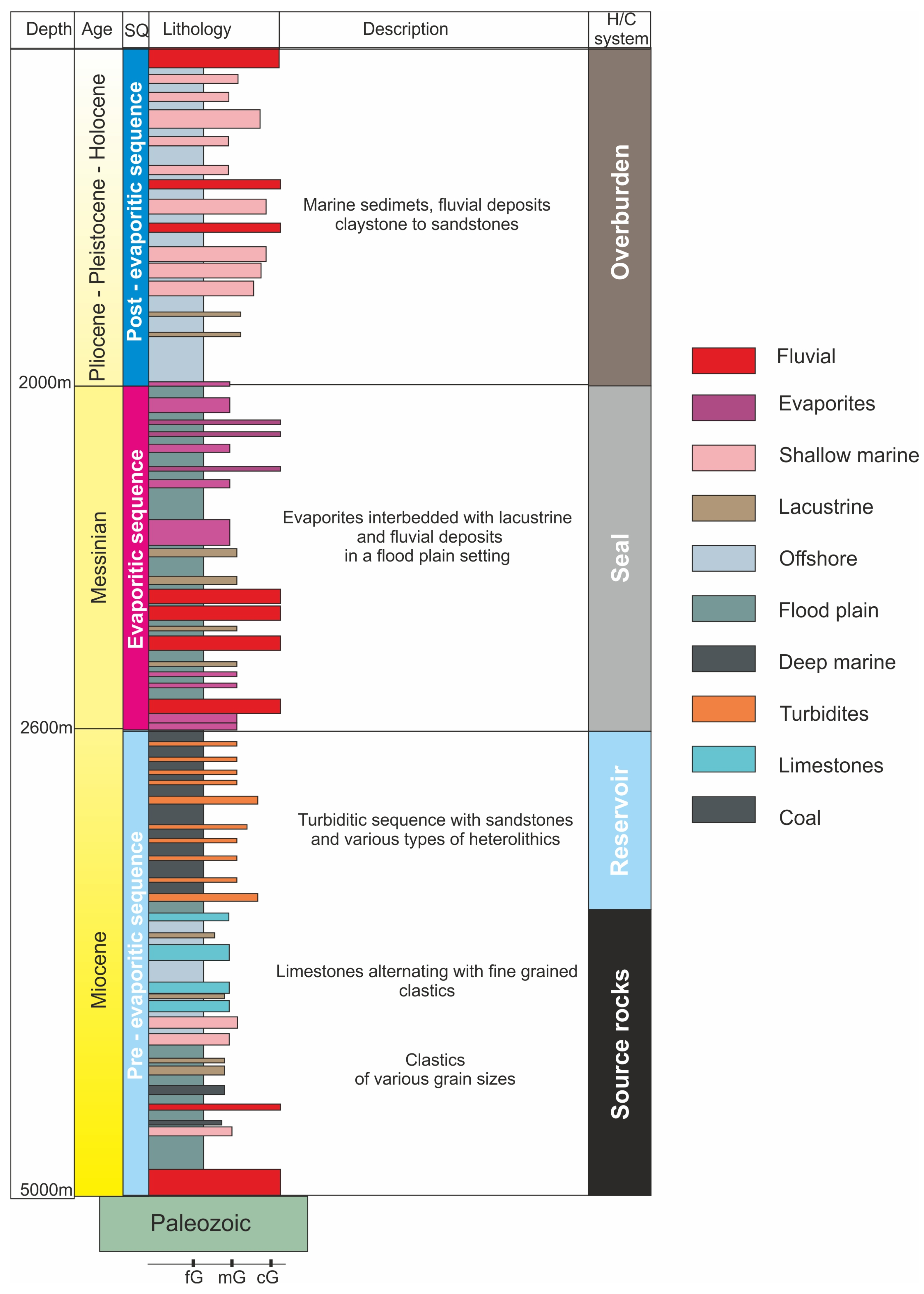
Figure 2. The stratigraphic column of the Prinos field (not in scale).
Jmse 14 00421 g002
Figure 3. The distribution of temperature (°C) with depth (m) for wells penetrating different fields: Prinos (green) and adjacent Wells (orange). The black dashed line represents the calculated geothermal gradient, while the red dashed line shows a typical geothermal gradient of 30 °C /km. The diagram illustrates the depth–temperature relationship and highlights differences in the geothermal gradient across the regions.
Jmse 14 00421 g003
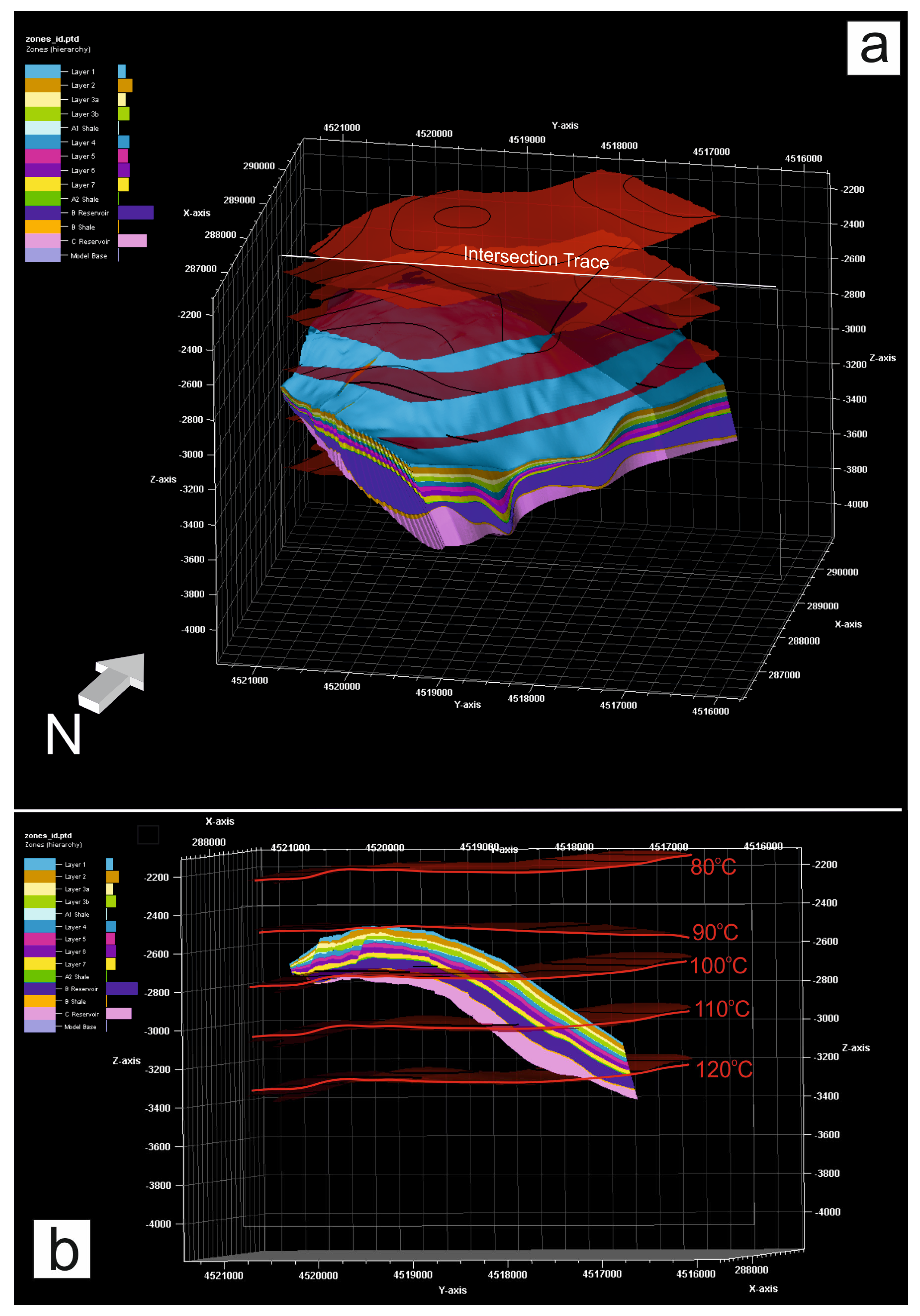
Figure 4. (a) 3D view of the Prinos static geological model showing the reservoir zones. The dark reddish surfaces represent the 80–120 °C isotherms, as calculated from corrected BHT data. The intersection trace indicates the location of the cross-section shown in panel (b). (b) Intersection plane illustrating the correlation of Prinos reservoirs and the temperature isotherms (80–120 °C). The 90 °C isotherm lies above almost the entire reservoir volume. Coordinate units are in meters.
Jmse 14 00421 g004
Figure 5. Sensitivity analysis results for (a) flow rate, (b) Heat transfer coefficient, (c) geothermal gradient. (d) production times. Temperature corresponds to wellhead.
Jmse 14 00421 g005
Figure 6. Comparison between the geothermal gradient (red line) and fluid temperature profiles across various production times. The geothermal gradient has been adjusted to equivalent bottom-hole temperature conditions.
Jmse 14 00421 g006
Figure 7. Pressure vs. depth relationship for the Prinos field, with reservoir zones distinguished by color coding. The reservoirs from the shallowest to the deepest zone are A1, A2, B, and C, respectively, as discussed in the Section 2.2. The blue and orange dashed lines represent the linear hydrostatic and lithostatic pressures, respectively.
Jmse 14 00421 g007
Figure 8. Sensitivity analysis comparison plot. Flow rate is the most critical parameter controlling wellhead temperature. The base-case scenario is indicated by the gray line with circular markers.
Jmse 14 00421 g008
Table 1. (a) Input constant parameters of Ramey calculation. (b) Input parameters for the base case scenario.
(a) Input constant parameters of Ramey calculation
Well Depth (TVD) (m)2947
Step Size (m)10
Fluid Density (kg/m3)1020
Fluid Specific Heat (J/kg*K)3700
Pipe Inner Radius (m)0.038
Bottomhole Temperature (°C)117.41
Surface Formation Temperature (°C)20
Formation Thermal Diffusivity (m2/s)1.00 × 10−6
Production Time (s)86,400
(b) Input parameters for the base case scenario.
Volumetric Flow Rates (m3/day)100
Overall heat transfer coefficient (W/m2*K)500
Geothermal Gradient (°C/m)0.035
Disclaimer/Publisher’s Note: The statements, opinions and data contained in all publications are solely those of the individual author(s) and contributor(s) and not of MDPI and/or the editor(s). MDPI and/or the editor(s) disclaim responsibility for any injury to people or property resulting from any ideas, methods, instructions or products referred to in the content.