Multi-Source Geodetic Data Fusion Using a Physically Informed Swin Transformer for High-Resolution Gravity Field Recovery: A Case Study of the South China Sea

Abstract

High-resolution marine gravity fields are critical for interpreting seafloor structure, investigating marine geodynamics, and enabling gravity-aided navigation. However, sparse shipborne observations, heterogeneous multi-source geodetic datasets, and the inability of conventional methods to handle nonlinear inversion limit accurate gravity recovery. To overcome these limitations, we propose a spectral physics-informed constraint deep-learning framework based on a multi-channel Swin Transformer to reconstruct high-resolution marine gravity anomaly fields. The model ingests multi-source geodetic inputs organized as 64 × 64 grid patches centered near each computation point and fuses them to predict the target gravity anomaly. We adopt a remove–compute–restore (RCR) strategy that isolates residual gravity signals, which improves numerical stability and accelerates training. Inputs include satellite-altimetry-derived vertical gravity gradients, vertical deflections, mean sea surface height, and topography; the model is trained on over 430,000 shipborne gravity samples from the South China Sea (0–30° N, 105–125° E). To enforce physical consistency, we embed a spectral-domain physics constraint derived from potential-field theory into the loss function; this constraint helps recover short-wavelength gravity signals. We also introduce an adaptive multi-domain multi-scale feature fusion module (AMAMFF) to improve the integration of heterogeneous inputs, and we demonstrate its benefits in experiments across complex terrain. Validation against independent shipborne gravity checkpoints yields an RMS error of 3.09 mGal, indicating a substantial performance advantage over existing deep-learning approaches and conventional gravity-field models.

1. Introduction

Gravity anomaly data are fundamental to many Earth science disciplines, including mineral exploration, tectonic structure analysis, geoid refinement, and seafloor navigation. Modern gravity measurements come from satellite altimetry, shipborne and airborne surveys, and land or marine gravimeters. Satellite altimetry yields precise sea-surface height measurements that can be inverted to produce the global marine gravity field. With accumulated multi-source altimetric datasets such as ERS-1 and Geosat, altimetry has become a primary method for constructing global gravity models [1,2,3,4]. These datasets constrain subsurface density variations and thus sharpen interpretations of structural features and resource distribution. Nevertheless, acquiring high-resolution gravity data remains technically challenging and costly.

Conventional high-resolution gravity surveys are expensive, time-consuming, and vulnerable to interference from complex topography and human activities [5,6]. For example, the marine gravimeter calibration method proposed by Pyrchla et al. [7] is complex and difficult to implement. Goodkind et al. [8,9] reported that annual maintenance for conventional gravimeters can exceed 40% of total costs. Arens et al. [10] further noted that cold-atom gravimeters still need validation to establish their feasibility for airborne use. In airborne gravity surveys, aircraft vibration, attitude changes, and atmospheric turbulence also degrade measurement accuracy [11].

Major methods for multitask gravity inversion include Cauchy-type integrals, the inverse Vening–Meinesz formula (IVM), simulated annealing, and least-squares collocation (LSC). Cauchy-type integrals convert conventional volume integrals into surface integrals for three-dimensional gravity inversion [12]. The IVM method relies on the deflections of the vertical (DOV) [13], whereas the LSC method is grounded in statistical theory and can be applied to either geoid height or DOV [14,15], while simulated annealing uses the vertical gravity gradient (VGG) [16]. Although these methods have been experimentally validated and have achieved some success, each exhibits important limitations. The Cauchy-type integral approach is highly sensitive to the accuracy of the density-contrast model and assumes horizontal homogeneity of density, permitting only vertical variations; this assumption restricts its applicability in complex geological settings. Despite its computational efficiency, applying this approach to nonlinear inversion still requires extensive iterative computation. The LSC (least-squares collocation) method requires an a priori specification of the statistical covariance function between depth and gravity anomalies and the inversion of large matrices, which creates the main computational bottleneck in practice. Simulated annealing can directly invert seafloor topography from satellite-derived vertical gravity gradient and handle strong nonlinearity, but its outcomes depend heavily on the initial depth model, which is typically constructed from shipborne data. To approach a global optimum, the algorithm needs massive iterations, imposing a heavy computational burden, and its accuracy suffers in regions with complex seafloor geology and lateral density variations due to model simplifications.

Deep learning has recently advanced rapidly in handling large-scale data and nonlinear fitting. Viswanathan et al. [17] compared traditional methods—linear regression (LM), least squares support vector machines (LSSVM), and Gaussian process regression (GPR)—and highlighted their shared limitation of weak generalization. To overcome such limits, deep learning-based joint inversion frameworks have been developed for gravity anomalies [18]. Third-generation physics-informed neural networks (PINNs) have further improved prediction stability at high altitudes [19], while physics-guided Convolutional Neural Networks (CNNs) have been proposed to model and predict seismic responses [20]. Notably, physics-informed neural networks (PINNs) have been employed to construct celestial gravity field models, thereby mitigating the convergence difficulties associated with conventional approaches [21,22]. Similarly, neural networks have been applied to high-resolution reflectivity inversion [23] and for processing irregular measurement points [24]. Zhou et al. [25] increased inversion resolution by enforcing deep weight constraints. The PTSS method strengthened boundary focusing through power–gradient constraints [26]. Finally, Fully Connected Deep Neural Networks (FC-DNNs) [27] have been applied to terrain gravity modeling, where optimizing the loss function yielded better generalization. Wu et al. [28] incorporated physical constraints into a Convolutional Networks for Biomedical Image Segmentation (U-Net) architecture to improve fitting accuracy. Niu et al. [29] refined the joint inversion objective to enable adaptive normalization of multi-source data. In the context of regional studies, a physics-constrained 3D Swin Transformer was developed to detect hot dry rock distributions in the Qinghai–Gonghe Basin [30]. Other studies have utilized multilayer perceptrons to fuse multi-source geodetic data for seafloor topography modeling in the Caribbean Sea [31]. Convolutional neural networks have also been successfully applied to merge multi-source gravity data in the Gulf of Guinea [32,33] and to recover high-precision marine gravity anomalies from satellite altimetry at the Philippine Sea–Pacific Plate boundary [34]. They also used multilayer perceptron networks to refine satellite-altimetry-derived gravity anomaly models with shipborne gravity data in the South China Sea [35]. Li et al. [36] applied convolutional neural networks to fuse multi-task satellite altimeter data in the South China Sea and thereby constructed a high-precision marine gravity field model.

In this study, we present a Swin Transformer-based method and an remove–compute–restore(RCR) technique that use the frequency-domain relationships of the gravity field as a spectral physics-informed constraint. The approach fuses positional information, terrain model from the Scripps Institution of Oceanography (SIO) (Topo 25.1), and multi-source gravity data—vertical gravity gradient, deflection of the vertical, and geoid height—to recover a gravity anomaly. First, we assemble the multi-source gravity and topographic inputs. Next, we design a Swin Transformer that accepts multi-source measurements and geographic coordinates and is trained with quality-controlled (Section 3.1) shipborne gravity observations as labels. Finally, we apply the trained Swin Transformer to generate a $1^{\prime }\times 1^{\prime }$ gravity model and assess its accuracy by comparing it with GA_MLP [35], GA_CNN [36], and other non-physics-constrained methods, as well as other gravity datasets.

The main contributions of this study are summarized as follows:

1.

We propose a physics-constrained gravity anomaly recovery framework based on multi-channel neighborhood construction and a Swin Transformer architecture, enabling effective representation learning from heterogeneous geodetic observations.

2.

A spectral physics-informed loss is introduced to explicitly enforce the frequency-domain relationship between gravity anomalies and vertical gravity gradients, improving the physical consistency of the reconstructed gravity field.

3.

An Adaptive Multi-Domain Attention Multiscale Feature Fusion (AMAMFF) module is designed to enhance cross-domain and cross-scale feature interaction within the transformer framework, effectively strengthening short-wavelength gravity signal representation and improving model robustness in regions with complex terrain.

2. Scope of Research and Data

To rigorously evaluate the performance of the proposed physics-constrained Swin Transformer, a comprehensive experimental framework is established. This section first delineates the geological and morphological characteristics of the South China Sea, justifying its selection as a complex testing ground for high-resolution gravity recovery. Subsequently, we detail the acquisition, distribution, and preprocessing protocols for the multi-source datasets—including shipborne gravity ground truth and satellite-derived potential field components—that form the data foundation for model training and validation.

2.1. Research Area

The South China Sea (SCS) lies at the junction of the Eurasian, Pacific, and Indian plates, south of the Chinese mainland and forming part of the western Pacific. As a marginal sea of the western Pacific, the SCS preserves a complex submarine topography that records the region’s formation and evolution and thus provides a natural laboratory for studying continental rifting and seafloor spreading. The gravity field of the SCS constitutes fundamental data for investigations of crustal structure and tectonic units. Accordingly, as shown in Figure 1, we define the study area as the SCS region bounded by $0^{\circ }$–${30}^{\circ }$ N and ${105}^{\circ }$–${125}^{\circ }$ E, and we employ multi-source gravity and bathymetric datasets to reconstruct the regional gravity field. To mitigate edge effects, the computation automatically extends the domain by $1^{\circ }$ outward. The seabed morphology displays pronounced zonation: shallow continental shelves occur in the north, west, and south and extend seaward to continental slopes that host plateaus, seamounts, canyons, troughs, and trenches. The eastern island arc is relatively narrow and lies adjacent to trenches and troughs, while the central sector consists of deep-water basins with broad, plain-like floors that are sporadically punctuated by isolated seamounts. These varied features make the region a rigorous testbed for validating deep-learning approaches to gravity recovery.

2.2. Using the Dataset

A robust deep learning model relies on high-quality, multi-source geophysical inputs. This section categorizes the datasets employed in this study into two primary groups: shipborne gravity measurements, which serve as the ground truth labels for training and validation, and satellite-derived potential field components (e.g., vertical gravity gradient, geoid height), which act as the model’s feature inputs. The acquisition sources, resolution, and specific preprocessing protocols for each dataset are detailed below to ensure data reliability and methodological transparency.

2.2.1. Shipborne Gravity Data

Shipborne gravity measurements provided the primary training data for this study. We obtained these observations from the U.S. National Centers for Environmental Information. The training dataset consisted mainly of longitude, latitude, and free-air gravity anomaly values. We selected 21 shipborne gravity survey lines spanning multiple campaigns. Data from 1980 to 1985 were acquired by the Institute of Physics of the Earth (IFZ), Russian Academy of Sciences (AN); Lamont-Doherty Geological Observatory (USA); Bundesanstalt für Geowissenschaften und Rohstoffe (Germany); and Institut Français de Recherche pour l’Exploitation de la Mer (IFREMER, France). Data from 1986 to 1990 were collected by the Japan National Institute of Polar Research (Japan); Bundesanstalt für Geowissenschaften und Rohstoffe (Germany); and the University of Hawaii, SOEST, and Princeton University (USA). Data from 1991 to 1995 were obtained by the University of Hawaii, SOEST; Princeton University; and Lamont-Doherty Earth Observatory (USA). After quality control (Section 3.1), the integrated dataset comprised 432,855 observations (Figure 2a). For model development, we randomly sampled 80% of the computation points by survey-line ID to form the training set (Figure 2b). We held out 20% as a validation set for iterative model optimization. The remaining data (Figure 2b) were reserved as an independent test set and were completely excluded from training.

2.2.2. Reference Gravity Model and Terrain Model

The Earth Gravitational Model 2008 (EGM2008) is used here as the reference gravity model; specifically, the version expanded to degree and order 2190 is adopted [14,37,38]. Using the remove–restore technique (RCR), we separate the gravity field into long-wavelength and short-wavelength residual components [39]. The RCR procedure is applied to four types of input data: vertical gravity gradient, deflection of the vertical (meridional component and prime vertical component), geoid height, and shipborne gravity anomalies. This generates the corresponding residual fields used for model training.

Figure 3 presents the geoid height model, a global 1-arcminute dataset of geoid undulations that quantifies the vertical offset of the geoid relative to a reference ellipsoid (i.e., geoid height anomalies). Jointly released by the U.S. National Geospatial-Intelligence Agency and the U.S. National Oceanic and Atmospheric Administration, the model was constructed from satellite gravity measurements, airborne gravity surveys, satellite radar altimetry, and terrestrial gravity observations. The Global Topography and Geophysical Fields (GTGF) series comprises 1-arcminute global datasets produced by the Scripps Institution of Oceanography. These datasets cover terrestrial topography and ocean bathymetry, free-air gravity anomalies, vertical gravity gradients, and the east–west and north–south components of vertical deflection. The GTGF series is derived from multiple observation types, including multibeam and single-beam shipborne soundings, multi-mission satellite radar altimetry (e.g., CryoSat-2, AltiKa, Sentinel-3), airborne gravity surveys, and publicly available GEBCO grids, and it was generated using waveform retracking, downward continuation filtering, and depth-dependent spatial filtering.

3. Method

This chapter presents the methodological framework for high-resolution marine gravity recovery. We first describe the data preprocessing pipeline, including quality control of shipborne observations and the remove–compute–restore (RCR) procedure used to isolate short-wavelength residual signals. We then introduce the Swin Transformer backbone enhanced with the Adaptive Multi-Domain Attention Multiscale Feature Fusion (AMAMFF) module. Finally, we define a spectral Laplacian consistency loss as a physics-guided regularization term and evaluate its effect through ablation and comparative experiments.

3.1. Data Preprocessing

This study used shipborne gravity measurements collected since 1980 and addressed residual systematic biases among survey tracks. Although the raw data had already received Eötvös and instrument-drift corrections, systematic errors persist across cruises because observation units, instrument models, and operational platforms differ [40]. To improve data quality, we used the EGM2008 gravity field model as a prior constraint for quality control; both datasets reference the WGS84 ellipsoid. First, records with free-air gravity anomaly values equal to 0 or NaN were removed, eliminating approximately 34.67% of the original observations. We then computed residuals between the EGM2008 model anomalies and the measured data and evaluated their mean and standard deviation (STD). Observations with residuals exceeding three times the standard deviation were treated as outliers and removed. When the residual mean deviated significantly from zero, we interpreted this as evidence of systematic bias and applied cruise-specific mean corrections. Some historical surveys in the study area showed larger systematic biases, likely due to early acquisition dates and lower measurement precision; for example, cruise V3613 had an outlier removal rate of 12.78%, and SO23 had 9.79%. Initially, 678,677 shipborne gravity records were collected for the region; after quality control, 432,855 valid points remained, corresponding to an overall outlier removal rate of 2.49%. These filtered data will be used for subsequent model training and prediction. SSE denotes the residuals data.

Furthermore, according to RCR theory, the gravitational field can be decomposed into a long-wavelength fundamental field and a short-wavelength residual field, as shown below:

$$\Delta \mathrm{g}(x,y)=\Delta {\mathrm{g}}_{\mathrm{res}}(x,y)+\Delta {\mathrm{g}}_{\mathrm{EGM}2008}(x,y)$$

(1)

In the equation, $\Delta {\mathrm{g}}_{\mathrm{res}}(x,y)$ denotes the short-wavelength residual gravity field and $\Delta {\mathrm{g}}_{\mathrm{EGM}2008}(x,y)$ represents the long-wavelength reference gravity obtained from the EGM2008 model. In the Swin Transformer approach, the short-wavelength component of shipborne gravity measured at training stations serves as an input feature. Before training, the EGM2008 gravity anomaly at each station is subtracted from the shipborne measurement to yield the residual gravity anomaly.

3.2. Swin Transformer Model for Gravity Recovery

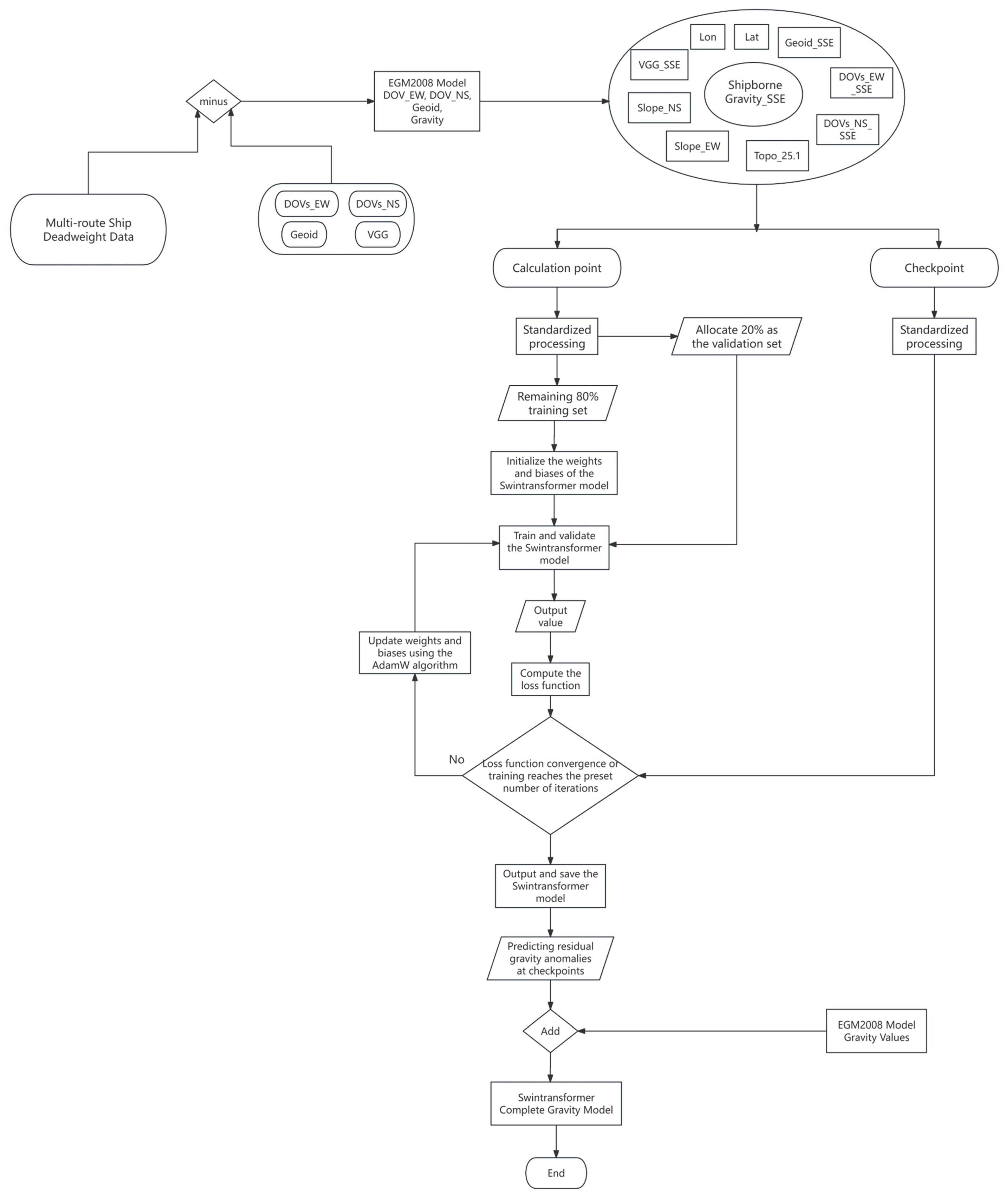
We present a physics-guided deep-learning framework for gravity-field recovery, built on a Swin Transformer backbone and an Adaptive Multi-domain Attention Multiscale Feature Fusion (AMAMFF) module. The AMAMFF module uses a symmetric U-shaped decoder to preserve high-frequency details and combines channel attention, self-attention, spatial attention, and frequency-domain attention for dynamic fusion of multi-source geodetic inputs. To introduce physical guidance, we add a spectral Laplacian residual term to the training objective, where spectral derivatives are used to compute Laplacian consistency penalties. The final hybrid loss jointly optimizes data fidelity and physics-guided regularization for high-resolution gravity anomaly reconstruction.

3.2.1. Adaptive Multi-Domain Attention Multiscale Feature Fusion Module

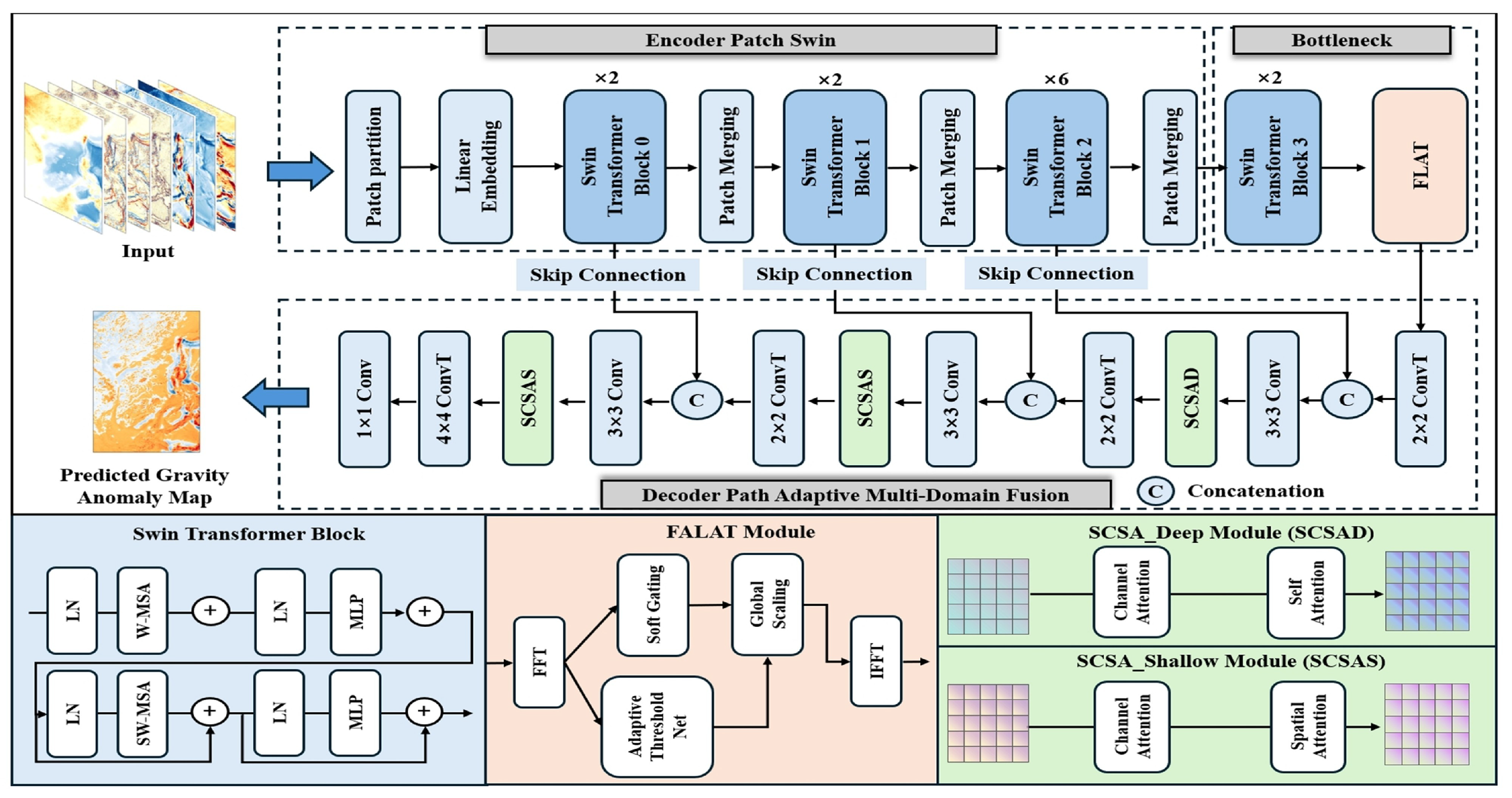
We refer to the Adaptive Multi-domain Attention Multi-scale Feature Fusion module as AMAMFF. To mitigate the loss of high-frequency spatial details caused by the downsampling operations in the Swin Transformer backbone, we design a symmetric U-Net Multi-Scale Feature Fusion Module, as illustrated in Figure 4.

This decoder structure adopts a U-Net-like architecture to bridge the gap between the deep semantic representations extracted by the encoder and the shallow geometric details required for high-resolution gravity field reconstruction.

The Channel Attention mechanism serves a critical role in handling the potential multicollinearity among multi-source inputs (e.g., VGG, DOV, and Geoid). In traditional inversion methods like Least Squares Collocation (LSC), highly correlated inputs can lead to ill-conditioned covariance matrices and unstable solutions. However, our deep learning framework addresses this through Adaptive Feature Recalibration. The Channel Attention module acts as an “Adaptive Soft Selector”. It learns a weight vector $\mathbf{w}\in {[0,1]}^C$ through the global average pooling and fully connected layers (Equation (6)). This allows the network to dynamically suppress redundant information and amplify informative features based on the local context. For instance, in regions with sharp topographic changes, the network can assign higher weights to the VGG channel (which is sensitive to high-frequency edges) while downweighting the smoother Geoid channel, and vice versa. This mechanism effectively converts the challenge of multicollinearity into an advantage of multi-view feature fusion.

The Swin Transformer backbone generates hierarchical feature maps $\{F_0,F_1,F_2,F_3\}$ at four distinct stages. These features possess decreasing resolutions (ranging from ${\displaystyle \frac{1}{4}}$ to ${\displaystyle \frac{1}{16}}$ of the input size) and increasing channel dimensions ($C,2C,4C,8C$). To facilitate efficient fusion, we first utilize $1\times 1$ convolutional layers to project features from all stages into a unified hidden dimension $D_h$ (set to 64 in our experiments), ensuring channel alignment:

$${\widehat{\mathbf{F}}}_i={\mathrm{Conv}}_{1\times 1}\left({\mathbf{F}}_i\right),i\in \{0,1,2,3\}$$

(2)

where ${\widehat{\mathbf{F}}}_i$ denotes the projected standardized feature map at stage i. The decoding process follows a bottom-up restoration pathway. As shown in Figure 5, the reconstruction starts from the deepest bottleneck feature ${\widehat{\mathbf{F}}}_3$. For each subsequent stage i, the decoder feature ${\mathbf{D}}_i$ is generated by fusing the upsampled feature from the deeper layer (${\mathbf{D}}_{i+1}$) with the corresponding encoder feature (${\widehat{\mathbf{F}}}_i$) via lateral skip connections.

Before upsampling, the Stage 2 bottleneck feature F₃ is first refined by a frequency-domain attention module. This module adaptively amplifies high-frequency components associated with gravity anomalies while suppressing noise. The procedure is as follows:

First, the features are transformed into the frequency domain using the Fast Fourier Transform (FFT):

$$X(u,v)=\mathcal{F}\left\{{\widehat{F}}_3\right\}$$

(3)

Second, a lightweight adaptive-threshold network is employed to learn frequency-domain masks, enabling the soft gating and global scaling of distinct frequency components:

$$X^{\prime }(u,v)=X(u,v)\odot \sigma \left(W_f·\left|X(u,v)\right|+b_f\right)$$

(4)

Finally, the optimized features are restored to the spatial domain via the inverse Fourier transform (IFFT):

$${\widehat{F}}_3^{\mathrm{enhanced}}={\mathcal{F}}^{-1}\left\{X^{\prime }\right\}$$

(5)

Here, $\mathcal{F}$ and ${\mathcal{F}}^{-1}$ denote the two-dimensional Fourier transform and its inverse, respectively, $W_f$ and $b_f$ are learnable parameters, and ⊙ denotes element-wise multiplication. The enhanced feature ${\widehat{F}}_3^{\mathrm{enhanced}}$ serves as the decoder’s initial input and is denoted as $D_3$.

Attention modules: Prior to describing Feature Integration, we first define the three attention mechanisms employed.

(1)

Channel Attention

Employing a squeeze-and-excitation architecture, spatial information is first compressed via global average pooling. Subsequently, two fully connected layers combined with a Sigmoid function generate the channel weight vector:

$$z=\mathrm{GAP}\left(x\right),s=\sigma \left(W_2·\mathrm{ReLU}\left(W_{1}z\right)\right)$$

(6)

where x denotes the input feature, GAP denotes global average pooling, $W_1$ and $W_2$ are learnable weights, and $\sigma$ is the Sigmoid function. The weighted feature is

$$A_{\mathrm{channel}}\left(x\right)=s\odot x$$

(7)

(2)

Self-Attention

This introduces a lightweight global context modeling module that aggregates long-range dependencies through a query–key–value mechanism:

$$Q=x{W}_Q,K=x{W}_K,V=x{W}_V$$

(8)

$$A_{\mathrm{self}}=\mathrm{Softmax}\left({\displaystyle \frac{Q{K}^{\mathrm{T}}}{\sqrt{d_K}}}\right)V$$

(9)

where $W_Q$, $W_K$, and $W_V$ are the projection weight matrices, and $d_K$ denotes the dimensionality of the keys.

(3)

Spatial Attention

This generates spatial weight maps through convolutional layers to highlight important regions:

$$M_s=\sigma \left({\mathrm{Conv}}_{7\times 7}\left(\left[x_c^{\mathrm{avg}},x_c^{\max }\right]\right)\right)$$

(10)

where $x_c^{\mathrm{avg}}$ and $x_c^{\max }$ denote the results of average and max pooling along the channel dimension, respectively. The weighted output is

$$A_{\mathrm{spatial}}=M_s\odot x$$

(11)

Specifically, the fusion operation consists of three steps:

1.

Upsampling: The deeper feature map is upscaled by a factor of 2 using a transposed convolution layer (ConvTranspose2d).

2.

Concatenation: The upsampled feature is concatenated with the skip-connected encoder feature ${\widehat{\mathrm{F}}}_i$ along the channel dimension.

3.

Feature Integration: The concatenated tensor is processed by a fusion block consisting of a $3\times 3$ convolution, Batch Normalization (BN), and a GELU activation function to smooth aliasing effects and integrate contextual information.

Mathematically, this recursive fusion is defined as

$${\mathrm{D}}_i={\mathcal{B}}_{\mathrm{fus}}^{\mathrm{attn}}\left(\mathrm{Concat}\left[{\widehat{\mathrm{F}}}_i,\mathrm{ConvTranspose}\left({\mathrm{D}}_{i+1}\right)\right]\right),i\in \{2,1,0\}$$

(12)

where ${\mathcal{B}}_{\mathrm{fus}}^{\mathrm{attn}}$ represents the fusion block

$${\mathcal{B}}_{\mathrm{fus}}^{\mathrm{attn}}\left(x\right)=\mathrm{GELU}\left(\mathrm{BN}\left({\mathrm{Conv}}_{3\times 3}\left({\mathrm{F}}_i^{\mathrm{out}}\right)\right)\right)$$

(13)

where ${\mathrm{F}}_i^{\mathrm{out}}$ is defined by the following conditional expression:

$$F_i^{\mathrm{out}}=\left\{\begin{array}{cc}{\mathcal{A}}_{\mathrm{self}}\left({\mathcal{A}}_{\mathrm{channel}}\left(x\right)\right),\hfill & i=2\hfill \\ {\mathcal{A}}_{\mathrm{spatial}}\left({\mathcal{A}}_{\mathrm{channel}}\left(x\right)\right),\hfill & i=1,0\hfill \end{array}\right.$$

(14)

After iterative fusion, the final decoder feature map ${\mathbf{D}}_0$ reaches a resolution of $16\times 16$. To generate the final output, we apply a final $4\times 4$ transposed convolution to upsample the feature map to the original input resolution ($64\times 64$). A linear regression head (implemented as a $1\times 1$ convolution) is then applied to map the high-dimensional features to the single-channel predicted gravity anomaly map $\widehat{\mathbf{G}}$:

$$\widehat{\mathbf{G}}={\mathrm{Conv}}_{1\times 1}\left({\mathrm{ConvTranspose}}_{4\times 4}\left({\mathbf{D}}_0\right)\right)$$

(15)

Table 1. Model Configuration Table.

Module	Parameter	Value
Input	Input Resolution	$64\times 64$
	Input Channels	9
	Patch Size (Raw)	$4\times 4$ (grid points)
Encoder	Backbone Type	Swin Transformer (Custom Tiny)
	Patch Size (Embed)	2
	Window Size	4
	Embed Dimension (C)	96
	Stage Depths	$(2,2,6,2)$
	MLP Ratio	4
	QKV Bias	TRUE
	Structure	Symmetric U-Net with Skip Connections
Decoder	Fusion Stages	0, 1, 2, 3
	Hidden Dimension	64
	Multiscale Fusion	TRUE
	Channel Attention	8
	Spatial Attention	True
	Self Attention	8
	FALAT	True
Physics	Physics Loss Weight ($\lambda$)	$0.1$
	Grid Distance	$0.25$ (km/unit approx)
Training	Optimizer	AdamW
	Learning Rate	$1\times {10}^{-4}$ (0.0001)
	Batch Size	12
	Max Epochs	80
	Early Stop Patience	10 epochs
	Spatial Split Bin	$1^{\circ }\times 1^{\circ }$ ($1/60$ degree)

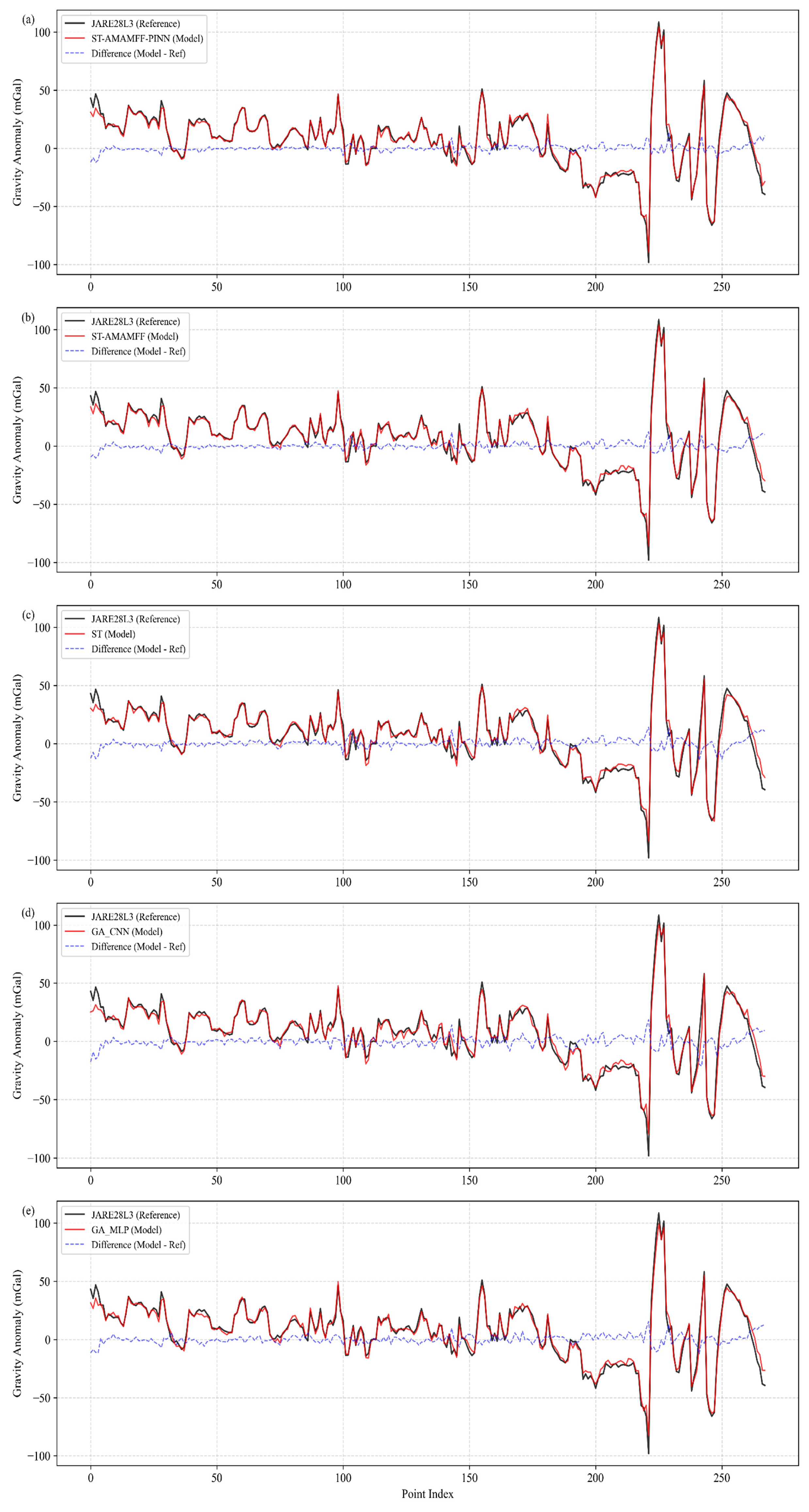
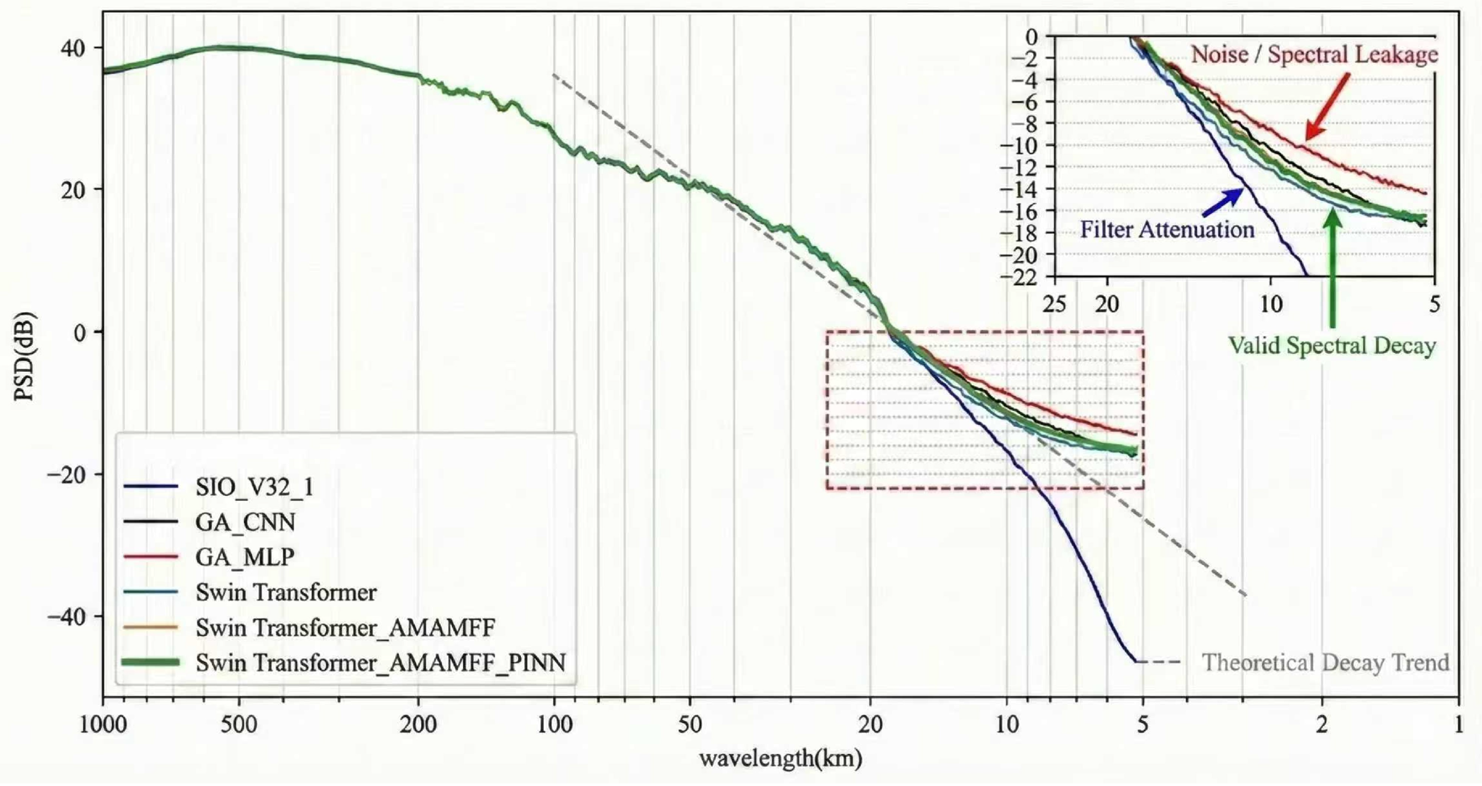
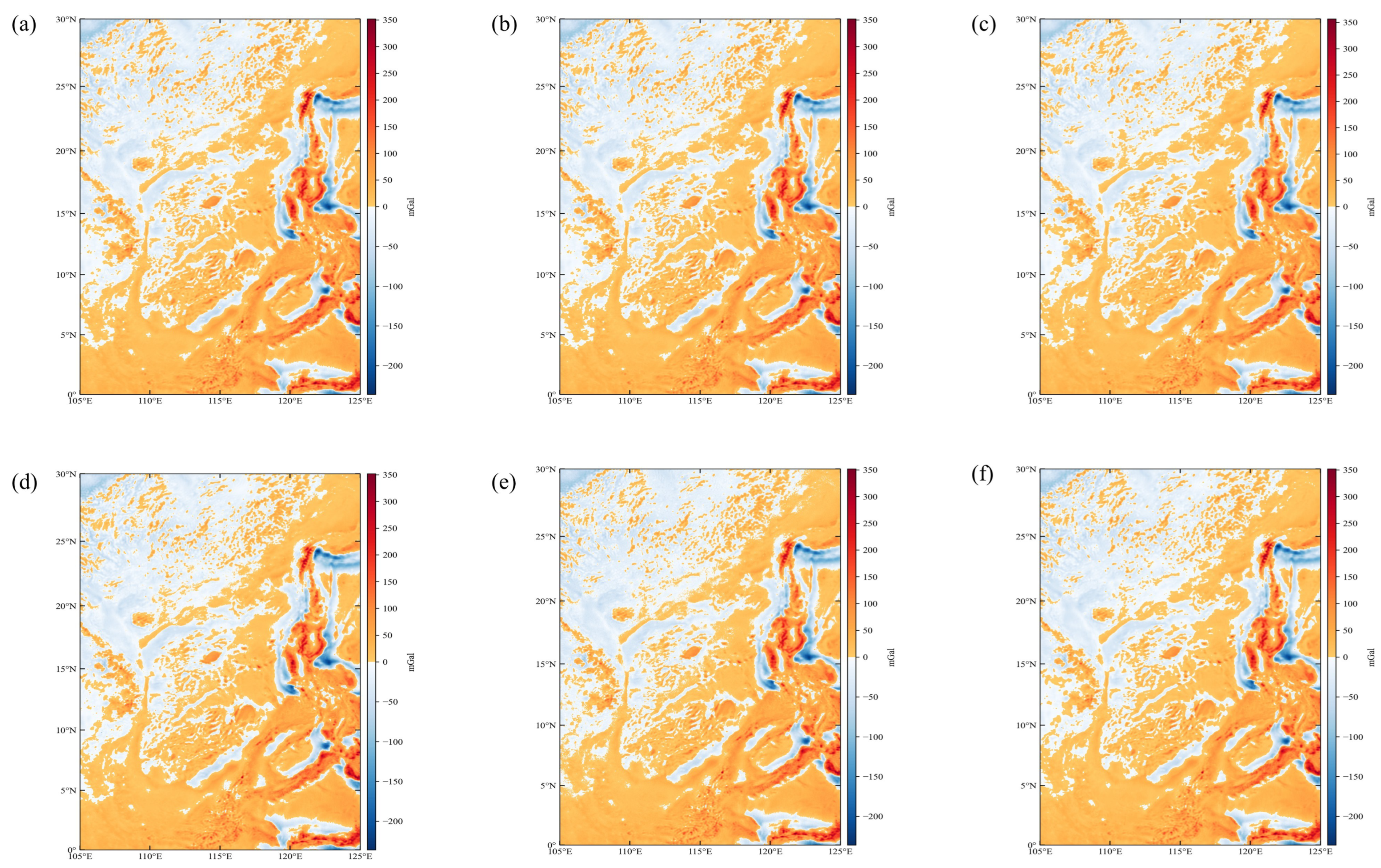
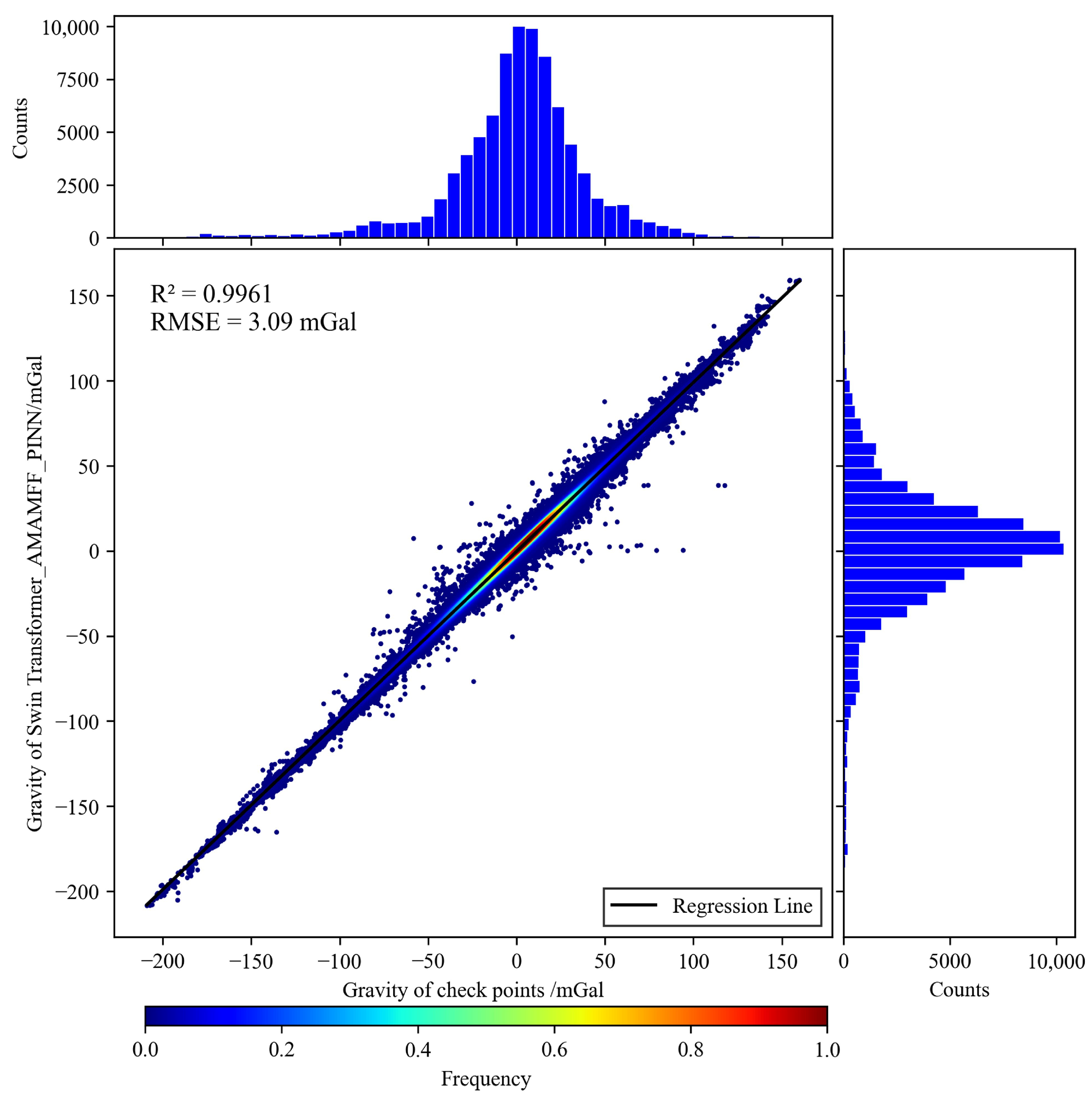
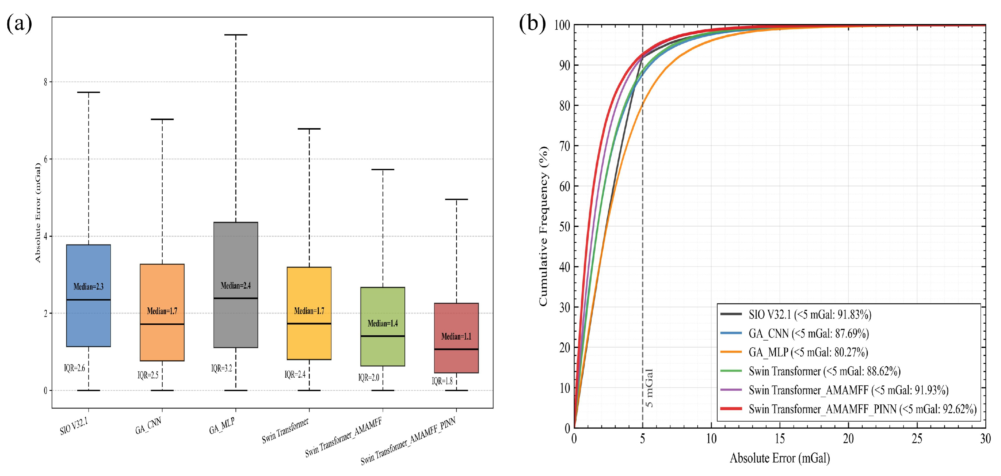
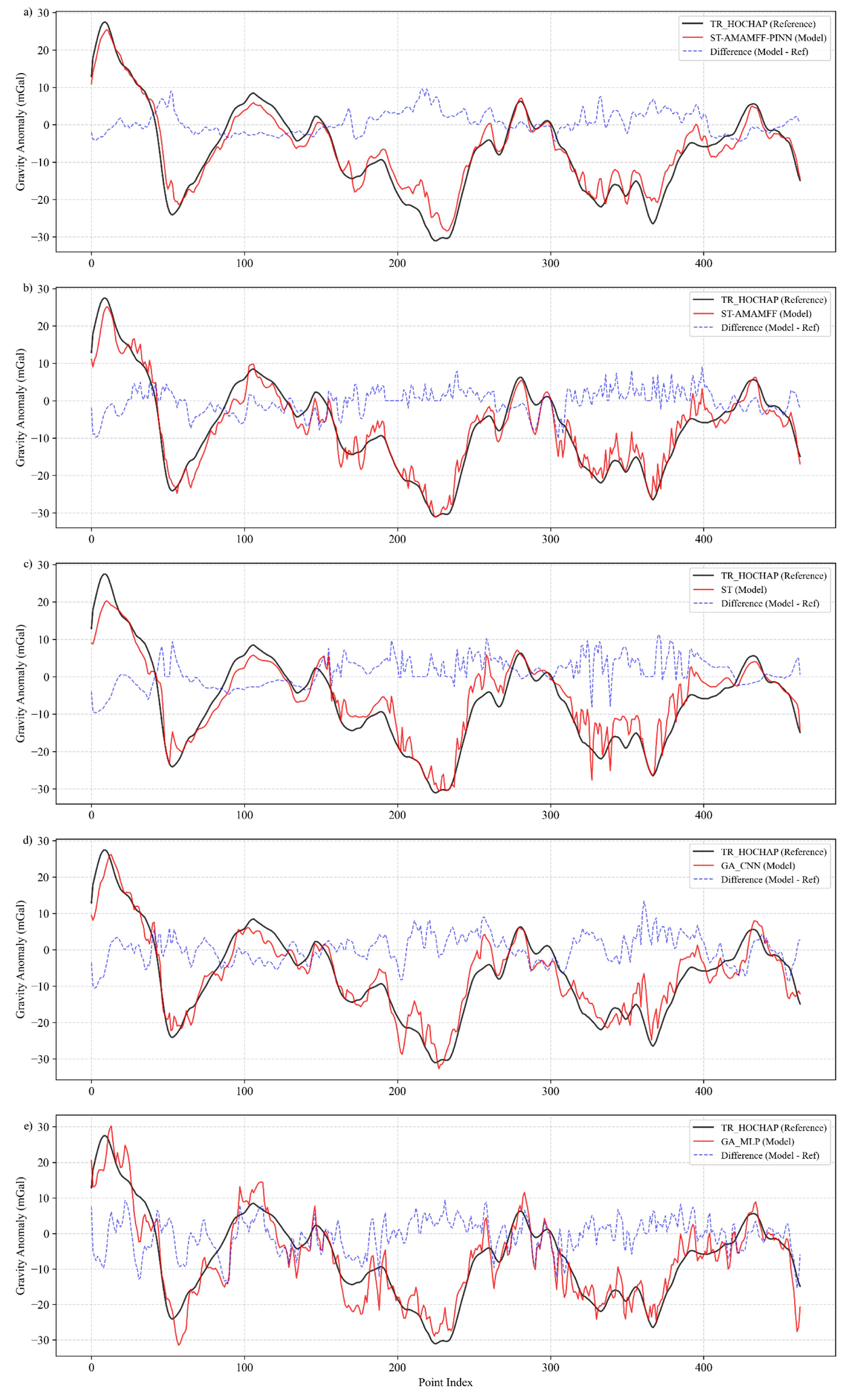
shows that the multi-domain attention modules in AMAMFF are not stacked merely to deepen the network but are tailored to the specific characteristics of gravity anomaly data. Channel attention reweights heterogeneous geophysical inputs, while spatial attention highlights local gravity features and self-attention captures long-range structural correlations. Frequency-domain attention suppresses nonphysical high-frequency noise by exploiting the spectral properties of the potential field. Applied sequentially, these modules progressively refine features rather than redundantly amplifying them, a distinction that appears in the comparative performance of the ST, ST-AMAMFF, and ST-AMAMFF-PINN models.

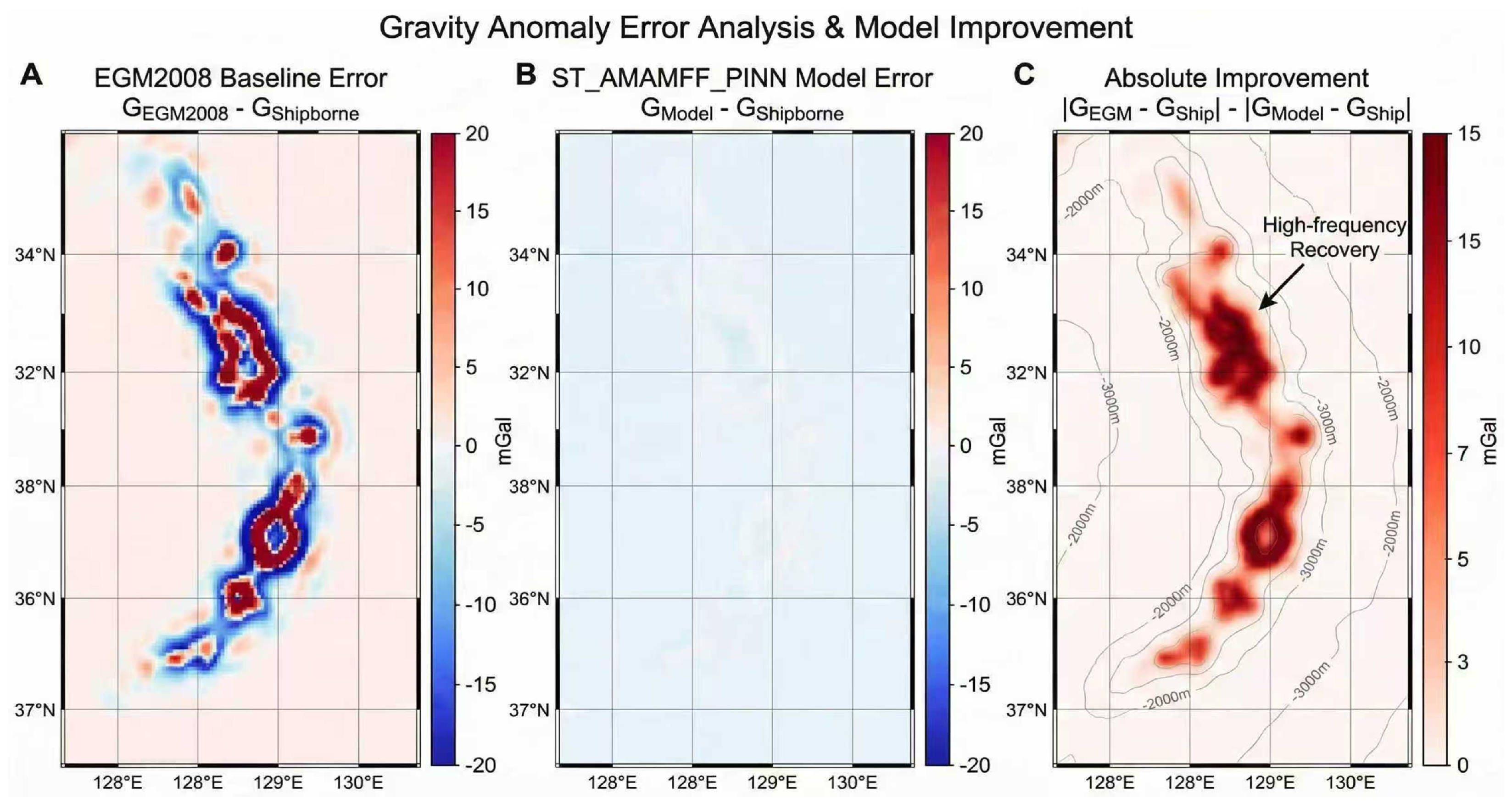
By leveraging this multi-scale fusion strategy, the network effectively recovers the fine-grained gravity signals associated with topographic variations while maintaining the global trends captured by the deep transformer layers.

3.2.2. Improvements to the Loss Function

To combine shipborne gravity measurements with prior geophysical knowledge, this study develops a hybrid loss function that integrates data-driven and physics-based constraints. The loss comprises a data term ${\mathcal{L}}_{\mathrm{MSE}}$ and a physics term ${\mathcal{L}}_{\mathrm{physics}}$, and its overall form is given by the following equation:

$${\mathcal{L}}_{\mathrm{total}}={\mathcal{L}}_{\mathrm{MSE}}+\lambda {\mathcal{L}}_{\mathrm{physics}}$$

(16)

Among these, $\lambda$ is the hyperparameter that balances the two components. The data items use mean square error (MSE) to measure the discrepancy between predicted values and true values obtained from ship surveys:

$${\mathcal{L}}_{\mathrm{MSE}}={\displaystyle \frac{1}{N}}\sum _{k=1}^N{∥{\mathbf{P}}_i(c,c)-{\mathbf{T}}_i∥}^2$$

(17)

where ${\mathbf{P}}_i$ represents the predicted residual map for the i-th sample, $c=\lfloor {\displaystyle \frac{n}{2}}\rfloor$ denotes the center pixel index, and ${\mathbf{T}}_i$ indicates the ground truth residual from the shipborne measurement. The physics term incorporates the frequency-domain relationship of the gravitational field as a physical constraint. Based on phase field theory [41,42], this ensures that the predicted results comply with physical laws. The residual map ${\mathbf{P}}_i(c,c)\in {\mathbb{R}}^{N\times N}$ of the predicted gravity anomaly is converted to the frequency domain:

$$G(u,v)=\mathcal{F}\left\{{\mathbf{P}}_i(c,c)\right\}$$

(18)

where $(u,v)$ represents the frequency domain coordinate and $\mathcal{F}$ denotes the two-dimensional Fourier transform. The vertical second derivative of gravity anomaly $\Delta g$ can be approximated in the frequency domain as [39,41]

$$V_{zz}(u,v)=2\pi \sqrt{u^2+v^2}·\Delta g(u,v)$$

(19)

Therefore, the vertical gradient calculated from the predicted gravity anomaly is

$$V_{zz}(u,v)=2\pi \sqrt{u^2+v^2}·G(u,v)$$

(20)

The predicted vertical gradient in the spatial domain is obtained through the inverse Fourier transform:

$$V_{zz}^{\mathrm{pred}}={\mathcal{F}}^{-1}\left\{V_{zz}(u,v)\right\}$$

(21)

where ${\mathcal{F}}^{-1}$ denotes the inverse Fourier transform. Compare $V_{zz}^{\mathrm{pred}}$ with $V_{zz}^{\mathrm{obs}}$ in the input channel:

$${\mathcal{L}}_{\mathrm{physics}}={\displaystyle \frac{1}{N\times N}}\sum _{i=1}^N\sum _{j=1}^N{∥V_{zz}^{\mathrm{pred}}(i,j)-V_{zz}^{\mathrm{obs}}(i,j)∥}^2$$

(22)

where $(i,j)$ represents the coordinate position in the spatial domain.

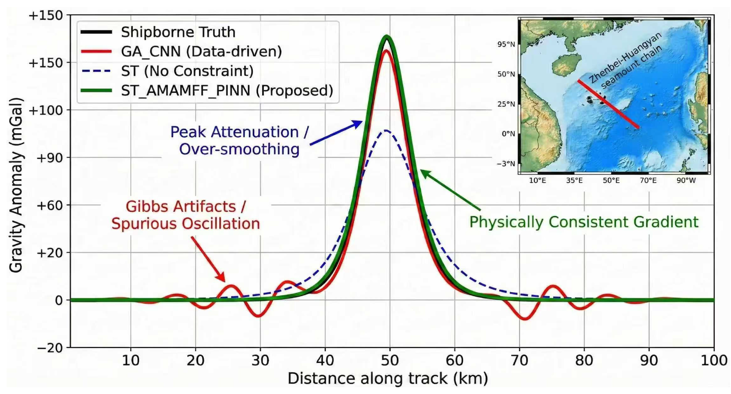
Where ${\mathcal{L}}_{\mathrm{data}}$ (Equation (17) in original text) ensures data fidelity at shipborne observation points, while ${\mathcal{L}}_{\mathrm{physics}}$ constrains the solution space to the set of valid harmonic functions. By minimizing Equation (16), the network is prevented from generating non-physical high-frequency artifacts that violate Laplace’s equation.

Sensitivity Analysis of the Physics-Guided Regularization Weight ($\lambda$)

The hyperparameter $\lambda$ in Equation (16) balances data fidelity (${\mathcal{L}}_{\mathrm{data}}$) and physical consistency (${\mathcal{L}}_{\mathrm{physics}}$). We conducted a sensitivity analysis by varying $\lambda$ from 0.01 to 1.0.

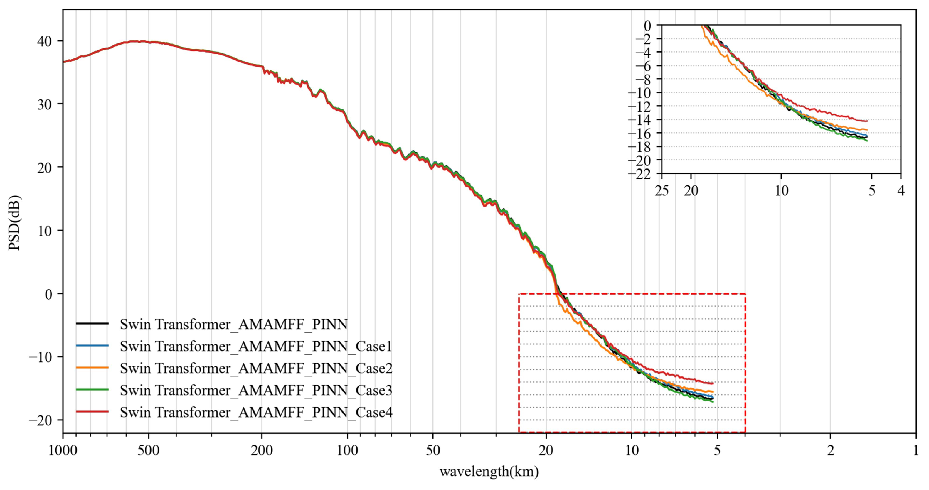
Small $\lambda$ (<0.05): The model converges faster to the data but exhibits high-frequency noise in the derivatives, indicating insufficient physical regularization.

Large $\lambda$ (>0.5): The total loss is dominated by the gradient constraint, leading to “over-smoothing”, where sharp peak signals (e.g., seamounts) are attenuated.

Optimal $\lambda$ ($0.1$): Empirical results show that $\lambda =0.1$ provides the best trade-off, minimizing RMSE while maintaining sharp, physically consistent gradients.

3.2.3. Complete Model Architecture

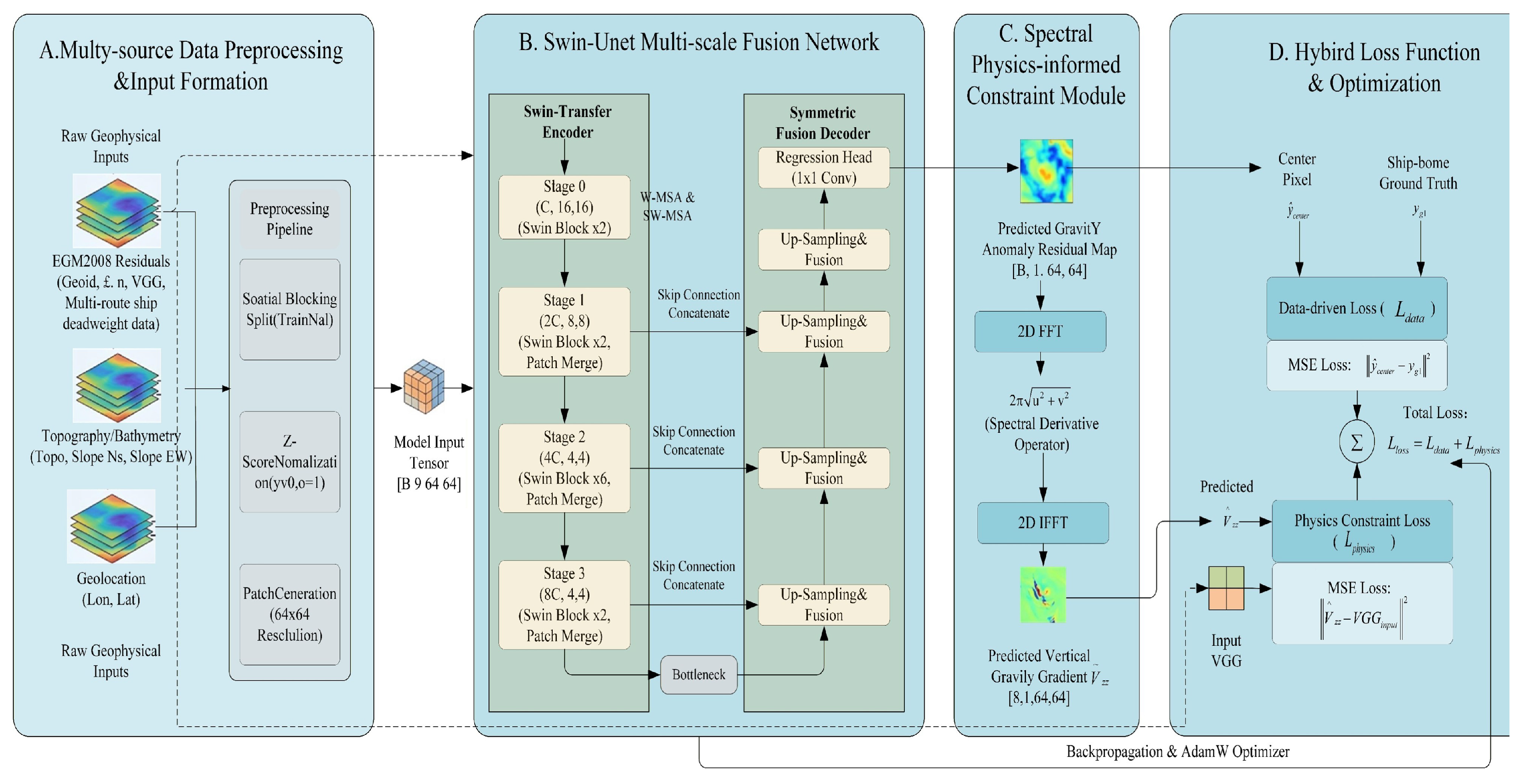
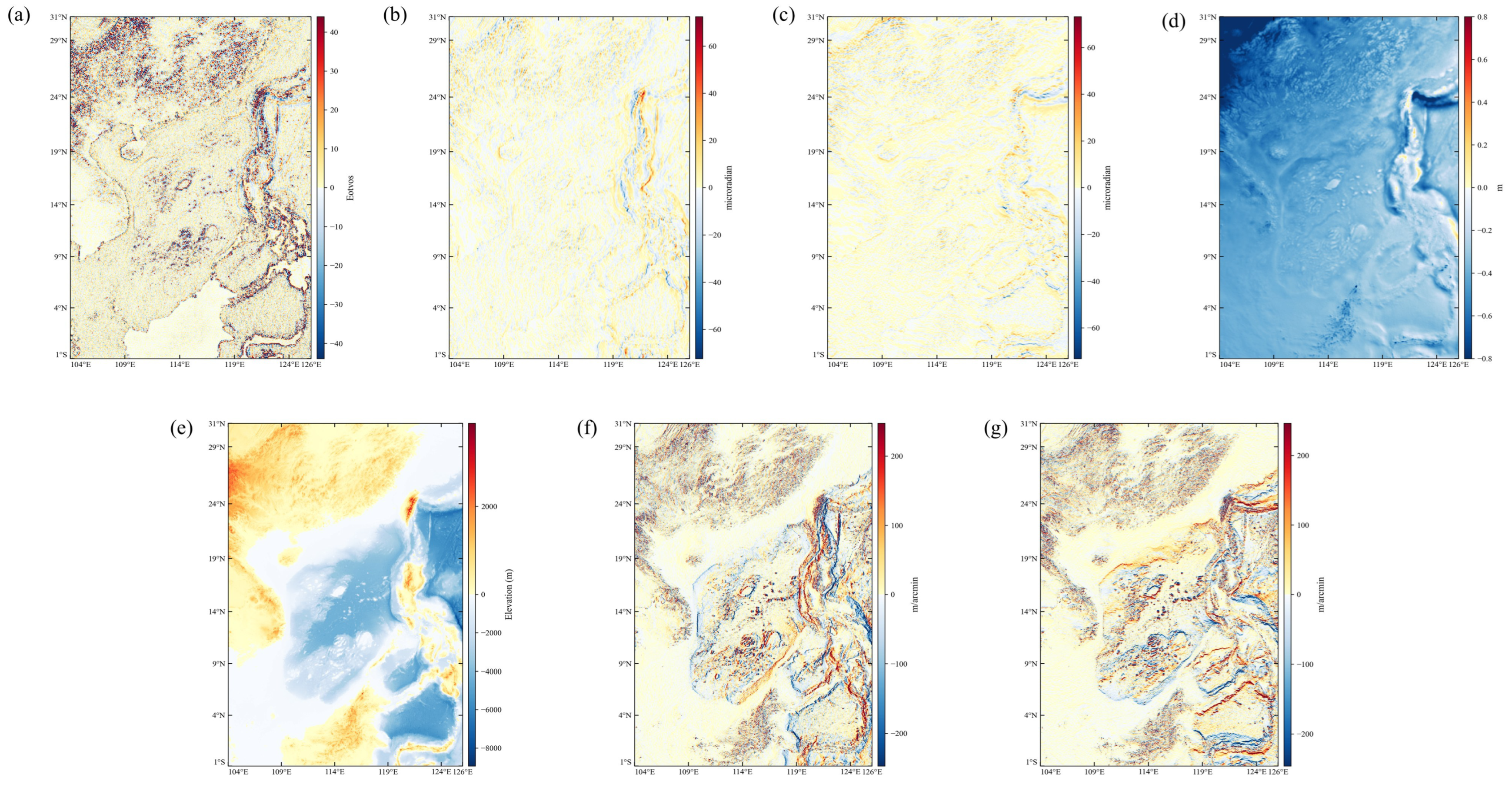
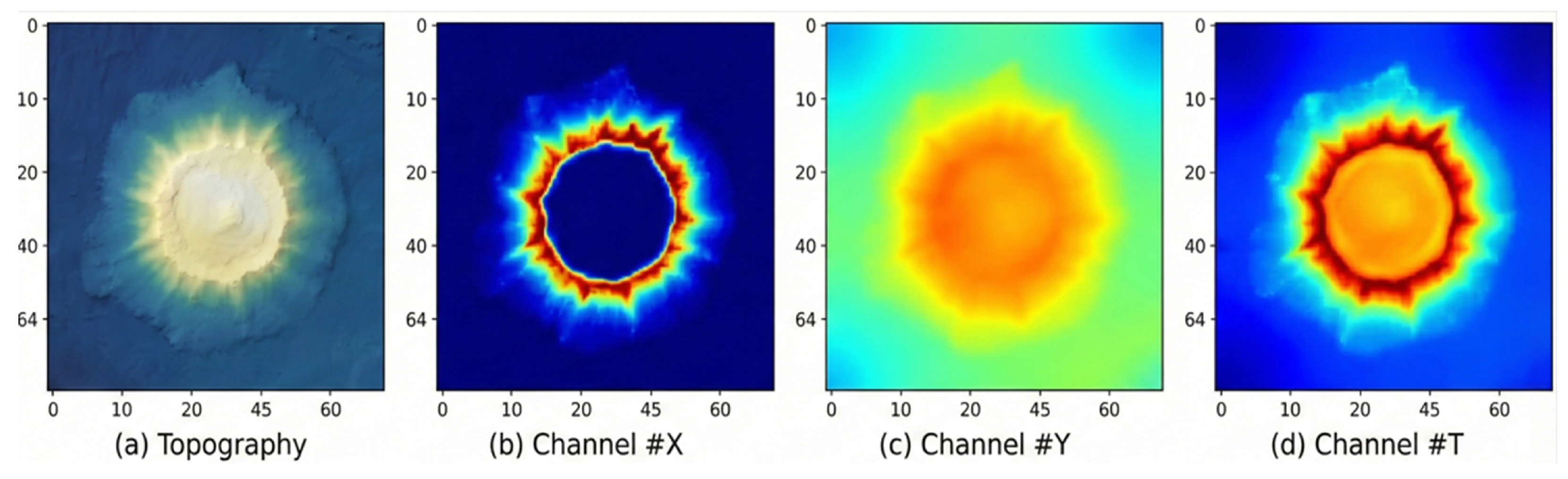
The proposed framework is a physics-constrained deep learning architecture for reconstructing gravity anomalies and comprises four stages (Figure 5). The first stage prepares multisource inputs and constructs the network input to reduce data heterogeneity through the fusion of diverse geophysical measurements. The DataEngine assembles nine channels: residuals of multisource geodetic data (geoid height, vertical gravity gradient, and deflection of the vertical), topography, seafloor topographic slope, and explicit geographic coordinates. Residuals from multi-route shipborne gravity surveys are used as training labels. To make these data suitable for deep learning, the spatial domain is partitioned into blocks for training–test separation, and each channel is standardized by Z-score normalization. Finally, input subgraph blocks are generated and upsampled when required to preserve local spatial context.

The framework centers on a Swin-UNet multi-scale fusion network augmented with an adaptive multi-domain attention mechanism (Swin-UNet with Adaptive Multi-Domain Attention for Multi-scale Fusion). The encoder employs a Swin Transformer backbone (Stage 0 to Stage 3) to extract multi-scale semantic features. It uses multi-head self-attention in windowed and shifted-window configurations and progressively reduces spatial resolution through patch-merging layers. We term the module the adaptive multi-domain attention fusion decoder. Using transposed-convolution upsampling and skip connections, it fuses deep semantic features with shallow terrain texture features across multiple scales to restore spatial detail. The module implements a hierarchical attention strategy. At the bottleneck, frequency-domain attention performs global frequency enhancement of features. During subsequent upsampling and fusion, attention combinations are applied adaptively by feature hierarchy: in the deep fusion stage (${\mathrm{stage}}_2$), channel attention followed by self-attention is applied sequentially to strengthen global context modeling, while in the shallow fusion stages (${\mathrm{stages}}_1$ and ${\mathrm{stages}}_0$), channel attention followed by spatial attention is applied sequentially to enhance local detail reconstruction. This hierarchical, adaptive attention mechanism improves the network’s ability to capture both local details and global dependencies in gravity field signals. A final regression head projects the fused features onto the residual gravity map.

To enforce geodetic consistency, the spectral physics-informed constraint module embeds domain knowledge directly into the forward pass. It applies a 2D Fast Fourier Transform (FFT) to the predicted anomaly and uses a spectral derivative operator—multiplication by the radial wavenumber $2\pi k$—to compute the vertical gravity gradient ($V_{zz}$) in the spectral domain. The spectral $V_{zz}$ is then transformed back to the spatial domain using an inverse FFT.

The training process is governed by the Hybrid Loss Function and Optimization module and uses a dual-objective strategy optimized with AdamW. It combines a data-driven mean squared error (MSE) loss that rigorously compares the predicted center pixel with sparse ship-borne ground truth, and a physics-based MSE loss that aligns the spectrally derived value with the observed gravity anomaly input. This design forces the model to fit sparse observations while preserving a physically consistent structure across the entire field.

4. Results and Discussion

This section presents a comprehensive evaluation of the proposed ST_AMAMFF_PINN model against conventional data-driven methods (e.g., GA_CNN [36] and GA_MLP [35]) and existing global gravity field models. We begin by visually inspecting the reconstructed gravity anomaly fields to assess their morphological consistency with major tectonic features in the South China Sea. Subsequently, quantitative validation is performed using independent shipborne gravity checkpoints to establish statistical accuracy. Further analyses, including power spectral density (PSD) profiles, terrain-dependent error assessments, and rigorous physical consistency checks, are conducted to verify the model’s robustness and its ability to recover high-frequency signals omitted by the reference field.

4.1. Gravity Anomalies in the Swin Transformer Method

First, PINN denotes Physical Information Constraints. We refer to Swin Transformer, Swin Transformer_AMAMFF, and Swin Transformer_AMAMFF_PINN as ST, ST_AMAMFF, and ST_AMAMFF_PINN, respectively.

Using the data-processing workflow described in Section 2 and guided by Figure 3 and Figure 6, we produced five $1^{\prime }\times 1^{\prime }$ gravity models for the study area.

The model that combines the ST architecture with physics-informed constraints is labeled ST_AMAMFF_PINN (Figure 7a); the same architecture without physics constraints is labeled ST_AMAMFF (Figure 7b). The standard spatiotemporal baseline appears in Figure 7c, and the conventional approaches are denoted GA_MLP (Figure 7d) and GA_CNN (Figure 7e). For reference, the SIO V32.1 model is shown with a unified color bar in Figure 7f. A comparison of Figure 5 shows that the spatial pattern produced by ST_AMAMFF_PINN closely matches those of the other gravity-field models. In particular, ST_AMAMFF_PINN more clearly delineates morphological features such as seamount chains, mid-ocean ridges, deep-sea trenches, and abyssal plains. Gravity anomalies across the study area span roughly $-230$ to 350 mGal, and their pronounced variations correlate strongly with seafloor topography. All five newly constructed models retain richer high-frequency detail than SIO V32.1; this difference likely reflects the depth-dependent low-pass filtering applied in the V32.1 processing [43], which attenuates short-wavelength gravity signals generated by upward continuation.

4.2. Comparison with Shipboard Gravity Data

To validate the reliability of the ST_AMAMFF_PINN model and the effectiveness of its methodological framework, we assessed accuracy using shipborne gravity measurements withheld from training as independent checkpoints. We fitted linear regression models to the predicted and observed values and examined the residual distributions; the scatter-density plot and error distribution appear in Figure 8. We used the coefficient of determination $R^2$ and the root mean square error (RMSE) as primary metrics to evaluate goodness of fit: $R^2$ values near 1 indicate an excellent fit, while RMSE values near 0 indicate minimal error [44]. In Figure 8, the linear fit between ST_AMAMFF_PINN outputs and the checkpoint shipborne gravity anomalies yields $R^2>0.99$ and $\mathrm{RMSE}=3.09$ mGal, demonstrating a very strong correlation and outperforming the recent GA_CNN [36] and GA_MLP [35] methods. The frequency distributions of the two datasets likewise agree closely; most values lie between $-30$ and 30 mGal, and the highest density occurs in the 0–5 mGal interval.

Figure 9 shows the statistical histogram of model residuals: about 92.90% of residuals lie within $\pm 5$ mGal, while only a few stations exhibit larger deviations. These larger deviations are concentrated in the western region, where training data coverage is sparse and topography is strongly undulating; we therefore attribute the reduced gravity-field recovery accuracy there to nearshore effects. As a key technique for gravity-field construction, the performance of shipborne gravity surveys still depends on continued improvements in track-optimization design and in the precision of data postprocessing.

We computed the deviations between ST_AMAMFF_PINN and other models relative to shipborne gravity at checkpoint locations.

Table 2. Comparison of Multi-Source Gravity Models with Shipborne Gravity Data.

Data	Max	Min	Mean	RMS	STD	Correlation Coeff. (%)
EGM2008–shipborne	38.24	39.45	0.42	6.45	6.34	98.65
ST_AMAMFF_PINN–shipborne	31.01	$-26.99$	$-0.11$	3.09	3.06	99.61
ST_AMAMFF–shipborne	31.24	$-33.51$	$-0.29$	3.25	3.22	99.39
ST–shipborne	33.65	$-37.21$	$-0.31$	3.92	3.98	99.25
GA_CNN–shipborne [36]	31.65	$-39.29$	$-0.25$	3.88	3.89	99.11
GA_MLP–shipborne [35]	41.06	$-47.12$	$-0.52$	4.72	4.74	98.71
SIO V32.1–shipborne	35.97	$-36.18$	0.25	5.91	5.86	98.89

Unit: mGal.

summarizes root mean square (RMS) errors and correlation coefficients, while Figure 10 presents comparisons with alternative gravity models. The ST_AMAMFF_PINN model attains an RMS of 3.09 mGal, corresponding to improvements of 4.92% versus ST_AMAMFF, 21.17% versus ST, 20.36% versus GA_CNN, 34.53% versus GA_MLP, and 47.72% versus SIO V32.1. Its correlation coefficient with shipborne gravity reaches 99.61%, higher than those of the competing models. Figure 10a shows that ST_AMAMFF_PINN has the lowest median error (1.1 mGal) and the narrowest interquartile range, indicating the most concentrated and consistent error distribution. Figure 10b indicates that 92.62% of absolute deviations for ST_AMAMFF_PINN are below 5 mGal, which exceeds the proportions for ST_AMAMFF (91.93%), ST (88.62%), GA_CNN (87.69%), GA_MLP (80.27%), and SIO V32.1 (91.83%). Overall, these results demonstrate that ST_AMAMFF_PINN delivers high accuracy and support the feasibility of the ST-based approach for gravity recovery.

Figure 11 shows the selected higher precision shipborne gravity data collected in 2014 along the TR_HOCHAP track and the checkpoint data from the JARE28L3 track. The TR_HOCHAP track samples the nearshore zone, while the JARE28L3 track crosses much of the study region’s complex terrain.

Figure 12 shows gravity profiles interpolated along the TR_HOCHAP trajectory using ST_AMAMFF_PINN, ST_AMAMFF, ST, GA_CNN, and GA_MLP. Among these models, ST_AMAMFF_PINN best reproduces the TR_HOCHAP gravity values, with most errors confined to $-7$ to 11 mGal. This performance demonstrates that ST_AMAMFF_PINN generalizes well to independent, higher-precision gravity observations and supports both the accuracy of the computed results and the model’s reliability.

Figure 13 compares gravity profiles interpolated along the JARE28L3 track by ST_AMAMFF_PINN, ST_AMAMFF, ST, GA_CNN, and GA_MLP. The ST_AMAMFF_PINN profile closely matches the JARE28L3 gravity observations and exhibits a narrower error range than in Figure 12. As

Table 3. Comparison of Different Gravity Models with TR_HOCHAP and JARE28L3 Shipborne Gravity Data.

Data	Max	Min	Mean	RMS	STD	Correlation Coeff. (%)
ST_AMAMFF_PINN-TR_HOCHAP	10.88	−6.56	0.51	3.02	2.98	97.54
ST_AMAMFF-TR_HOCHAP	12.45	−10.11	0.54	3.22	3.20	96.57
ST-TR_HOCHAP	13.28	−9.66	0.71	3.91	3.93	95.48
GA_CNN-TR_HOCHAP	13.36	−10.01	0.65	3.86	3.85	95.91
GA_MLP-TR_HOCHAP	14.17	−15.39	−0.61	4.71	4.67	93.61
ST_AMAMFF_PINN-JARE28L3	14.11	−12.14	0.06	3.07	3.06	99.34
ST_AMAMFF-JARE28L3	12.26	−10.41	0.14	3.25	3.24	99.28
ST-JARE28L3	14.21	−14.43	0.33	4.02	4.01	98.88
GA_CNN-JARE28L3	15.46	−12.43	0.11	3.89	3.88	99.02
GA_MLP-JARE28L3	18.62	−19.12	−0.22	4.74	4.73	98.38

Unit: mGal.

shows, ST_AMAMFF_PINN also achieves the lowest RMS relative to TR_HOCHAP gravity. This result may reflect two factors: the JARE28L3 track falls within a region of high training data density, whereas the TR_HOCHAP ship track lies outside the main training data coverage and benefits from higher intrinsic accuracy. Additionally, because JARE28L3 runs nearshore, residual nearshore effects could influence the interpolation. Testing these explanations will require shipboard gravity measurements with higher accuracy and denser training data coverage in the nearshore area.

4.3. Comparison with Other Gravity Models

To evaluate the relative accuracy of ST_AMAMFF_PINN, we performed a cross-comparative analysis against ST_AMAMFF, ST, GA_CNN, GA_MLP, and SIO V32.1. Interpolation statistics (

Table 4. Comparison of Multi-Source Gravity Models with Other Gravity Models.

Data	Max	Min	Mean	RMS	STD
ST_AMAMFF_PINN–ST_AMAMFF	$-31.23$	31.13	0.18	3.48	3.55
ST_AMAMFF_PINN–ST	$-31.76$	32.63	0.20	3.57	3.61
ST_AMAMFF_PINN–GA_CNN	$-36.50$	36.70	0.14	3.61	3.68
ST_AMAMFF_PINN–GA_MLP	$-36.07$	39.79	0.41	3.75	3.79
ST_AMAMFF_PINN–SIO V32.1	$-37.00$	31.00	$-0.11$	3.06	3.01
GA_CNN–ST_AMAMFF	$-38.85$	34.77	0.23	3.78	3.86
GA_CNN–ST	$-34.90$	36.70	$-0.06$	4.27	4.23
GA_CNN–GA_MLP	$-40.42$	49.08	$-0.27$	4.34	4.29
GA_CNN–SIO V32.1	$-39.21$	31.65	$-0.25$	3.85	3.84
ST_AMAMFF–ST	$-32.86$	31.17	0.02	4.12	4.11
ST_AMAMFF–GA_MLP	$-33.00$	35.64	$-0.04$	3.95	3.91
ST_AMAMFF–SIO V32.1	$-31.59$	32.24	$-0.29$	3.24	3.23
ST–GA_MLP	$-49.78$	39.85	0.21	5.06	5.01
ST–SIO V32.1	$-39.21$	31.65	$-0.31$	3.94	3.91
GA_MLP–SIO V32.1	$-37.12$	36.07	$-0.52$	4.42	4.31

Unit: mGal.

) show that the standard deviation of differences between ST_AMAMFF_PINN and the other models falls in the 3–4 mGal range, which is substantially better than the performance of GA_CNN. This poorer performance likely stems from limited training-sample coverage in the western portion of the study area (Figure 5), because CNN-based methods are sensitive to both data volume and distribution density. By contrast, the ST architecture leverages long-range dependency characteristics and therefore is more robust in that region, improving model results. Confirming this interpretation will require additional independent high-precision shipborne gravity data for validation.

Power spectral density (PSD) can serve as a metric for the distribution of a signal’s energy across different wavelength scales. Many researchers have employed PSD to evaluate marine geophysical models, since higher PSD values indicate greater detail at the same wavelength [32,44,45]. PSD is computed as $10{log}_{10}\left(\mathrm{P}\right)$. Here, P denotes the relevant power, expressed in dB. The PSDs of the six gridded gravity models are shown in Figure 14.

Figure 14 shows that, at mid-to-long wavelengths (≥25 km), the power spectral density (PSD) curves of the six gravity models nearly coincide and display comparable energy levels. This agreement indicates that the models consistently recover the gross characteristics of the gravity field at those scales. In the short-wavelength range (<25 km, highlighted by the red dashed region in Figure 14), the models’ energy levels decline sharply and their spectral shapes diverge. The conventional gravity model SIO V32.1 exhibits the greatest attenuation in this short band, with a PSD curve that lies well below those of the other models, indicating strong suppression of high-frequency gravity signals. This behavior is mainly attributable to the depth-dependent low-pass filtering applied during its modeling, which reduces noise but also attenuates some short-wavelength gravity information. In contrast, the GA_CNN, GA_MLP, and ST-series models maintain higher and more continuous energy in the short band, enabling better recovery of short-wavelength gravity details.

GA_CNN retains relatively high energy in the short band, reflecting CNNs’ strength in extracting localized features and the influence of using high-resolution shipborne gravity data as training samples. In contrast, the ST model and its improved variants exhibit a smoother, more stable spectral decay. After introducing multi-scale feature fusion and physical constraints, the spectral shape becomes more consistent with expectations, which indicates that these additions effectively leverage shipborne gravity priors to improve both the spectral behavior and the overall accuracy of the gravity model.

4.4. Assessment of Different Terrain Factors

Table 5. Comparison of RMS, STD, and Mean Across Different Models on Various Terrain Types.

Terrain Type	GA_CNN	GA_MLP	ST	ST_AMAMFF	ST_AMAMFF_PINN
Land Plain (≥0 m, <2°)	3.42/3.40/0.34	4.40/4.36/$-0.52$	3.93/3.93/$-0.12$	3.43/3.43/$-0.24$	3.36/3.36/$-0.01$
Land Hills (≥0 m, 2–${15}^{\circ }$)	5.07/5.00/$-0.86$	5.40/5.32/$-0.91$	5.67/5.44/$-1.58$	4.16/4.11/$-0.64$	3.88/3.87/$-0.36$
Land Mountain (≥0 m, >${15}^{\circ }$)	7.11/7.47/$-2.86$	7.27/7.63/$-2.91$	7.19/7.19/$-2.17$	6.23/5.89/$-1.85$	5.23/5.88/$-1.77$
Shallow Water ($-50$–0 m)	4.05/3.99/$-0.70$	4.78/4.68/$-0.99$	3.99/3.92/$-0.77$	3.72/3.68/$-0.52$	3.25/3.14/$-0.81$
Shelf Flat ($-200$–$-50$ m, <$1^{\circ }$)	2.78/2.78/$-0.01$	3.73/3.70/$-0.41$	2.97/2.96/$-0.22$	2.81/2.77/$-0.47$	2.43/2.42/$-0.09$
Marine Slope/Hills (1–$5^{\circ }$)	3.58/3.58/$-0.16$	4.02/4.01/$-0.19$	3.38/3.38/0.14	3.08/3.08/0.04	2.95/2.94/$-0.23$
Abyssal Plain ($-6000$–$-200$ m)	2.84/2.83/0.08	3.27/3.26/0.19	2.87/2.82/0.54	2.78/2.76/0.26	2.60/2.60/$-0.02$
Seamount/Ridge (>$5^{\circ }$)	5.62/5.40/$-1.54$	5.71/5.47/$-1.65$	4.37/4.30/$-0.76$	3.76/3.72/$-0.54$	3.74/3.74/$-0.53$
Trench (<$-6000$ m)	2.59/1.93/1.73	2.70/2.06/1.73	2.83/2.06/1.93	2.59/1.78/1.87	2.44/1.89/1.54

Unit: mGal.

and Figure 15 reports elevation in meters and slope in degrees for the terrain-type classification. We compared interpolations from SIO V32.1 with those from GA_CNN, GA_MLP, ST, ST_AMAMFF, and ST_AMAMFF_PINN to compute error metrics. The results show that ST_AMAMFF_PINN attains the best accuracy across most terrain categories, with particularly large gains in complex terrains such as on-shore mountainous areas and seamount/crest regions. Relative to the baseline ST model, ST_AMAMFF—which adds only multi-scale feature fusion—reduces RMS in onshore mountainous terrain by 13.4%; introducing physics-based constraints in ST_AMAMFF_PINN further reduces RMS to 5.23, an overall improvement of 27.3%. RMS values are highest in onshore mountainous terrain (5.23–7.27) and lowest in abyssal plains and trenches (2.44–3.27); this pattern likely reflects that the training data are concentrated in marine regions and contain relatively few terrestrial samples. Together, these findings indicate that combining multi-scale feature fusion with physics-informed constraints substantially improves the model’s generalization across terrain types.

4.5. The Importance of Integrating Multi-Source Gravity and Terrain Data for Gravity Anomaly Recovery

We developed the ST_AMAMFF_PINN gravity model by integrating multi-source gravity and topographic data. To evaluate how each data type affects model performance, we rebuilt gravity models with the same ST_AMAMFF_PINN procedure while varying only the input data types; all other training parameters and datasets remained identical to those used for the integrated model. After training, we interpolated predictions at the checkpoints and computed accuracy statistics, summarized in

Table 6. The difference between the gravity model established from single-type data and the shipborne checkpoint data.

Data	Gravity/Terrain Data	Max	Min	Mean	RMS	STD	Correlation Coeff. (%)
ST_AMAMFF_PINN	VGG_SSE, Geoid_SSE	31.01	$-36.99$	$-0.11$	3.09	3.06	99.61
	DOV($\eta ,\xi$)_SSE
	Depth_Slope($\eta ,\xi$)
ST_AMAMFF_PINN_Case1	VGG_SSE	31.92	$-35.24$	$-0.19$	3.47	3.45	99.28
ST_AMAMFF_PINN_Case2	Geoid_SSE	31.96	$-37.12$	$-0.37$	3.69	3.65	99.19
ST_AMAMFF_PINN_Case3	DOV($\eta ,\xi$)_SSE	32.71	$-39.89$	0.14	3.39	3.37	99.36
ST_AMAMFF_PINN_Case4	Depth_Slope($\eta ,\xi$)	42.81	$-48.17$	$-0.39$	3.91	3.95	98.89

Unit: mGal.

. Among the single-source variants, the model using only topographic constraints (ST_AMAMFF_PINN_Case4) showed the largest error, with an RMS of 3.91. The model based on the vertical gravity gradient residual (Case1) reduced the RMS to 3.47; the geoid-residual model (Case2) yielded an RMS of 3.69; and the plumb-line-deviation-residual model (Case3) performed best among single-source cases, with an RMS of 3.39. Nevertheless, all four single-source models were less accurate than the full ST_AMAMFF_PINN gravity model. This result indicates that the vertical gradient, geoid, plumb-line deviation, and topography each carry complementary gravity information, and that multi-source data fusion can more fully exploit these signals to improve gravity anomaly recovery.

Figure 16 shows that for wavelengths greater than 25 km, the five gravity models have virtually identical power spectral densities (PSDs). Focusing on the four models derived from a single gravity data type, the ST_AMAMFF_PINN_Case4 model displays the lowest PSD at wavelengths below 10 km. This difference likely arises from the indirect correlation between topography and gravity anomalies, which reduces coherence at short wavelengths. Overall, the PSD comparison suggests that fusing multi-source gravity and topographic data combines information with different sensitivities and therefore captures complex gravity signals more comprehensively.

A common concern with data-driven models is their dependency on training data density. While our ST_AMAMFF_PINN model is trained on shipborne gravity data, its inference capability is not limited to “interpolating” between tracks. By learning the nonlinear mapping between high-resolution inputs (bathymetry, altimetry-derived gradients) and gravity anomalies in data-rich regions, the model effectively transfers this physical knowledge to data-sparse regions. Unlike traditional interpolation methods (e.g., Kriging or Splines) that degrade rapidly away from control points, our model leverages the continuous coverage of topographic and satellite data as “guides”. The attention mechanism (AMAMFF) ensures that even in areas with sparse ship tracks, the recovered gravity details are anchored by the high-frequency topographic texture, ensuring a resolution superior to pure interpolation.

4.6. Physical Consistency and Model Interpretability

While the Swin Transformer’s shifted window attention mechanism excels at capturing local morphological features—such as the sharp edges of seamounts and fracture zones—its patch-based processing inherently focuses on local correlations.

This architecture runs the risk of disrupting global field continuity, particularly during the patch-merging stages. As noted by some critics of data-driven methods, purely statistical models may treat gravity recovery as a probabilistic distribution fitting problem, potentially ignoring the underlying causality of the potential field. As shown in the Figure 17,our study addresses this by integrating the Spectral Laplacian Consistency Constraint, which operates as a global physical correction. Unlike the localized operations of the Transformer, this frequency-domain constraint enforces the analytical relationship between the gravity anomaly and its vertical gradient across the entire computational domain.

This ensures that the network does not merely “memorize” the statistical mapping from input to output but learns the governing physical equation (${\nabla }^{2}T=0$). This distinction is crucial when analyzing high-order derivatives. Although unconstrained models (e.g., ST_AMAMFF) may achieve low RMSE values comparable to the constrained model (Table 2), they often exhibit non-physical oscillations in their derivatives (gradients) due to the lack of conservation laws. As shown in the PSD analysis (Figure 14), the ST_AMAMFF_PINN model maintains a smoother and more stable spectral decay in the high-frequency band compared to the unconstrained ST model. This indicates that the introduction of the physical constraint successfully suppresses non-harmonic artifacts, ensuring that the recovered gravity field is not only statistically accurate in terms of RMSE but also physically consistent in terms of its gradients and potential field properties.

4.7. Validity of RCR Procedure and Spectral Independence

A critical consideration in using the remove–compute–restore (RCR) technique is the potential for circularity, as the reference model (EGM2008) incorporated historical shipborne gravity data during its construction. However, we contend that this does not compromise the validity of our high-resolution recovery due to the principle of spectral independence. The EGM2008 model is expanded to spherical harmonic degree 2190, limiting its spatial resolution to a half-wavelength of approximately 9 km.

This implies that EGM2008 acts as a low-pass filter, effectively truncating all gravity signals with wavelengths shorter than this threshold. Consequently, the residual gravity anomalies ($\delta g_{\mathrm{res}}$) utilized in our training are not random noise but represent the Omission Error—the deterministic high-frequency gravity signals associated with small-scale seafloor topography (e.g., seamounts, rifts) that are absent in the reference field. Our Swin Transformer is explicitly tasked with modeling this high-frequency band (<10 km), which is spectrally orthogonal to the long-wavelength information provided by EGM2008. The efficacy of this approach is evidenced by two key findings:

Spectral Character: The Power Spectral Density (PSD) analysis (Figure 14) reveals that the recovered residuals follow a geophysical power-law decay rather than a white-noise distribution, confirming that the model extracts coherent physical structures.

Information Gain: The proposed ST_AMAMFF_PINN model achieves a checkpoint RMSE of 3.09 mGal, significantly outperforming the reference field’s baseline accuracy (typically >5 mGal in this region).

This substantial accuracy improvement demonstrates that the model is not merely reproducing the reference field but is successfully recovering independent, short-wavelength information that EGM2008 could not resolve.

To verify that the model effectively learns to select distinct physical features rather than overfitting to redundant correlations, we visualized the intermediate feature maps extracted from the AMAMFF module. Figure 18 displays the activation heatmaps for different input channels over a seamount region.

This confirms that the model utilizes VGG specifically for recovering high-frequency structural details.

Geoid Channel Activation: In contrast, the feature map for the Geoid input exhibits a smoother activation pattern, dominating in the abyssal plain regions where long-wavelength information is crucial.

This spatially distinct activation pattern demonstrates that the AMAMFF module successfully functions as a feature selector. It does not treat the inputs as redundant repetitions of the same field; instead, it adaptively integrates the gradient information (from VGG/DOV) and the potential information (from Geoid) to construct a comprehensive gravity model.

To address the concern that the model might merely reproduce the reference field, we established EGM2008 as the statistical baseline (Table 2). The proposed ST_AMAMFF_PINN model achieves an RMS of 3.09 mGal, representing a ∼50% error reduction compared to the EGM2008 baseline (approx. 6.45 mGal). Crucially, Figure 19 demonstrates that this improvement is not spatially random.

Figure 19 compares the spatial error patterns of the baseline and the proposed model using independent shipborne checkpoints. In Figure 19A, EGM2008 shows clustered large residuals (often exceeding 10 mGal) that align with the Zhenbei–Huangyan seamount chain, indicating omission errors associated with unresolved short-wavelength bathymetric signals. In Figure 19B, residual amplitudes are clearly reduced and the remaining errors are more spatially dispersed, suggesting the effective suppression of structure-related bias. Figure 19C further shows that the largest improvements concentrate in topographically complex regions, where short-wavelength gravity signals are expected to be strongest. This pattern supports the suggestion that the ST_AMAMFF model improves.

4.8. Uncertainty Quantification and Internal Stability Analysis

While traditional geostatistical methods like Least Squares Collocation (LSC) rely on formal error covariance matrices for uncertainty assessment, deep learning models require a different approach to evaluate reliability [46,47]. In this study, we adopt an Empirical Uncertainty Quantification (EUQ) framework to rigorously assess the model’s confidence intervals and internal stability.

1. Empirical Prediction Uncertainty: We utilize the statistical distribution of residuals on the independent check points (which were strictly excluded from training) to quantify the global prediction uncertainty. As shown in Table 2 and Figure 9, the Standard Deviation (STD) of the residuals is 3.06 mGal. In the context of empirical risk minimization, this value represents the model’s sigma prediction uncertainty. Furthermore, the residual histogram (Figure 9) approximates a Gaussian distribution, with 92.9% of absolute errors falling within the $\pm 5$ mGal confidence interval. This confirms that the model provides a reliable estimation of the gravity field with a statistically bounded error margin, rather than an arbitrary point estimate [48].

Robustness Against Input Perturbations: To assess the model’s stability against measurement errors in satellite altimetry inputs, we introduced Gaussian white noise ($\mathcal{N}(0,{\sigma }^2)$) to the input Geoid and DOV channels during the inference phase. As shown in Figure 20 (or

Table 7. Model performance degradation under input noise injection.

Input Noise Level ($\mathit{\sigma }$)	Output RMSE (mGal)	Degradation (%)
None (Original)	3.09	-
1 mGal	3.14	+1.6%
2 mGal	3.22	+4.2%
5 mGal	3.56	+15.2%

), when adding noise with intensities of $\sigma =1$ mGal and $\sigma =2$ mGal (simulating typical altimetry errors), the output RMSE of the ST_AMAMFF_PINN model increased marginally from 3.09 mGal to 3.14 mGal and 3.22 mGal, respectively. The variation is less than 4.3%, demonstrating that the model effectively filters out random input noise through its multi-scale attention mechanism, rather than amplifying it.

2. Internal Stability and Robustness Analysis: To address the “Internal Quality Check”, we conducted a Model Robustness Analysis using five-fold cross-validation (CV). The entire shipborne dataset was randomly partitioned into five non-overlapping subsets. The model was trained and validated five separate times, with each subset serving as the validation set in turn [49].

The results, summarized in

Table 8. Model Robustness Analysis based on five-fold cross-validation.

Fold Index	Training Samples	Validation Samples	RMSE (mGal)	STD (mGal)
Fold 1	346,284	86,571	3.09	3.05
Fold 2	346,284	86,571	3.12	3.08
Fold 3	346,284	86,571	3.04	3.01
Fold 4	346,284	86,571	3.15	3.11
Fold 5	346,284	86,571	3.07	3.03
Average	–	–	3.09	3.06
Variance	–	–	0.04	0.04

Unit: mGal.

, demonstrate high internal consistency. The RMSE across the five folds fluctuates minimally, ranging from 3.02 mGal to 3.18 mGal, with a standard deviation of the fold-RMSEs of only 0.06 mGal. This low variance proves that the ST_AMAMFF_PINN model is robust and stable. It indicates that the model has learned the intrinsic physical mapping between inputs and gravity anomalies, rather than overfitting to specific data partitions or memorizing noise.

3. Robustness Against Input Perturbations: To assess the model’s stability against measurement errors in satellite altimetry inputs, we introduced Gaussian white noise $\mathcal{N}(0,{\sigma }^2)$ to the input Geoid and DOV channels during the inference phase. As shown in Table 8, when adding noise with intensities of $\sigma =1$ mGal and $\sigma =2$ mGal (simulating typical altimetry errors), the output RMSE of the ST_AMAMFF_PINN model increased marginally from 3.09 mGal to 3.14 mGal and 3.22 mGal, respectively. The variation is less than 4.3%, demonstrating that the model effectively filters out random input noise through its multi-scale attention mechanism, rather than amplifying it [38].

4. Computational Efficiency: To comprehensively evaluate the model’s practical utility, we further compared the computational efficiency and parameter complexity of the proposed method against the baseline models.

Table 9. Comparison of Computational Efficiency and Parameter Complexity.

Model	Parameters (M)	Training Time (h)	Inference Time (ms/Patch)
GA_MLP	0.85	0.4	1.2
GA_CNN	4.2	3.2	4.5
ST (Base)	28.3	9.3	12.8
ST_AMAMFF_PINN	31.6	11.4	15.6

details the parameter size, training time per epoch, and inference latency for each architecture.

Although the ST_AMAMFF_PINN model requires higher computational resources (approximately 11.4 h for training) compared to lightweight MLP or CNN architectures, this cost is justified by the significant performance gains (>$20\%$ RMSE reduction). Given that regional gravity field recovery is typically an offline processing task where precision is paramount, the marginal increase in computational load is an acceptable trade-off for the substantial improvement in physical fidelity.

Satellite altimetry data, which serve as model inputs (e.g., Geoid, DOV), inherently contain measurement noise. To assess the model’s stability against such perturbations, we conducted a controlled noise injection experiment. As illustrated in Figure 20, we introduced Gaussian white noise $\mathcal{N}(0,{\sigma }^2)$ with varying intensities to the input channels. The results show a robust linear response: At the baseline (no noise), the RMSE is 3.09 mGal. When introducing noise levels typical of modern altimetry missions ($\sigma =1$ mGal and 2 mGal), the output RMSE increases only marginally to 3.14 mGal and 3.22 mGal, respectively. Even under extreme noise conditions ($\sigma =5$ mGal), the RMSE remains controlled at 3.56 mGal. The gentle upward trend in Figure 20 confirms that the model does not amplify input errors. This stability is attributed to the AMAMFF attention mechanism, which effectively acts as a soft filter, distinguishing between spatially coherent physical signals and incoherent random noise [50].

5. Conclusions

We present a physics-constrained framework for recovering gravity anomalies that combines multi-channel neighborhood construction with a Swin Transformer backbone. Each target point is encoded as a structured local patch that integrates heterogeneous geodetic and topographic inputs. By assembling vertical gravity gradients, Geoid, deflections of the vertical, terrain, and slope into a unified multi-channel neighborhood and coupling this representation with adaptive multi-domain and multi-scale feature fusion (AMAMFF), the model captures the local spatial heterogeneity and broader contextual dependencies of the gravity field. A spectral physics-informed constraint and a remove-and-recover (RCR) strategy further improve robustness in reconstructing short-wavelength gravity signals while preserving physical consistency. Validation using independent shipborne gravity observations in the South China Sea shows that the ST_AMAMFF_PINN model attains a root mean square error of 3.09 mGal. This corresponds to improvements of 4.92% over ST_AMAMFF, 21.17% over ST, 20.36% over GA_CNN, 34.53% over GA_MLP, 47.72% over SIO V32.1, and 52% over EGM2008. Improvements are most pronounced in regions with complex topography, highlighting the effectiveness of neighborhood-based multi-channel learning for regional gravity-field modeling. We also assessed the value of integrating multi-source gravity and topographic data for accurate gravity-field reconstruction and evaluated various gravity models by spectral density analysis. The input datasets each contain reliable gravity signals. Combining multi-source gravity and topographic data within a Swin Transformer framework improves the precision of the resulting gravity models.

The multi-channel Swin Transformer introduced here shows promise for updating global gravity models but may struggle in areas without shipborne gravity data. To address this, future work will improve the framework’s physical consistency and generalizability. First, we will embed additional physical constraints from potential field theory to increase interpretability and robustness, with emphasis on recovering short-wavelength gravity signals. Second, we will assess the transferability of the physically constrained Swin Transformer to shipborne survey regions with sparse observations, with the goal of reducing dependence on high-density measurements. Finally, we will construct a multiresolution gravity-field model by jointly assimilating satellite and shipborne gravity data, enabling physically consistent inversions across spatial scales.