Article

Monitoring Strategy for Mudflat Wetlands: Selecting Indicator Species Based on Principal Component Analysis


1
Fisheries College, Jimei University, Xiamen 361021, China
2
Fujian Provincial Key Laboratory of Marine Fishery Resources and Eco-Environment, Xiamen 361021, China
3
Sustainable Ocean Governance Center, National Sun Yat-sen University, Kaohsiung 804201, Taiwan
4
Department of Leisure & Tourism Management, Shu-Te University, Kaohsiung 824005, Taiwan
5
Taiwan Wetland Society, Hsinchu 300, Taiwan
*
Author to whom correspondence should be addressed.
These authors contributed equally to this work.
J. Mar. Sci. Eng. 2026, 14(4), 353; https://doi.org/10.3390/jmse14040353
Submission received: 7 January 2026 / Revised: 31 January 2026 / Accepted: 9 February 2026 / Published: 12 February 2026
(This article belongs to the Special Issue Coastal Wetland Management, Restoration and Conservation)

Simple Summary

In mudflat wetland monitoring strategies, selecting indicator species based on principal component analysis is a feasible and convenient method. Principal component analysis is a readily available and executable tool in statistical software. The indicator species selected in the Siangshan wetland of Taiwan clearly demonstrated changes during mangrove removal. This strategy not only improves efficiency but also saves costs. Furthermore, we have developed a programming language for PCA, which can synchronize results with software and handle various correlation analyses and eigenvalue calculations. Further details about the calculation process can be found below.

Abstract

Effective and cost-efficient monitoring is crucial in wetland management strategies. Large-scale surveys are time-consuming and uneconomical. Therefore, choosing between smaller-scale or alternative surveys is an important consideration in monitoring strategies. Indicator species (IS) are single species or a small number of target species that use specific characteristics as proxies or paradigms to represent community status or environmental indicators. To interpret and monitor changes caused by mangrove removal, we applied principal component analysis (PCA) and proposed a new concept to reveal the contribution of species to each principal component, thereby quantitatively identifying selectable ISs in environmental change. ISs were selected based on the total cumulative load of each species and the load of each species in each component. According to the load score algorithm in PCA, we identified five indicator species, namely, M. brevidactylus, M. banzai, U. arcuata, U. lacteal, and U. borealis. These ISs can clearly highlight changes during mangrove removal. PCA effectively reveals the relative changes of organisms across principal components by highlighting patterns and trends. It helps to detect environmental anomalies and assess their trends.

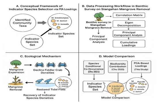
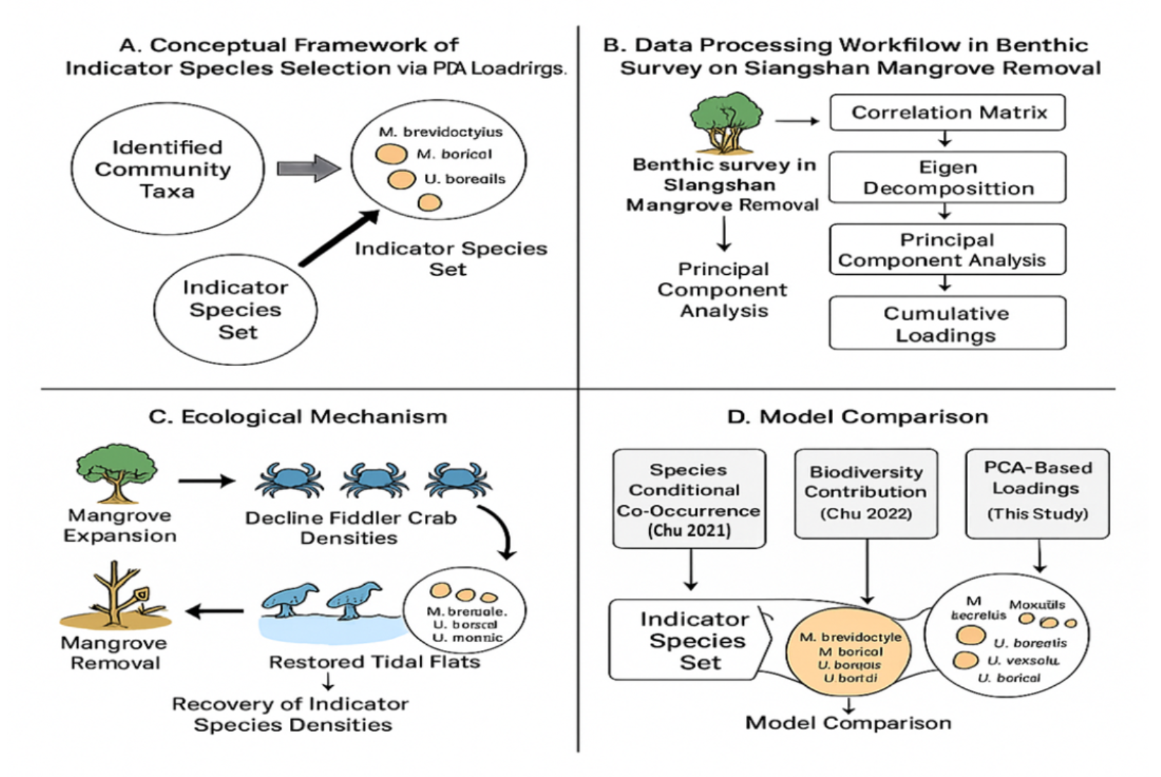
Graphical Abstract

1. Introduction

Mudflats are an important and unique type of wetland among coastal wetlands [1]. They consist of nutrient-rich fine silt and mud, forming a highly productive ecosystem that is vital to invertebrates, serving as their important foraging and breeding grounds, but is often threatened by development and construction [2]. Effective and low-cost monitoring is a crucial process for evaluating and assessing wetland management strategies. To understand these threats and changes, the application of biological indicators or indicator species (IS) as assessment tools has been widely used to evaluate environmental impacts such as bioindicators or indicator species (IS) [3,4,5,6,7,8]. Interpreting species signals is crucial because they reflect the emergence of early warning indicators and the occurrence of stressors [9]. Most ISs are single species or a few target species, using specific characteristics as proxy or paradigmatic to represent community indicators [9]. Therefore, ISs are also called umbrella species [10,11], keystone species [12,13,14], flagship species [10,12,13], or foundation species [14], depending on their ecological characteristics. These species are easy to monitor and their status can reflect or predict the status of their environment [8,15,16,17,18]. In other words, indicator organisms may be used as surrogates for a specific group of organisms to monitor the status of a specific environment, ecosystem, region, or habitat. Beyond pollution monitoring, indicator species serve multiple purposes including assessment of habitat disruption or continuity, ecosystem succession, and recovery from disturbance. Indicator species are typically selected based on their sensitivity to environmental changes or stressors such as pollution, eutrophication, or habitat alteration. Traditional selection methods often rely on expert judgment, single-species abundance thresholds, or correlation with known environmental gradients. However, these approaches may not adequately capture the multivariate nature of species assemblages responding to complex environmental change. Multivariate statistical methods, particularly ordination techniques, offer potential advantages for indicator species selection by simultaneously considering multiple species and their covariation patterns. Principal component analysis (PCA), while widely used in ecology for exploring community structure, has not been extensively applied as a quantitative framework for systematically identifying indicator species based on their contribution to community variation.
They are usually selected based on their sensitivity to environmental changes or stressors such as pollution, eutrophication, or habitat alteration [17]. Also, they help us to understand the health of ecosystems and help monitor the impacts of human activities. For example, marine organisms such as diatoms, polychaetes, and certain fish have been widely studied for their potential as indicators for monitoring water quality, pollution, and ecosystem stress [19,20]. The concept of indicator species is generally defined as one (or a few) species that can reflect the state of their environment or specific ecological conditions and serve as a proxy for the broader community or overall biodiversity in a given area [21,22]. In other words, the presence or absence of a particular species can reflect the state of environmental change and the integrity of the ecosystem [23]. Furthermore, ISs are used in a wide range of settings, including watersheds [24], lakes [25,26], semi-natural pastures [27,28], grasslands [29], and forests [30]. For example, polychaetes (Annelids) have been used as ecosystem indicators of marine pollution [31], using ISs to assess the state of macrobenthic communities [32], and Brachyuran crabs as a biomonitoring tool [33]. Specific traits of ecosystem function are also used to assess the role of organisms in ecosystem processes. These traits include migration capacity, reproductive strategy, and trophic level [34,35].
Several studies have used statistical methods to screen for ISs. For example, based on the probability of species appearing in different times and spaces, these candidate species can be identified by the cumulative maximum co-occurrence probability algorithm [36]. Similarly, these organisms were identified by studying species co-occurrence association patterns [37]. In this study, a mangrove removal program restored benthic habitats using a species conditional co-occurrence model, improved biodiversity indicators, and highlighted species such as Mictyris brevidactylus as effective ISs [37]. Co-occurrence analysis can predict species recovery under threat management and emphasize the importance of network connectivity between species [38]. This approach allows the development of community-wide response models based on limited species data [38]. However, when using the calculated joint probability, it is not possible to distinguish such relationships between species. This case study focuses on benthic crab species as indicators. Another study has used the species-in-biodiversity relationship approach to screen ISs [39].
This study employs principal component analysis (PCA) to address this problem. In addition to using common software for analysis, we developed a separate programming language for computation, allowing for a combined approach to understanding the calculation process. First, we calculated the correlation probability between each species and other species. Secondly, the component loading of PCA is accumulated on each species, and the probability of each species on each component is projected. Third, we selected the species with the highest cumulative load probability of all components and the species with higher individual component load as indicator species. Fourth, this case study uses data from the mangrove removal plan in Siangsan Wetland, Hsinchu, Taiwan. Finally, we explore a new quantitative approach to selecting indicator species based on PCA. PCA has been extensively applied in environmental monitoring [40,41,42,43,44], microbial community analysis [45,46,47,48,49], and pollution assessment [50,51,52].
Several studies have demonstrated PCA’s utility in revealing species–environment relationships and identifying species contributing most to community variation [53,54,55]. However, these studies have not formalized PCA as a systematic tool for indicator species selection with explicit quantitative criteria [56,57,58,59]. This study addresses this gap by developing a PCA-based framework that uses component loading scores to objectively identify indicator species. The primary objective of this study is to establish a robust quantitative framework for identifying indicator species utilizing principal component analysis (PCA). Specifically, this research seeks to identify key taxa capable of effectively monitoring environmental transitions following mangrove removal, with subsequent validation conducted through a rigorous analysis of their temporal and spatial distributions.
It is hypothesized that species exhibiting the highest cumulative component loading scores across all principal components serve as the most reliable indicators for tracking environmental shifts (H1). Furthermore, it is anticipated that these selected indicators will demonstrate significant, measurable responses to habitat modifications resulting from mangrove clearance (H2). Finally, this study proposes that a PCA-based selection methodology will yield results consistent with established ecological assessment techniques, including co-occurrence probability and biodiversity contribution metrics (H3), thereby providing a streamlined yet scientifically rigorous approach to ecosystem monitoring. The species with the highest cumulative load probability across all components and the species with higher individual component loads were selected as indicator species.

2. Materials and Methods

2.1. Case Study and Background

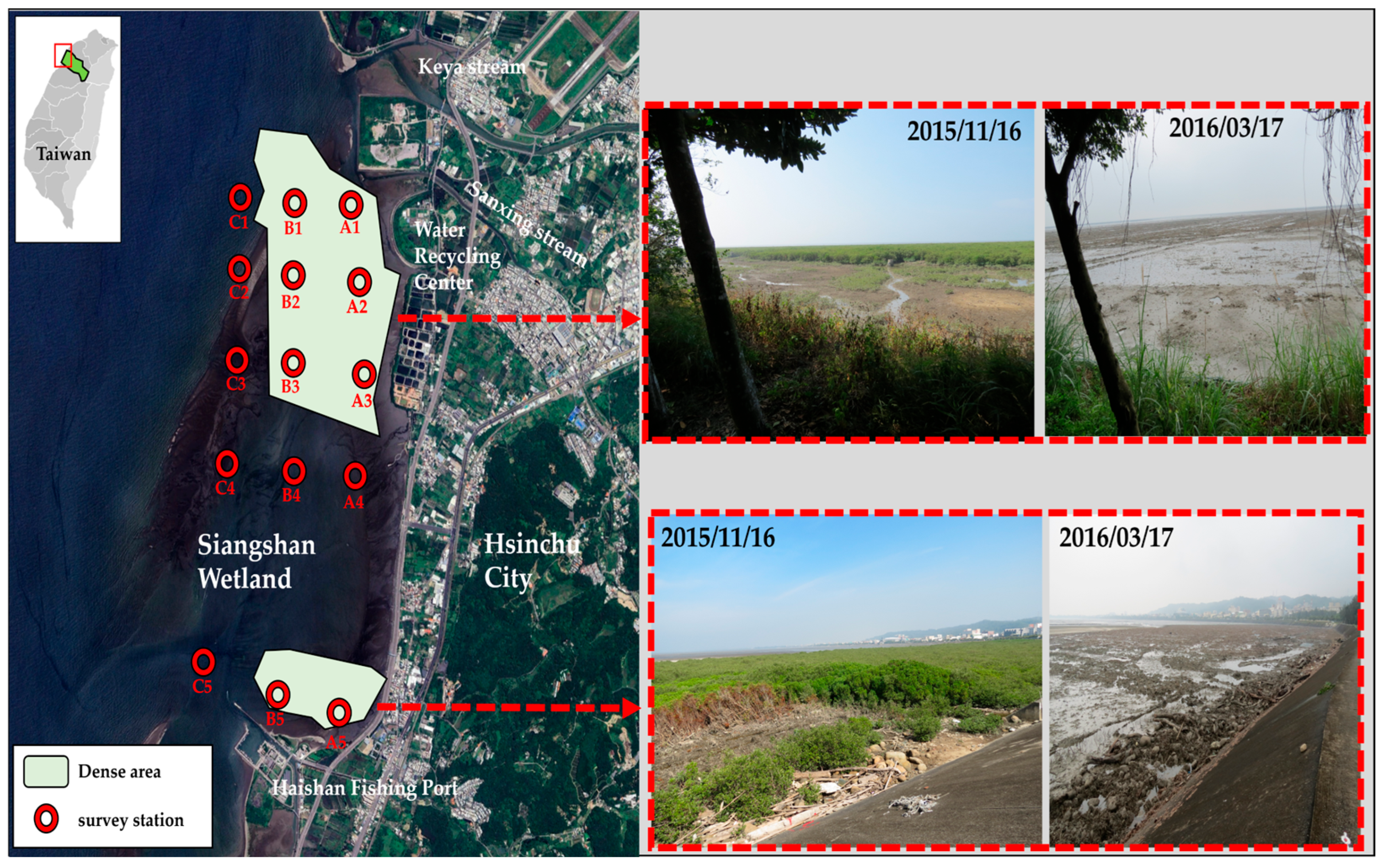
Siangshan Wetland is located on the coast of Hsinchu City, Taiwan. Its coastal wetland stretches 15 km from near Jincheng Lake in the north to Haishan Fishing Port in the south, covering an area of approximately 1700 hectares [60]. The area was originally planned to be filled in for land reclamation, but this was canceled after long-term protests and opposition from the conservation community. In 2001, it was designated as an important habitat for wildlife in Siangshan Wetland and a coastal wildlife reserve in Hsinchu City, covering 1600 hectares. It was formed by the erosion of the Touqian River, Niupu River, and Yanshui River. From north to south, it consists of the Keya River Estuary Wetland, the Sanxinggong River and Dazhuang River Estuary Grassland Wetland, Siangshan Mudflat Wetland, Haishangu Mangrove Wetland, and Nangang Beach. The muddy intertidal zone is about 2 km long. The accumulated organic matter is the energy source for the detrital food web, nurturing a large number of shrimps, crabs, snails, and shellfish, and attracting a large number of waterbirds to forage and roost [61]. The environment and sampling sites of the study area are shown in Figure 1.
Mangroves have traditionally been valued for coastal conservation. However, Siangshan Wetland historically lacked mangroves until Kandelia candel was artificially introduced due to misunderstandings about ecosystem requirements. Following years of rapid expansion, the mangrove forest reached 107 hectares by 2000. This expansion caused multiple adverse impacts: substrate territorialization altered habitat characteristics, ecosystem changes reduced species abundance and biodiversity, and mosquito proliferation created public health concerns for local residents. In response to sustained resident protests regarding these impacts, the Hsinchu City Government initiated a mangrove removal project in 2011 following council review and approval. Although removal efforts proceeded between 2011 and 2015, implementation faced numerous challenges. In October 2015, the government approved large-scale mechanical removal, accompanied by ecological monitoring studies to assess habitat recovery in the removal areas [61,62].

2.2. Biological Survey

A benthic ecology study was approved to compare changes in the area before and after mangrove removal, conducted from October 2015 to September 2016. Considering the scope of the removal and the condition of the surrounding substrate, three survey transects—A, B, and C—were designed and investigated. A total of 15 sampling sites were installed across the three transects, with 5 sites per transect (Figure 1). To facilitate comparison with non-mangrove areas, eight locations within densely mangroved areas were specifically designated for intensive monitoring (A1, A2, A3, A5, B1, B2, B3, and B5). While all sites across three transects (A, B, and C) were surveyed for species composition, the eight designated sites in transects A and B received priority focus for temporal monitoring given their location within the mangrove removal zone. Transect C data (shown in Figure 1) are included to provide spatial context but represent reference conditions outside the primary removal area. The survey focused specifically on brachyuran crabs (Crustacea: Decapoda: Brachyura) as the target taxonomic group, given their abundance, ecological importance, and sensitivity to substrate and vegetation changes in mudflat wetlands. The biological survey data used in this case study were previously collected and reported by [39]. The current analysis represents a novel methodological approach (PCA-based indicator species selection) applied to these data to test and validate the proposed framework.
The survey method was to conduct a benthic organism survey in accordance with the “Standard Operating Procedures for Wetland Ecosystem Biodiversity Monitoring Systems” [63] and the “Technical Specifications for Marine Ecological Assessment” (EPA Announcement No. 0960058664A) [64].

2.3. PCA and Software Usage

To reveal the complex relationships and changes among different elements (species), Spearman correlation was employed in addition to PCA. It is one of the most commonly used multivariate analysis methods for exploring diverse elemental combinations. By reorganizing the data, relative elemental combinations can explain most of the information in the original dataset [56,57]. In this study, we used software such as R, SPSS 18, and Excel for data preprocessing, feature extraction, and component loading calculation. Comparison with our self-developed program showed consistent component loading scores. After completing this program, we further calculated the species weight values. PCA has been implemented in various software programs.

2.4. PCA Model Description and Programming

PCA involves linear combinations of the original variables used to explain the variance in the data. This combination of elements makes the original data easier to visualize and allows for the derivation of meaningful patterns of elements among biological species. Below, we describe the PCA calculation process, except that we use software and write our own programming language. All PCA analyses were performed using R version 4.0.3 (R Core Team, 2020), SPSS version 26.0 (IBM Corp., Armonk, NY, USA), and Microsoft Excel 2019 for data preprocessing, feature extraction, and component loading calculation. To verify computational accuracy and enhance transparency, we additionally developed a custom Python script to perform PCA calculations independently, confirming consistency with commercial software outputs. For a dataset X, x is the variable, and k is the number of variables (i.e., the number of species). PCA is used to transform n observed variables into k principal component variables (Equation (1)):
f 1 = a 11 x 1 + a 21 x 2 + + a n 1 x n
f k = a 1 k x 1 + a 2 k x 2 + + a n k x n
f1 is defined as the first principal component, f2 is defined as the second principal component, and … fk is defined as the kth principal component. The maximum number of components extracted always equals the number of variables. The eigenvectors, which comprise coefficients corresponding to each variable, are used to calculate the principal component scores. The coefficients indicate the relative weight of each variable in the component. aij is defined as the principal component coefficient, which describes the correlation coefficient between the new variable fi and the original variable xj. The larger the aij value, the greater the correlation between fi and xj. PCA is performed by singular value decomposition of the matrix X [58,59].
ISs are defined as those whose presence denotes a major contribution to species correlation. That is, the presence and abundance of certain species contribute high index values. ISs should occur in a specific habitat, community or ecosystem composition and make a significant contribution to the relatedness of species to each other. Therefore, we formalized the calculation of survey data of species to establish a quantitative method for determining ISs. The respective equations for this index are as shown in Equation (2):
F = w 1 f 1 + w 2 f 2 + + w k f k
where f1, f2, …, fk are k principal components that describe the original variables.

2.4.1. Calculate the Correlation Matrix (R)

Spearman’s coefficient (rs) was additionally employed to comprehensively assess species relationships because ecological count data often violate normality assumptions and contain outliers. This non-parametric approach provides robustness against non-normal distributions and outliers commonly encountered in field surveys.
Prior to analysis, we tested our data for normality using the Shapiro–Wilk test, which indicated significant deviations from normality for several species (p < 0.05). Therefore, presented herein are results from one method to ensure robust conclusions. The first step is to calculate the correlation coefficient between species. The correlation coefficient matrix is a symmetric matrix, and the elements in the matrix are the correlation coefficients between two variables. In this study, the Spearman coefficient is used to obtain the correlation matrix R, the formula of which is shown below.
R = ( r i j ) n × n = r 11 r 12 r 1 n r 21 r 22 r 2 n r n 1 r n 2 r n n

2.4.2. Calculate Eigenvalues and Eigenvectors

Since the correlation matrix R is a real symmetric matrix and its eigenvalues (λj) are real numbers, eigenvalues can be obtained by solving the characteristic equation Det(RλE). The formula is as follows by solving the characteristic equation (Equation (3)):
R λ E = 0
The eigenvector (αj) can be obtained from the eigenvalue obtained above, via (RλE) α = 0, and has a non-zero solution. The solution vector corresponding to λ is called its eigenvector. Sometimes it can also be called the eigenvector of the matrix R, so the formula can be converted as follows via Equation (4):
r 11 λ j r 12 r 1 n r 21 r 22 λ j r 2 n r n i r n 2 r n n λ j α 1 j α 2 j α n j = 0
The eigenvector αj corresponding to the eigenvalue λj can be obtained from the following equation:
α j = ( α 1 j , α 2 j , , α n j ) T

2.4.3. Component Extraction

The important task is to extract k < m principal components. This enables appropriate representation of m variables with a small number of k principal components. The fewer components extracted, the better, and the larger the variation in each variable that the extracted components can explain, the better. Therefore, when extracting principal components, if the cumulative contribution rate of the extracted components exceeds a certain proportion or limits the number and size of eigenvalues, such as components with a cumulative contribution rate > 85% or eigenvalues > 1, before extracting common factors, the contribution rate and its cumulative contribution rate must be calculated first. The calculation method is as follows:
t i = λ j i = 1 n λ j
where ti is the contribution rate of the i-th principal component.
T i = λ 1 + λ 2 + + λ n i = 1 n λ j
where Ti is the cumulative contribution rate of the i-th principal component.
k principal components fi (i = 1, 2, …, k) can be extracted from the above formula, and the principal components fi can be expressed as shown in Equation (5):
f 1 = g 11 X 1 + g 21 X 2 + + g n 1 X n f 2 = g 12 X 1 + g 22 X 2 + + g n 2 X n f k = g 1 k X 1 + g 2 k X 2 + + g n k X n
where Xi (i = 1, 2, …, n) is the indicator variable used; gij (i = 1, 2, …, n; j = 1, 2, …, k) is the component loading. The component loading matrix is calculated as Equation (6):
g i j = α 11 λ 1 α 12 λ 2 α 1 k λ k α 21 λ 1 α 22 λ 2 α 2 k λ k α n 1 λ 1 α n 2 λ 2 α n k λ k = g 11 g 12 g 1 k g 21 g 22 g 2 k g n 1 g n 2 g n k
Component loadings are used as weight values. However, since factor loading values can be positive or negative, this is contrary to the assumption that the weight expected in this study must be greater than zero. Therefore, squaring the factor loadings eliminates problems with negative values. So, Equation (5) can be modified into Equation (7).
f 1 = h 11 2 X 1 + h 21 2 X 2 + + h n 1 2 X n f 2 = h 12 2 X 1 + h 22 2 X 2 + + h n 2 2 X n f k = h 1 k 2 X 1 + h 2 k 2 X 2 + + h n k 2 X n

2.4.4. Weight Calculation

To understand the contribution of ISs to all principal component loadings, we summed the loading scores for each species using Equation (8), which represents the contribution of all principal components in total. The calculation method is as follows:
F = ( w 1 h 11 2 + w 2 h 12 2 + + w k h 1 k 2 ) X 1 + ( w 1 h 21 2 + w 2 h 22 2 + + w k h 2 k 2 ) X 2 + + ( w 1 h n 1 2 + w 2 h n 2 2 + + w k h n k 2 ) X n = j = 1 k ( w j h 1 j 2 ) X 1 + j = 1 k ( w j h 2 j 2 ) X 2 + + j = 1 k ( w j h n j 2 ) X n
At this time, the weight of each IS can be converted into the expression of Equation (9).
W i = j = 1 k ( w j h i j 2 )

2.4.5. Identify ISs

To determine ISs, the species with the largest weight value among all species can be selected, that is, the maximum value of the cumulative load scores of all principal components, as shown in Equation (10).
m a x   W i X i

3. Results

3.1. Correlation Patterns Among Species (Supporting Objective 1)

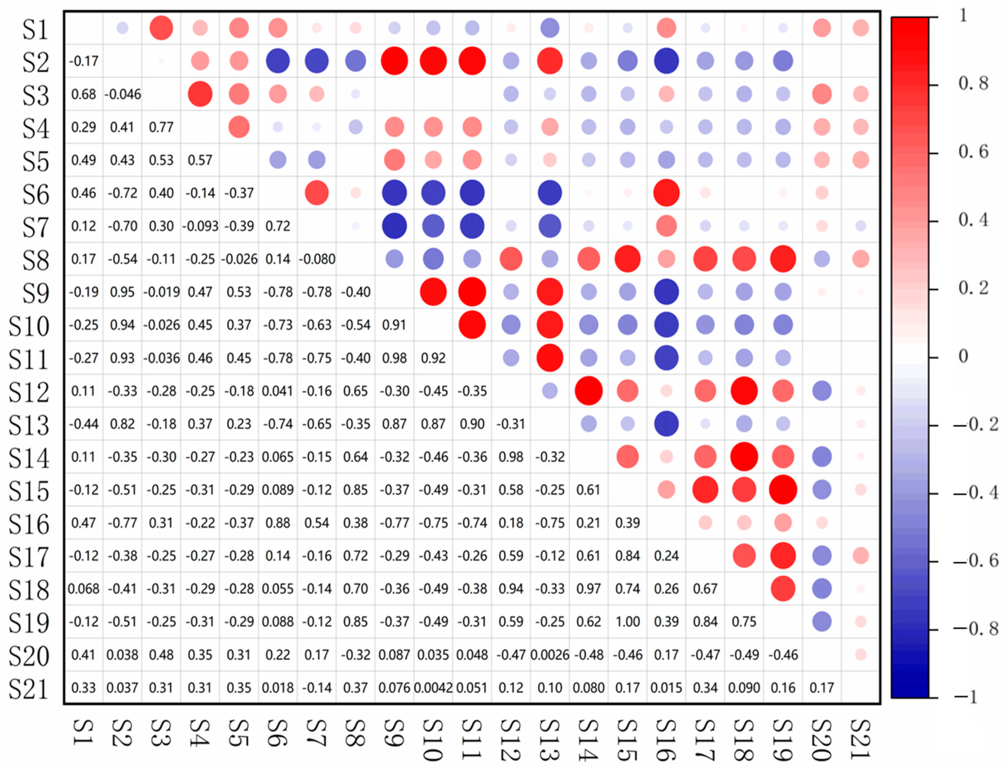
Spearman correlation analysis showed that among the 21 species in Siangsan Wetland (Figure 2), 18 of the 210 species pairings showed a high positive correlation (rs ≥ 0.75), accounting for 8.6% of the total number of species pairings. In addition, 13 species pairs showed good correlation (0.50 ≤ rs < 0.75), accounting for 6.2% of the total. Twenty-seven species pairs showed low correlation (0.25 ≤ rs < 0.50), accounting for 12.9% of the total. Thirteen species showed strong negative correlations (−0.75 ≤ rs), accounting for 6.2% of the total. Nineteen species pairs exhibited negative correlation (−0.50 ≤ rs < −0.75), which accounted for 9.1% of the total.

3.2. Principal Component Loadings (Supporting Objective 1)

The primary analysis utilizes Spearman’s correlation, given its prevalence in ecological PCA as a robustness check. This supplementary validation confirms that the observed trends remain consistent across different statistical assumptions.
Similarly, the other set of principal component loads is calculated based on Spearman coefficients. In this part, we used a self-written program to calculate the component loading score. After completing this program, we further calculated the species weight value. Based on the criterion that the eigenvalue is greater than 1, four principal components were also selected. The four main components of each crab species and their loading values are listed in Table 1. In the first principal component axis, H. formosensis, U. arcuata, U. formosensi, U. lacteal, and U. borealis were the major contributing species. In the second principal component axis, Uca perplexa, S. longidactyla, S. globosa, S. serrata, P. dubius, and D. penicillatus were the major contributing species. In the third principal component axis, H. doerjesi, M. brevidactylus, M. banzai, M. reviatus, and P. obtusifrons were the major contributing species. In the fourth principal component axis, no species was the main contributing species.

3.3. Selection of Indicator Species (Addressing Objectives 1 and 2)

In addition to the above-mentioned species with high loading scores in each principal component that can be used as indicator species, we also further calculated the total loading score for comparison. Through the calculation of Spearman correlation matrix, the weight and ranking of each species are shown in Table 2. The top five species are U. arcuata, U. formosensi, H. formosensis, U. lacteal, and U. borealis. Comparing the weights and rankings through the Spearman correlation matrix, there are some slight differences between the two, but the trend is consistent. The top five selected indicator species are the same but the ordering is slightly different.

3.4. Validation Through Monitoring (Addressing Objectives 2 and 3, Testing Hypothesis H2)

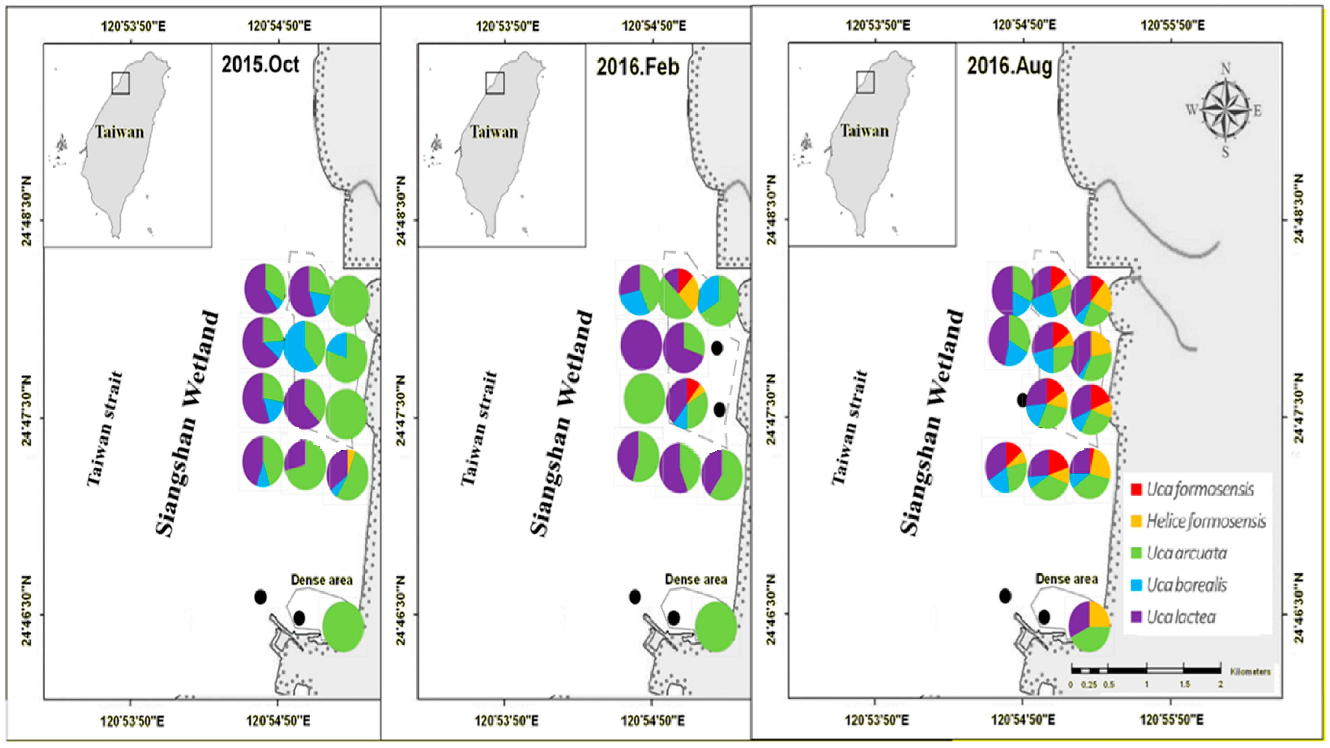
The spatial variations in ISs and other species composition are shown in Figure 2. The figure shows three different time periods before (October 2015) and after (August 2016) the removal of mangroves. Prior to the removal of the mangroves, four crab species were observed at sampling sites at the edge of the mangrove area: U. formosensis, U. arcuata, U. borealis, and U. lacteal. The spatial distribution of species composition in October 2015 and February 2016 showed that there were very few species in the mangrove area (Figure 3). These four species were also observed in the area after the mangroves were removed during the project. Clearly, the species composition in August 2016 showed a higher number of species. This suggests that the nature of the habitat has been altered and the species composition changed after the mangroves were removed.
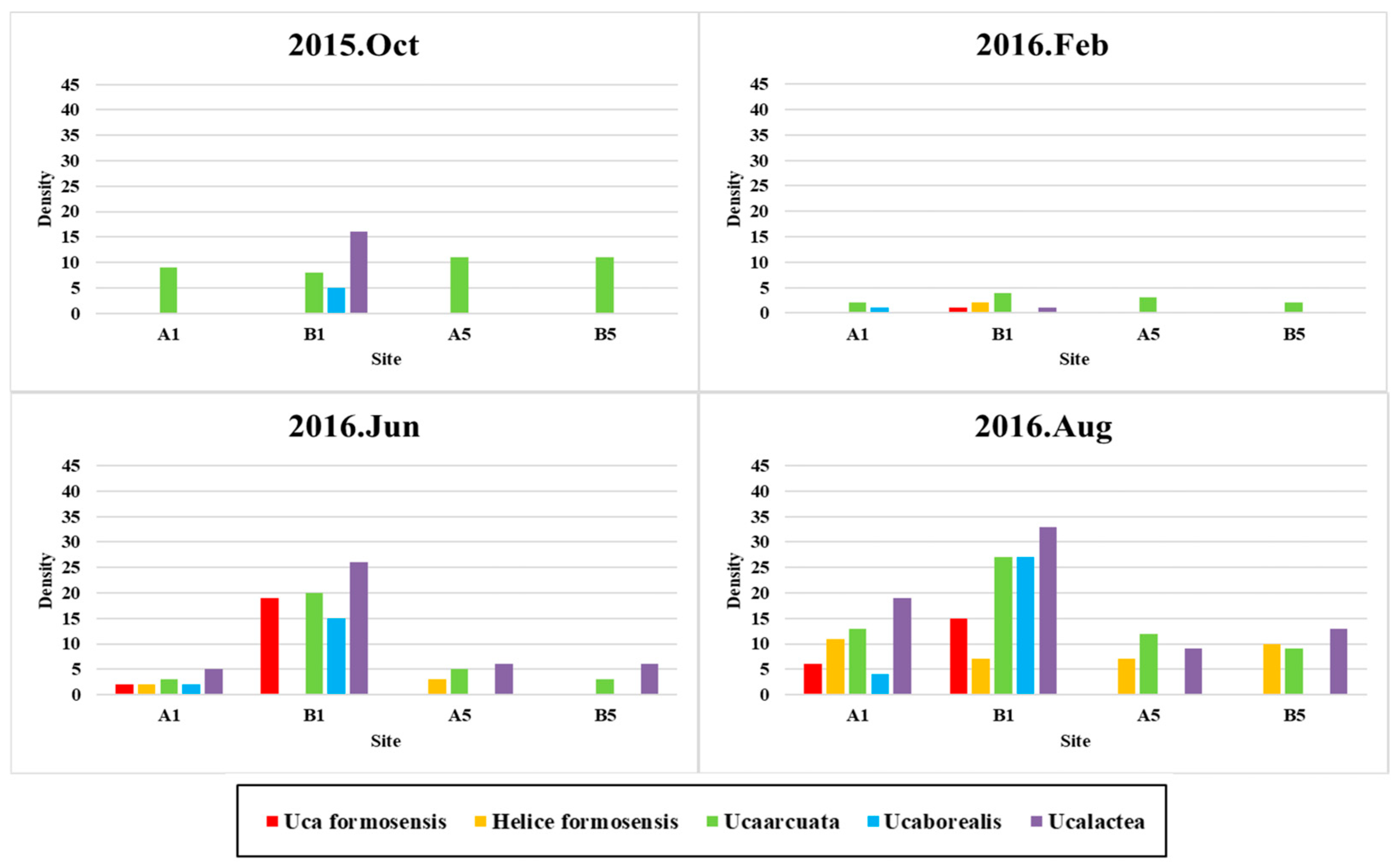
In this study, there were two different habitat types at the monitoring sites, namely mangroves (A1, A5) and non-mangroves (B1, B5). We compared the densities of five ISs (Figure 4). The density of crab species changes over time, and the density measured in mangrove areas is significantly lower than that in non-mangrove areas. After the mangroves were removed, these species moved into the area and their densities gradually returned to their original levels.

4. Discussion

4.1. Comparison with Previous Research

This study employed PCA-based component loadings to identify indicator species, while our previous research utilized species co-occurrence conditional probability [37] and biodiversity contribution methods [39]. While all three approaches identified similar indicator species (Table 3), critical evaluation reveals distinct methodological strengths, limitations, and appropriate application contexts for each framework. The PCA-based method offers several compelling advantages for indicator species selection. First, it provides fully quantitative, objective criteria based on statistical variance decomposition, eliminating subjective threshold selection that can introduce researcher bias. The loading scores represent mathematically defined contributions to community variation, making the selection process transparent and reproducible across different analysts and study systems. Second, PCA simultaneously captures multiple environmental gradients through orthogonal principal components, revealing species responses to independent axes of variation. This multivariate perspective is particularly valuable in complex ecosystems where environmental change operates along multiple dimensions simultaneously. Third, the method requires no a priori ecological assumptions about species relationships, umbrella effects, or biodiversity targets. This assumption-free characteristic makes PCA applicable even in poorly studied systems where ecological knowledge is limited. Fourth, PCA is computationally accessible, is implemented in standard statistical software (R, SPSS 18, Python), and does not require specialized programming expertise, facilitating adoption by resource managers and practitioners. Finally, the component structure itself provides interpretable ecological information about the environmental gradients structuring the community, offering mechanistic insights beyond simple species identification.
Despite these advantages, the PCA method has several important limitations that must be acknowledged. First, PCA performance depends critically on sample size and data quality. Adequate representation of environmental gradients requires sufficient spatial and temporal replication; our dataset (21 species × 15 sites × 12 months = 3780 observations) provided reasonable power, but smaller surveys may yield unstable component structures. Second, PCA identifies species contributing to the dominant axes of variation but may overlook rare or specialized species responding to minor or orthogonal gradients. Species with low overall abundance but high indicator value for specific disturbances may receive low loadings if their signal is overwhelmed by dominant community patterns. Third, the method assumes linear relationships between species and environmental gradients. Non-linear responses (e.g., threshold effects, unimodal distributions along environmental gradients) may be inadequately captured, potentially requiring transformation or alternative ordination techniques such as Detrended Correspondence Analysis (DCA). Fourth, component interpretation can be ambiguous when multiple environmental factors co-vary, making it difficult to assign clear ecological meaning to extracted axes. In this study, PC1 clearly represented the mangrove removal gradient, but in systems with multiple simultaneous stressors, interpretation may be less straightforward. Fifth, PCA provides no direct assessment of whether selected indicators are practically monitorable or cost-effective; a species with high loadings may be cryptic, nocturnal, or otherwise difficult to survey in practice.
The co-occurrence probability approach [37] offers distinct advantages and limitations relative to PCA. Its primary strength lies in biological interpretability through the umbrella species concept—selected indicators are demonstrably associated with diverse co-occurring species, providing intuitive ecological justification. The method explicitly addresses practical monitoring concerns by prioritizing species that, when present, indicate the presence of multiple other species, potentially reducing survey effort. Furthermore, the probabilistic framework naturally handles sampling uncertainty and can incorporate detection probability, which PCA does not explicitly address. However, the co-occurrence method has notable weaknesses. The selection of probability thresholds (e.g., P > 0.7 for “strong” co-occurrence) is somewhat arbitrary and can significantly influence which species are identified as indicators. The method assumes that co-occurrence patterns reflect causal ecological relationships (e.g., shared habitat requirements), but species may co-occur coincidentally without functional association. Additionally, the approach is computationally intensive for large species pools, requiring pairwise conditional probability calculations for all possible species combinations (for 21 species: 210 pairwise comparisons). Most critically, the method does not explicitly quantify how much of the community variation each indicator captures, making it difficult to assess whether selected species adequately represent ecosystem change.
The biodiversity contribution framework [39] aligns directly with conservation objectives by prioritizing species that most enhance alpha or beta diversity indices (e.g., Shannon diversity, Simpson’s index). This target-oriented approach has strong appeal when biodiversity maintenance is the explicit management goal, as in many protected area contexts. The method also naturally incorporates both abundance and richness information, potentially identifying indicators that reflect both common and rare species. However, this approach has several limitations. It assumes biodiversity itself is the appropriate management target, which may not hold when specific ecosystem functions or services are prioritized (e.g., carbon sequestration, fishery production). The method is sensitive to the choice of diversity index, and different indices (Shannon, Simpson, taxonomic diversity) may identify different indicators. Furthermore, species contributing most to biodiversity may not necessarily respond most sensitively to the environmental change of interest—a highly diverse community may change in composition without changing in overall diversity. In our case, while the method successfully identified species sensitive to mangrove removal, this outcome is not guaranteed in all contexts. Finally, like the co-occurrence method, the biodiversity contribution approach does not reveal the environmental gradients to which indicators respond, limiting mechanistic understanding. Based on our comparative analysis, we propose the following decision framework for indicator species selection: Use PCA when (1) comprehensive multivariate data exist across environmental gradients; (2) multiple simultaneous environmental changes require separation; (3) objective, reproducible criteria are prioritized; (4) mechanistic understanding of species–environment relationships is desired; (5) the study system is poorly known with limited a priori ecological knowledge. Use co-occurrence probability when (1) monitoring efficiency is paramount and surveying indicator species should predict the presence of many other species; (2) umbrella species concepts align with conservation goals; (3) the community structure reflects strong species associations; (4) practical field implementation requires biologically intuitive indicators. Use biodiversity contribution when (1) biodiversity conservation is the explicit management objective; (2) both common and rare species must be considered; (3) diversity indices are established monitoring metrics; (4) the goal is to track community-level changes rather than specific environmental factors. Use multiple methods when resources permit and convergent validity across approaches strengthens confidence in selected indicators, as demonstrated in this study where five species consistently emerged across all three methods.
Our PCA approach offers several advantages: it is fully quantitative and reproducible, requires no a priori assumptions about species relationships, and is computationally accessible. However, it requires substantial multivariate data and may be less effective when key indicator species are rare or have unique environmental requirements not captured by the dominant gradients. The co-occurrence method [37] offers biological interpretability (umbrella species concept) but depends on probability thresholds that may be somewhat arbitrary. The biodiversity contribution method [39] has strong conservation relevance but assumes biodiversity itself is the management target. For wetland restoration monitoring, we recommend using PCA when (1) adequate survey data exist across environmental gradients, (2) multiple species respond to the management action, and (3) objective, reproducible selection criteria are required. The method is particularly valuable for establishing baseline monitoring protocols where expert knowledge may be limited.
A critical challenge in comparing these methods is that “accuracy” in indicator species selection cannot be objectively quantified in the absence of ground truth. Unlike predictive models where accuracy metrics (e.g., AUC, RMSE) can be calculated against known outcomes, indicator selection requires validation against multiple subjective criteria: ecological sensitivity, monitoring feasibility, cost-effectiveness, and stakeholder acceptance. This study demonstrates convergent validity—different methods yield similar results—which provides confidence but does not prove that selected species are “correct” indicators. Proper validation of indicator species requires demonstrating that (1) indicators respond measurably and predictably to the target environmental change (supported by our temporal data, Figure 4); (2) indicators provide early warning before community-wide impacts occur (not tested in this study); (3) indicator responses are consistent across spatial replicates (partially supported by our transect comparisons); (4) monitoring indicators is more cost-effective than surveying the entire community (economic analysis beyond our scope). Future research should explicitly test these validation criteria across multiple study systems and environmental contexts.
Our comparative evaluation has important limitations. All three methods were applied to the same dataset from a single wetland system, limiting generalizability. The methods may perform differently in systems with distinct community structures, environmental gradients, or monitoring objectives. Additionally, we compared methods retrospectively on existing data; a prospective study establishing monitoring protocols based on each method and tracking long-term outcomes would provide more definitive comparative evidence. Finally, our evaluation focused on ecological and statistical criteria but did not assess practical implementation considerations such as field time requirements, taxonomic expertise needed, or cost differentials—factors that often determine method adoption in real-world management contexts.

4.2. Understanding of PCA Application

In multivariate data analysis, PCA is a widely used tool that can reduce data dimensionality while preserving data variability as much as possible [64,65]. In other words, it is a method that converts multiple variables into a few indicators while maintaining the maximum correlation with the original data. The importance of a species can be measured by the cumulative load score of each component. Therefore, a corresponding species importance assessment model can be established with the relative weight Wi as the coefficient. In some past studies, complex ecological and environmental datasets were simplified to the most informative components using PCA [65,66,67,68,69]. For example, ref. [69] used PCA to reduce 72 environmental indicators to a manageable set of effective dimensions for monitoring, while [70] applied PCA to identify which indicator organisms most effectively reflected PAH pollution patterns across multiple sites and species. Its applications include environmental monitoring [66], microbial community analysis [65], and health-related biomarker discovery, and it has shown its practicality in various research fields. The presence of certain pollutants or ecological conditions can be inferred from the interaction of organisms with the environment. In this study, we adopted this concept and developed a corresponding species importance assessment model.
In this study, four principal components were selected based on the calculation of the Spearman correlation coefficient and the eigenvalue being greater than 1 (Table 1). The four principal components and their factor loadings for each crab species are also listed. A higher loading value for each principal component indicates a greater contribution of that variable to that component. In the first principal component axis, H. formosensis, M. brevidactylus, M. banzai, U. arcuata, U. formosensi, U. lacteal, and U. borealis were the major contributing species throughout the entire period. In the second principal component axis, O. sinensis, U. perplexa, S. longidactyla, S. globosa, S. serrata, P. dubius, and D. penicillatus were the major contributing species. In the third principal component axis, H. doerjesi, M. reviatus, and O. ceratophthalmus were the major contributing species. In the fourth principal component axis, S. bitympana was the main contributing species.
The principal component loadings reveal distinct ecological gradients that structure the benthic crab community in response to mangrove removal [71,72]. Each principal component represents a different axis of environmental variation, with species loadings reflecting their sensitivity and response to these underlying gradients. The first principal component (PC1, explaining 41.2% of variance) appears to represent a gradient of habitat openness and substrate exposure. Species exhibiting high positive loadings on PC1—U. formosensis, U. arcuata, U. lactea, and U. borealis—are obligate mudflat specialists that require exposed, well-oxygenated substrates for burrow construction and foraging. These fiddler crab species are typically excluded from densely vegetated mangrove areas due to root structure interference, reduced light penetration, and substrate anoxia. Their high loadings on PC1 indicate strong positive responses to mangrove removal, which restores the open mudflat conditions essential for their survival. The ecological significance of PC1 thus reflects the primary environmental impact of the management intervention: the transition from terrestrialized, vegetated habitat to open intertidal mudflat. The second principal component (PC2, explaining 36.3% of variance) captures variation along a substrate texture gradient, distinguishing sandy from muddy habitats. High-loading species on PC2 include O. sinensis, S. longidactyla, and S. globosa, which are characteristically associated with sandy or mixed sand–mud substrates. These species possess morphological and behavioral adaptations for sand-dominated environments, including specialized setae for particle manipulation and rapid burrowing capabilities. The emergence of PC2 as a significant axis suggests that mangrove removal not only affects vegetation structure but also influences substrate heterogeneity, potentially through altered sedimentation patterns and hydrodynamic regimes. The moderate loadings of several species on PC2 indicate that the wetland encompasses a mosaic of substrate types, with some areas developing sandier conditions post-removal.
The third principal component (PC3, explaining 7.4% of variance) reflects variation related to tidal elevation and estuarine influence. H. doerjesi, M. abbreviatus, and O. ceratophthalmus show high loadings on PC3, representing species assemblages characteristic of mid-tidal zones with significant freshwater input. H. doerjesi, in particular, exhibits eurytopic tendencies, tolerating a wide range of salinity and substrate conditions commonly found in estuarine transitional zones. The relatively low variance explained by PC3 suggests that tidal elevation effects are secondary to the primary habitat transformation (PC1) and substrate composition (PC2) in structuring the community during the recovery period. Critically, the dominance of PC1 and the high loadings of mudflat specialists on this axis provide quantitative evidence that mangrove removal successfully restored habitat conditions favorable to native mudflat fauna. The co-occurrence of multiple fiddler crab species with high PC1 loadings suggests functional redundancy in response to habitat opening, which may confer resilience to the restored community. Furthermore, the orthogonality of the principal components indicates that different species guilds respond to independent environmental gradients, supporting the selection of multiple indicator species to capture the multidimensional nature of ecosystem recovery. From a monitoring perspective, species with high loadings on PC1 serve as effective indicators of the primary management objective (habitat deterritorialization), while species loading on PC2 and PC3. This multi-axis interpretation demonstrates that PCA not only identifies indicator species but also reveals the mechanistic linkages between environmental change and community response, offering deeper ecological insight than univariate indicator selection methods. In terms of habitat, fiddler crabs prefer moist mud–sand environments. This explains why they may have inhabited wetland waterways and tidal pools after low tide. The expansion of mangroves led to the territorialization of the area, and the habitat substrate gradually became dry and solid. As mangroves expand, these species then migrate to areas at the edge of the mangroves. When the mangroves are removed, the substrate of the mangrove properties completely changes. When tidal channels and tide pools appear, the habitat properties change, and these species naturally return to their original habitats.
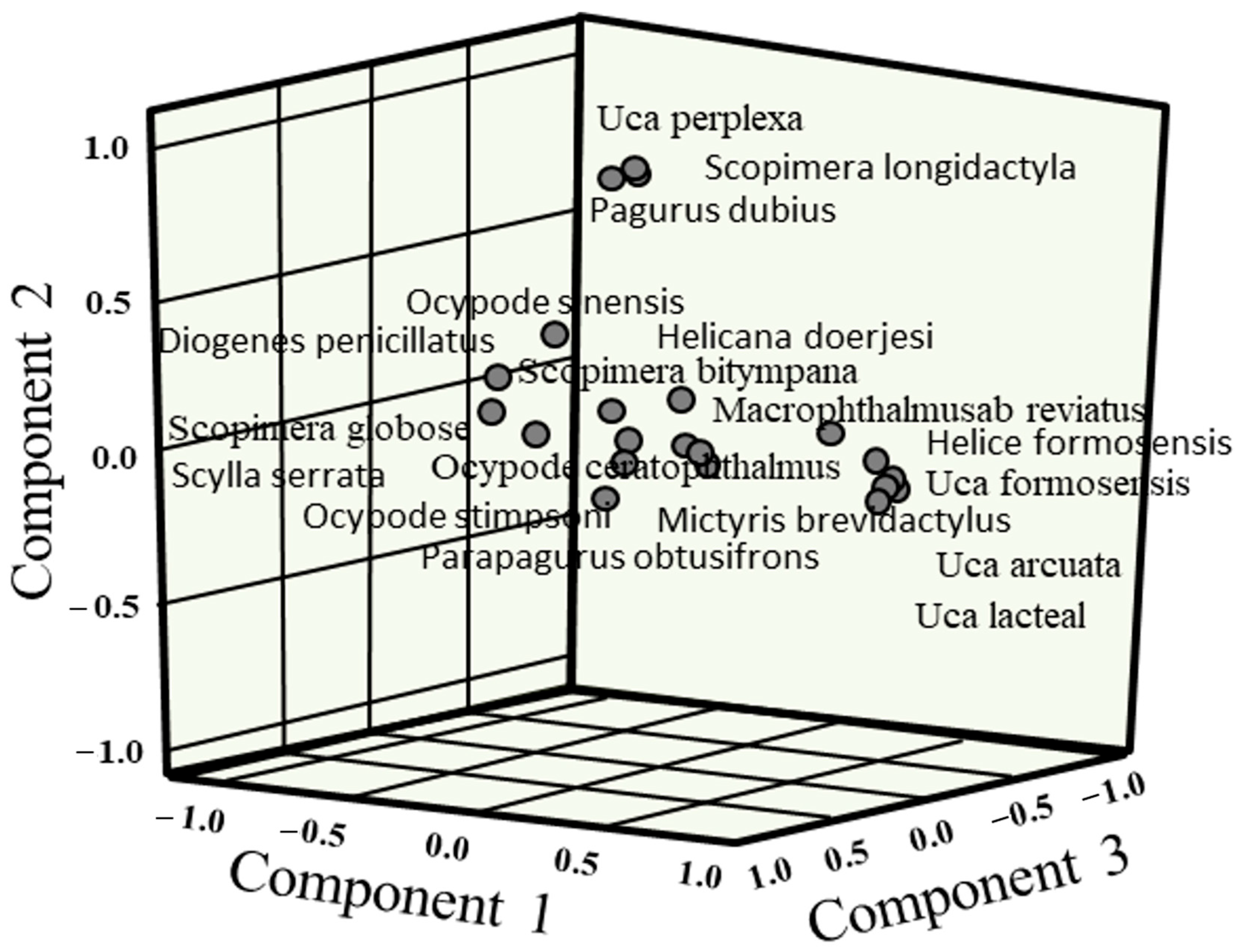
Furthermore, we plotted the three principal components in Figure 5, showing the relative locations of each species. For example, H. formosensis, U. formosensis, U. arcuate, U. lacteal, and U. borealis were observed at positions in the rightmost region of the first principal component. U. perplexa, S. longidactyla, and P. dubius were observed in the uppermost region of the second principal component. The diagram clearly shows that certain species are distinct in this 3D spatial map.
PCA effectively reveals the relative changes of organisms across principal components by highlighting patterns and trends. It helps to detect environmental anomalies and assess their trends [68]. PCA has been used to assess environmental indicators and has revealed significant redundancy in existing indicators. This has helped prioritize indicators related to air, water, biodiversity, and land, which are less abundant but have greater impact [69]. Application of PCA to coastal indicator organisms has shown that these organisms can effectively reflect polycyclic aromatic hydrocarbon (PAH) pollution in the environment, demonstrating their utility in long-term environmental monitoring [70]. Even with so many applied studies, there is still no approach similar to this study to select ISs. Using this approach to select ISs can expand the application scope of PCA, which is worth considering. While our previous studies [37,39] identified indicator species using co-occurrence probability and biodiversity contribution methods, neither approach provides a fully quantitative, mechanistic understanding of why particular species serve as effective indicators. This study addresses this gap by developing a PCA-based framework that explicitly links species selection to their contribution to community variance across multiple environmental gradients [73]. The novelty lies not in identifying which species are indicators, but in establishing a generalizable, reproducible methodology that can be applied to any multi-species dataset to systematically identify indicators based on statistical criteria rather than ecological assumptions.

4.3. Broader Implications, Limitations, and Future Research Directions

Our findings have broader implications beyond the Siangshan Wetland case study. The PCA-based indicator species selection approach could be applied to other mangrove restoration or removal projects globally, particularly where invasive mangrove species (e.g., Kandelia candel in Taiwan, Rhizophora spp. in Hawaii, Laguncularia racemosa in Brazil) have colonized non-native habitats. The method is particularly valuable for monitoring gradual ecosystem shifts where multiple species respond simultaneously to environmental change [74]. However, several limitations should be acknowledged. First, our approach requires substantial baseline data across multiple species and sampling periods. Second, the method identifies species that co-vary with dominant environmental gradients but may not capture species responding to subtle or orthogonal environmental factors. Third, our validation is based on a single wetland system over one year; longer-term and multi-site validation would strengthen confidence in the approach.
The convergence of results across three independent methods (co-occurrence, biodiversity contribution, and PCA loading scores) provides strong validation that the identified species are indeed robust indicators. However, the contribution of this study extends beyond confirming previous findings. We demonstrate that (1) PCA loading scores provide quantitative measures of each species’ contribution to community variation, enabling objective ranking and selection; (2) the principal component structure reveals different ecological guilds (tidal zone specialists, habitat generalists, etc.) that respond to different environmental gradients; (3) the method is fully transparent and reproducible, requiring no probability thresholds or biodiversity indices; (4) PCA can be implemented using standard statistical software, making it accessible to resource managers without specialized programming skills; (5) the component loadings provide interpretable ecological information about species–environment relationships. Most importantly, this study establishes PCA-based indicator selection as a generalizable framework that can be applied beyond the Siangshan Wetland case to other ecosystem monitoring contexts. Previous methods were developed specifically for this case study; the PCA framework offers broader applicability [73,74,75,76].
Future research should (1) test this method across different wetland types and geographic regions, (2) compare performance against other indicator selection approaches in varied ecological contexts, (3) develop criteria for determining adequate sample size and duration for robust PCA-based indicator selection, and (4) integrate this approach with trait-based ecology to understand why certain species emerge as effective indicators.

5. Conclusions

In conclusion, this study’s primary contribution is methodological: we demonstrate that PCA, a widely available statistical tool, can be formalized into a systematic framework for indicator species selection. The validation against previously identified indicators confirms the method’s reliability, while the computational transparency and accessibility enhance its potential for widespread application in ecosystem monitoring and conservation management. This study demonstrates the efficacy of a PCA-based methodological framework by successfully identifying five key indicator species—Mictyris brevidactylus, Macrophthalmus banzai, Uca arcuata, Uca lactea, and Uca borealis—thereby fulfilling the primary research objective and substantiating Hypothesis H1. The observed spatial and temporal distribution patterns of these species effectively tracked environmental shifts throughout the mangrove removal process, providing empirical support for Hypothesis H2 regarding their utility as sensitive ecological monitors. Furthermore, the consistent identification of these taxa across alternative frameworks—specifically species co-occurrence and biodiversity contribution methods—establishes robust convergent validity and confirms Hypothesis H3. Beyond its predictive power, the PCA approach is distinguished by its quantitative rigor, reproducibility, and accessibility within standard statistical software, offering the critical advantage of elucidating complex species–environment relationships through variance decomposition. Ultimately, these findings advocate for the broader implementation of PCA-based indicator selection in diverse restoration monitoring contexts and underscore the necessity of future research to validate the versatility and scalability of this framework across varied ecosystem types. While this study focused on mangrove removal monitoring, the PCA-based approach offers a generalizable framework for indicator species selection in diverse management contexts, including invasive species control, habitat restoration, and climate change monitoring. The method’s reliance on multivariate statistical relationships makes it particularly suited for complex ecosystems where multiple stressors and species interactions shape community dynamics.

Author Contributions

Conceptualization, Y.-Q.Z., T.-J.C., and C.-H.S.; methodology, T.-J.C., Y.-Q.Z., Y.-J.S., and C.-H.S.; software, Y.-Q.Z., T.-J.C., and Y.-J.S.; validation, C.-H.S., and Y.-Q.Z.; formal analysis, Y.-Q.Z., C.-H.S. and T.-J.C.; investigation, Y.-Q.Z., T.-J.C., C.-H.S., and Y.-J.S.; resources, Y.-Q.Z., T.-J.C. and C.-H.S.; data curation, Y.-Q.Z., T.-J.C. and C.-H.S.; writing—original draft preparation, T.-J.C. and C.-H.S.; writing—review and editing, T.-J.C., C.-H.S., and Y.-J.S.; visualization, T.-J.C., C.-H.S., Y.-J.S., and Y.-Q.Z.; supervision, T.-J.C. and C.-H.S.; project administration, T.-J.C. and C.-H.S.; funding acquisition, T.-J.C., Y.-J.S., and C.-H.S. All authors have read and agreed to the published version of the manuscript.

Funding

This work was supported by the Jimei University grant number C619061 and Taiwan Wetland Society grant number TWS 107-2221-A-002. The funders had no role in study design, data collection and analysis, the decision to publish, or the preparation of the manuscript.

Data Availability Statement

No new data were created or analyzed in this study. Data sharing is not applicable to this article.

Acknowledgments

We thank Kuo Yi-Yu for his contributions to the suggested revision comments to the manuscript. Useful suggestions from anonymous reviewers were incorporated into the manuscript.

Conflicts of Interest

The authors declare that there is no conflict of interest.

References

  1. Zuo, P.; Li, Y.; Liu, C.A.; Zhao, S.H.; Guan, D.M. Coastal wetlands of China: Changes from the 1970s to 2007 based on a new wetland classification system. Estuaries Coasts 2013, 36, 390–400. [Google Scholar] [CrossRef]
  2. Dissanayake, N.G.; Frid, C.L.J.; Drylie, T.P.; Caswell, B.A. Ecological functioning of mudflats: Global analysis reveals both regional differences and widespread conservation of functioning. Mar. Ecol. Prog. Ser. 2018, 604, 1–20. [Google Scholar] [CrossRef]
  3. Karr, J.R. Assessment of biotic integrity using fish communities. Fisheries 1981, 6, 21–27. [Google Scholar] [CrossRef]
  4. Whitfield, A.K.; Elliott, M. Fishes as indicators of environmental and ecological changes within estuaries: A review of progress and some suggestions for the future. J. Fish Biol. 2002, 61, 229–250. [Google Scholar] [CrossRef]
  5. Okwuosa, O.B.; Eyo, J.E.; Omovwohwovie, E.E. Role of fish as bioindicators: A review. Iconic Res. Eng. J. 2019, 2, 354–368. [Google Scholar]
  6. Belal, A.A.M. Macro-benthic invertebrates as a bio-indicator for water and sediment quality in Suez Bay, Red Sea. Egypt. J. Aquat. Res. 2019, 45, 123–130. [Google Scholar] [CrossRef]
  7. Kennedy, A.D.; Jacoby, C.A. Biological indicators of marine environmental health: Meiofauna—A neglected benthic component? Environ. Monit. Assess. 1999, 54, 47–68. [Google Scholar] [CrossRef]
  8. Azzazy, M.F. Plant bioindicators of pollution in Sadat City, Western Nile Delta, Egypt. PLoS ONE 2020, 15, e0226315. [Google Scholar] [CrossRef]
  9. Burant, J.B.; Park, C.; Betini, G.S.; Norris, D.R. Early warning indicators of population collapse in a seasonal environment. J. Anim. Ecol. 2021, 90, 1538–1549. [Google Scholar] [CrossRef]
  10. Caro, T. Surrogate Species in the Real World. In Conservation by Proxy: Indicator, Umbrella, Keystone, Flagship, and Other Surrogate Species; Caro, T., Girling, S., Eds.; Island Press: Washington, DC, USA, 2010; pp. 263–284. [Google Scholar]
  11. Menge, B.A.; Freidenburg, T.L.; Iles, A. Keystone species. In Encyclopedia of Biodiversity, 2nd ed.; Levin, S.A., Ed.; Academic Press: Cambridge, MA, USA, 2013; Volume 4, pp. 442–457. [Google Scholar]
  12. Deere, N.J.; Ramadiyanta, E.; Sibarani, M.C.; Hadi, A.N.; Andayani, N.; Ginting, Y.; Bull, J.W.; Struebig, M.J. Selecting umbrella species as mammal biodiversity indicators in tropical forest. Biol. Conserv. 2024, 292, 110511. [Google Scholar] [CrossRef]
  13. Gopal, B.; Junk, W.J. Biodiversity in wetlands: An introduction. In Biodiversity in Wetlands: Assessment, Function and Conservation; Gopal, B., Junk, W.J., Davis, J.A., Eds.; Backhuys: Leiden, The Netherlands, 2000; Volume 1, pp. 1–10. [Google Scholar]
  14. Cairns, J., Jr.; Pratt, J.R. A history of biological monitoring using benthic macroinvertebrates. In Freshwater Biomonitoring and Benthic Macroinvertebrates; Rosenberg, D.M., Resh, V.H., Eds.; Chapman & Hall: New York, NY, USA, 1993. [Google Scholar]
  15. Bartell, S.M. Biomarkers, bioindicators, and ecological risk assessment—A brief review and evaluation. Environ. Bioindic. 2006, 1, 39–52. [Google Scholar] [CrossRef]
  16. Burger, J. Bioindicators: Types, development, and use in ecological assessment and research. Environ. Bioindic. 2006, 1, 22–39. [Google Scholar] [CrossRef]
  17. Siddig, A.A.H.; Ellison, A.M.; Ochs, A.; Leeman, C.V.; Lau, M.K. How do ecologists select and use indicator species to monitor ecological change? Insights from 14 years of publication in Ecological Indicators. Ecol. Indic. 2016, 60, 223–230. [Google Scholar] [CrossRef]
  18. Lee, H.Y.; Shih, S.S. Impacts of vegetation changes on the hydraulic and sediment transport characteristics in Guandu mangrove wetland. Ecol. Eng. 2004, 23, 85–94. [Google Scholar] [CrossRef]
  19. Elliot, E.L.; Colwell, R.R. Indicator organisms for estuarine and marine waters. FEMS Microbiol. Rev. 1985, 1, 61–79. [Google Scholar] [CrossRef]
  20. Desrosiers, C.; Leflaive, J.; Eulin, A.; Ten-Hage, L. Bioindicators in marine waters: Benthic diatoms as a tool to assess water quality from eutrophic to oligotrophic coastal ecosystems. Ecol. Indic. 2013, 32, 25–34. [Google Scholar] [CrossRef]
  21. Lee, T.M.; Yeh, H.C. Applying remote sensing techniques to monitor shifting wetland vegetation: A case study of Danshui River estuary mangrove communities, Taiwan. Ecol. Eng. 2009, 35, 487–496. [Google Scholar] [CrossRef]
  22. Shih, S.S.; Yang, S.C.; Lee, H.Y.; Hwang, G.W.; Hsu, Y.M. Development of a salinity-secondary flow-approach model to predict mangrove spreading. Ecol. Eng. 2011, 37, 1174–1183. [Google Scholar] [CrossRef]
  23. Moyle, P.B.; Randall, P.J. Evaluating the biotic integrity of watersheds in the Sierra Nevada, California. Conserv. Biol. 1998, 12, 1318–1326. [Google Scholar] [CrossRef]
  24. Carignan, V.; Villard, M.A. Selecting indicator species to monitor ecological integrity: A review. Environ. Monit. Assess. 2002, 78, 45–61. [Google Scholar] [CrossRef]
  25. Harig, A.L.; Bain, M.B. Defining and restoring biological integrity in wilderness lakes. Ecol. Appl. 1998, 8, 71–87. [Google Scholar] [CrossRef]
  26. Pärt, T.; Söderström, B. Conservation value of semi-natural pastures in Sweden: Contrasting botanical and avian measures. Conserv. Biol. 1999, 13, 755–765. [Google Scholar] [CrossRef]
  27. Pärt, T.; Söderström, B. The effects of management regimes and location in landscape on the conservation of farmland birds in semi-natural pastures. Conserv. Biol. 1999, 90, 113–123. [Google Scholar] [CrossRef]
  28. Bradford, D.F.; Franson, S.E.; Neale, A.C.; Heggem, D.T.; Miller, G.R.; Canterbury, G.E. Bird species assemblages as indicators of biological integrity in Great Basin rangeland. Environ. Monit. Assess. 1998, 49, 1–22. [Google Scholar] [CrossRef]
  29. Brooks, R.P.; O’Connell, T.J.; Wardrop, D.H.; Jackson, L.E. Towards a regional index of biological integrity: The example of forested riparian ecosystems. Environ. Monit. Assess. 1998, 51, 131–143. [Google Scholar] [CrossRef]
  30. Dean, H.K. The use of polychaetes (Annelida) as indicator species of marine pollution: A review. Rev. Biol. Trop. 2008, 56, 11–38. [Google Scholar]
  31. Grizzle, R.E. Pollution indicator species of macrobenthos in a coastal lagoon. Mar. Ecol. Prog. Ser. 1984, 18, 191–200. [Google Scholar] [CrossRef]
  32. Bustos-Baez, S.; Frid, C. Using indicator species to assess the state of macrobenthic communities. Hydrobiologia 2003, 496, 299–309. [Google Scholar] [CrossRef]
  33. Arya, S.; Trivedi, J.N.; Vachhrajani, K.D. Brachyuran crabs as a biomonitoring tool: A conceptual framework for Chemical Pollution Assessment. Int. Res. J. Environ. 2014, 3, 49–57. [Google Scholar]
  34. Bremner, J. Species’ traits and ecological functioning in marine conservation and management. J. Exp. Mar. Biol. Ecol. 2008, 366, 37–47. [Google Scholar] [CrossRef]
  35. Costello, M.J.; Claus, S.; Dekeyzer, S.; Vandepitte, L.; Tuama, É.Ó.; Lear, D.; Tyler-Walters, H. Biological and ecological traits of marine species. PeerJ 2015, 3, e1201. [Google Scholar] [CrossRef] [PubMed]
  36. Kuo, Y.Y.; Shih, C.H.; Lee, Y.C.; Chang, W.T.; Chu, T.J. Identifying indicator species in habitats created by coastal structures. China Ocean Eng. 2010, 24, 117–134. [Google Scholar]
  37. Chu, T.J.; Shih, C.H.; Lu, Y.M.; Shih, Y.J.; Wang, J.Q.; Huang, L.M. Incorporating species-conditional co-occurrence when selecting indicator species to monitor restoration after mangrove removal from the Siangshan Wetland, Taiwan. J. Mar. Sci. Eng. 2021, 9, 1044. [Google Scholar] [CrossRef]
  38. Tulloch, A.I.; Chadès, I.; Lindenmayer, D.B. Species co-occurrence analysis predicts management outcomes for multiple threats. Nat. Ecol. Evol. 2018, 2, 465–474. [Google Scholar] [CrossRef]
  39. Chu, T.J.; Shih, Y.J.; Shih, C.H.; Wang, J.Q.; Huang, L.M.; Tsai, S.C. Developing a model to select indicator species based on individual species’ contributions to biodiversity. Appl. Sci. 2022, 12, 6748. [Google Scholar] [CrossRef]
  40. Bengraïne, K.; Marhaba, T.F. Using principal component analysis to monitor spatial and temporal changes in water quality. J. Hazard. Mater. 2003, 100, 179–195. [Google Scholar] [CrossRef] [PubMed]
  41. Reid, M.K.; Spencer, K.L. Use of principal components analysis (PCA) on estuarine sediment datasets: The effect of data pre-treatment. Environ. Pollut. 2009, 157, 2275–2281. [Google Scholar] [CrossRef]
  42. Sikakwe, G.U.; Nwachukwu, A.N.; Uwa, C.U.; Eyong, G.S.A. Geochemical data handling, using multivariate statistical methods for environmental monitoring and pollution studies. Environ. Technol. Innov. 2020, 18, 100645. [Google Scholar] [CrossRef]
  43. Bisheh, H.B.; Amiri, G.G. Structural damage detection based on variational mode decomposition and kernel PCA-based support vector machine. Eng. Struct. 2023, 278, 115565. [Google Scholar] [CrossRef]
  44. Hammoumi, D.; Al-Aizari, H.S.; Alaraidh, I.A.; Okla, M.K.; Assal, M.E.; Al-Aizari, A.R.; Moshab, M.S.; Chakiri, S.; Bejjaji, Z. Seasonal variations and assessment of surface water quality using water quality index (WQI) and principal component analysis (PCA): A case study. Sustainability 2024, 16, 5644. [Google Scholar] [CrossRef]
  45. Afzal, S.; Singh, N.K. Effect of zinc and iron oxide nanoparticles on plant physiology, seed quality and microbial community structure in a rice-soil-microbial ecosystem. Environ. Pollut. 2022, 314, 120224. [Google Scholar] [CrossRef]
  46. Bora, S.S.; Hazarika, D.J.; Gogoi, R.; Dullah, S.; Gogoi, M.; Barooah, M. Long-term pruning modulates microbial community structure and their functional potential in Tea (Camellia sinensis L.) soils. Appl. Soil Ecol. 2022, 176, 104483. [Google Scholar] [CrossRef]
  47. Schroeter, S.A.; Eveillard, D.; Chaffron, S.; Zoppi, J.; Kampe, B.; Lohmann, P.; Jehmlich, N.; von Bergen, M.; Sanchez-Arcos, C.; Pohnert, M.; et al. Microbial community functioning during plant litter decomposition. Sci. Rep. 2022, 12, 7451. [Google Scholar] [CrossRef]
  48. Yerulker, G.; Patel, P.; Chafale, A.; Rathod, V.; Das, S.; Pandey, P.; Khan, N.A.; Devi, A.; Munshi, N.S.; Dhodapkar, R.; et al. Comparative assessment of soil microbial community in crude oil contaminated sites. Environ. Pollut. 2023, 328, 121578. [Google Scholar] [CrossRef] [PubMed]
  49. Afkairin, A.; Stromberger, M.; Storteboom, H.; Wickham, A.; Sterle, D.G.; Davis, J.G. Soil microbial community responses to cyanobacteria versus traditional organic fertilizers. Agriculture 2023, 13, 1902. [Google Scholar] [CrossRef]
  50. Nguyen, T.P.M.; Bui, T.H.; Nguyen, M.K.; Ta, T.N.; Tran, T.M.H.; Nguyen, Y.N.; Nguyen, T.H. Assessing pollution characteristics and human health risk of exposure to PM2. 5-bound trace metals in a suburban area in Hanoi, Vietnam. Hum. Ecol. Risk Assess. 2022, 28, 433–454. [Google Scholar] [CrossRef]
  51. Ren, X.; Yang, C.; Zhao, B.; Xiao, J.; Gao, D.; Zhang, H. Water quality assessment and pollution source apportionment using multivariate statistical and PMF receptor modeling techniques in a sub-watershed of the upper Yangtze River, Southwest China. Environ. Geochem. Health 2023, 45, 6869–6887. [Google Scholar] [CrossRef]
  52. Zhang, Y.; Song, B.; Zhou, Z. Pollution assessment and source apportionment of heavy metals in soil from lead–Zinc mining areas of south China. J. Environ. Chem. Eng. 2023, 11, 109320. [Google Scholar] [CrossRef]
  53. Closset-Kopp, D.; Wasof, S.; Decocq, G. Using process-based indicator species to evaluate ecological corridors in fragmented landscapes. Biol. Conserv. 2016, 201, 152–159. [Google Scholar] [CrossRef]
  54. Terrigeol, A.; Ebouele, S.E.; Darveau, M.; Hébert, C.; Rivest, L.P.; Fortin, D. On the efficiency of indicator species for broad-scale monitoring of bird diversity across climate conditions. Ecol. Indic. 2022, 137, 108773. [Google Scholar] [CrossRef]
  55. Murariu, G.; Dinca, L.; Munteanu, D. Trends and applications of principal component analysis in forestry research: A literature and bibliometric review. Forests 2025, 16, 1155. [Google Scholar] [CrossRef]
  56. James, L.; Douglas, C.J.; Paul, E. Analyzing Multivariate Data; Thomson Brooks/Cole: Pacific Grove, CA, USA, 2003. [Google Scholar]
  57. Kassambara, A. Practical Guide to Principal Component Methods in R; Multivariate Analysis; STHDA: Casson, France, 2017; Volume 2, p. 169. [Google Scholar]
  58. Dash, P.; Nayak, M.; Das, G. Principal component analysis using singular value decomposition for image compression. Int. J. Comput. Appl. 2014, 93, 21–27. [Google Scholar] [CrossRef]
  59. Zheng, A.; Fei, J.; Chen, Y.; Ning, Y.; Cao, Y.; Zhao, P. Quantitative delineation and evaluation of Sn-W and Pb-Zn polymetallic prospecting target areas in the Tengchong Block by SVD and PCA. Earth Sci. Front. 2025, 32, 283–301. [Google Scholar]
  60. Kuo, Y.Y.; Lee, L.C. Construct the Coastal Landscape and Ecology Environment; Chansbook, Inc.: Hsinchu, Taiwan, 2006; pp. 340–345. (In Chinese) [Google Scholar]
  61. Chen, Y.C.; Chu, T.J.; Wei, J.D.; Shih, C.H. Effects of mangrove removal on benthic organisms in the Siangshan Wetland in Hsinchu, Taiwan. PeerJ 2018, 6, e5670. [Google Scholar] [CrossRef]
  62. Chen, Y.C.; Shih, C.H. Sustainable management of coastal wetlands in Taiwan: A review for invasion, conservation, and removal of mangroves. Sustainability 2019, 11, 4305. [Google Scholar] [CrossRef]
  63. Lin, H.J.; Hsueh, M.L.; Chen, T.S.; Ho, T.C. Standard Operation Procedures for Biodiversity Monitoring in Wetlands; Endemic Species Research Institute, Council of Agriculture: Nantou, Taiwan, 2009.
  64. Taiwan Environmental Protection Administration. Technical Specifications for Marine Ecological Assessment; EPA Announcement No. 0960058664A; Taiwan Environmental Protection Administration: Taichung, Taiwan, 2007. [Google Scholar]
  65. Groth, D.; Hartmann, S.; Klie, S.; Selbig, J. Principal Components Analysis. In Computational Toxicology: Methods in Molecular Biology; Reisfeld, B., Mayeno, A., Eds.; Humana Press: Totowa, NJ, USA, 2013; Volume 930. [Google Scholar] [CrossRef]
  66. Zitko, V. Principal component analysis in the evaluation of environmental data. Mar. Pollut. Bull. 1994, 28, 718–722. [Google Scholar] [CrossRef]
  67. Acea, M.J.; Carballas, T. Principal components analysis of the soil microbial population of humid zone of galicia (Spain). Soil Biol. Biochem. 1990, 22, 749–759. [Google Scholar] [CrossRef]
  68. Gutteridge, C.S.; MacFie, H.J.H.; Norris, J.R. Use of principal com-ponents analysis for displaying variation between pyrograms of micro-organisms. J. Anal. Appl. Pyrolysis 1979, 1, 67–76. [Google Scholar] [CrossRef]
  69. Yu, C.C.; Quinn, J.T.; Dufournaud, C.M.; Harrington, J.J.; Rogers, P.P.; Lohani, B.N. Effective dimensionality of environmental indicators: A principal component analysis with bootstrap confidence intervals. J. Environ. Manag. 1998, 53, 101–119. [Google Scholar] [CrossRef]
  70. Næs, K.; Oug, E.; Knutzen, J. Source and species-dependent accumu-lation of polycyclic aromatic hydrocarbons (PAHs) in littoral indicator organisms from Norwegian smelter-affected marine waters. Mar. Environ. Res. 1998, 45, 193–207. [Google Scholar] [CrossRef]
  71. Kristensen, E.; Bouillon, S.; Dittmar, T.; Marchand, C. Organic carbon dynamics in mangrove ecosystems: A review. Aquat. Bot. 2008, 89, 201–219. [Google Scholar] [CrossRef]
  72. Stiepani, J.; Gillis, L.G.; Chee, S.Y.; Pfeiffer, M.; Nordhaus, I. Impacts of urbanization on mangrove forests and brachyuran crabs in Penang, Malaysia. Reg. Environ. Change 2021, 21, 69. [Google Scholar] [CrossRef]
  73. Clarke, K.R.; Warwick, R.M. Change in Marine Communities. An Approach to Statistical Analysis and Interpretation; PRIMER-e Ltd.: Auckland, New Zealand, 2001; Volume 2, pp. 1–168. [Google Scholar]
  74. McLean, M.; Mouillot, D.; Villéger, S.; Graham, N.A.; Auber, A. Interspecific differences in environmental response blur trait dynamics in classic statistical analyses. Mar. Biol. 2019, 166, 152. [Google Scholar] [CrossRef]
  75. Legendre, P.; Legendre, L. Numerical Ecology, Developments in Environmental Modelling, 3rd ed.; Elsevier: Amsterdam, The Netherlands, 2012; Volume 419. [Google Scholar]
  76. Borcard, D.; Gillet, F.; Legendre, P. Canonical ordination. In Numerical Ecology with R; Borcard, D., Gillet, F., Legendre, P., Eds.; Springer International Publishing: Berlin/Heidelberg, Germany, 2018; pp. 203–297. [Google Scholar]
Figure 1. The environment and sampling sites of the Siangsan Wetland, Hsinchu, Taiwan (note: modified from Chu et al., 2022 [39]).
Jmse 14 00353 g001
Figure 2. Semi-matrix of Spearman’s coefficients for 21 species in the Siangsan Wetland, Hsinchu, Taiwan.
Jmse 14 00353 g002
Figure 3. These three temporal distribution maps show the spatial proportion changes of the five ISs. Note: data from Chu et al., 2022 [39].
Jmse 14 00353 g003
Figure 4. The density of five indicator species was measured at four locations (A1, B1, A5, and B5) over four months. Note: data from Chu et al., 2022 [39].
Jmse 14 00353 g004
Figure 5. Spatial component map of 21 species corresponding to the three principal component axes.
Jmse 14 00353 g005
Table 1. Four principal components and their factor loadings for each crab species based on Spearman’s coefficients.
SpeciesPC1 1PC2PC3PC4
Helicana doerjesi0.165−0.4740.708−0.335
Helice formosensis−0.8950.3320.074−0.122
Mictyris brevidactylus−0.129−0.6260.6780.062
Macrophthalmus banzai−0.503−0.1860.6280.057
Macrophthalmusab reviatus−0.495−0.0430.700−0.151
Ocypode ceratophthalmus0.619−0.6800.0390.077
Ocypode stimpsoni0.436−0.745−0.2610.070
Ocypode sinensis0.7170.3950.3940.176
Uca arcuata−0.8720.4120.186−0.011
Uca formosensis−0.9150.2900.0160.018
Uca lactea−0.8610.4280.1350.097
Uca perplexa0.6430.5190.218−0.458
Uca borealis−0.7740.4830.0000.234
Scopimera longidactyla0.6690.5230.193−0.446
Scopimera globosa0.7170.5240.1660.346
Scopimera bitympana0.735−0.4820.1240.135
Scylla serrata0.6320.5420.1950.341
Pagurus dubius0.7180.5480.185−0.302
Diogenes penicillatus0.7210.5260.1660.333
Parapagurus diogenes−0.299−0.6280.2750.100
Parapagurus obtusifrons0.0360.0830.6910.328
Eigenvalue8.8114.9292.9101.246
Total variance explained by factors (%)41.95823.47113.8565.931
1 PC1–PC4 are designated as the first principal component to the fourth principal component, respectively.
Table 2. Weight and rank of each crab species are obtained by calculations of loading score. We calculate the loading score through the Spearman correlation matrix to obtain the weight and rank of each crab species.
SpeciesWeightRank
Helicana doerjesi1.72 × 10−320
Helice formosensis1.34 × 10−13
Mictyris brevidactylus2.51 × 10−319
Macrophthalmus banzai1.88 × 10−216
Macrophthalmusab reviatus2.50 × 10−213
Ocypode ceratophthalmus4.93 × 10−27
Ocypode stimpsoni3.45 × 10−210
Ocypode sinensis2.40 × 10−214
Uca arcuata1.39 × 10−11
Uca formosensis1.36 × 10−12
Uca lacteal1.28 × 10−14
Uca perplexa2.29 × 10−215
Uca borealis7.69 × 10−25
Scopimera longidactyla2.58 × 10−212
Scopimera globose3.70 × 10−29
Scopimera bitympana5.28 × 10−26
Scylla serrata1.63 × 10−217
Pagurus dubius3.23 × 10−211
Diogenes penicillatus3.75 × 10−28
Parapagurusdiogenes4.06 × 10−318
Parapagurus obtusifrons1.54 × 10−321
Table 3. Comparison of indicator species rankings obtained by different methods. Rankings from conditional co-occurrence and biodiversity contribution methods are from Chu et al. (2021) [37] and Chu et al. (2022) [39], respectively. Spearman correlation rankings represent novel analyses from the current study.
SpeciesMethod and Model
Conditional
Co-Occurrence
[37]
Biodiversity
Contribution
[39]
Spearman
Correlation
(This Study)
Helicana doerjesi7 8 20
Helice formosensis6 6 3
Mictyris brevidactylus1 1 19
Macrophthalmus banzai2 2 16
Macrophthalmusab reviatus9 11 13
Ocypode ceratophthalmus9 8 7
Ocypode stimpsoni8 7 10
Ocypode sinensis14 14 14
Uca arcuata3 3 1
Uca formosensis11 10 2
Uca lacteal4 4 4
Uca perplexa16 18 15
Uca borealis5 5 5
Scopimera longidactyla20 20 12
Scopimera globose16 15 9
Scopimera bitympana13 13 6
Scylla serrata16 15 17
Pagurus dubius21 20 11
Diogenes penicillatus16 18 8
Parapagurusdiogenes15 17 18
Parapagurus obtusifrons12 12 21
Disclaimer/Publisher’s Note: The statements, opinions and data contained in all publications are solely those of the individual author(s) and contributor(s) and not of MDPI and/or the editor(s). MDPI and/or the editor(s) disclaim responsibility for any injury to people or property resulting from any ideas, methods, instructions or products referred to in the content.