Article

Multiscale Structural Patterns of Intertidal Salt Marsh Vegetation in Estuarine Wetlands and Its Interactions with Tidal Creeks

by
Jianfang Hu
1,2,
Jiapan Yan
1,2,*,
Zhenbang Bian
1,2,
Zhaoning Gong
3 and
Duowen Zhu
1,2
1
Center for Geophysical Survey, China Geological Survey, Langfang 065000, China
2
Technology Innovation Center for Earth Near Surface Detection, China Geological Survey, Langfang 065000, China
3
College of Resources Environment and Tourism, Capital Normal University, Beijing 100089, China
*
Author to whom correspondence should be addressed.
J. Mar. Sci. Eng. 2025, 13(5), 946; https://doi.org/10.3390/jmse13050946
Submission received: 21 February 2025 / Revised: 14 April 2025 / Accepted: 15 April 2025 / Published: 13 May 2025
(This article belongs to the Special Issue Coastal Wetland Management, Restoration and Conservation)

Abstract

:
The intertidal zones of estuarine wetlands serve as critical components in maintaining and promoting the sustainable development of regional ecosystems. Salt marsh vegetation, a crucial element of these zones, is experiencing significant deterioration across multiple scales due to various stressors. Despite considerable attention given to the spatial patterns and temporal evolution of salt marsh vegetation, few studies have quantitatively assessed its dynamic interactions with tidal creeks. Tidal creeks serve as primary conduits for material, energy, and information exchange between intertidal zones and adjacent ecosystems. There is a complex feedback mechanism between the development of the tidal creeks and vegetation communities. We investigated the distribution patterns and successional characteristics of salt marsh vegetation at both landscape and pixel scales, with particular emphasis on coupling dynamics with tidal creeks. Our results revealed a distinct spatial gradient in vegetation distribution across the study area. While the invasion of S. alterniflora exhibited limited direct competitive effects on S. salsa, it demonstrated significant influence on tidal creek geomorphological evolution. Notably, S. salsa exhibited pronounced sensitivity to hydrological conditions, with its growth being substantially constrained by tidal creek development and associated soil modifications.

1. Introduction

Estuarine wetlands, situated at the ecotone where terrestrial, marine, and fluvial systems converge, represent one of the most ecologically valuable ecosystem types per unit area [1,2,3]. The intertidal zone, defined as the transitional area between mean high tide and low tide levels [4], represents a critical ecotone between marine and terrestrial systems. In estuarine wetlands, this zone serves as the primary interface for saltwater–freshwater interactions, exhibiting complex ecological dynamics [5] and playing a pivotal role in regional ecosystem sustainability and integrated ecosystem management [6]. Salt marsh vegetation is the most biologically active component of the intertidal zone, with the functions of trapping sediment and shaping the surrounding landscape, and has been referred to as an “ecosystem engineer” [7,8]. In recent years, salt marsh vegetation communities have been degraded by biological invasion and coastal reclamation, leading to compromised wetland ecosystem integrity [9,10]. Therefore, it is of great significance to study the structural patterns of salt marsh vegetation. Remote sensing technologies have emerged as powerful tools for vegetation mapping and spatial analysis, the enabling quantitative characterization of the distribution ranges, patch sizes, shapes, and spatial heterogeneity of vegetation communities [11,12,13,14]. The application of continuous-time-series remote sensing imagery has particularly enhanced our understanding of spatio-temporal successional patterns in salt marsh vegetation [15,16]. Numerous studies have indicated that the distribution patterns of salt marsh vegetation exhibit strong correlations with multiple environmental factors [17]. For example, factors such as soil salinity [18], water content [19], elevation [20] and frequency of tidal inundation collectively govern the species composition, community structure, and distribution limits of salt marsh vegetation [21]. Through comprehensive field surveys and monitoring programs, researchers have developed quantitative models describing vegetation–environment relationships, revealing adaptive responses of salt marsh vegetation across environmental gradients [22,23,24].
Tidal creeks represent geomorphological features formed through tidal current erosion on sedimentary tidal flats. The water and sand carried by the tidal creek system continuously reshape intertidal topography through alternating erosion–deposition cycles [25,26]. The spatial heterogeneity of salt marsh vegetation exhibits strong geomorphological dependence [27]. Tidal creeks also act as ‘exchange channels’ for material, energy, and information, with significant ecological effects [28]. Contemporary research on tidal creek–vegetation interactions has focused on differences in intertidal vegetation distribution patterns and their underlying ecohydrological mechanisms [29]. Multidisciplinary investigations integrating field surveys, UAV-based remote sensing [30], laboratory experiments [31], and hydrodynamic modeling [32] have quantitatively demonstrated that key environmental controls on vegetation (e.g., soil salinity, inundation frequency, sediment properties) exhibit predictable lateral gradients perpendicular to tidal creeks. These environmental gradients subsequently govern the spatial organization of intertidal vegetation communities. While tidal creeks influence the formation and modification of vegetation patterns, established vegetation stands conversely alter local hydrodynamics through flow attenuation and sediment trapping effects [25]. Previous research has explored the bidirectional interaction between the spatial arrangement and morphological characteristics of salt marsh vegetation clusters (varying in initial count) and tidal creeks, uncovering their intertwined evolutionary processes [33]. However, the current understanding remains constrained by the scarcity of long-term monitoring data, limiting temporal resolution in assessing ecosystem trajectory changes. It is considered that an integrated biodynamic–geomorphological model could effectively predict salt marsh evolution by simulating vegetation dynamics, flow fields, and geomorphic changes to bridge this gap.
Existing coupling research methods are effective in simulating the interaction between salt marsh vegetation and tidal creeks. However, their predictive accuracy and applicability require further enhancement, particularly when addressing complex topographic conditions and multivariate environmental stressors. Moreover, existing models often overlook interspecific variations in plant functional traits—including physiological adaptations, root architecture, and hydrodynamic interactions [29]. Our study implemented a multi-temporal remote sensing framework to (1) characterize landscape-scale vegetation distribution patterns using time-series satellite imagery; (2) quantify the successional dynamics of two dominant halophytes (Suaeda salsa and Spartina alterniflora) through pixel-based trajectory analysis; (3) establish grid-based coupling indices to systematically evaluate structural relationships between vegetation zonation and tidal creek networks; and (4) employ spatial statistics to quantify the geomorphological control of tidal channel morphology on vegetation differentiation patterns.

2. Materials and Methods
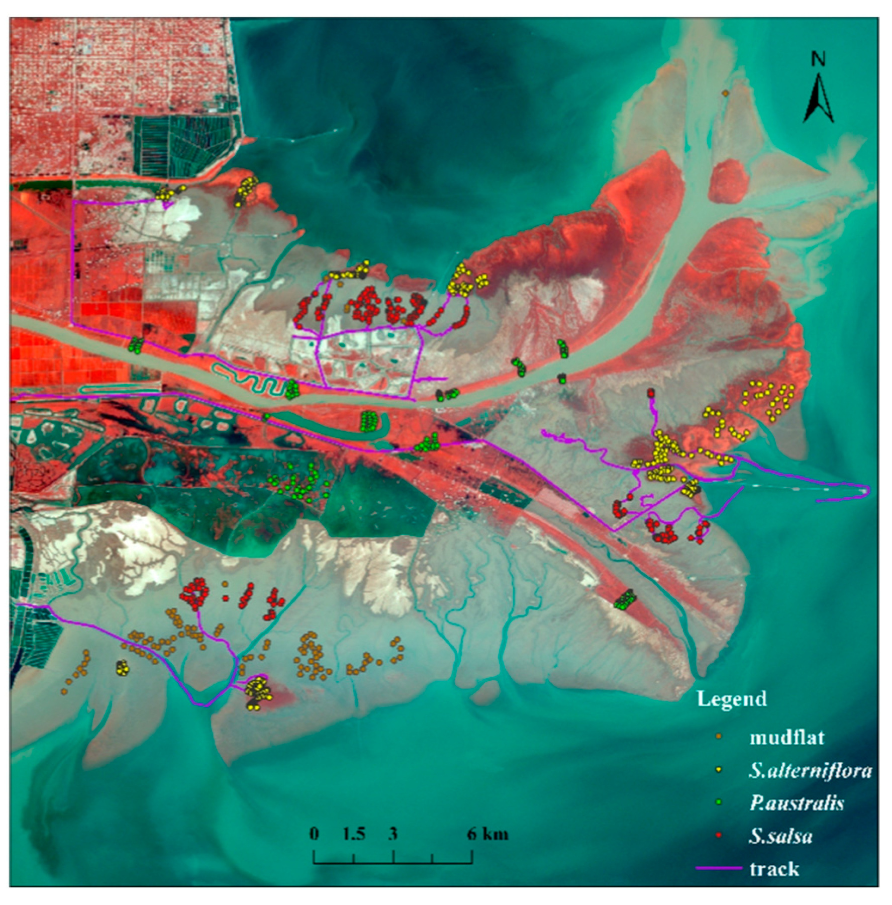
2.1. Study Area

The Yellow River Estuary Wetland (37°38′45″ N~37°55′15″ N, 119°01′30″ E~119°19′45″ E) is located in the estuary of the Yellow River in Dongying City, Shandong Province (Figure 1). Located at the land-sea interface, the Yellow River Delta experiences a warm temperate semi-humid continental monsoon climate. The topography of this area is generally gentle, sloping from southwest to northeast along the direction of the Yellow River. The natural vegetation of the study area is prominently represented by salt marsh meadows. Among the communities in the study area, Phragmites australis (P. australis,), Suaeda salsa (S. salsa), and Spartina alterniflora (S. alterniflora) account for about 60% of the total biomass and are typical of the dominant salt marsh vegetation.

2.2. Construction of the Annual Time Series Salt Marsh Vegetation Dataset

The vegetation classification in this study was performed using the random forest (RF) algorithm, an ensemble learning method that aggregates predictions from multiple decision trees through majority voting to determine the optimal classification outcome [15]. This algorithm demonstrates three distinctive advantages: (1) robustness to missing data and multicollinearity among predictor variables; (2) the inherent ability to handle high-dimensional feature spaces without requiring dimensionality reduction; and (3) enhanced classification accuracy without substantial computational overhead, making it currently one of the most effective machine learning approaches for vegetation mapping. The implementation procedure comprised three key phases: 1. development of a multidimensional temporal feature set incorporating spectral, temporal, and phenological characteristics across the study period; 2. creation of representative sample datasets through stratified random sampling of reference data; and 3. large-scale temporal classification of salt marsh vegetation using cloud-based computational infrastructure (Google Earth Engine, https://developers.google.com/earth-engine?hl=zh-cn, accessed on 20 February 2025), enabling the efficient processing of long-term satellite image series.

2.2.1. Development of the Multidimensional Feature Set

The Google Earth Engine (GEE) platform integrates data, model algorithms and computational resources in the cloud, providing great potential for processing and analyzing large-scale remote sensing data [34]. We obtained Landsat imagery (2000–2016) and Sentinel-2 data (2016–2021) covering the entire study area through the GEE platform. The obtained remote sensing data were 2A image products that were radiometrically and geometrically corrected. Images with cloud coverage ≤ 15% were filtered based on the embedded quality assessment metadata. Subsequently, cloud masking was applied to all filtered images to generate a complete dataset of cloud-free time series imagery. Both Landsat and Sentinel are equipped with multispectral sensors that capture reflectance data in multiple spectral bands (e.g., visible, red-edge, near-infrared). Building upon the dataset, various spectral indices were calculated based on specific combinations of bands throughout the vegetation growing season (April to September) to derive spectral dimension features (see Table 1 for detailed formulas). Spatial dimension features were generated through texture analysis using the gray-level co-occurrence matrix (GLCM) method.
To enhance classification accuracy while maintaining computational efficiency, feature selection was performed using the recursive feature elimination (RFE) method. The optimized feature subset (Table 1), comprising both spectral and spatial characteristics, was subsequently integrated as additional bands into the classification imagery.

2.2.2. Construction of the Sample Sets

In recent years, our research group has conducted numerous field expeditions to the study area. The field survey was primarily conducted along three routes (Appendix A Figure A1), with sampling points strategically positioned to encompass the major land features and typical salt marsh vegetation within the study area. Spectral data of salt marsh vegetation in various growth stages were collected using an ASD FieldSpec 3 back-suspended spectrometer (Lica United, Beijing, China), with a sampling spectrum range of 350–2500 nm and a front field angle of 25° for the optical fiber. Additionally, the GPS locations of the samples representing typical salt marsh vegetation were recorded. The initial sample points were manually verified using high-resolution Google Earth imagery and time-series data from GEE (Google Earth Engine), ensuring the accuracy and reliability of the classified sample points for the study area (Appendix A Table A1 displays the interpretation signs). The initial sample points were manually verified using high-resolution Google Earth imagery, ensuring the accuracy and reliability of the classified sample points for the study area. Given the extended duration of the study, a separate sample set was constructed for each year, incorporating time-series data from GEE as complementary information sources. Based on field conditions, 500–800 sampling points were selectively chosen each year, resulting in a comprehensive dataset of approximately 16,000 sampling sites spanning the period from 2000 to 2021. This systematic approach enabled the establishment of a temporally balanced sample set with uniform distribution across the 21-year study period.

2.2.3. Extraction of Long-Term Time-Series Salt Marsh Vegetation Data Based on GEE

The random forest (RF) classification algorithm was implemented using the ‘Classifier.smileRandomForest()’ program within the GEE platform to generate distribution maps of salt marsh vegetation. The sample set was divided into training and validation subsets through a randomized segmentation algorithm in the ratio of 7:3. Specifically, multi-source remote sensing data, including Landsat and Sentinel imagery, were sampled over 70% of the sample points to generate training datasets for RF classifier development, while the remaining 30% served as an independent validation set for rigorous performance evaluation and robustness assessment of the classification accuracy.

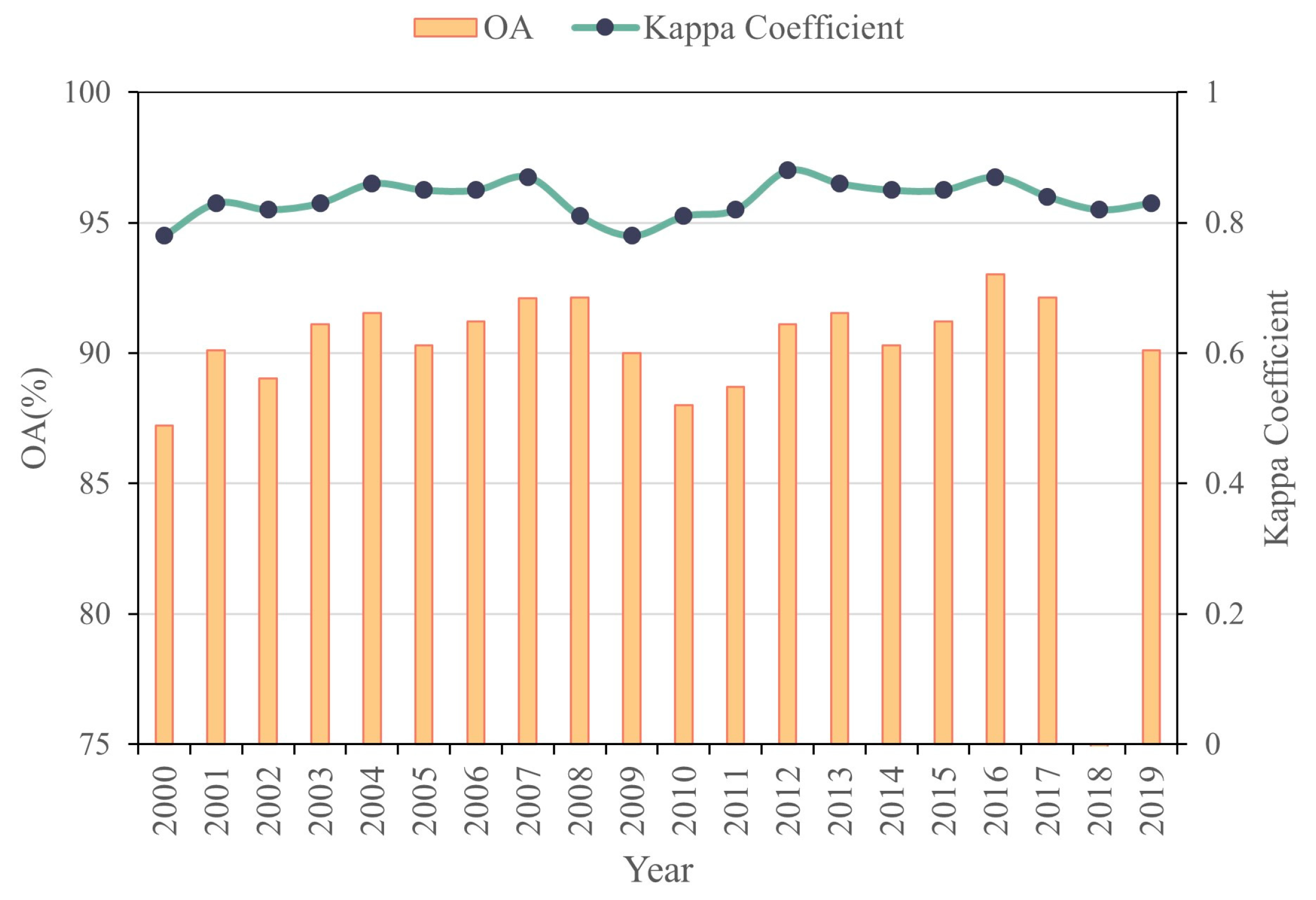
2.2.4. Accuracy Verification Method

In this study, the widely used overall accuracy (OA) and Kappa coefficient were used to evaluate the extraction accuracy of typical salt marsh vegetation [35]. The OA is the ratio of the number of correctly classified pixels to the total number of pixels, which indicates the accuracy of the overall pixel classification. The Kappa coefficient can be used to assess the quality of a classification and can overcome the sample and methodological dependence inherent in measuring classification accuracy using only the accuracy analysis metrics described above. The Kappa coefficient is calculated using the following formula:
K a p p a = p o p e 1 p e
p e = a 1 × b 1 + a 2 × b 2 + + a c × b c n × n
where p o represents the quotient obtained by dividing the number of samples correctly classified in each category by the total number of samples; in other words, it denotes the overall classification accuracy. a 1 , a 2 , ..., a c represents the number of accurately classified samples per category; b 1 , b 2 , ..., b c indicates the quantity of anticipated samples in each category; and n denotes the aggregate sample count.

2.3. Spatio-Temporal Succession Patterns of Salt Marsh Vegetation at the Landscape Scale

As a commonly used method of landscape pattern analysis, the landscape pattern index (LPI) can provide a high-level overview of the composition and spatial configuration of landscape patches [36]. Based on the monitoring results of salt marsh vegetation in the Yellow River Delta from 2000 to 2021, the LPI of salt marsh vegetation was calculated for each period using ArcGIS (10.7) and Fragstats (4.2.1) software. Nine indexes (Table 2), including the percentage of landscape (PLAND), patch density (PD), splitting Index (SPLIT), edge density (ED), landscape shape index (LSI), mean patch fractal dimension (PAFRAC), interspersion and juxtaposition index (IJI), patch cohesion index (COHESION), and aggregation index (AI) were used to describe the succession of S. alterniflora and S. salsa. The significance of the observed trend was subsequently analyzed using the Mann-Kendall trend test. The formula for determining the significance of the trend is as follows:
S = i = 1 n 1 j = j + 1 n s g n x j x i
S is the test statistic. When the length of the time series meets specific conditions (n ≥ 10), the statistic S can be approximately regarded as following a standard normal distribution. In this case, the corresponding test statistic Z can be used for trend testing. Under the framework of a two-tailed trend test, given a significance level α, the critical value Z 1 α / 2  is obtained by referring to the standard normal distribution table. Combined with the value of β, the significance of the time-series trend is classified as significant, non-significant, or no trend.

2.4. Spatio-Temporal Succession Patterns of Salt Marsh Vegetation at the Pixel Scale

We conducted pixel-scale monitoring of vegetation type variations, involving the examination of individual spatial units, subsequently transforming the evolving spatial unit data to facilitate the extraction of flow information [37]. The spatial variability of salt marsh vegetation was quantified through pixel-based change detection analysis, comparing consecutive annual vegetation distribution maps over a two-year observation period. Three distinct transition states were identified using the following computational scheme: (1) a value of +1 indicates the conversion from other vegetation types to S. salsa, representing vegetation gain; (2) a value of 0 corresponds to stable pixels showing no vegetation type change; and (3) a value of −1 signifies the transition from S. salsa to other vegetation types, indicating vegetation loss or degradation.
D T = G a i n i   ( M a p i M a p i 1 = 1 ) N O   c h a n g e   ( M a p i M a p i 1 = 0 ) L o s s i   ( M a p i M a p i 1 = 1 )
Furthermore, the spatial distribution frequency of S. salsa (p) was quantitatively assessed through pixel occurrence analysis, calculated as the ratio of S. salsa-identified pixels to the total number of valid pixels within the study area (N) using the following formula:
P = I = 2000 2021 M a p i N

2.5. Methods for Analyzing Coupled Interactions

2.5.1. Coupling Coefficients

The coupling coefficient (SCI), or elasticity coefficient [38,39], is often used to characterize the relationship between the growth rates of two indicators. In this study, the coupling coefficient was introduced to quantify the spatial coupling relationship between the distribution frequency of S. salsa and S. alterniflora and the distribution of tidal creeks, expressed as follows:
S C I = M i + N i 2 ( M i ) 2 + ( N i ) 2
N i represents the frequency of distribution of salt marsh vegetation (in this study, specifically referring to S. alterniflora and S. salsa) within the grid. M i is the number of tidal creeks in the grid. The value of SCI ranges from 0 to 1. The self-organizing process wherein increased salt marsh vegetation frequency reduces its separation distance from tidal creeks manifests as systematically higher SCI values in grids with equivalent channel numbers [40].
The coupling between the distribution frequency of salt marsh vegetation and the distribution pattern of tidal creeks reaches its peak when the absolute values of both M i and N i are equal, with one being positive and the other negative. When M i and N i are opposite numbers to each other, the coupling relationship between the distribution frequency of salt marsh vegetation and the distribution of tidal creeks is the weakest.

2.5.2. GeoDetector Model

GeoDetector is an open source statistical model for spatial data analysis (http://www.GeoDetector.cn/, accessed on 6 Apirl 2022) and is used to determine the similarity of the spatial distribution of two variables by considering spatially stratified heterogeneity [41]. GeoDetector consists of factor, interaction, risk, and ecological detectors. In this study, we chose the factor detector in the GeoDetector model to detect the spatial divergence of salt marsh vegetation, as well as to detect the ability of tidal creek morphological features to explain the spatial divergence of salt marsh vegetation. The factor detector model can be expressed as follows:
E X P = 1 h = 1 L N h Ϭ h 2 N Ϭ 2 = 1 S S W S S T
S S W = h = 1 L N h Ϭ h 2 , S S T = N Ϭ 2
The study area can be divided into L layers, denoted as h = 1, 2, 3, ..., L. Each layer, as well as the entire area is composed of several units, which are respectively recorded as N h and N. Ϭ h 2 and Ϭ 2 represent the variances of the Y values for layer h and the entire area, respectively. SSW and SST respectively represent the sum of the within-layer variances and the total variance of the entire area. Using this modeling framework, we conducted annual analyses of the coupling relationships between tidal creek morphological characteristics and salt marsh vegetation distribution patterns. This approach ultimately quantified both the explanatory power of creek morphology on vegetation spatial heterogeneity and its temporal dynamics.

3. Results

3.1. Spatial Distribution of Salt Marsh Vegetation

The salt marsh vegetation classification dataset (2000–2021) developed in this study demonstrated high accuracy, with overall classification accuracy ranging from 85% to 94% and Kappa coefficients between 0.82 and 0.87 (Figure 2). The classification error was maintained below 9%, meeting the accuracy requirements for the intended research applications.
According to the classification results, the vegetation in the study area is characterized by a regular gradient distribution. From the riverbank outward on both sides, a distinct zonation pattern was observed, with P. australis, S. salsa, and S. alterniflora distributed sequentially along the gradient. With the widest distribution area and overall stability, the spatial pattern of P. australis changed significantly with the fluctuation of the Yellow River terminal. Compared to that in 2002, there was a decrease in the area of P. australis by 2005. Later, with the implementation of the wetland restoration project, the wetland water area in the reserve expanded, and the area of P. australis gradually increased. The area of P. australis reached the highest value of 11,216 hm2 in 2017, representing an increase of 4527.27 hm2 compared to that in 1999. The area of P. australis decreased slightly after 2017 (Figure 3).
The area of S. salsa decreased rapidly from 10,214.03 hm2 to 6792 hm2 in the period of 2000–2015, with the most obvious decline occurring in the direction of the seaward extension of the current river channel. There was a temporary increase in the area covered by S. salsa after 2005, and it reached an area of 8707 hm2 in 2008. S. salsa continued to decline after 2010, with the sharpest drop occurring between 2010 and 2013, at which time S. alterniflora expanded rapidly. There was only 4945.14 hm2 of S. salsa in 2020, with an annual loss of about 75.86 hm2 on average.
Since 2008, a relatively small amount of S. alterniflora (about 7.5 hm2) has appeared in the coastal area in the north of the study area. It expanded rapidly along the coastal mudflats and newly sedimented mudflats at the mouth of the estuary, reaching an area of 1513.16 hm2 by 2013. It had spread to the halcyon mudflats along both sides of the Yellow River estuary by 2015.

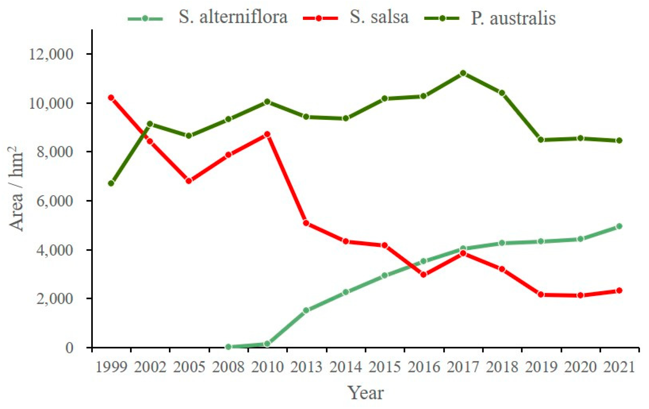
3.2. Evolution of Salt Marsh Vegetation at the Landscape Scale

The time series of landscape indexes for S. salsa and S. alterniflora exhibited distinct dynamics (Figure 4). Regarding the trend of the proportion of the landscape area occupied by both vegetation types (PLAND), S. salsa showed a significant declining trend, particularly after the invasion of S. alterniflora in 2008, while the invader’s coverage increased monotonically. The positive trend in S. salsa’s PD contrasted with S. alterniflora’s stable PD, suggesting the fragmentation of native vegetation. The cohesion index (COHESION) and aggregation index (AI) of both species displayed phased changes. S. alterniflora initially surged to an index value of 99.35 before stabilizing, indicating the rapid coalescence of invasion fronts. S. salsa maintained lower but stable COHESION after 2010, while its AI fluctuations reflected landscape-scale instability from competitive displacement.

3.3. Evolution of Salt Marsh Vegetation at the Pixel Scale

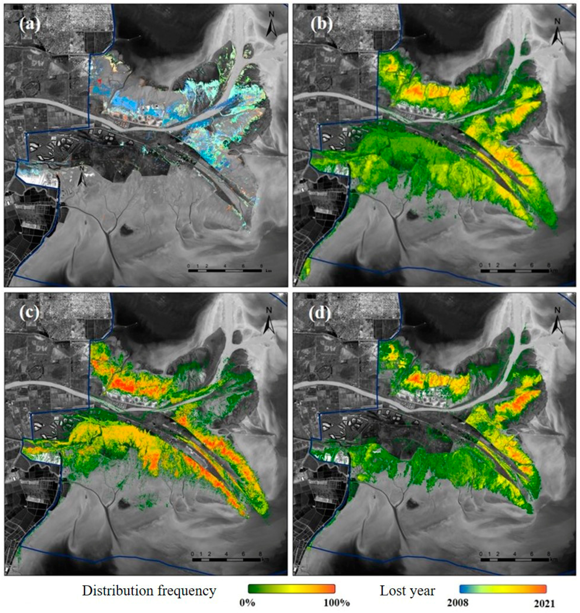
3.3.1. Variation in the State of Distribution of Native Vegetation

Analysis of the temporal patterns of S. salsa degradation (Figure A1 in the Appendix A) revealed pronounced vegetation loss during the initial period following the Yellow River channel diversion [42]. Spatial analysis identified two primary degradation hotspots: (1) the proximal zones surrounding newly formed channel mouths, and (2) the erosional banks of pre-existing tidal channels, where vegetation decline exhibited the greatest severity.
As for the distribution frequency, S. salsa colonized extensive areas of the intertidal zone of the Yellow River Delta since 2000, yet over 50% of these populations exhibited low and unstable distribution frequencies. While recent observations showed no recurrence of the extensive degradation events characteristic of the initial diversion period, the spatial pattern of degradation has shifted landward, indicating a progressive inland retreat of affected zones. Comparative analysis of pre- and post-invasion periods demonstrates that S. alterniflora invasion has significantly altered S. salsa distribution patterns: (1) the species’ range along the northern coast has contracted relative to pre-invasion conditions; (2) the core distribution areas (medium-high frequency zones) have undergone a northward displacement.

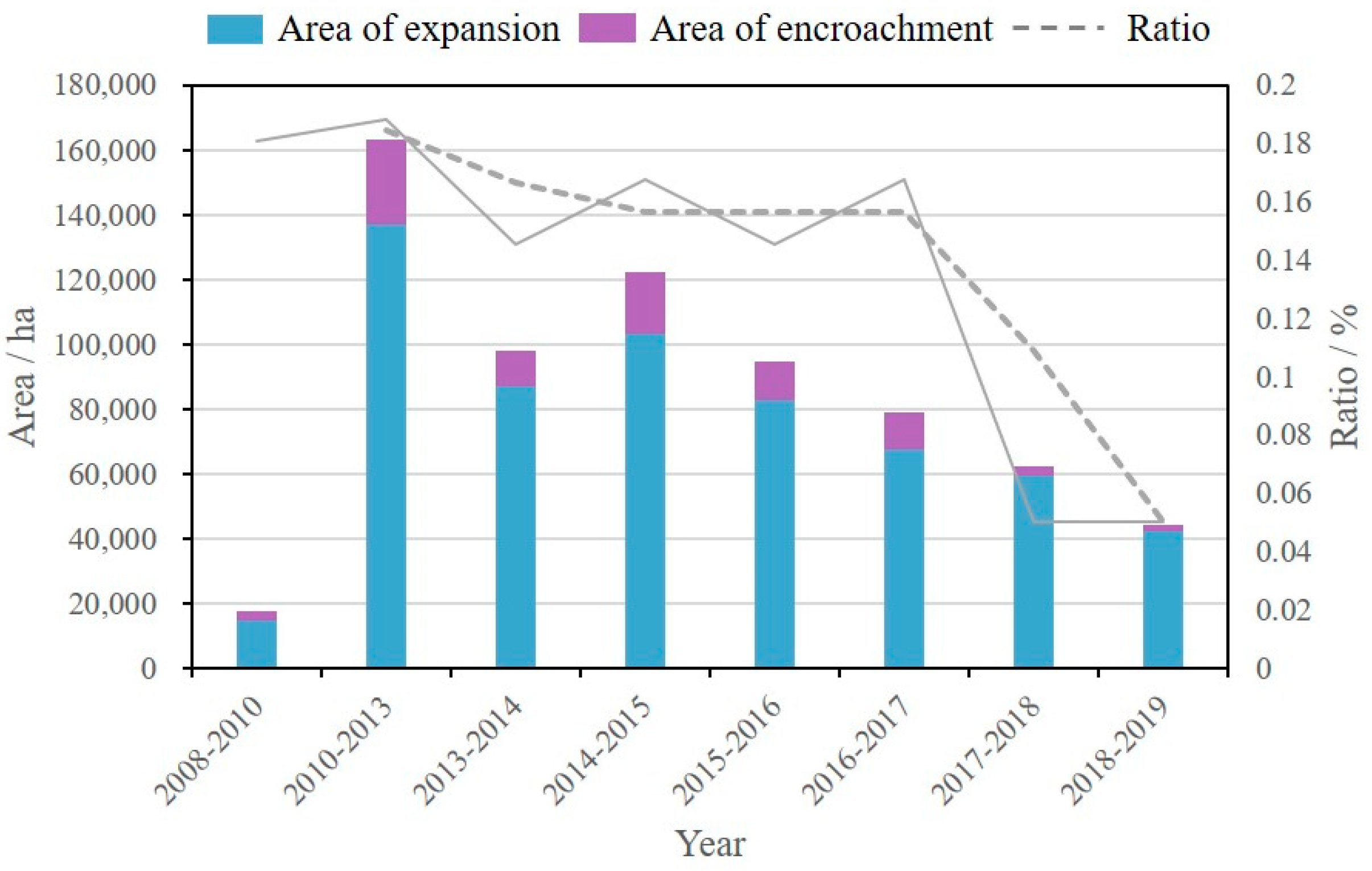
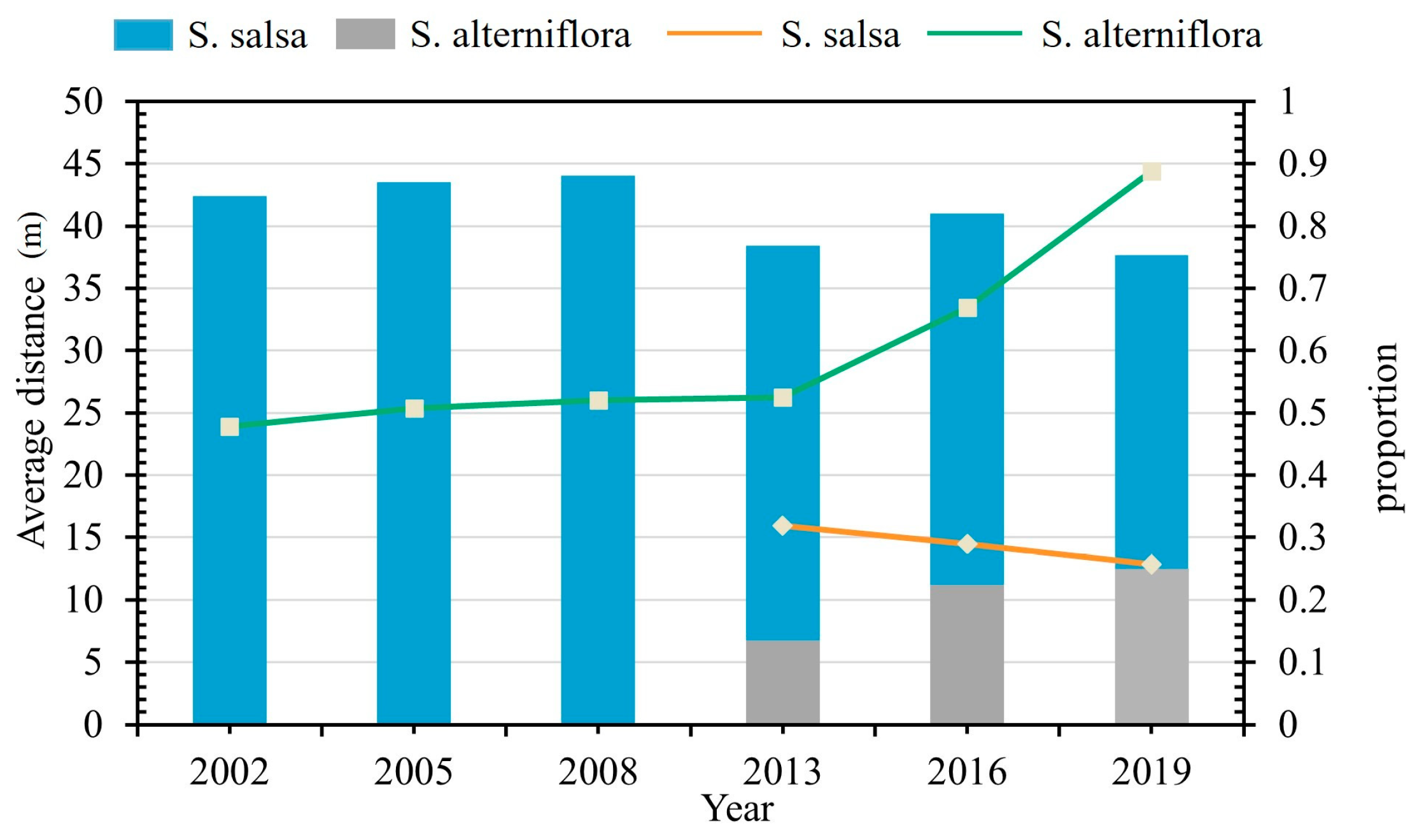
3.3.2. Occupation of Native Vegetation by S. alterniflora

The competitive encroachment S. alterniflora predominantly manifests along its landward expansion front, where the direct displacement of S. salsa populations is most pronounced. After settlement, S. alterniflora rapidly expands outward in a frontal shape to form continuous patches, and its maximum expansion area can reach 2583.09 hm2. However, the direct encroachment of S. alterniflora on S. salsa covers only about 13.5% of the expansion area and is declining, with a ratio of about 3.9% in 2021 (Figure 5). Although the direct encroachment of S. alterniflora on S. salsa as a proportion of S. alterniflora expansion continues to decline, the location of the interaction zone between S. alterniflora and S. salsa continues to move deeper onto land.

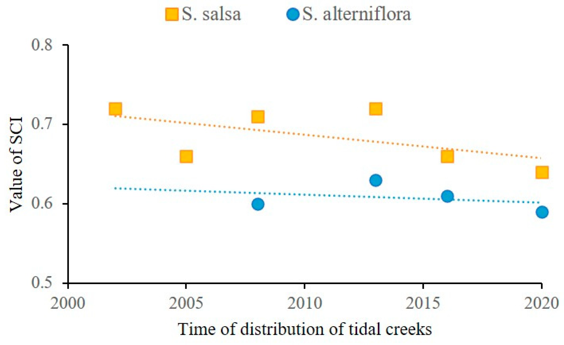
3.4. Relationship Between Salt Marsh Vegetation and Tidal Creeks

A systematic grid-based analysis was conducted using a 500 m × 500 m grid system across the study area. Through spatial linkage analysis, we quantified two key parameters: (1) the areal proportion of salt marsh vegetation within each grid unit, and (2) the mean distance between vegetation patches and tidal creeks. Figure 6 illustrates the spatio-temporal dynamics of tidal creek networks in relation to salt marsh vegetation communities (S. alterniflora and S. salsa), particularly before and after critical intervention periods, including water–sediment regulation tests (2002), wetland rehabilitation projects (2005), and vegetation restoration experiments (2013). In the graphical representation, the bar plots denote vegetation coverage proportions, while the line graphs indicate the corresponding mean distance measurements.
Before the invasion of S. alterniflora, the distributional proportion of S. salsa near the tidal creek was fairly stable and generally higher than 40 percent. The distance between S. salsa and the tidal creek system also remained relatively constant at around 25 m. With the expansion of the invasion of S. alterniflora, the area proportion of S. salsa near the tidal creek decreased significantly, and the area proportion of S. alterniflora increased rapidly. A more obvious pattern is indicated by the fact that the invasion of S. alterniflora occupied a position closer to the tidal creek, and the distance between S. salsa and the tidal creek expanded rapidly. Although the direct invasion of S. alterniflora on the ecological niche of S. salsa is insignificant, it has a certain impact on the development of tidal creeks, and the changes in the development of tidal creeks directly affect the spatial distribution of S. salsa.

3.4.1. Interaction Studies Based on Coupling Coefficients

Figure 7 shows the coupling relationship between the distribution of the two vegetation types and the distribution of tidal creeks. The linkage between the distribution frequency of S. salsa and the distribution of tidal creeks was generally stronger than that between the distribution frequency of S. alterniflora and the distribution of tidal creeks from 2000 to the present. These findings indicate that S. salsa, in contrast to S. alterniflora, has a closer connection to soil moisture and salinity levels, making its proliferation and spread more reliant on tidal creeks. There was a consistent correlation between the distribution frequency of S. alterniflora and the distribution of tidal creeks. Over time, the linkage between the distribution frequency of S. salsa and the distribution of tidal creeks decreased, with values closer to the linkage between the distribution frequency of S. alterniflora and tidal creeks.

3.4.2. Interaction Studies Based on the GeoDetector Model

The results of measuring how the morphological characteristics of tidal creeks influence the structural heterogeneity of salt marsh vegetation using the GeoDetector model are shown in Figure 8. Exp values produced by length of tidal creeks were the highest for salt marsh vegetation structure, while those for the curvature of tidal creeks were slightly lower. From 2004 to 2020, there was a slight increase in the Exp values for the length and curvature of tidal creeks in relation to the structural heterogeneity of salt marsh vegetation, rising from 0.54 and 0.42 to 0.73 and 0.61, respectively. Additionally, the impact of tidal creek length and curvature on the structural heterogeneity of salt marsh vegetation exhibited a slight upward trend over time (Figure 9). The Exp associated with the tidal creek class in relation to the structure of salt marsh vegetation exhibited the smallest magnitude and remained consistently stable over time, approximately converging to a value of 0.08. This indicates that, compared to the first two factors, the tidal creek class contributes significantly less to the explanation of structural differentiation within salt marsh vegetation.

4. Discussion

4.1. Multiscale Structural Dynamics of Salt Marsh Vegetation

Based on the analysis of the results of long-term time-series monitoring of salt marsh vegetation in the intertidal zone of the Yellow River Delta, it was found that the vegetation in the study area exhibits obvious gradient distribution characteristics. Our findings on the changes in the landscape patterns of salt marsh vegetation demonstrate that the landscape pattern evolution of salt marsh vegetation represents a complex interplay of biotic and abiotic factors, reflecting both spatial distribution characteristics and temporal dynamics that fundamentally influence associated ecological processes [43]. The invasion of S. alterniflora has significantly altered the intertidal environment, particularly through modifications to soil hydro-saline conditions. Our results indicate that the differential adaptation strategies and feedback mechanisms between S. salsa and S. alterniflora in response to varying hydro-saline environments are crucial drivers of habitat encroachment, particularly in ecotonal areas adjacent to S. alterniflora colonies. The observed inland expansion of the interspersed zone between these two species presents increasing challenges for S. salsa’s growth and survival, as evidenced by the declining landscape metrics and distribution frequency patterns. The spatial-temporal analysis reveals that S. salsa degradation has progressively shifted inland, with the most severe impacts concentrated along newly formed channels and eroded sections of pre-existing channels. This phenomenon suggests that hydrological modifications, combined with competitive pressure from S. alterniflora, have created a complex stress regime for native vegetation. The northward shift of medium- and high-distribution frequency areas of S. salsa, despite overall range contraction, indicates potential adaptation responses to changing environmental conditions.
However, this study has certain limitations that warrant consideration in future research. First, our analysis did not fully account for the potential impacts of climate change factors, particularly sea-level rise and associated salinity changes. Second, the potential synergistic effects between biological invasions and climate change factors remain poorly understood and require further investigation. Future studies should incorporate predictive modeling approaches to assess long-term vegetation dynamics under combined pressures of biological invasions and climate change scenarios.

4.2. The Interaction of Salt Marsh Vegetation Coupled with Tidal Creeks

The spatio-temporal dynamics of salt marsh vegetation in relation to tidal creek systems reveal complex ecological processes shaped by both abiotic factors and interspecies competition. Previous studies have demonstrated that tidal creek systems exhibit pronounced elevation gradients and dynamic hydrological variations along their banks. This spatial heterogeneity creates distinctive micro-environmental patterns that exert deterministic control over the colonization, development, and spatial distribution of salt marsh vegetation. The proximity to tidal creeks proves particularly favorable for S. salsa colonization, as evidenced by higher seed arrival rates, germination success, and seedling survival in these areas, consistent with previous studies on hydrochorous dispersal mechanisms in tidal environments [44,45]. The invasion of S. alterniflora has substantially altered these established patterns, with the invasive species preferentially colonizing areas closer to tidal creeks. This spatial reorganization has led to the displacement of S. salsa populations, increasing their average distance from tidal creeks from a stable 25 m to significantly greater values. While the direct niche overlap between the two species appears limited, our results suggest that S. alterniflora’s impact on tidal creek development has created indirect competitive pressures on S. salsa. The formation of dense S. alterniflora communities along narrow tidal channels has effectively restricted channel extension into S. salsa habitats, contributing to the observed degradation of S. salsa in intertidal transition zones. The differential coupling relationships between vegetation distribution and tidal creek systems provide important insights into species-specific ecological adaptations. The stronger and more variable linkage between S. salsa distribution and tidal creeks (SCI = 0.64–0.73) compared to that for S. alterniflora (SCI = 0.59–0.63) suggests that native species are more sensitive to hydro-saline conditions mediated by tidal creek dynamics. This finding aligns with the ecological principle that native species typically exhibit more specialized adaptations to local environmental conditions than invasive species [46]. The temporal decrease in the SCI value of S. salsa indicates a reduction in the stability of the interdependent relationship between native vegetation and tidal creek systems, potentially reflecting an ecosystem response to changing environmental conditions under vegetation invasion.
However, this study has certain limitations that should be addressed in future research. First, while we have focused on tidal creek–vegetation interactions, other environmental variables such as sediment nutrient dynamics, microtopographic variations, and interspecific belowground competition were not fully considered. Second, the potential impacts of climate change factors, particularly sea-level rise and changing precipitation patterns, were not incorporated into our analysis. These factors could alter tidal creek morphology and hydroperiods, potentially amplifying or mitigating the observed vegetation dynamics. While the GeoDetector model effectively identified key spatial drivers of vegetation distribution, its discrete time-slice approach may obscure finer-scale ecological processes that operate beyond our sampling intervals, warranting the careful interpretation of temporal dynamics. Future studies can integrate complementary approaches to address these gaps: (1) dynamic Bayesian network modeling to capture time-dependent relationships; (2) higher-frequency remote sensing observations (e.g., monthly composites); and (3) process-based models that explicitly simulate temporal vegetation responses.

5. Conclusions

This study employed the GEE cloud platform to reconstruct annual salt marsh vegetation distributions from 2000 to 2019, enabling comprehensive landscape-scale analysis of spatio-temporal patterns. Our findings reveal three key insights: First, the study area exhibits distinct gradient distribution patterns of salt marsh vegetation. Pixel-based succession analysis of S. salsa and S. alterniflora demonstrates that S. salsa degradation is primarily driven by hydrological alterations from anthropogenic activities (particularly Yellow River diversion), with S. alterniflora invasion playing a secondary role. Second, vegetation–tidal creek coupling analysis indicates that S. alterniflora invasion significantly modifies intertidal geomorphology, thereby influencing tidal creek development. These geomorphological changes create feedback mechanisms that further affect vegetation dynamics. Third, we identify critical vulnerability points in S. salsa life history: all life stages (seed production, dispersal, and retention) exhibit heightened sensitivity to hydrological conditions. Particularly noteworthy is the inhibitory effect of tidal creek blockage and associated edaphic changes resulting from S. alterniflora expansion—a crucial consideration for future restoration efforts.

Author Contributions

Conceptualization, J.H. and Z.G.; methodology, J.H.; software, J.H.; validation, J.H., J.Y. and Z.B.; formal analysis, D.Z.; investigation, J.H.; resources, Z.G.; data curation, J.Y.; writing—original draft preparation, J.H.; writing—review and editing, J.Y. and Z.B.; visualization, J.H. and D.Z.; supervision, J.Y.; project administration, Z.B.; funding acquisition, J.H. All authors have read and agreed to the published version of the manuscript.

Funding

This research was funded by the Science and Innovation Fund of the Center for Geophysical Survey, grant number DKC20230004.

Data Availability Statement

The raw data supporting the conclusions of this article will be made available by the authors on request.

Conflicts of Interest

The authors declare no conflicts of interest. The funders had no role in the design of the study; in the collection, analyses, or interpretation of data; in the writing of the manuscript; or in the decision to publish the results.

Abbreviations

The following abbreviations are used in this manuscript:
S. salsaSuaeda salsa
S. alternifloraSpartina alterniflora
P. australisPhragmites australis

Appendix A

Figure A1. Sampling locations and survey transects (adapted from [47]).
Jmse 13 00946 g0a1
Table A1. Signs for the remote sensing interpretation of salt marsh vegetation.
Interpreting SignsDescriptionImage Features (False Color)
Suaeda salsaScattered across coastal tidal flats; exhibits pinkish-red hues in false-color composites; typically shows low-density growth patterns
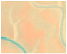
Jmse 13 00946 i001
Phragmites australisForms continuous patches along riverbanks and waterfronts; distinct red coloration in false-color imagery; demonstrates linear distribution following hydrological features
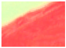
Jmse 13 00946 i002
Spartina alternifloraConcentrated in intertidal zones; deep red tones in false-color representations; characterized by high-density canopy coverage
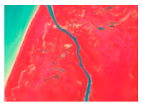
Jmse 13 00946 i003

References

  1. Gong, J.; Li, B.; Liu, C.; Li, P.; Hu, J.; Yang, G. Impact of salinity gradients on nitric oxide emissions and functional microbes in estuarine wetland sediments. Water Res. 2025, 273, 123046. [Google Scholar] [CrossRef] [PubMed]
  2. Hu, W.; Chen, M.; Lan, X.; Li, G.; Wang, B.; Sun, D.Y.; Lin, X.B. Shifts of ammonia-oxidation process along salinity gradient in an estuarine wetland. Ecol. Indic. 2022, 145, 109655. [Google Scholar] [CrossRef]
  3. Wei, H.; Gao, D.; Liu, Y.; Lin, X. Sediment nitrate reduction processes in response to environmental gradients along an urban river-estuary-sea continuum. Sci. Total Environ. 2020, 718, 137185. [Google Scholar] [CrossRef] [PubMed]
  4. Gong, J.; Li, B.; Hu, J.; Li, P.; Liu, Q.; Yang, G.; Liu, C. Driving force of tidal pulses on denitrifiers-dominated nitrogen oxide emissions from intertidal wetland sediments. Water Res. 2023, 247, 120770. [Google Scholar] [CrossRef]
  5. Douglas, E.J.; Lam-Gordillo, O.; Hailes, S.; Lohrer, A.; Cummings, V.J. Characterising intertidal sediment temperature gradients in estuarine systems. Estuar. Coast. Shelf Sci. 2024, 309, 108968. [Google Scholar] [CrossRef]
  6. Loi, L.T.; Phong, N.T.; Nguyen, L.T. Intertidal bare mudflat and wave attenuation: A case study in the Vietnamese Mekong Delta. Ecol. Eng. 2024, 206, 107320. [Google Scholar] [CrossRef]
  7. Marani, M.; Da Lio, C.; D’Alpaos, A. Vegetation engineers marsh morphology through multiple competing stable states. Proc. Natl. Acad. Sci. USA 2013, 110, 3259–3263. [Google Scholar] [CrossRef]
  8. Dzimballa, S.; Willemsen, P.W.J.M.; Kitsikoudis, V.; Borsje, B.W.; Augustijn, D.C.M. Numerical modelling of biogeomorphological processes in salt marsh development: Do short-term vegetation dynamics influence long-term development. Geomorphology 2025, 471, 109534. [Google Scholar] [CrossRef]
  9. Xie, T.; Cui, B.; Bai, J.; Li, S.; Zhang, S. Rethinking the role of edaphic condition in halophyte vegetation degradation on salt marshes due to coastal defense structure. Phys. Chem. Earth Parts A/B/C 2018, 103, 81–90. [Google Scholar] [CrossRef]
  10. Murray, N.J.; Phinn, S.R.; Dewitt, M.; Ferrari, R.; Johnston, R.; Lyons, M.B.; Clinton, N.; Thau, D.; Fuller, R. The global distribution and trajectory of tidal flats. Nature 2019, 565, 222–225. [Google Scholar] [CrossRef]
  11. Song, S.; Wu, Z.; Wang, Y.; Cao, Z.; He, Z.; Su, Y. Mapping the Rapid Decline of the Intertidal Wetlands of China Over the Past Half Century Based on Remote Sensing. Front. Earth Sci. 2020, 8, 16. [Google Scholar] [CrossRef]
  12. Ouyang, Z.T.; Zhang, M.Q.; Xie, X.; Shen, Q.; Guo, H.; Zhao, B. A comparison of pixel-based and object-oriented approaches to VHR imagery for mapping saltmarsh plants. Ecol. Inform. 2011, 6, 136–146. [Google Scholar] [CrossRef]
  13. Kumar, L.; Sinha, P. Mapping salt-marsh land-cover vegetation using high-spatial and hyperspectral satellite data to assist wetland inventory. Mapp. Sci. Remote Sens. 2014, 51, 483–497. [Google Scholar] [CrossRef]
  14. Zeng, J.; Sun, Y.; Cao, P.; Wang, H. A phenology-based vegetation index classification (PVC) algorithm for coastal salt marshes using Landsat 8 images. Int. J. Appl. Earth Obs. Geoinf. 2022, 110, 102776. [Google Scholar] [CrossRef]
  15. Dong, D.; Wang, C.; Yan, J.; He, Q.; Zeng, J.; Wei, Z. Combing Sentinel-1 and Sentinel-2 image time series for invasive Spartina alterniflora mapping on Google Earth Engine: A case study in Zhangjiang Estuary. J. Appl. Remote Sens. 2020, 14, 044504. [Google Scholar]
  16. Yi, W.; Wang, N.; Yu, H.; Jiang, Y.; Zhang, D.; Li, X.; Lv, L.; Xie, Z. An enhanced monitoring method for spatio-temporal dynamics of salt marsh vegetation using google earth engine. Estuar. Coast. Shelf Sci. 2024, 298, 108658. [Google Scholar] [CrossRef]
  17. Wang, D.; Bai, J.; Gu, C.; Gao, W.; Zhang, C.; Gong, Z.; Cui, B. Scale-dependent biogeomorphic feedbacks control the tidal marsh evolution under Spartina alterniflora invasion. Sci. Total Environ. 2021, 776, 146495. [Google Scholar] [CrossRef]
  18. Wan, D.; Yu, P.; Kong, L.; Zhang, J.; Chen, Y.H.; Zhao, D.; Liu, J. Effects of inland salt marsh wetland degradation on plant community characteristics and soil properties. Ecol. Indic. 2024, 159, 111582. [Google Scholar] [CrossRef]
  19. Song, J.; Liang, Z.; Li, X.; Wang, X.; Chu, X.J.; Zhao, M.L.; Zhang, X.; Li, P.; Song, W.; Huang, W.; et al. Precipitation changes alter plant dominant species and functional groups by changing soil salinity in a coastal salt marsh. J. Environ. Manag. 2024, 368, 122235. [Google Scholar] [CrossRef]
  20. Lefor, M.W.; Kennard, W.C.; Civco, D.L. Relationships of salt-marsh plant distributions to tidal levels in Connecticut, USA. Environ. Manag. 1987, 11, 61–68. [Google Scholar] [CrossRef]
  21. Hickey, D.; Bruce, E. Examining Tidal Inundation and Salt Marsh Vegetation Distribution Patterns using Spatial Analysis (Botany Bay, Australia). J. Coast. Res. 2010, 26, 94–102. [Google Scholar] [CrossRef]
  22. Mariotti, G.; Fagherazzi, S. A numerical model for the coupled long-term evolution of salt marshes and tidal flats. J. Geophys. Res. Earth Surf. 2010, 115, F01004. [Google Scholar] [CrossRef]
  23. Best, Ü.S.N.; Van der Wegen, M.; Dijkstra, J.; Willemsen, P.; Borsje, B.W.; Roelvink, D.J.A. Do salt marshes survive sea level rise? Modelling wave action, morphodynamics and vegetation dynamics. Environ. Model. Softw. 2018, 109, 152–166. [Google Scholar] [CrossRef]
  24. Mariotti, G. Beyond marsh drowning: The many faces of marsh loss (and gain). Adv. Water Resour. 2020, 144 Pt B, 103710. [Google Scholar] [CrossRef]
  25. Hughes, Z.J. Tidal Channels on Tidal Flats and Marshes. In Principles of Tidal Sedimentology; Springer: Berlin/Heidelberg, Germany, 2012. [Google Scholar]
  26. Sullivan, J.C.; Torres, R.; Garrett, A.; Blanton, J.; Alexander, C.; Robinson, M.; Moore, T.; Amft, J.; Hayes, D. Complexity in salt marsh circulation for a semienclosed basin. J. Geophys. Res. Earth Surf. 2014, 120, 1973–1989. [Google Scholar] [CrossRef]
  27. van de Vijsel, R.C.; van Belzen, J.; Boum, T.J.; van der Wal, D.; Borsje, B.W.; Temmerman, S.; Cornacchia, L.; Gourgue, O.; van de Koppel , J. Vegetation controls on channel network complexity in coastal wetlands. Nat. Commun. 2023, 14, 7158. [Google Scholar]
  28. Mallin, M.A.; Lewitus, A.J. The importance of tidal creek ecosystems. J. Exp. Mar. Biol. Ecol. 2004, 298, 145–149. [Google Scholar] [CrossRef]
  29. Schwarz, C.; Gourgue, O.; van Belzen, J.; Zhu, Z.; Bouma, T.J.; van de Koppel, J.; Ruessink, G.; Claude, N.; Temmerman, S. Self-organization of a biogeomorphic landscape controlled by plant life-history traits. Nat. Geoence 2018, 11, 672–677. [Google Scholar]
  30. van Iersel, W.; Straatsma, M.; Addink, E.; Middelkoop, H. Monitoring height and greenness of non-woody floodplain vegetation with UAV time series. ISPRS J. Photogramm. Remote Sens. 2018, 141, 112–123. [Google Scholar]
  31. Tan, L.; Ge, Z.; Fei, B.; Xie, L.; Li, Y.; Li, S.; Li, X.; Ysebaert, T. The roles of vegetation, tide and sediment in the variability of carbon in the salt marsh dominated tidal creeks. Estuar. Coast. Shelf Sci. 2020, 239, 106752. [Google Scholar] [CrossRef]
  32. Cui, L.; Ke, Y.; Min, Y.; Han, Y.; Zhang, M.; Zhou, D.M. Effects of tidal creeks on Spartina Alterniflora expansion: A perspective from multi-scale remote sensing. Ecol. Indic. 2024, 160, 111842. [Google Scholar] [CrossRef]
  33. Gao, Y.; Yi, Y.; Chen, K.; Xie, H. Simulation of suitable habitats for typical vegetation in the Yellow River Estuary based on complex hydrodynamic processes. Ecol. Indic. 2023, 154, 110623. [Google Scholar] [CrossRef]
  34. Dezfooli, F.P.; Zoej, M.J.V.; Mansourian, A.; Youssefi, F.; Pirasteh, S. GEE-Based Environmental Monitoring and Phenology Correlation Investigation Using Support Vector Regression. Remote Sens. Appl. Soc. Environ. 2024, 37, 101445. [Google Scholar] [CrossRef]
  35. Deng, X.; Liu, Q.; Deng, Y.; Mahadevan, S. An improved method to construct basic probability assignment based on the confusion matrix for classification problem. Inf. Sci. 2016, 340, 250–261. [Google Scholar] [CrossRef]
  36. Xue, S.; Ma, B.; Wang, C.; Li, Z. Identifying key landscape pattern indices influencing the NPP: A case study of the upper and middle reaches of the Yellow River. Ecol. Model. 2023, 484, 110457. [Google Scholar] [CrossRef]
  37. Lan, S.; Zhang, Y.; Gao, T.; Tong, F.; Tian, Z.; Zhang, H.; Li, M.; Mustafa, N.S. UAV remote sensing monitoring of winter wheat tiller number based on vegetation pixel extraction and mixed-features selection. Int. J. Appl. Earth Obs. Geoinf. 2024, 131, 103940. [Google Scholar] [CrossRef]
  38. Wang, X.; Yang, J. A privacy image encryption algorithm based on piecewise coupled map lattice with multi dynamic coupling coefficient. Inf. Sci. 2021, 569, 217–240. [Google Scholar] [CrossRef]
  39. Aschonitis, V.G.; Gaglio, M.; Castaldelli, G.; Fano, E.A. Criticism on elasticity-sensitivity coefficient for assessing the robustness and sensitivity of ecosystem services values. Ecosyst. Serv. 2016, 20, 66–68. [Google Scholar] [CrossRef]
  40. Hou, W.; Liang, S.; Sun, Z.; Ma, Q.; Hu, X.; Zhang, R. Depositional dynamics and vegetation succession in self-organizing processes of deltaic marshes. Sci. Total Environ. 2024, 912, 169402. [Google Scholar] [CrossRef]
  41. Zhu, Y.; Ling, G.H.T. Driving forces and prediction of urban open spaces morphology: The case of Shanghai, China using geodetector and CA-Markov model. Ecol. Inform. 2024, 82, 102763. [Google Scholar] [CrossRef]
  42. Kong, D.; Miao, C.; Zheng, H.; Gong, J. Dynamic evolution characteristics of the Yellow River Delta in response to estuary diversion and a water-sediment regulation scheme. J. Hydrol. 2023, 627, 130447. [Google Scholar] [CrossRef]
  43. Wang, H.; Zhou, Y.; Wu, J.; Wang, C.X.; Zhang, R.; Xiong, X.; Xu, C. Human activities dominate a staged degradation pattern of coastal tidal wetlands in Jiangsu province, China. Ecol. Indic. 2023, 154, 110579. [Google Scholar] [CrossRef]
  44. Cui, B.; He, Q.; Zhao, X. Ecological thresholds of Suaeda salsa to the environmental gradients of water table depth and soil salinity. Acta Ecol. Sin. 2008, 28, 1408–1418. [Google Scholar] [CrossRef]
  45. Ma, X.; Qiu, D.; Wang, F.; Jiang, X.; Sui, H.C.; Liu, Z.; Yu, S.; Ning, Z.; Gao, F.; Bai, J.H.; et al. Tolerance between non-resource stress and an invader determines competition intensity and importance in an invaded estuary. Sci. Total Environ. 2020, 724, 138225. [Google Scholar] [CrossRef] [PubMed]
  46. Ning, Z.; Li, D.; Chen, C.; Xie, C.J.; Chen, G.; Xie, T.; Wang, Q.; Bai, J.H.; Cui, B.S. The importance of structural and functional characteristics of tidal channels to smooth cordgrass invasion in the Yellow River Delta, China: Implications for coastal wetland management. J. Environ. Manag. 2023, 342, 118297. [Google Scholar] [CrossRef]
  47. Zhang, C.; Gong, Z.; Qiu, H.; Zhang, Y.; Zhou, D. Mapping typical salt-marsh species in the yellow river delta wetland supported by temporal-spatial-spectral multidimensional features. Sci. Total Environ. 2021, 783, 147061. [Google Scholar] [CrossRef]
Figure 1. Study area.
Jmse 13 00946 g001
Figure 2. Distribution of accuracy.
Jmse 13 00946 g002
Figure 3. Changes in the area of salt marsh vegetation.
Jmse 13 00946 g003
Figure 4. Landscape pattern of S. salsa and S. alterniflora.
Jmse 13 00946 g004
Figure 5. Distribution state of S. salsa. (a) Degradation distribution map of S. salsa; (b) distribution frequency of S. salsa in 2000–2021; (c,d) distribution frequency of S. salsa before and after the invasion of S. alterniflora.
Jmse 13 00946 g005
Figure 6. Direct invasion of native vegetation by S. alterniflora (the solid line is the trend in the study area).
Jmse 13 00946 g006
Figure 7. Relationship between salt marsh vegetation and tidal creeks.
Jmse 13 00946 g007
Figure 8. SCI between the distribution frequency of salt marsh vegetation and tidal creeks (lines represent the trend lines of the SCI values.).
Jmse 13 00946 g008
Figure 9. Explanatory power of tidal creek morphological characteristics on the structural differentiation of salt marsh vegetation.
Jmse 13 00946 g009
Table 1. Multidimensional feature set.
FeatureSource ImagesAbbreviationDescriptionTime Scale
Spectral featuresSentinel-2, LandsatBSpectral reflectanceLandsat: growing seasons in 2000–2015
NDWI(G − NIR)/(G + NIR)
NDVI(NIR − R)/(NIR + R)
RDVI N D V I D V I Sentinel-2:
growing seasons in 2016–2021
DVINIR − R
MASVI 2 N I R + 1 ( 2 N I R + 1 ) 2 8 ( N I R R )
RVINIR/R
Sentinel-2NDVIre1(B8 − B5)/(B8 + B5)
NDVIre2(B8 − B6)/(B8 + B6)
NDVIre3(B8 − B7)/(B8 + B7)
Spatial featuresSentinel-2, LandsatASMangular second-order momentGrowing seasons in 2000–2021
CorCorrelation
ConContrast
Ententropy
Varvariance
Table 2. Landscape index list.
LPIFormulaDescription
Proportion of landscape area occupied by patches P L A N D = i = 1 n a i j A 100 Area characterizing patch type as a percentage of total landscape area
Patch density P D = N i A i Edge length between a landscape element patch and its adjacent heterogeneous patches
Fragmentation index S P L I T = A 2 1 M a i 2 Changes in the shape of landscape types
Edge density E D = 1 A j = 1 M P i j Complexity of patch shapes and patch edges in the landscape
Patch shape index L S I = 0.25 E A Extent to which topographic and hydrologic conditions affect this type of patch
Subdimensional index P A F R A C = 2 ln P 4 ln A Aggregated or dispersed state of patches in the landscape
Scattering and juxtaposition index I J I = i = 1 m k = i + 1 m e i k E ln e i k E ln 0.5 m m 1 × 100 Connectivity within landscape type patches
Cohesion index C O H E S I O N = 1 j = 1 m p i j j = 1 m p i j a i j 1 1 A 1 × 100 Degree of dispersion and aggregation within the same landscape type
Aggregation index A I = g i j m a x g i j × 100 Degree of landscape fragmentation and spatial heterogeneity
Disclaimer/Publisher’s Note: The statements, opinions and data contained in all publications are solely those of the individual author(s) and contributor(s) and not of MDPI and/or the editor(s). MDPI and/or the editor(s) disclaim responsibility for any injury to people or property resulting from any ideas, methods, instructions or products referred to in the content.

