Noise Characteristics and Shallow Subsurface Structure Detection in Coastal Zones: A Case Study from Dong’ao Island, Zhuhai

Abstract

Shallow subsurface structure detection in coastal zones serves as a critical foundation for resource development and engineering construction. However, conventional geophysical methods exhibit significant limitations in land–sea transition zones, where pronounced “boundary effects” create substantial “exploration gaps” due to difficulties in merging terrestrial and marine datasets. To achieve truly seamless subsurface imaging across the coastal boundary, this study develops and implements an integrated cross-boundary survey approach utilizing nodal seismometers and seismic ambient noise. At Dong’ao Island, Zhuhai, we deployed a comprehensive seismic profile spanning hillside, sandbeach, and seafloor environments to evaluate the method’s applicability in complex coastal settings systematically. Results demonstrate substantially stronger ambient noise energy in submarine environments compared to terrestrial settings. All stations recorded abundant and stable high-frequency (>1 Hz) noise signals, which are adequate for shallow subsurface imaging. Rayleigh wave dispersion curves extracted via the advanced Frequency-Bessel transform method enabled inversion of a continuous 2D shear-wave velocity profile along the survey line. Bedrock interface depths determined using the Horizontal-to-Vertical Spectral Ratio (HVSR) method showed remarkable consistency with the bedrock morphology revealed by the shear-wave velocity structure, validating the reliability of our approach in coastal environments. This research successfully demonstrates the feasibility of seismic ambient noise imaging as a bridging technique for land–sea exploration, providing an efficient, environmentally friendly, and continuous technical solution to overcome coastal zone exploration challenges.

1. Introduction

Coastal zones, characterized by intense land–sea interactions and concentrated human activities, represent critical frontiers where accurate subsurface characterization is fundamental to both geoscientific research and engineering development [1]. However, detection in these areas is significantly hampered by inherent limitations of conventional geophysical methods, creating pronounced “exploration gaps” at the terrestrial-marine transition. Specifically, marine seismic techniques (e.g., single-channel seismics, sub-bottom profiling) suffer from reduced effectiveness in nearshore hard-seafloor environments due to frequency constraints and water depth limitations. Conversely, terrestrial methods such as electrical resistivity are susceptible to environmental interference, compromising their accuracy, while drilling provides only sparse point data. A more fundamental challenge lies in the inherent discrepancies in resolution and processing standards between marine and terrestrial datasets, which hinder their effective integration [2,3]. Consequently, developing an effective geophysical approach capable of seamlessly bridging the land–sea boundary and providing continuous subsurface imaging is urgently needed to obtain a unified geological model of the coastal zone [4].

Seismic ambient noise imaging is an advanced technique that utilizes continuous background signals generated by natural sources (ocean waves, wind) and anthropogenic activities (traffic) to reconstruct subsurface structures. This method offers distinct advantages, including environmental friendliness (requiring no active sources and causing no surface damage), operational flexibility, high efficiency, and cost-effectiveness [5,6]. Over recent decades, the technique has undergone rapid development in land applications, expanding its scope to numerous domains: high-resolution imaging of Earth’s interior at global and regional scales [7,8,9], detection of subsurface geological structures and mining goafs [10,11,12], detection of near-surface structures on celestial bodies [13,14,15], urban engineering geology and marine site characterization [16,17,18], as well as geohazard monitoring and early warning systems for landslides, earthquakes, and volcanic activity [19,20,21].

Seismic ambient noise in marine environments can be classified according to its physical origins and frequency characteristics. Based on classical theory, the energy is primarily concentrated in two distinct frequency bands: the primary microseisms (0.05–0.1 Hz), generated mainly through land–sea coupling mechanisms, and the more energetic secondary microseisms (0.1–0.5 Hz), predominantly originating from coastal and deep-ocean wave activities [22,23,24]. A broader classification by frequency divides ambient noise into two categories: low-frequency components with frequencies below 1 Hz predominantly generated by natural phenomena including land–sea interactions, atmospheric-oceanic currents, and volcanic or seismic events; and high-frequency noise with frequencies above 1 Hz, mainly attributable to anthropogenic activities such as transportation and industrial operations. Current seismic ambient noise research primarily utilizes surface wave information contained within these signals. This is because surface waves are the most coherent component of ambient noise, making them ideal for cross-correlation techniques and subsequent tomographic imaging. Particularly, the high-frequency ambient noise with frequencies above 1 Hz serves as the fundamental signal source for passive surface wave methods, making it the principal target for investigating the shallow subsurface.

The extension of seismic ambient noise imaging technology to marine environments provides an effective technical approach for high-resolution detection of shallow subsurface structures in coastal zones. This study focuses on the western coastal area of Dong’ao Island in Zhuhai, situated in the central-southern part of the Wanshan Archipelago in the northern South China Sea. Located approximately 30 km from Xiangzhou District, Zhuhai, the island covers an area of 4.663 km² and experiences a tropical marine monsoon climate. Dong’ao Island represents a typical granite bedrock island, characterized by the gentle slopes and fine-grained sandy beaches of Nansha Bay along its western coast. Compared to other coastal urban areas in Guangdong, Dong’ao Island exhibits relatively limited human activities and low vessel traffic frequency. The ambient seismic noise in this region is primarily governed by natural sources such as the South China Sea monsoon and Northwest Pacific oceanic activities (dominant at frequencies below 1 Hz), with additional contributions from localized anthropogenic sources (typically above 1 Hz). This combination results in rich signal components with a low level of localized anthropogenic ambient noise, establishing an ideal environment for seismic ambient noise research. The systematic detection conducted in this study encompasses three main aspects: (1) analysis of seismic ambient noise characteristics across three typical environments (hillside, sandbeach, and seafloor) to evaluate the feasibility and reliability of this technique in coastal zones; (2) extraction of dispersion curves and subsequent inversion to obtain a shallow 2D shear-wave velocity profile beneath the coastal area, with verification through comparison with Horizontal-to-Vertical Spectral Ratio (HVSR) results; (3) examination of current limitations in marine applications of this method and proposal of future research directions for technical development.

2. Data and Methods

2.1. Equipment and Technical Specifications

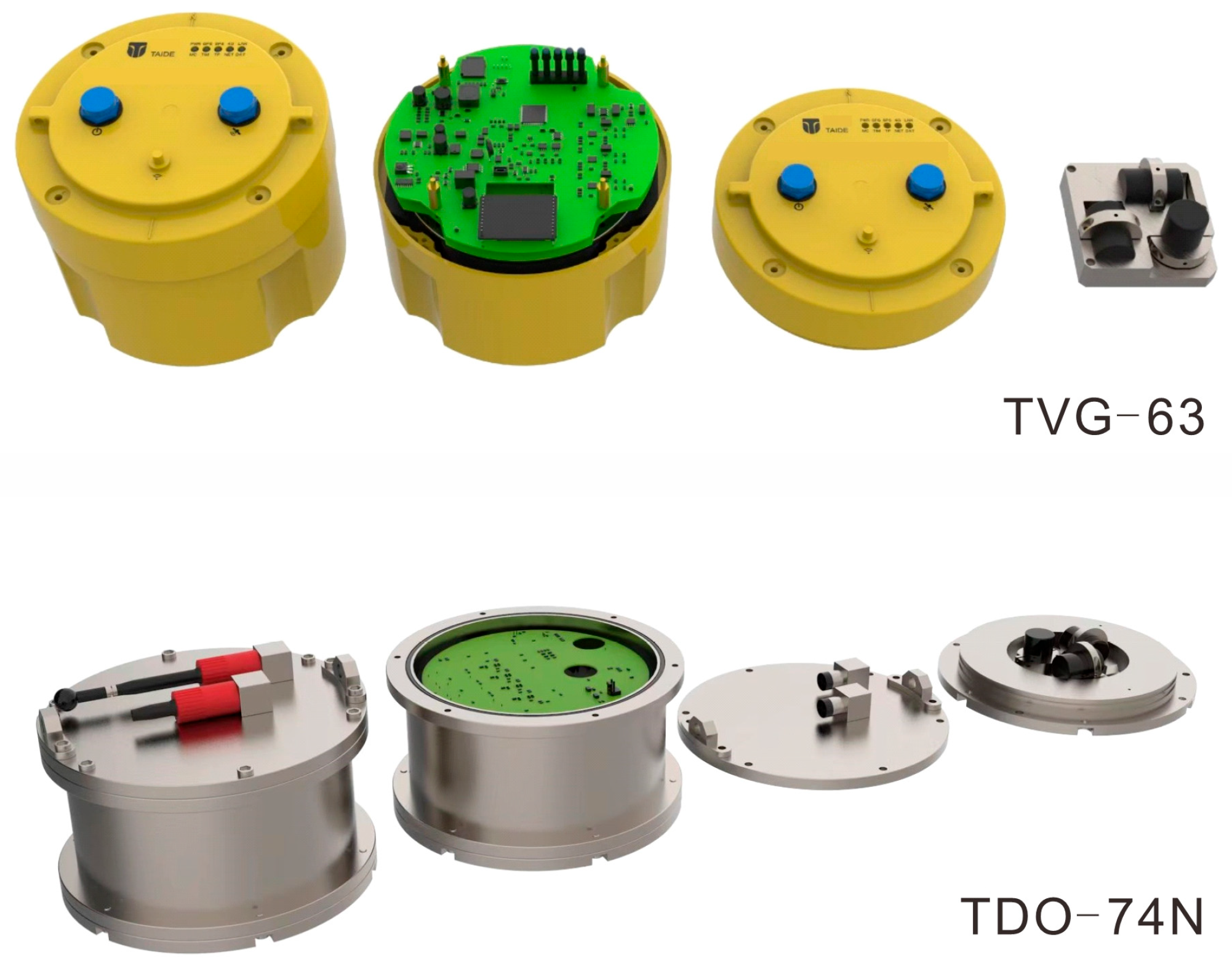
The seismic data for this study were acquired using short-period nodal seismometers, manufactured by Zhuhai Taide Enterprise Co., Ltd., Zhuhai, China, which were categorized into two types based on their deployment environment (Figure 1): Land Seismic Nodes (LSNs) deployed onshore and Ocean-Bottom Nodes (OBNs) deployed on the seafloor. Both the LSNs and the geophone component of the OBNs have an operational bandwidth of 0.1 Hz to 500 Hz. Each unit contained an integrated GNSS timing module providing absolute timing with an accuracy better than 10 μs. The LSNs were equipped with TVG-63 three-component seismometers. The OBNs employed TDO-74N four-component ocean-bottom seismometers, which integrate a three-component geophone (with the aforementioned bandwidth) and a hydrophone sensor operating over a frequency range of 1–30 kHz. All units were uniformly configured with a sampling rate of 500 Hz for this survey. Centimeter-level positioning accuracy for the LSN stations was achieved using a Trimble R9s GPS receiver operating in Real-Time Kinematic (RTK) mode. OBN positions were determined by acoustic ranging and post-processed navigation.

2.2. Data Acquisition

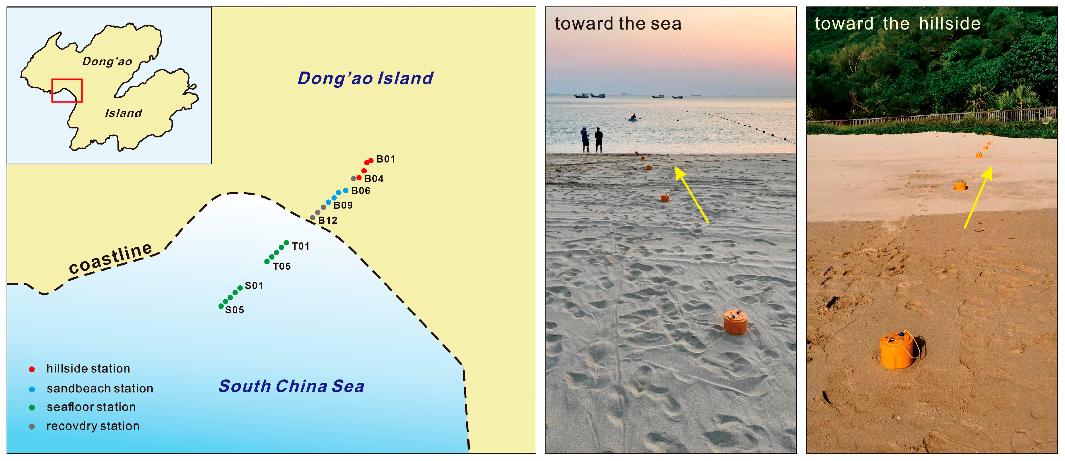
In mid-October 2022, a 142 m-long 2D survey line (from B01 to S05) was deployed along the western coastal area of Dong’ao Island using 12 LSNs and 5 OBNs across 22 station locations (Figure 2). To prevent equipment loss during nighttime high tides, the intertidal stations (B05, B10, B11, and B12) were safely recovered two hours after data acquisition commenced. Due to the limited number of OBNs (5 units), after completing nearshore observations at stations T01–T05, the instruments were relocated to deeper water positions S01–S05 to extend the submarine observation profile. The station deployment comprehensively covered three typical environments: hillside (B01-B04, with B04 adjacent to the sandbeach), sandbeach (B06–B09), and seafloor (T01–T05, S01–S05) areas, achieving approximately 24 h of continuous data acquisition from 10:00 UTC on 28 October to 09:30 UTC on 29 October. Detailed station coordinates and elevation information are provided in Table S1. For the subsequent ambient noise analysis, we utilized the vertical-component (Z) data from both LSNs and OBNs. All initial preprocessing of the raw continuous data was performed using the Seismic Analysis Code (SAC v101.6) [25].

2.3. Methods

The ambient noise data processing and inversion workflow primarily follows the methodology established by [26] employing the Frequency-Bessel (F-J) transform method to extract dispersion curves for subsequent inversion of shear-wave velocity structure. The entire procedure was carried out using our in-house F-J-VWTM Surface Wave Imaging Data Processing System, a Fortran-based platform for high-performance numerical computation. This analysis was conducted using the preprocessed vertical-component data. The procedure comprises four main stages: (1) single-station data preprocessing, (2) noise cross-correlation function computation, (3) surface wave dispersion curve extraction, and (4) shear-wave velocity structure inversion.

1.

Single-Station Data Preprocessing.

Raw vertical-component data in SEED format, recorded as hourly files at a 500 Hz sampling rate, underwent initial processing including format conversion, interpolation, concatenation, mean removal, and detrending. The data were subsequently decimated to 100 Hz. To broaden the spectral content and mitigate effects of anomalous spectral amplitudes, spectral whitening was applied [26,27]. A bandpass filter of 1–50 Hz was then applied, followed by temporal normalization [26] to minimize the influence of earthquake signals, instrumental noise, and non-stationary noise sources on the quality of noise cross-correlation functions.

2.

Cross-Correlation Function Computation.

Continuous data from each station were preprocessed (filtered to 1–50 Hz). For each station pair, these preprocessed single-station records were first temporally aligned to a common time reference. To compute the daily noise cross-correlation function (CCF), the preprocessed and aligned signal pairs were segmented into multiple time windows. The spectrum of each window was calculated, and the cross-correlation coefficients in the frequency domain were computed directly from these spectra. The coefficients from all windows were then averaged for each corresponding frequency point, yielding a single CCF for that day.

Subsequently, the daily CCFs for each station pair were linearly stacked over the entire study period using a simple arithmetic mean to enhance the signal-to-noise ratio. The resultant stacked cross-correlation functions clearly show signals on both causal and acausal components. Furthermore, the analysis indicates that Rayleigh wave group velocities in the region range approximately between 0.2 and 1.0 km/s, with the slower fundamental-mode surface waves aligning more closely with the 0.2 km/s group velocity trend.

3.

Surface Wave Dispersion Curve Extraction Using the Frequency-Bessel Transform Method.

The Frequency-Bessel transform for extracting dispersion curves from seismic noise data is defined as [28]:

$$\mathrm{I}(\mathrm{w},\mathrm{k})={\displaystyle {\int }_0^{+\infty }{\mathrm{C}}_{\mathrm{zz}}}(\mathrm{w},\mathrm{r}){\mathrm{J}}_0(\mathrm{k}\mathrm{r})\mathrm{r}\mathrm{d}\mathrm{r}$$

(1)

Here, r denotes the inter-station distance, represents the angular frequency, k is the wavenumber, C_zz(w,r) refers to the frequency-domain cross-correlation function of the vertical component, and J₀(⋅) is the zero-order Bessel function of the first kind. In practical data processing, this integral is typically approximated through numerical integration of the Green’s function at various inter-station distances r. To suppress spurious crossings in the F-J spectrum and enhance imaging quality, the Hankel function was employed in this study for the F-J transform computation [29,30,31].

The computed noise cross-correlation functions contain both causal and acausal components, which would be perfectly symmetric under ideal conditions of homogeneous noise source distribution. However, in reality, the distribution of noise sources is often heterogeneous. To mitigate this effect, the causal and acausal components are typically averaged to convert the two-sided signal into a one-sided signal (i.e., the symmetric component) [27]. This study employed the symmetric component for subsequent analysis. The Rayleigh wave group velocity dispersion curves were measured using a multiple time-frequency analysis technique [32,33].

4.

Shear-Wave Velocity Structure Inversion.

This study employed a moving station-pair approach to derive the 2D shear-wave velocity structure. A total of 214 valid station pairs were used for cross-correlation. The inversion process comprised the following steps: First, noise cross-correlation functions were computed for each adjacent station pair, and Rayleigh wave dispersion curves for individual sub-arrays were extracted using the aforementioned Frequency-Bessel transform method. Second, based on the extracted dispersion curves from each station pair, a 1D shear-wave velocity (V_s) profile beneath each station pair was obtained through inversion. The inversion was performed using an empirical formula-based [34] method implemented in the in-house F-J-VWTM Surface Wave Imaging Data Processing System. The subsurface was parameterized as a series of laterally variable, horizontal layers. The initial model was built based on available geological constraints and a preliminary 1D inversion at selected control points. During each iteration, the forward problem (dispersion-curve calculation for the current V_s model) was solved using the modal summation method. The model update was constrained by smoothing regularization to ensure geological plausibility and stability. The inversion was terminated when the misfit between observed and theoretical dispersion curves converged (typically after 10–15 iterations). Finally, the 1D shear-wave velocity structures inverted from each sub-array were treated as velocity models at the midpoint coordinates of their corresponding station pairs. These discrete 1D models were then integrated through spatial interpolation to construct a continuous 2D shear-wave velocity profile beneath the coastal zone of Dong’ao Island.

3. Analysis of Noise Characteristics

Analysis of approximately 24 h seismic recordings reveals distinct characteristics of seismic ambient noise across three different environments in the study area: hillside, sandbeach, and seafloor. While Power Spectral Density (PSD) can represent the ambient noise level during quiet periods at a station, it does not provide a comprehensive and objective assessment of the overall noise conditions and data quality. Ref. [35] introduced Probabilistic Power Spectral Densities (PPSD) as an extension of PSD, which enables evaluation of both the ambient noise level and the overall data quality at a station. This study employs the PPSD method for noise characterization. The PPSD approach processes continuous seismic waveform records directly without pre-screening, by segmenting the data into short-time sequences, repeatedly stacking them, and performing probabilistic statistics. This yields the probability distribution of signals such as seismic body waves, surface waves, and instrumental noise. Generally, larger data volumes lead to more realistic evaluation results. In contrast to PPSD, the Time Power Spectral Density (T-PSD) provides a more intuitive representation of variations in PSD values across different frequency bands over a specific time period.

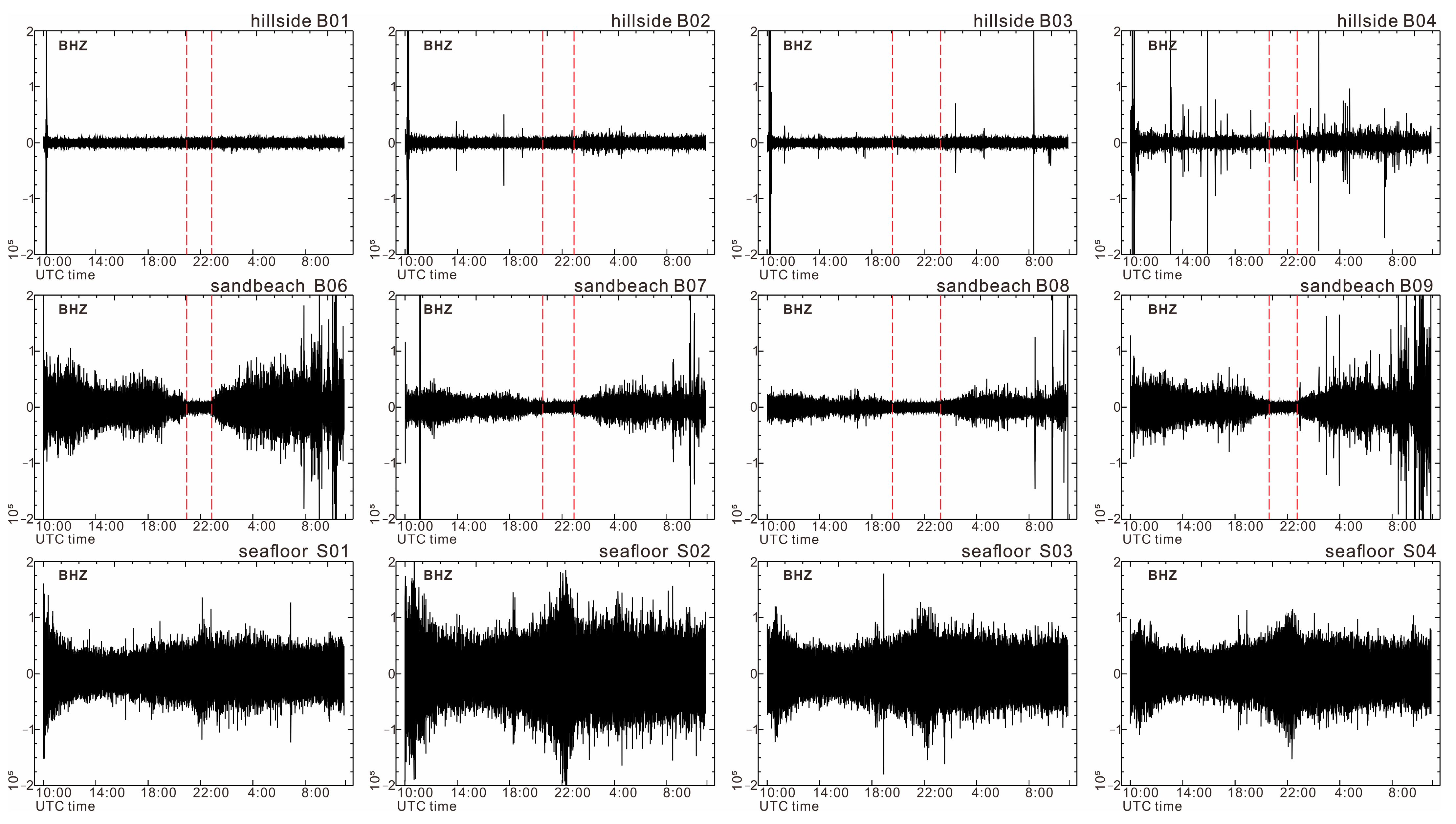
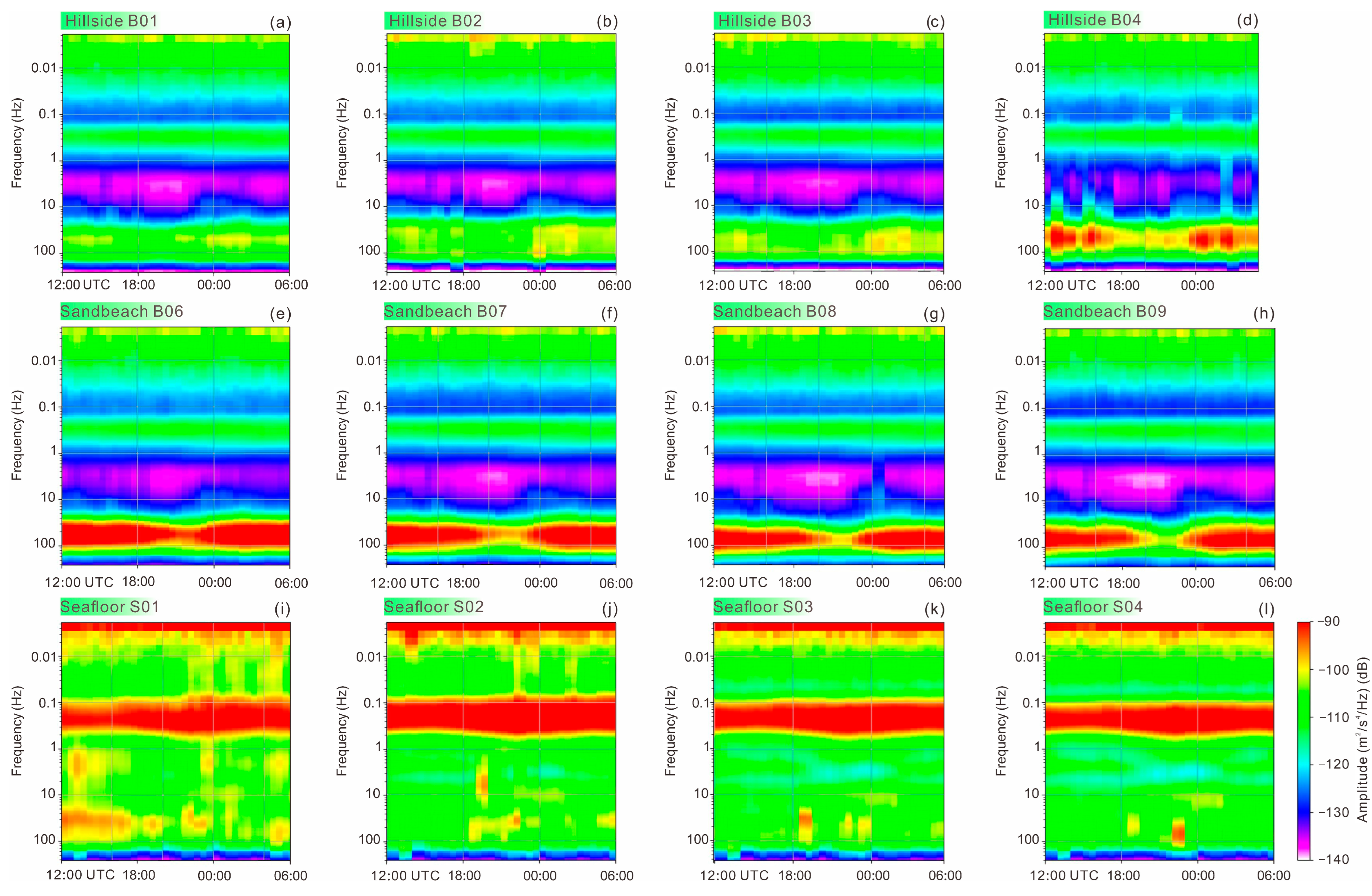
Figure 3 displays the 24 h seismic ambient noise characteristics recorded by the vertical components of LSNs and OBNs deployed in different coastal environments: hillside, sandbeach, and seafloor. The records reveal a general increasing trend in ambient noise levels from the hillside to the seafloor. Specifically, the noise levels at hillside stations (B01–B04) remain relatively stable throughout the day. In contrast, sandbeach stations (B06–B09) exhibit significantly higher noise levels during daytime compared to nighttime, with nighttime levels similar to those observed at hillside stations, indicating that anthropgenic activities primarily influence noise at beach stations during the day. Station B04, due to its proximity to the beach, shows noise characteristics similar to those of beach stations, with slightly elevated daytime noise. Seafloor stations (S01–S04), however, display a spindle-shaped noise pattern. Furthermore, the figure clearly illustrates that the ambient noise level at seafloor stations is approximately six times higher than the noise level during quiet periods on land.

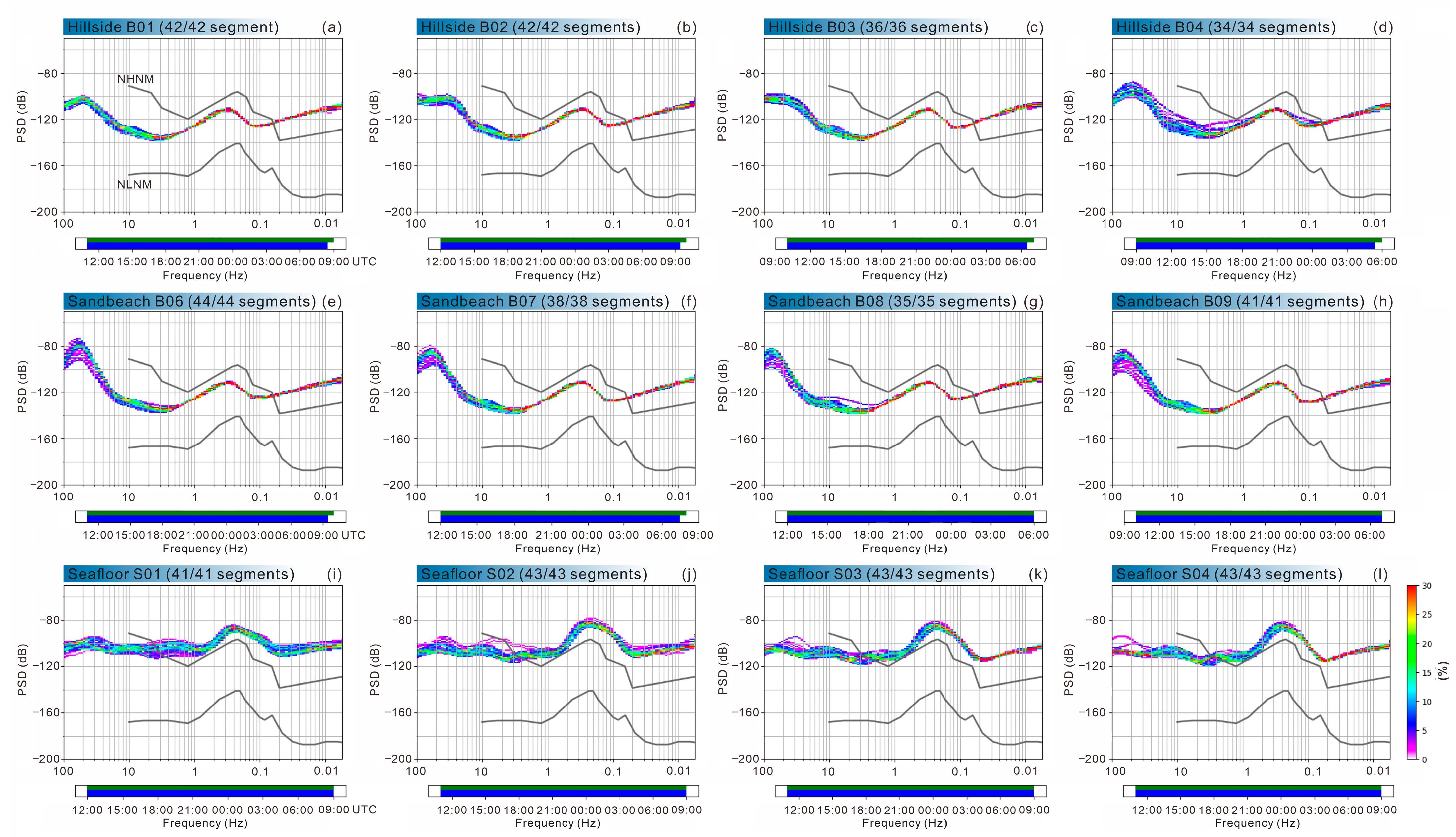
Figure 4 presents the 24 h Probabilistic Power Spectral Density (PPSD) distributions recorded by LSNs and OBNs in three distinct environments: hillside, sandbeach, and seafloor. A more concentrated PPSD distribution indicates more stable seismic ambient noise levels, whereas a more scattered distribution reflects greater noise variability. Based on the characteristic PPSD patterns, the following observations can be summarized: (1) The effective frequency range for LSNs and OBSs is from 0.1 Hz to 500 Hz. The portion of the plot beyond 10 s exceeds the instrument’s effective bandwidth and is therefore significantly distorted. (2) Within the effective frequency band, the PPSD distributions of hillside and sandbeach stations lie between the New High Noise Model (NHNM) and New Low Noise Model (NLNM) [36], with amplitudes ranging from −140 dB to −80 dB. Their overall shapes are relatively consistent with global models. In the 0.1–2.5 Hz frequency band, the probability distribution shows concentrated energy, while in the 2.5–100 Hz frequency band, the energy distribution is relatively dispersed. Sandbeach stations exhibit significantly enhanced noise energy at high frequencies, which is likely attributable to anthropogenic activities. (3) The PPSD amplitudes for seafloor stations range from −120 dB to −80 dB. Within the 7–100 Hz frequency band, their PPSD distributions generally fall between the NLNM and NHNM, lying closer to the NHNM and showing relatively scattered probability densities. At frequencies below this band, the PPSD values rise above the NHNM, reflecting elevated ambient-noise levels across much of the observable frequency range in the submarine environment. (4) In all three environments, high-frequency seismic ambient noise signals with frequencies above 1Hz are both abundant and stable.

Figure 5 displays the T-PSD for seismic ambient noise recorded by the vertical component of LSNs and OBNs. The main characteristics are as follows: (1) Distinct T-PSD patterns are observed across the three environments, with seafloor stations exhibiting significantly higher overall ambient noise energy compared to land stations. (2) At seafloor stations, the ambient noise energy is predominantly concentrated in the 0.1–0.5 Hz frequency band (secondary microseisms). A secondary energy peak is consistently present in the 2–100 Hz band. While such high frequencies are typically associated with anthropogenic sources on land, their presence on the seafloor is likely influenced by a combination of hydrodynamic noise (waves/currents), vibrations from distant ship traffic propagating through the water column and seabed, and potential activity from nearby marine operations. (3) At stations located above the waterline (hillside B01–B04 and sandbeach B06–B09), the intensity of high-frequency (>1 Hz) noise shows a clear diurnal pattern that correlates with human activity. A pronounced reduction in energy is observed during local nighttime hours (approximately midnight to 06:00 a.m. Beijing time), coinciding with periods of minimal anthropogenic disturbance. In contrast, the high-frequency noise at seafloor stations exhibits a weaker correlation with this diurnal cycle, though its average energy level remains intermediate between that recorded at hillside and sandbeach stations. (4) The timing of onset and cessation of elevated high-frequency (>1 Hz) noise varies among stations and is influenced by station location. Notably, the distribution of high-frequency energy becomes more uniform with increasing proximity to the sea, reflecting a blending of terrestrial and marine noise sources.

4. Results

4.1. Dispersion Curve Measurement

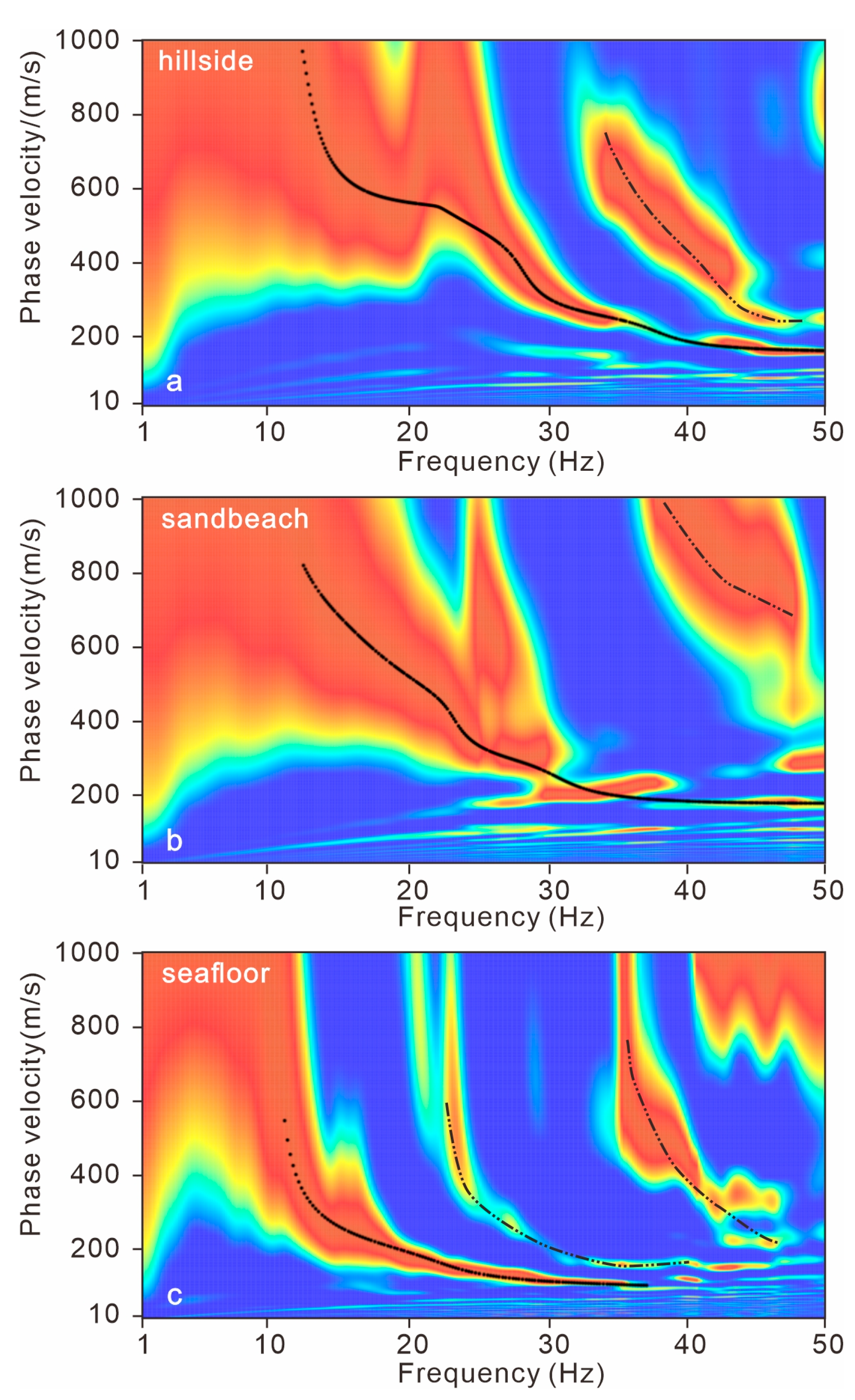
Based on the previously described Frequency-Bessel (F-J) transform method, Rayleigh wave dispersion curves were extracted from the three distinct environments: hillside, sandbeach, and seafloor (Figure 6). The results demonstrate that for both hillside and sandbeach stations, the dispersion energy is relatively scattered at frequencies below approximately 15 Hz, making it difficult to reliably extract stable dispersion curves. Similarly, seafloor stations present challenges in extracting usable signals below about 10 Hz. In contrast, the seafloor stations exhibit more concentrated energy distribution for both fundamental and higher modes. Within the frequency ranges of 30–50 Hz (hillside) and 35–50 Hz (sandbeach), signals that could be associated with higher modes appear scattered and morphologically poorly defined, indicating challenges in resolving clear dispersion trends at these sites. n contrast, seafloor stations exhibit a clear and continuous fundamental mode. Additionally, a distinct second-order mode is observable within the 20–45 Hz range at seafloor stations, reflecting a more coherent and higher-quality ambient noise wavefield in the marine environment.

4.2. Shallow S-Wave Velocity Structure of Dong’ao Island Coastal Zone

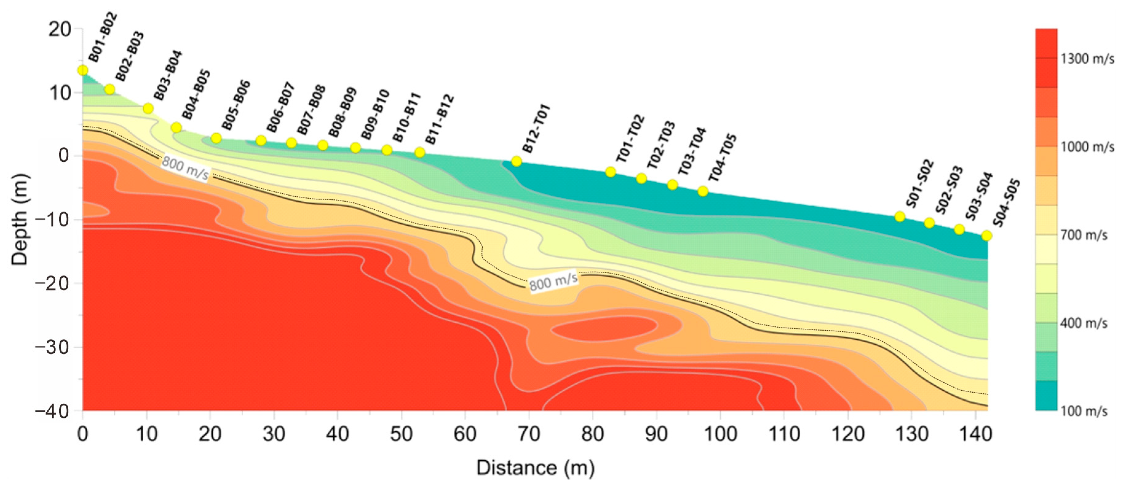
Cross-correlation calculations were performed for all possible pairs among the 22 stations. After excluding station pairs from which reliable dispersion curves could not be extracted, a two-dimensional S-wave velocity profile beneath the survey line was constructed through interpolation of the remaining 20 one-dimensional S-wave velocity models (Figure 7). It should be noted that the yellow circles in the figure do not represent actual station locations, but rather the projected midpoints of the respective cross-correlated station pairs. With reference to the ASCE/SEI 7–10 standard [37] and the regional study by Chen et al. [38], layers with shear-wave velocities exceeding 760 m/s were defined as bedrock. Accordingly, the 760 m/s contour was used to delineate the bedrock surface in this study. The estimated sediment thicknesses beneath the land station B10 and the seafloor station S03 are 10.10 m and 25.80 m, respectively. The sediment thicknesses presented here were estimated directly from this 2D profile by measuring the vertical distance from the surface (or seafloor) to the 760 m/s contour.

4.3. Comparison with HVSR Results

In recent years, the Horizontal-to-Vertical Spectral Ratio (HVSR) method has been widely applied in sediment thickness estimation [39,40,41,42,43]. This technique analyzes the spectral ratio between the horizontal and vertical components of ambient noise signals to identify the fundamental resonance frequency (f₀) of the sediment layer. The relationship between f₀, sediment thickness (h), and the average shear-wave velocity (V_s) is expressed as:

h = V_s/4f₀

(2)

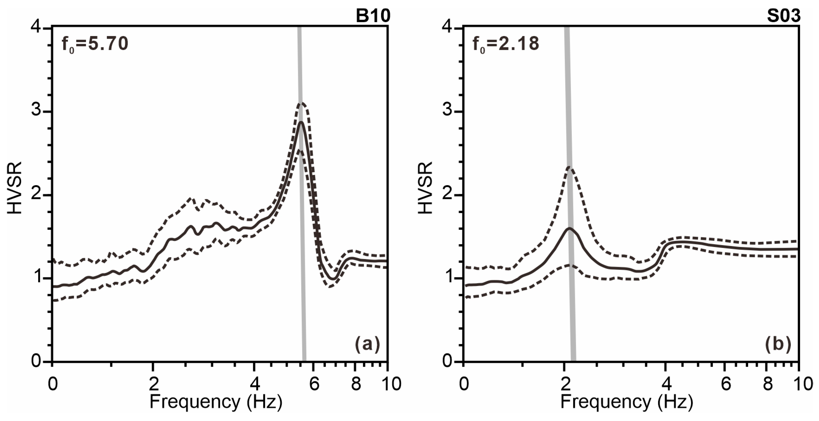
In this study, the frequency value exhibiting the maximum amplitude with a clear peak shape within the analyzed bandwidth was selected as the fundamental resonance frequency (f₀), interpreted to correspond to the sediment-bedrock interface. The identified f₀ values for stations B10 and S03 were 5.70 Hz and 2.18 Hz, respectively (Figure 8). The coastal zone of Dong’ao Island is predominantly characterized by soft marine sediments. The stratigraphic sequence above the bedrock, from top to bottom, consists of a silt layer, a silty clay layer, a residual soil layer, and a completely weathered granite layer. For subsequent site response analysis, an average shear-wave velocity of V_s = 220 m/s was adopted for the sediment column above the defined bedrock. This value is not a direct inversion output but a representative engineering estimate. It was selected because it falls within the typical V_s30 range (200–250 m/s) for similar coastal sedimentary environments in the region [37], and is consistent with the velocity gradient (primarily <300 m/s) observed in the shallow part of our derived model (Figure 7). This empirical choice is acknowledged as a limitation, and future work with borehole constraints is recommended for more precise calibration. Using formula (2), the sediment thicknesses beneath stations B10 and S03 were estimated to be approximately 9.64 m and 25.23 m, respectively.

The estimates of bedrock depth for the two stations derived from the F-J method are 10.10 m (B10) and 25.80 m (S03), while those from the HVSR method are 9.64 m (B10) and 25.23 m (S03). The results from both methods show good consistency, with relative errors for both stations being within 5%. This close agreement demonstrates the reliability of the F-J method for estimating sediment thickness in coastal zones. However, phenomena such as multiple peaks and spurious peaks can still be observed in the HVSR curve morphology (Figure 8), which may interfere with the accurate estimation of sediment thickness. In addition to the previously mentioned factors, including multiple wave impedance interfaces, anthropogenic vibration interference, thick silt layers, and loose sand layers, the coupling condition between the OBNs and the seafloor is also a critical influencing factor. Zhou et al. [43] systematically analyzed the characteristics of spectral ratio curves by deploying multiple sets of OBNs on the seafloor in different configurations. Their results demonstrated that the deployment method significantly affects the identification of the peak frequency: the spectral ratio curves obtained from seismometers placed in sand-filled boxes showed significantly clearer peaks compared to those from boxes without sand or instruments placed directly on the seafloor. Furthermore, seafloor topography also has a certain influence on the spectral ratio characteristics of the stations. Therefore, when applying the HVSR method for marine site effect studies, it is necessary to comprehensively consider the influence of topographic conditions and instrument deployment methods on the results.

In this survey, the OBNs were deployed using a rope-string connection method, released one by one along the survey line with the aid of a kayak. Although the release process was controlled as much as possible, it was difficult to ensure ideal coupling between the OBNs and the seafloor in some areas where the water depth reached approximately 13 m, creating the possibility of instrument tilt or overturning, which consequently affected data quality to some extent. To enhance the reliability of future observational data, it is recommended to optimize the deployment scheme: in areas above the waterline, seismometers can be buried directly in the ground surface; for shallow-water areas, divers could be arranged to perform underwater burial operations at designated locations to fully ensure the coupling quality between the OBNs and the sediments.

5. Discussion

This study successfully obtained the shallow shear-wave velocity structure from the hillside to the seafloor in the coastal zone of Dong’ao Island, Zhuhai, using LSNs and OBNs and the seismic ambient noise method. The results, mutually validated with those from the HVSR method, demonstrate the feasibility of this technique in land–sea transition zones. However, based on the experience and findings from this experiment, several key issues warrant further discussion

1.

Applicability and Potential of the Ambient Noise Method in Coastal Zones

The results of this study indicate that seismic ambient noise imaging exhibits unique applicability and significant potential for shallow subsurface detection in coastal zones. Its core advantage lies in utilizing persistent natural and cultural noise in the environment as the signal source, thereby overcoming the physical obstacles and economic costs associated with active-source methods related to energy generation and signal reception at the land-water interface. The flexible deployment of LSNs and OBNs enables seamless coverage of complex environments. Noise analysis across different settings confirms that, despite variations in energy and spectral characteristics, the stable and abundant high-frequency (>1 Hz) noise signals guarantee the extraction of high-quality dispersion curves. Particularly important is the high consistency in bedrock depth estimates between the F-J method and the HVSR method, which are based on different physical principles. In the absence of borehole data, this provides effective cross-validation, confirming not only the method’s reliability but also highlighting its practical value for preliminary surveys and rapid screening in coastal zones.

2.

Data Quality and Analysis of Inversion Uncertainty

All geophysical inversions suffer from non-uniqueness, and data quality is the primary factor constraining the accuracy of the inversion results. The quality of the extracted dispersion curves directly constrains the inversion. At onshore sites, the fundamental-mode dispersion energy is scattered at lower frequencies, and any identifiable higher-mode signals are diffuse (Figure 6). This may be related to shallow subsurface heterogeneity, local anthropogenic disturbances, and insufficient sampling of high-frequency signals due to limited station spacing, resulting in weaker constraints on the shallow structure. In contrast, the fundamental-mode curves from seafloor stations are more continuous and stable. The additional observation of a clearer second-order mode at these stations further attests to the superior wavefield coherence and data quality in the homogeneous marine setting, which facilitated a more reliable inversion. Furthermore, the coupling condition of OBNs is a key uncertainty factor affecting data quality. The deployment method used in this study may have caused instrument tilt or poor coupling, subsequently affecting the HVSR curve morphology (e.g., causing multiple peaks) and the calculation of cross-correlation functions. Therefore, future work must prioritize improving instrument deployment techniques to reduce errors and inversion uncertainties introduced by coupling issues.

3.

Technical Optimization and Future Research Directions

To enhance the accuracy and resolution of ambient noise imaging in coastal zones, future research should focus on technical optimization from several aspects. First, promoting joint active and passive source surveys is a key pathway to overcoming the resolution limitations in the very shallow subsurface. Incorporating active sources, such as high-frequency vibrators, can compensate for the lack of high-frequency energy in passive noise, enabling the acquisition of more complete and reliable dispersion curves through joint inversion. Second, establishing a multi-method cross-validation framework is crucial. In particular, the direct and high-resolution stratigraphic information provided by Cone Penetration Testing (CPT) can serve as critical “ground truth” validation data. In the absence of “hard” data from drilling, CPT profiles, along with other geophysical methods like resistivity and transient electromagnetic surveys, should be integrated. The continuous lithological and mechanical parameters from CPT can effectively calibrate shear-wave velocity models derived from surface wave inversion, reducing uncertainties in layer boundaries and velocity values. Leveraging the complementary relationships between different geophysical parameters can jointly constrain and validate the velocity model, reducing inversion non-uniqueness. Finally, conducting systematic experiments on acquisition parameters is fundamental for standardizing and operationalizing this method. Future work should design comparative experiments involving different station spacings, recording durations, and sampling rates tailored to specific geological targets. This will help establish optimal operational procedures for ambient noise surveys in coastal zones, thereby maximizing the scientific value and application benefits of the data within limited budgets.

6. Conclusions

Based on the seismic ambient noise data acquired from the western coastal area of Dong’ao Island in Zhuhai, along with systematic signal processing, dispersion curve extraction, and inversion analysis, this study draws the following main conclusions:

• The characteristics of seismic ambient noise in different coastal environments have been clearly identified. Seafloor stations exhibit the strongest ambient noise energy, approximately six times greater than that during quiet periods on land. The predominant noise energy is concentrated in the 0.1–0.5 Hz frequency band (secondary microseisms) and the 2–100 Hz frequency band (high-frequency cultural noise). Despite spatiotemporal variations in noise levels, all stations recorded abundant and stable high-frequency noise (>1 Hz), confirming the data foundation for utilizing ambient noise in detecting shallow subsurface structures in coastal zones.
• High-quality Rayleigh wave dispersion curves were successfully extracted from the ambient noise using the Frequency-Bessel (F-J) transform method, enabling the inversion of a continuous 2D shear-wave velocity structure beneath the coastal zone. The results show that the sediment thickness gradually increases from approximately 10.10 m at the land station (B10) to about 25.80 m at the seafloor station (S03), illustrating a continuous lateral variation in the subsurface structure.
• Comparative validation with the Horizontal-to-Vertical Spectral Ratio (HVSR) method demonstrates a high level of agreement in the estimated bedrock depths between the two methods. This consistency, derived from different physical principles, provides cross-validation of the feasibility and reliability of the seismic ambient noise method for detecting shallow stratigraphic structures and the bedrock surface in complex coastal environments.
• This study successfully achieved seamless deployment and joint observation of LSNs and OBNs from land to sea, confirming that seismic ambient noise imaging technology is an effective solution for eliminating “exploration gaps” in coastal zones and achieving integrated land–sea shallow subsurface structural detection. The method shows broad application prospects in fields such as engineering geological surveys, marine site characterization, and geohazard assessment.
• The study also identified limitations in the current method when applied in marine environments, such as the influence of ocean-bottom seismometer coupling conditions on data quality. Accordingly, targeted technical recommendations are proposed, including improved instrument deployment schemes, the systematic incorporation of in situ tests like CPT for calibration, and the implementation of joint active and passive source surveys, providing clear directions for future research.

References

1. Huang, C.; Liu, S.; Long, J.Q.; Zhang, C.R.; Xiao, B.; Wang, D.C.; Wei, C.L.; Wang, R.; Yan, L.; Hu, X.; et al. Application of ambient noise tomography to coastal granite islands: A case study of Wuzhizhou Island in Hainan, China. Appl. Geophys. 2025, 22, 1326–1340. [Google Scholar] [CrossRef]
2. Duan, X.; Zhang, Z.; Ding, H.; Han, M.; Gu, Z. Multi-Scale Refraction Tomography Constrained by Geostatistical Information Method and its Application in Bohai Bay. In Proceedings of the International Petroleum Technology Conference, Kuala Lumpur, Malaysia, 18–20 February 2025. [Google Scholar]
3. Dale, B.; Maha, K.; Dominic, L.; Vanessa, B.; James, S.; Mostafa, M.; Ekramy, F.; Mohamed, R. Solving East Nile Delta’s imaging challenges through new ocean-bottom-node acquisition and advanced imaging. Lead. Edge 2024, 43, 615–622. [Google Scholar]
4. Liu, C.N.; Lin, F.C.; Huang, H.H.; Wang, Y.; Gkogkas, K. Multimode ambient noise double-beamforming tomography with a dense linear array: Revealing accretionary wedge architecture across Central Taiwan. Geophys. J. Int. 2024, 239, 467–477. [Google Scholar] [CrossRef]
5. Liu, X.; Hu, K.T.; Qian, R.Y.; Zhao, S.A.; Zhang, J.; Ling, J.Y.; Ma, Z.N.; Wu, Z.Y.; Huang, Y.H.; Meng, Y.Q.; et al. 3D high-density ambient noise imaging of the Nankou-Sunhe buried active fault in Beijing. Eng. Geol. 2025, 345, 0013–7952. [Google Scholar] [CrossRef]
6. Le, T.; Xinding, F. Application of six-component ambient seismic noise data for high-resolution imaging of lateral heterogeneities. Geophys. J. Int. 2023, 232, 1756–1784. [Google Scholar]
7. Chen, L.; Xue, M.; Phon, L.K.; Yang, T. Rayleigh wave group velocity tomography in South China Sea and its geodynamic implications. Acta Seismol. Sin. 2012, 34, 754–772. [Google Scholar]
8. Cao, X.L.; Zhu, J.S.; Zhao, L.F.; Cao, J.M.; Hong, X.H. 3D S-wave velocity structure of crust and upper mantle in South China Sea and its adjacent regions by surface wave waveform inversion. Acta Seismol. Sin. 2001, 23, 113–124. [Google Scholar]
9. Schuster, G.T.; Li, J.; Lu, K.; Metwally, A.; Altheyab, A.; Hanafy, S. Opportunities and pitfalls in surface-wave interpretation. Interpretation 2017, 5, 131–141. [Google Scholar] [CrossRef]
10. Kang, S.Y.; Kim, K.H. Bedrock Depth Variations and Their Applications to identify Blind Faults in the Pohang area using the Horizontal-to-Vertical Spectral Ratio (HVSR). J. Korean Earth Sci. Soc. 2022, 43, 188–198. [Google Scholar] [CrossRef]
11. Picozzi, M.; Parolai, S.; Bindi, D.; Strollo, A. Characterization of shallow geology by high-frequency seismic noise tomography. Geophys. J. Int. 2009, 176, 164–174. [Google Scholar] [CrossRef]
12. Lewińska, P.; Matuła, R.; Dyczko, A.; Nykiel, G. Integration of thermal digital 3d model and a masw (multichannel analysis of surface wave) as a means of improving monitoring of spoil tip stability. In Proceedings of the 2017 Baltic Geodetic Congress (BGC Geomatics), Gdansk, Poland, 22–25 June 2017; pp. 232–236. [Google Scholar]
13. Mahvelati, S.; Coe, J. Horizontal-to-Vertical Spectral Ratio (HVSR) Analysis of the Martian Passive Seismic Data from the InSight Mission. In Earth and Space; ASCE Library: Reston, VA, USA, 2021. [Google Scholar]
14. Larose, E.; Khan, A.; Nakamura, Y.; Campillo, M. Lunar subsurface investigated from correlation of seismic noise. Geophys. Res. Lett. 2005, 32, L16201. [Google Scholar] [CrossRef]
15. Sivaram, K.; Mahesh, P.; Rai, S.S. Stability assessment and quantitative evaluation of H/V spectral ratios for site response studies in Kumaon Himalaya, India using ambient noise recorded by a broadband seismograph network. Pure Appl. Geophys. 2012, 169, 1801–1820. [Google Scholar] [CrossRef]
16. Xiong, Y.L.; Gao, J.H.; Peng, J. Research and application of natural source surface wave method on barrier lake deposits. Chin. J. Eng. Geophys. 2022, 19, 149–154. [Google Scholar]
17. Wu, Q.B.; Pan, Z.Q.; Chen, J.Y.; Mubarak; Hani. Detection of shallow basalt 3D distribution using transient Rayleigh wave method: A case study of Sabkhah Ad Dumathah area, Saudi Arabia. Prog. Geophys. 2019, 34, 1938–1944. [Google Scholar]
18. Xu, P.F.; Li, C.J.; Ling, S.Q.; Zhang, Y.B.; Hou, C.; Sun, Y.J. Detection of collapse columns in coal mines using microtremor survey method. Chin. J. Geophys. 2009, 52, 1923–1930. [Google Scholar]
19. Mainsant, G.; Larose, E.; Brönnimann, C.; Jongmans, D.; Michoud, C.; Jaboyedoff, M. Ambient seismic noise monitoring of a clay landslide: Toward failure prediction. J. Geophys. Res. Earth Surf. 2012, 117. [Google Scholar] [CrossRef]
20. Wang, J.; Zheng, J.; Sun, Y.; Xu, L.; He, Y.; Gong, J.; Wang, C.; Zhan, X.; Wan, Y.; Ren, W. Characteristics of Ambient Seismic Noise Recorded at Offshore Wind Turbine Platform Monitoring Stations. Earthq. Res. Adv. 2025, 100440. [Google Scholar] [CrossRef]
21. Obermann, A.; Planès, T.; Larose, E.; Campillo, M. Imaging preeruptive and coeruptive structural and mechanical changes of a volcano with ambient seismic noise. J. Geophys. Res. Solid Earth. 2013, 118, 6285–6294. [Google Scholar] [CrossRef]
22. Cicconi, G.; Dagnino, I.; Eva, C. Comparative spectra of microseisms and swell in the Ligurian Sea. Dev. Solid Earth Geophys. 1983, 15, 237–241. [Google Scholar]
23. Hasselmann, K. A statistical analysis of the generation of microseisms. Rev. Geophys. 1963, 1, 177–210. [Google Scholar] [CrossRef]
24. Longuet-Higgins, M.S. A Theory of the Origin of Microseisms. Philos. Trans. R. Soc. Lond. 1950, 243, 1–35. [Google Scholar] [CrossRef]
25. Goldstein, P.; Snoke, A. SAC availability for the IRIS community. Off. Sci. Tech. Inf. Tech. Rep. 2005, 7. Available online: https://www.semanticscholar.org/paper/SAC-Availability-for-the-IRIS-Community-Goldstein-Snoke/527e67c5fee6f2da5e64a183fee3337fb5893468#citing-papers (accessed on 29 January 2026).
26. Bensen, G.D.; Ritzwoller, M.H.; Barmin, M.P.; Levshin, A.L.; Lin, F.; Moschetti, M.P.; Shapiro, N.M.; Yang, Y. Processing seismic ambient noise data to obtain reliable broad-band surface wave dispersion measurements. Geophys. J. R. Astron. Soc. 2010, 169, 1239–1260. [Google Scholar] [CrossRef]
27. Fang, L.H.; Wu, J.P.; Lü, Z.Y. Rayleigh surface wave group velocity tomography based on noise in North China. Chin. J. Geophys. 2009, 52, 9. [Google Scholar]
28. Wang, J.N.; Wu, G.X.; Chen, X.F. Frequency-Bessel transform method for effective imaging of higher-mode Raleigh dispersion curves from ambient seismic noise data. J. Geophys. Res. Solid Earth 2019, 124, 3708–3723. [Google Scholar] [CrossRef]
29. Forbriger, T. Inversion of shallow-seismic wavefields: I. wavefield transformation. Geophys. J. Int. 2003, 153, 719–734. [Google Scholar] [CrossRef]
30. Xi, C.Q.; Xia, J.H.; Mi, B.B.; Dai, T.Y.; Liu, Y.; Ning, L. Modified frequency-Besseltransform method for dispersion imaging of Rayleigh waves fromambient seismic noise. Geophys. J. Int. 2021, 225, 1271–1280. [Google Scholar] [CrossRef]
31. Zhou, J.; Chen, X. Removal of crossed artifacts from multimodaldispersion curves with modified Frequency-Bessel method. Bull. Seismol. Soc. Am. 2022, 112, 143–152. [Google Scholar] [CrossRef]
32. Dziewonski, A.; Bloch, S.; Landisman, M. A Technique for the Analysis of Transient Seismic Signals. Bull. Seismol. Soc. Am. 1969, 59, 427–444. [Google Scholar] [CrossRef]
33. Levshin, A.; Ratnikova, L.I.; Berger, J. Peculiarities of surface wave propagation across Central Asia. Bull. Seismol. Soc. Am. 1992, 82, 2464–2493. [Google Scholar] [CrossRef]
34. Ling, S.Q.; Miwa, S. The evaluation of soil structures by Surface Wave Prospecting Method and Microtreror Survey Method-2004 Mid Nigata Prefecture Earthquake. In A New Technique on Engineering Geophysical Method; Liu, Y.Z., Ed.; Geological Publishing House: Beijing, China, 2006; pp. 80–85. [Google Scholar]
35. Beyreuther, M.; Barsch, R.; Krischer, L.; Megies, T.; Behr, Y.; Wassermann, J. Obspy: A python toolbox for seismology. GeoScienceWorld 2010, 81, 530–533. [Google Scholar] [CrossRef]
36. Peterson, J. Observations and Modeling of Seismic Background Noise; U.S. Geological Survey Open File Report; US Geological Survey: Reston, VA, USA, 1993; pp. 93–322. [Google Scholar]
37. ASCE. Minimum Design Loads for Buildings and Other Structures (ASCE/SEI 7–10). Am. Soc. Civ. Eng. 2014, 559, 996. [Google Scholar]
38. Chen, T.; Chen, L.W.; Guo, T.T.; Liu, G. Correlation of site average shear-wave velocity and the fundamental frequency. Earthq. Eng. Eng. Dyn. 2022, 42, 190–199. [Google Scholar]
39. Nakamura, Y. A method for dynamic characteristics estimation of subsurface using microtremor on the ground surfac. Q. Rep. RTRI 1989, 30, 25–33. [Google Scholar]
40. Picotti, S.; Francese, R.; Giorgi, M.; Pettenati, F.; José, M.C. Estimation of glacier thicknesses and basal properties using the horizontal-to-vertical component spectral ratio (HVSR) technique from passive seismic data. J. Glaciol. 2017, 63, 229–248. [Google Scholar] [CrossRef]
41. Zong, J.Y.; Sun, X.L.; Zhang, P. Site effect and earthquake disaster characteristics in Guangzhou area from horizontal-to-vertical spectral ratio (HVSR) method. Seismol. Geol. 2020, 42, 628–639. [Google Scholar]
42. Xiong, C.; Ye, X.W.; Zhang, Y.X.; Lü, Z.Y.; Wang, L.Y. Application of noise HVSR method in OBS detection: A case study of OBS array off the Pearl River Estuary. Chin. J. Geophys. 2023, 66, 2951–2960. [Google Scholar]
43. Zhou, X.T.; Hu, J.J.; Tan, J.Y.; Cui, X. The Study of Site Effect of DONET1 Offshore Ground Motions Based on HVSR. Technol. Earthq. Disaster Prev. 2021, 16, 105–115. [Google Scholar]
Figure 1. Structural schematic diagrams for TVG-63 and TDO-74N.
Jmse 14 00334 g001
Figure 2. Schematic diagram of the study area and distribution of LSNs and OBNs. The red box indicates the location of the study area. The yellow arrows represent toward the sea and toward the hillside, respectively.
Jmse 14 00334 g002
Figure 3. Vertical-component seismic ambient noise recorded over approximately 24 h from 10:00 UTC, 28 October to 09:30 UTC, 29 October, with the red dashed box indicating the period when noise levels at hillside and sandbeach stations were similar during nighttime.
Jmse 14 00334 g003
Figure 4. Vertical component seismic ambient noise PPSD distribution in 24 h. The NHNM and NLNM are shown as reference curves. At the bottom of each panel, the green rectangular bar indicates all available data, while the blue portion represents the data subset actually used in the PPSD computation. (ad) represent hillslope stations, (eh) represent sandbeach stations, (il) represent seafloor stations.
Jmse 14 00334 g004
Figure 5. Vertical component seismic ambient noise T-PSD variations in 24 h. The horizontal axis represents time in UTC, with all times starting from 12:00 UTC. (ad) represent hillslope stations, (eh) represent sandbeach stations, (il) represent seafloor stations.
Jmse 14 00334 g005
Figure 6. Dispersion curves from LSNs and OBNs at different locations in the coastal zone. (a) Frequency-phase velocity spectrum for stations B01–B04; (b) Frequency-phase velocity spectrum for stations B06–B09; (c) Frequency-phase velocity spectrum for stations S01–S05. The black lines represent the manually picked fundamental-mode dispersion curves. The black dashed lines represent the theoretical dispersion curves for different modes.
Jmse 14 00334 g006
Figure 7. Two-dimensional shear-wave velocity profile.
Jmse 14 00334 g007
Figure 8. Representative HVSR curve characteristics in the coastal zone. (a) represents B10 station, (b) represent S03 station. The solid line represents the average HVSR, while the dashed line represents the range of HVSR across different time windows.
Jmse 14 00334 g008
Disclaimer/Publisher’s Note: The statements, opinions and data contained in all publications are solely those of the individual author(s) and contributor(s) and not of MDPI and/or the editor(s). MDPI and/or the editor(s) disclaim responsibility for any injury to people or property resulting from any ideas, methods, instructions or products referred to in the content.