A Novel ROA-Optimized CNN-BiGRU Hybrid Network with an Attention Mechanism for Ship Fuel Consumption Prediction

Abstract

Optimizing ship energy efficiency and advancing the green transition of the shipping industry depend on an accurate model for predicting ship fuel consumption (FC). This study builds a hybrid prediction model that combines a Convolutional Neural Network (CNN), Bidirectional Gated Recurrent Unit (BiGRU), and an attention mechanism using operational data from ships. The model is tuned using the Red Kite Optimization Algorithm (ROA). First, correlations between ship navigational environmental data and operational data are analyzed, and cluster analysis is performed to select suitable input features. Subsequently, the ship FC prediction model based on ROA-CNN-BiGRU-Attention (RCGA) is developed. A case study shows that the RCGA model reaches a root mean square error (RMSE) as low as 0.0205 and an R² value as high as 0.9330, demonstrating strong performance in dynamic shipping scenarios, with advantages in handling temporal dependencies and complex operational patterns. Moreover, the model exhibits reasonable robustness, providing some support for ship energy efficiency optimization and assisting the shipping industry in advancing low-carbon development and sustainable green transition.

1. Introduction

1.1. Backgrounds

As a cornerstone of global trade, the shipping industry is responsible for over 80% of world trade volume, serving as a vital force driving global economic integration [1]. However, the prosperity of the industry also introduces severe environmental challenges. Due to its heavy reliance on fossil fuels, the greenhouse gas emissions generated by the shipping sector have become a global concern. According to the International Maritime Organization (IMO), global shipping carbon dioxide emissions reached 1.076 billion tons in 2018, accounting for approximately 2.89% of the global emissions. Global CO₂ emissions from shipping are projected to reach 90–130% of 2008 levels by 2050 [2].

In response to global climate change, the IMO has adopted a revised strategy aiming for net-zero greenhouse gas (GHG) emissions around 2050, which requires the shipping industry to implement a dual approach focused on carbon reduction and energy efficiency improvement. In addition to adopting alternative marine fuels—such as liquefied natural gas (LNG), methanol, hydrogen, and ammonia—to reduce CO₂ emissions [3], improving ship energy efficiency and reducing FC have become central to the sustainable development of the shipping industry [4,5].

In 2009, the official guidelines for the Energy Efficiency Operational Indicator (EEOI) released by the IMO clearly stated that the EEOI serves the functions of evaluating the operational energy efficiency of ships and identifying the potential for energy efficiency optimization [6]. In 2013, the Ship Energy Efficiency Management Plan (SEEMP) guidelines issued by the IMO explicitly listed “fuel consumption monitoring and prediction” as a core component of ship energy efficiency management, noting that accurate FC prediction can support operations such as speed optimization and route planning [7]. A precise and reliable ship FC prediction model can offer critical data support for operational measures such as ship speed optimization, sailing route planning, and trim optimization, thereby maximizing fuel savings while ensuring the fulfillment of voyage tasks [8]. The key approach for achieving low-carbon shipping is ship energy efficiency optimization, which involves adjusting operational and navigational factors to minimize ship FC and CO₂ emissions.

The ship energy efficiency optimization requires an accurate FC model as a basis for evaluating the energy-saving effects of different optimization strategies. Yan et al. [9] developed a ship FC prediction model using the Random Forest method based on voyage report data from a dry bulk carrier. The model achieved fuel savings ranging from 2% to 7%, significantly reducing carbon dioxide emissions. Li et al. [10] first established ship FC prediction and shaft speed prediction models, both with relative errors of less than 0.9%. Subsequently, they proposed an iterative algorithm for weather-loaded speed optimization based on route segmentation that considers actual weather conditions. The results demonstrated that the optimized ship FC achieved savings ranging from 2.3% to 5.2%, indicating significant fuel economy. Considering the coupling effects among route, speed, trim, and various environmental variables, Li et al. [11] employed an improved Long Short-Term Memory (LSTM) method to establish a ship energy consumption prediction model based on a Genetic Algorithm (GA) and subsequently developed a cooperative optimization method using the Non-dominated Sorting Genetic Algorithm III (NSGA-III). The results demonstrated that this cooperative optimization strategy could achieve fuel savings of up to 4.54%, indicating a significant optimization effect. To evaluate the synergistic effects of navigation speed, displacement, hull trim angle, and weather and sea conditions on ship fuel efficiency, Du et al. [12] utilized voyage data from two 9000-TEU container ships to develop an Artificial Neural Network (ANN) model for predicting ship FC while simultaneously optimizing the navigation speed and draft depth. The results revealed that joint speed fine-tuning optimization could achieve fuel savings exceeding 4.96%.

Enhancing ship energy efficiency can also be achieved through technical measures. These include energy-saving equipment, resistance reduction technology, high-efficiency propulsion systems, and hull design optimization based on Computational Fluid Dynamics (CFD). Ship performance can be efficiently optimized using the CFD dynamic analysis approach, which lowers energy use and emissions of pollutants [13]. In particular, for Wind-Assisted Propulsion Systems (WAPS), optimal design and operational control can effectively capture and utilize wind energy, further exploring the potential for energy efficiency improvement [14]. According to research, ships using WAPS technology in high-wind-energy-density areas had FC and CO₂ emissions that were around 29.7% lower than those in low-wind-energy-density areas [15]. Consequently, a strong basis for accomplishing these intricate optimization, management, and control goals is provided by high-precision and adaptive energy consumption prediction models [16,17].

1.2. Literature Review

The decrease in ship FC can be maximized by optimizing the navigation route, speed, and trim together [18]. The complex navigation environment significantly impacts ship fuel efficiency; therefore, it is essential to deeply explore the dynamic coupling relationship between environmental factors and energy efficiency and to develop more effective optimization strategies [19].

A large number of high-precision prediction models have been established by numerous scholars to date. Researchers have applied a variety of Machine learning (ML) algorithms in the maritime domain [20]. Vorkapić et al. [21] developed a ship energy efficiency prediction model using four machine learning algorithms—Generalized Linear Model (GLM), Multilayer Perceptron (MLP), Support Vector Machine (SVM), and Random Forest (RF)—with a liquefied petroleum gas (LPG) carrier as the research subject. Among these models, the RF algorithm was identified as the optimal performer, achieving an R² as high as 0.9992, which provides scientific support for static energy efficiency optimization. Xie et al. [22] developed ship FC prediction models based on RF and XGBoost, using an ocean-going oil tanker as the research subject. The R² of the two models reached 0.9922 and 0.9977, respectively. Validated through ship model experiments and simulated wind-wave scenarios, these models achieved high-precision FC prediction in static scenarios. Yang et al. [23] systematically compared the FC prediction performance of 14 classic ML models and found that Extra Trees, RF, XGBoost, and LightGBM exhibited relatively strong fitting and generalization performance. Park et al. [24] constructed four machine learning algorithms based on real-time sensor data from marine main engines (M/E) to achieve high-precision prediction of ship FC and shaft torque (ST). Among these models, the Artificial Neural Network (ANN) model exhibited the optimal performance in FC prediction, with an R² as high as 0.9792.

However, due to the instability of ship navigation status and the variability in the environment, ship FC data exhibit strong nonlinear, non-stationary, and multi-scale characteristics [25]. Traditional studies, such as static prediction models, have not fully considered the continuously changing maritime conditions between voyage segments, nor have they addressed the uncertainty of future weather forecasts [26]. This indicates that such prediction models cannot adapt to dynamic navigation characteristics, like changes in maritime conditions between voyage segments, and thus require time-dimensional correlation modeling to tackle future prediction challenges. In contrast, clustering methods can group samples with similar operating conditions into the same category, which is conducive to reducing the interference caused by data non-stationarity [27]. Yan et al. [28] used a distributed parallel K-means clustering algorithm to segment ship voyages. In order to get good results in complex waterways, Wang et al. [29] presented a clustering method based on Hausdorff distance and Hierarchical Density-Based Spatial Clustering of Applications with Noise (HDBSCAN). Liu et al. [30] proposed a probabilistic representation mixture clustering model for ship traffic and anomaly detection.

Meanwhile, deep learning models can capture nonlinear temporal dependencies, and when handling non-stationary data, their performance is superior to that of simple machine learning models [31]. Hu et al. [32] introduced an adaptive gray-box model based on Event-Triggered Informer (ET-Informer) to achieve long-term FC prediction for ships with controllable pitch propellers, showing excellent performance in metrics such as RMSE and MAE. Zhong et al. [33] proposed a prediction model that fuses Multi-scale Wavelet Decomposition (MWD), Residual Sparse Graph Convolutional Network (ResGCN), and an improved LSTM (iLSTM), which can maintain robust performance under abnormal operating conditions. X. Li et al. [34] suggested a novel parallel network model that combines an LSTM with a CNN for ship FC prediction.

Furthermore, Wang et al. [35] demonstrated that the fundamental principles of the model, the selection of key parameters, and the quality of the dataset significantly influence prediction performance. Moreover, integrating intelligent optimization algorithms with ML techniques can effectively improve predictive accuracy. This conclusion also provides a direction for the optimization of prediction models in dynamic scenarios, meaning that future efforts should focus on refining the model construction logic and enhancing parameter adaptability and data quality while further strengthening the adaptability to dynamic navigation environments so as to fill the research gap in dynamic scenario prediction.

1.3. Research Work and Contributions

In recent years, the superior performance of CNN and BiGRU has been validated across various domains [36,37,38]. Leveraging the strengths of these models, this paper proposes a novel hybrid model for ship FC prediction—the RCGA model—based on the perception of ship operating conditions. The model creatively extracts operational condition features based on the maneuvering status of the ship using the Density-Based Spatial Clustering of Applications with Noise (DBSCAN) algorithm. These features are then fed into the prediction model. To improve the nonlinear representation capability of the features, the CNN is used in the architecture of this proposed hybrid model to extract important local features from the input data [39,40]. The BiGRU captures both forward and backward dependencies within the time series data through its forward and backward Gated recurrent units (GRU), effectively integrating bidirectional temporal information to model long-term dynamic patterns [41]. Furthermore, the Multi-Head Self-Attention Mechanism dynamically assigns weights to features across different subspaces, emphasizing their relative importance. The integration of the ROA, which utilizes a population-based iterative search strategy, enables efficient and effective optimization of hyperparameters, leading to improved prediction accuracy.

While existing studies have achieved competitive accuracy using simple ML models, the proposed model in this work is specifically tailored to the characteristics of time-series ship operational data. It mitigates a notable limitation of conventional models, which are mostly developed for static scenario prediction and lack the ability to characterize real-time temporal variations in maritime navigation. The adopted time-series prediction framework allows for more effective extraction of long-term temporal dependencies and dynamic operational patterns, making it more compatible with the temporal dynamics of real-world maritime navigation. Given the absence of explicit maneuvering and control state observations, the temporal modeling in this study is intended to characterize navigational variations rather than to represent a complete dynamic ship system. Specifically, the model can support real-time prediction of ship FC and provide practical data support for dynamic optimization decision-making during voyages.

The following parts comprise primary contributions of this study: (1) A hybrid prediction architecture integrating CNN, BiGRU, a multi-head self-attention mechanism, and ROA is proposed. This architecture effectively combines local feature extraction, bidirectional time series modeling, dynamic feature weighting, and hyperparameter optimization, thus increasing the prediction accuracy. (2) DBSCAN clustering is applied to ship navigational data, and the resulting clusters are incorporated into the prediction model as operational condition features. This approach fully accounts for variations in operational data and environmental characteristics under different navigation conditions. A case study demonstrates that the proposed RCGA model achieves an RMSE as low as 0.0205 and an R² as high as 0.9330. This model features high prediction accuracy and strong robustness, providing reliable support for ship energy efficiency optimization.

The structure of this paper is arranged as follows: Section 2 describes the model and methods employed in this research. Section 3 presents the source and characteristics of the data used in this study, along with a detailed analysis of the data features. In Section 4, the proposed RCGA hybrid model for ship FC prediction is established, and its results are compared with those of ten other prediction algorithms. Section 5 provides a comprehensive evaluation of the prediction performance of the established model. Section 6 summarizes this paper by presenting the key findings and outlining further research work.

2. Methods and Model Establishment

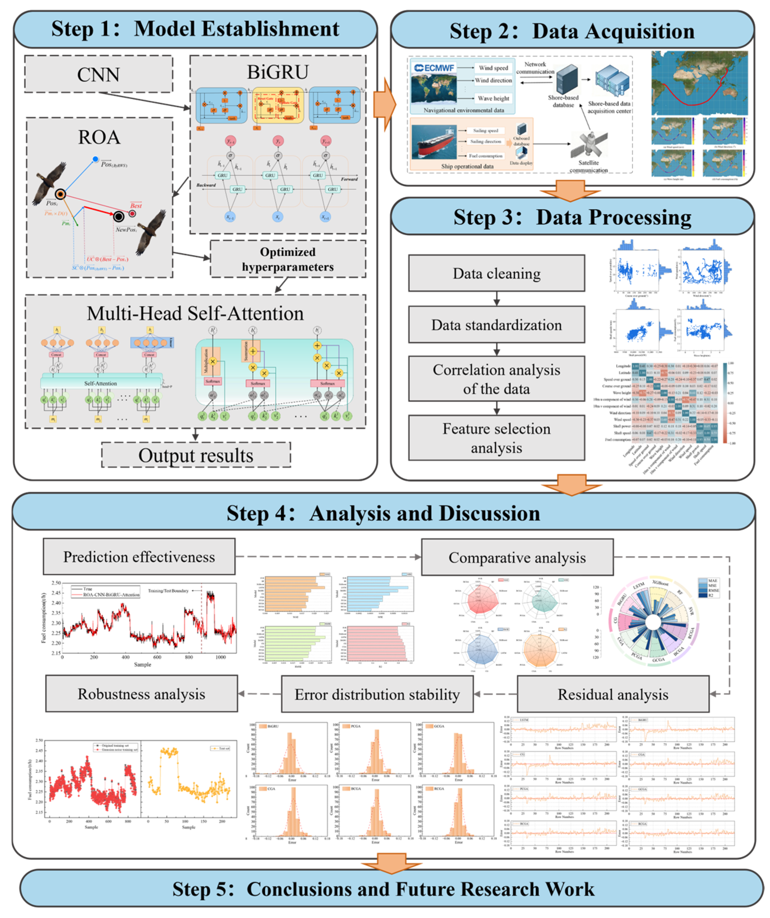
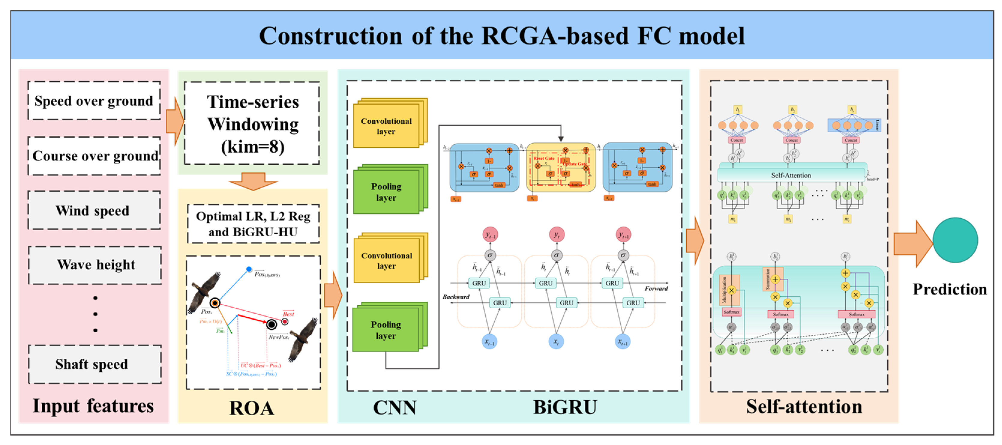
The construction of the RCGA model is depicted in Figure 1. The following are the specific steps: First, the real ship navigational environmental data and operational data collected by ECMWF and sensors are processed, and the input features of the RCGA model are selected using the Pearson correlation coefficient and cluster analysis. Second, the model extracts spatio-temporal features from multiple input data through the CNN-BiGRU-Attention hybrid network, introduces an attention mechanism to realize weighted fusion of key information, and enhances prediction capability of the model. Meanwhile, the ROA is employed to precisely optimize core hyperparameters including the learning rate (Lr), the number of hidden units, and the L₂ regularization (L₂) coefficient. Then, this proposed model is evaluated through case analysis and rigorous validation using actual navigation data.

2.1. CNN

The convolutional layer is the primary component of a CNN, performing scanning operations on input data using learnable convolutional kernels [42]. These kernels automatically extract local spatial features from the input, such as edges or textures, to form intermediate feature maps. Through downsampling, the pooling layer lowers the dimensionality of feature maps and computational complexity while preserving key feature information. The Fully Connected Layer (FCL) is responsible for mapping the extracted high-dimensional features to the final output space, enabling tasks like classification or regression.

2.2. BiGRU

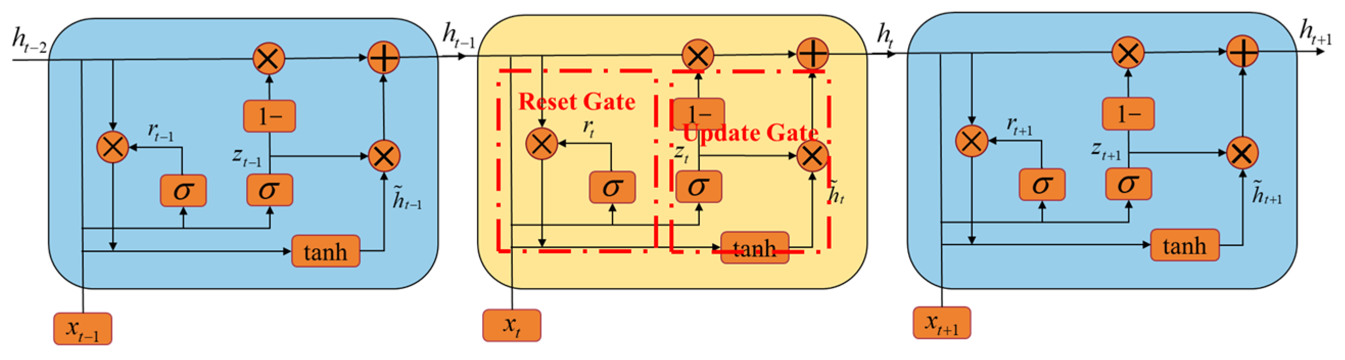
An update gate and a reset gate make up the main components of GRU. An update gate and a reset gate make up the main components of GRU. The architecture of GRU is illustrated in Figure 2.

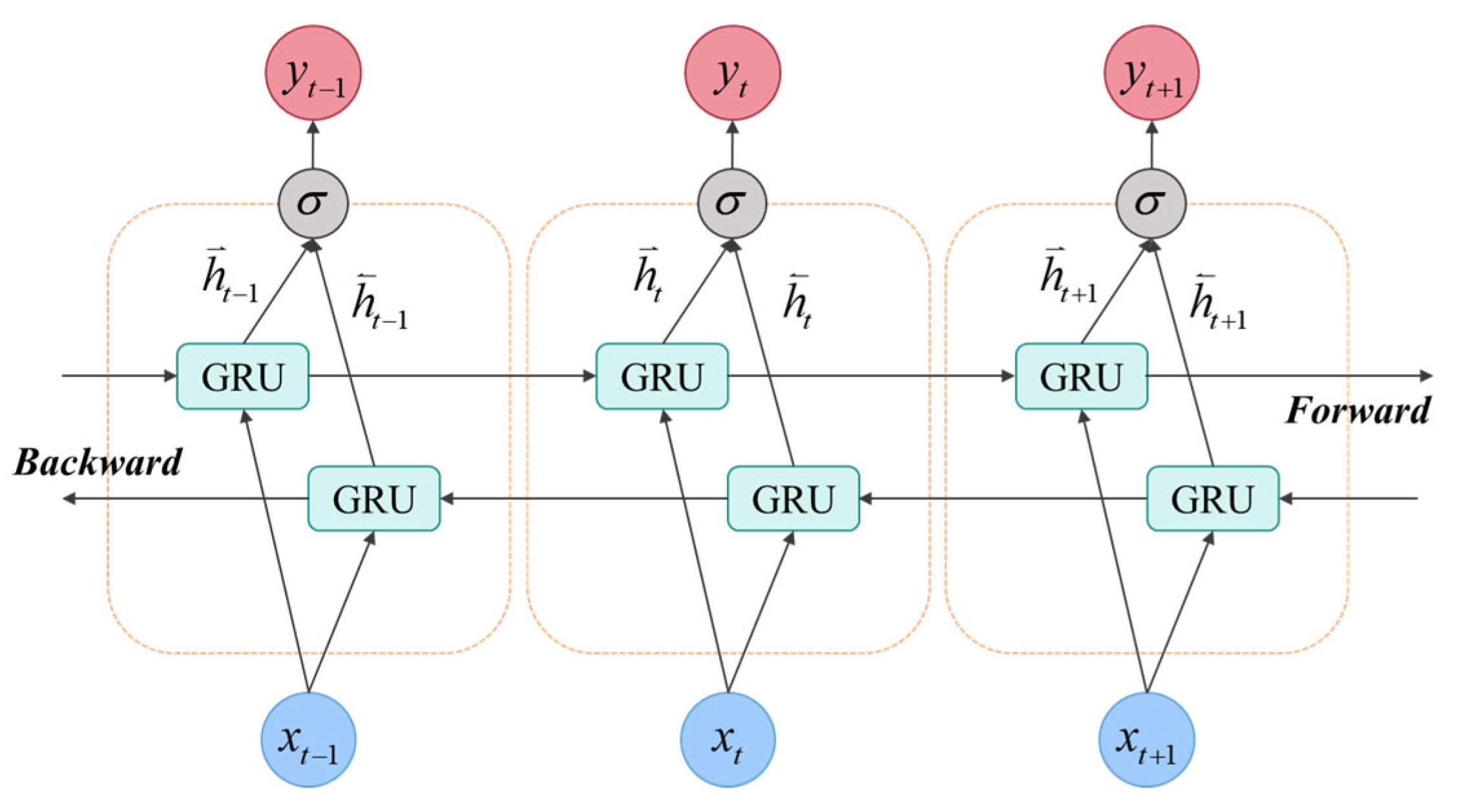
The BiGRU introduces a bidirectional mechanism on the basis of the GRU. By simultaneously training a forward GRU layer and a backward GRU layer, it captures both past and future temporal dependencies within the sequence [43]. The architecture of BiGRU is illustrated in Figure 3.

$$h_t=[{\stackrel{\rightharpoonup }{h}}_t;{\stackrel{\leftharpoonup }{h}}_t]$$

(1)

where ${\stackrel{\rightharpoonup }{h}}_t$ and ${\stackrel{\leftharpoonup }{h}}_t$ represent the information before and after time point $t$, respectively; $h_t$ is the final hidden state, and $[\cdot ;\cdot ]$ denotes the concatenation operation.

2.3. Multi-Head Self-Attention

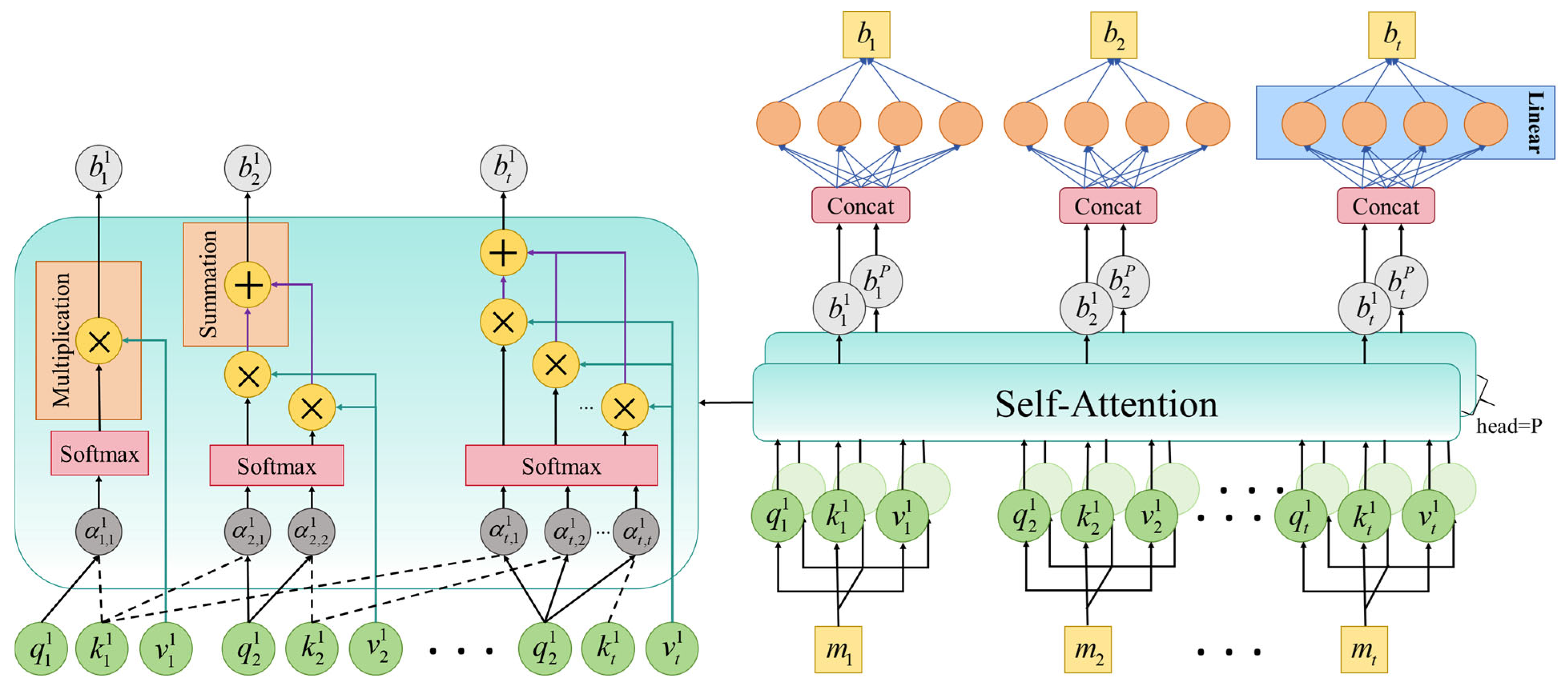
The principle of the multi-head self-attention [44] is illustrated in Figure 4. It can be seen that the dot-product attention value for the time-series data within head h can be expressed as:

$${\alpha }_{i,\delta }^h={\displaystyle \frac{q_i^h\times {(k_i^h)}^T}{\sqrt{d_k}}}$$

(2)

$$b_i^h={\displaystyle \sum _{\delta =1}^{i}Soft\max ({\alpha }_{i,\delta }^h)v_i^h}$$

(3)

$$b_i=Linear[Concat(b_i^1,b_i^2,L,b_i^P)]$$

(4)

where $\delta$ = 1, 2, …, $t$, and $d_k$ denotes a scaling factor designed to alleviate the vanishing gradient problem. The output from each individual attention head, $b^h$, is subsequently integrated via the Concat layer and the linear layer (linear) to yield the final output.

2.4. ROA

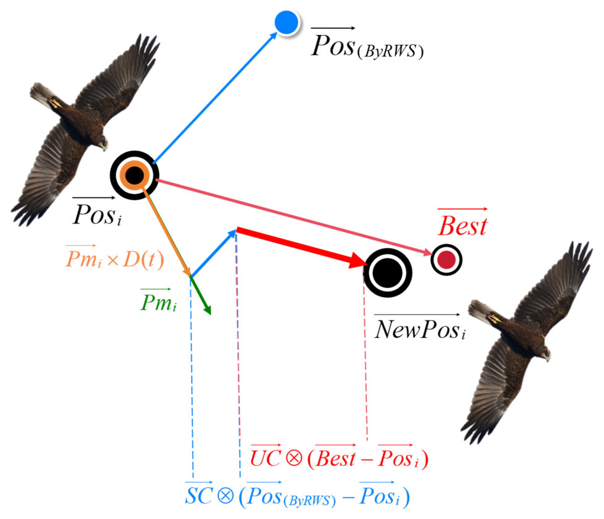
The ROA is characterized by computational efficiency, minimal hyperparameter tuning, and robust convergence properties [45]. The Red Kite’s new temporary position is determined by its current position and a displacement vector. The candidate position is updated only when the fitness value of the new position surpasses that of the current one. The movement mechanism of individual red kites in the ROA is illustrated in Figure 5.

$$\overrightarrow{NewPo{s}_i(t+1)}=\overrightarrow{Po{s}_i(t)}+\overrightarrow{P{m}_i(t+1)}$$

(5)

where $\overrightarrow{P{m}_i(t+1)}$ is the displacement vector.

3. Data Acquisition and Processing

3.1. Data Acquisition and Preprocessing

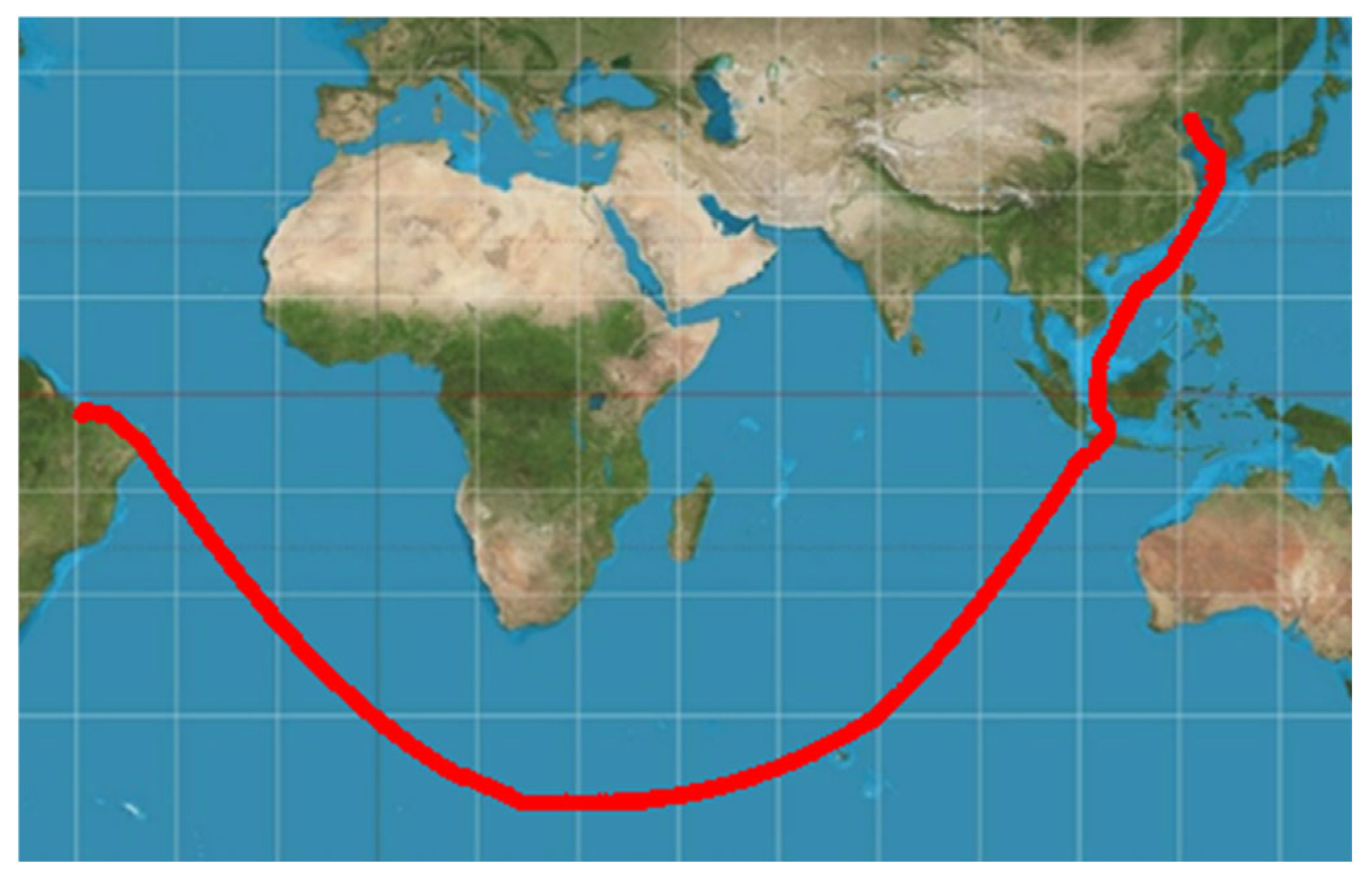
In this study, the voyage data of the M/V Yuzhonghai is selected as the experimental dataset. Specifically, the dataset includes the voyage information of the ship from St. Louis to Caofeidian. The Yuzhonghai is a bulk carrier, and its detailed parameters are presented in

Table 1. Main parameters of the ship.

Item	Parameter	Item	Parameter
Number of blades	5	Deadweight	297,959 t
Design speed	14.5 kn	Draft	21.4 m
Main engine speed	73 r/min	Length	327 m
Main engine power	19,000 kW	Depth	29 m
Diameter of propeller	9.7 m	Width	55 m

. The particular sailing route used in the experiment is illustrated in Figure 6.

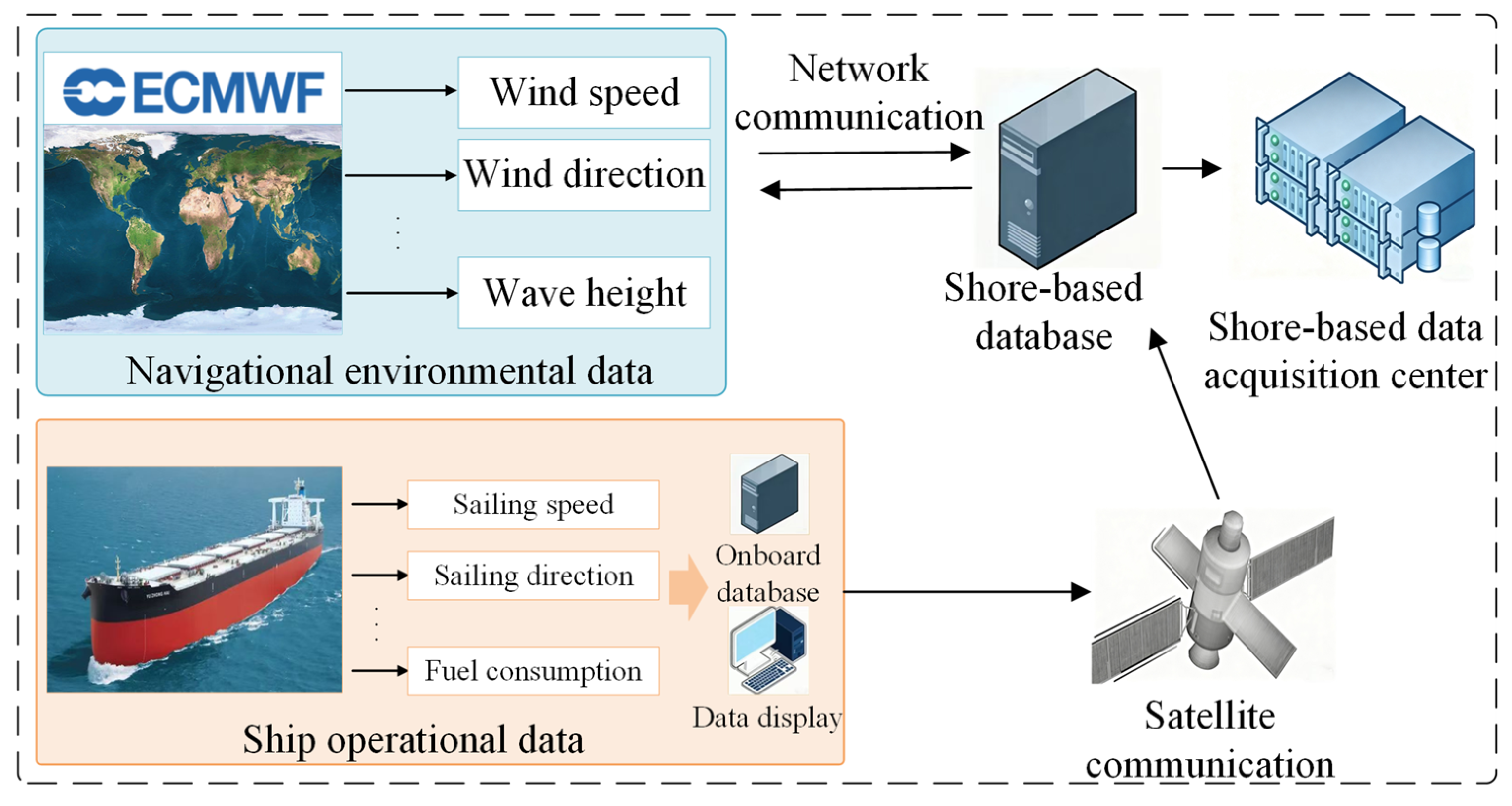
The actual operational data and navigational environmental data of the target ship can be acquired through the following systems, as illustrated in Figure 7. GPS, European Centre for Medium-Range Weather Forecasts (ECMWF), and various sensors collectively constitute the data acquisition system. Among them, corresponding equipment can be used to acquire ship operation status data, including shaft speed, sailing direction, sailing speed, and ship FC.

Data preprocessing is performed to account for the time scale discrepancy between the ship FC data and the navigational environmental data acquired from the meteorological center. First, the ship FC data, initially gathered at 10 min intervals beginning at 00:00 daily, are transformed into hourly time-series data. Then, based on GPS and ECMWF data, the frequency of meteorological and sea state data is adjusted using the cubic B-spline interpolation algorithm to ensure that the high-frequency shipboard measurement data and the low-frequency marine meteorological reanalysis data are temporally aligned. Compared with traditional methods, cubic B-spline interpolation exhibits superior performance due to its good accuracy and modest computational complexity [46], thereby enabling more accurate results. The normalized cubic B-spline interpolation can be elegantly defined as weighted summation.

$$s(d)={\displaystyle \sum _{k=1}^{4}c(k)B^3(k-d)}$$

(6)

where $c(k)$ is the B-spline coefficients to be determined from input data, which are four equally spaced data points along one dimension. $d$ is the sub-coordinate between $k$ = 2 and $k$ = 3, which means $d$ $\in$ [0, 1]. $B^3(x)$ is the function of cubic B-spline. $s(d)$ denotes the output value obtained after cubic B-spline interpolation.

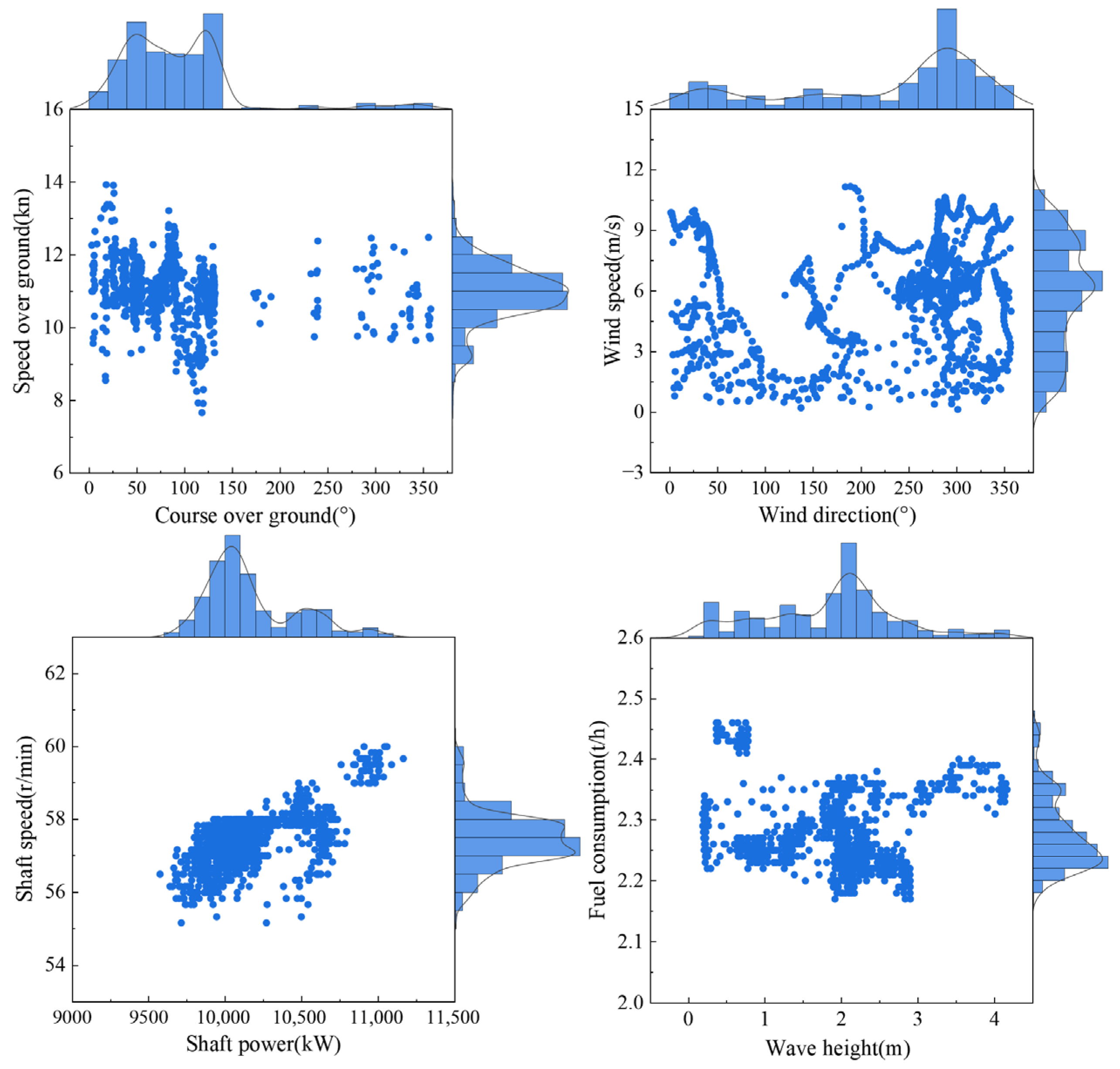
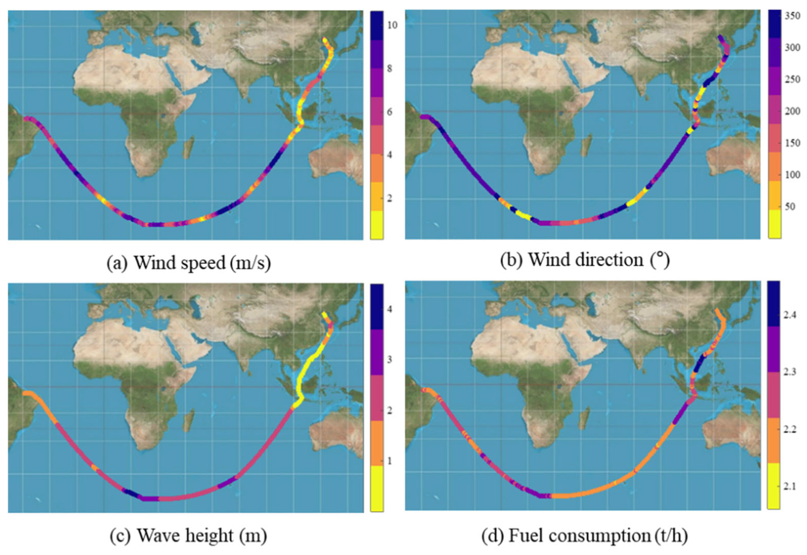
In addition, strict data cleaning is performed to eliminate outliers and sensor noise. The distributions of environmental characteristics and FC are shown in Figure 8. It can be observed that environmental characteristics such as wave height, wind direction, and wind speed exhibit distinct non-stationary time series characteristics during ship operation, which correlate strongly with the fluctuation of FC. It is evident that environmental factors have a significant impact on ship FC.

3.2. Correlation Analysis

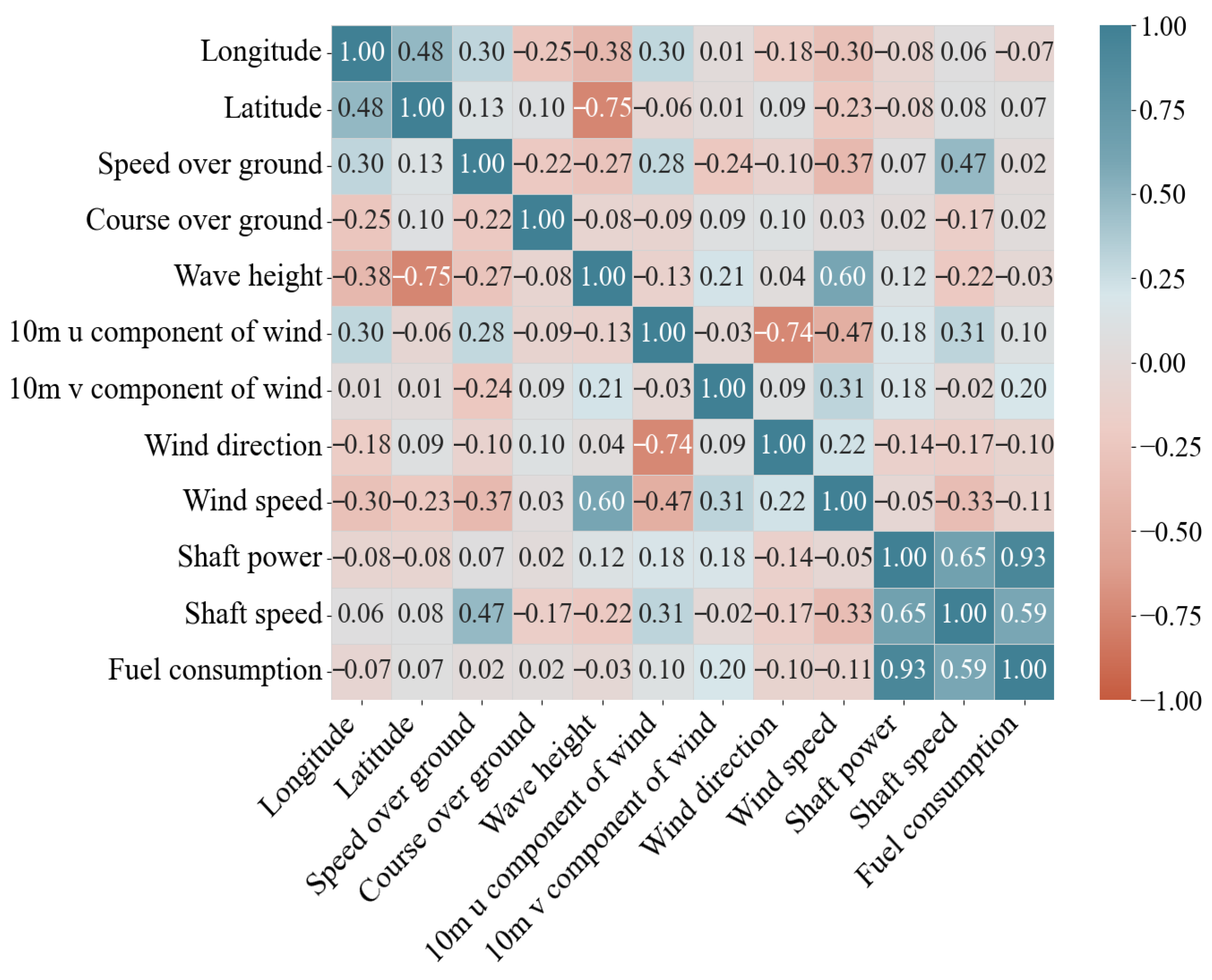
The ship FC is the result of the coupled effects of multiple factors. The acquired data are presented in

Table 2. The acquired data of the target ship.

Type	Feature	Unit
Navigational environmental data	Longitude	°
	Latitude	°
	Wave height	m
	Wind speed	m/s
	Wind direction	°
	10 m u component of wind	m/s
	10 m v component of wind	m/s
Ship operational data	Speed over ground	kn
	Course over ground	°
	Shaft speed	r/min
	Shaft power	kW
	Fuel consumption	t/h

. In addition, the Pearson correlation coefficient method is employed to analyze the linear correlation between each feature variable and the FC. The correlation among the feature variables is illustrated in Figure 9. The correlation coefficient between shaft power and FC reaches 0.93, while that between shaft speed and FC is 0.59. This observation is highly consistent with the physical mechanism that the main engine output power and rotation speed are the most direct driving factors for ship propulsion FC. The correlation of wind speed and sailing speed with FC is relatively lower; however, their influence mechanisms are more complex, often involving nonlinear mapping relationships.

3.3. Feature Selection

The distribution of relevant operational data for the target sailing route is presented in Figure 10. The wind speed is found to be mostly dispersed between 0 and 12 m/s, suggesting that the proposed model is trained in windy settings, increasing its capacity to adapt to intricate marine environments. The wave height is concentrated between 2 and 3 m, which has a significant impact on FC. Meanwhile, the ship FC is mostly concentrated at 2.2–2.4 t/h. The speed over ground is mostly between 10 and 14 knots, which is primarily influenced by the complex navigation environment.

Concurrently, to accurately capture the instantaneous dynamic variations in ship FC under different maneuvering and heading conditions, this study employs the DBSCAN clustering method to analyze historical voyage data. The non-linear impact of maneuvering and heading adjustments on FC is significant. Given that maneuvering involves complex dynamic and kinematic processes, its prediction is generally categorized as an ultra-short-term forecasting task, which imposes stringent requirements on both real-time performance and prediction accuracy [47].

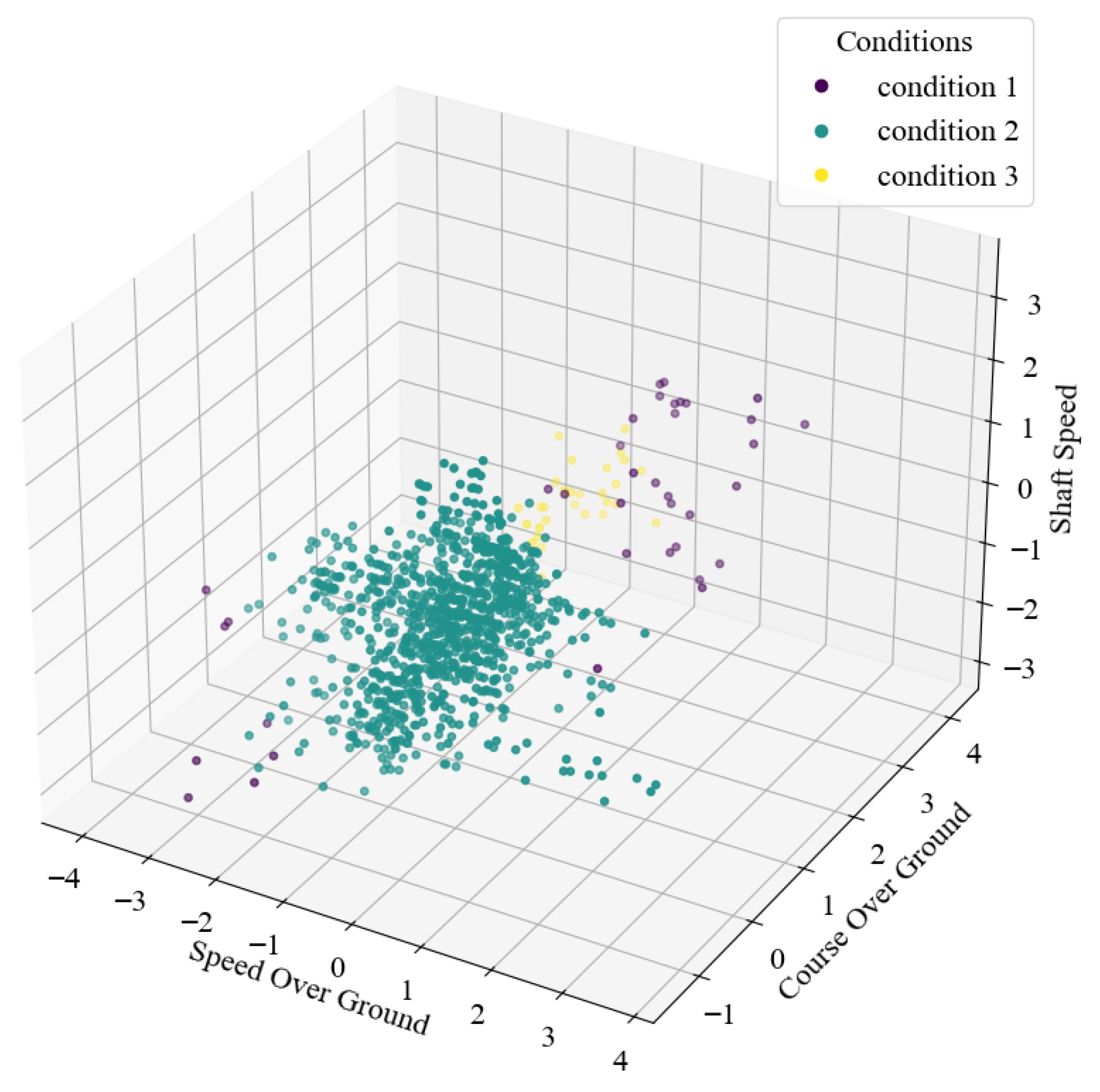
The cluster table of features is presented in

Table 3. The cluster table of features.

Features	Condition 1	Condition 2	Condition 3
Count	38	1033	29
Speed over ground mean	10.82	10.97	10.12
Speed over ground standard deviation	1.38	0.78	0.33
Course over ground mean	245.58	81.06	318.07
Course over ground standard deviation	104.72	37.40	36.50
Shaft speed mean	57.04	57.45	56.55
Shaft speed standard deviation	0.91	0.73	0.41
Shaft power mean	10,141.54	10,173.42	10,041.95
Shaft power standard deviation	201.95	303.27	99.38

. It can be seen that the speed over ground, course over ground, shaft speed, and shaft power are selected as the input feature vectors for the DBSCAN algorithm. Among these, ship resistance exhibits a cubic relationship with speed over ground, such that a slight increase in speed over ground leads to a nonlinear surge in ship FC; variations in course over ground alter the relative angles of wind, waves, and currents encountered by the vessel, thereby influencing the added resistance; shaft speed is positively correlated with propeller thrust, and the main engine FC rate exhibits a nonlinear positive correlation with shaft speed; shaft power directly corresponds to the FC of the main engine and can reflect the energy output efficiency of the ship under current operating conditions. By applying the DBSCAN clustering method, discrete transient operational data are identified and condensed into structured ship operating condition labels, which serve as key input features. The voyage data are clustered into three distinct operating conditions. Condition 1 characterizes the transient maneuvering state, which includes frequent speed adjustments and course alterations. The high standard deviations in speed over ground and course over ground reflect intense ship dynamics, necessitating higher model sensitivity to capture instantaneous energy fluctuations. Condition 2 corresponds to the steady-state cruising condition, representing the majority of the dataset. It is characterized by the highest mean speed over ground and shaft power combined with low standard deviations, indicating stable, long-duration voyages at cruising speed. This condition serves as the primary operational baseline for FC. Condition 3 represents low-speed restricted navigation. All parameters and their standard deviations are at their minimum levels, reflecting a state where the ship maintains a consistent but reduced speed, typically encountered in high-traffic or environmentally sensitive waterways. The clustering results are illustrated in Figure 11.

Based on the cluster analysis results, the remaining seven variables are chosen as the input features for the RCGA model. These features include: speed over ground, course over ground, shaft power, wave height, shaft speed, wind direction, and wind speed. Specifically, the wind speed is synthesized from the original data vectors.

4. Model Performance and Case Study

This chapter comprehensively evaluates the performance of the proposed RCGA-based model for ship FC prediction using quantitative metrics and visualization results. The framework of the RCGA model is shown in Figure 12.

4.1. Parameter Settings and Performance Metrics

In order to ensure the dependability and impartiality of the model evaluation, the dataset division and the hyperparameter configuration for model training are strictly standardized. The cleaned raw voyage data samples are separated into an 8:2 training set and a testing set in exact chronological order. To optimize model learning efficiency and monitor generalization ability during training, the last 20% of the training set data is further designated as the validation set. Furthermore, a sliding time window strategy with a time window size of 8 is adopted in this study, where feature data from eight consecutive time steps are flattened to serve as a single sample input to the model, ensuring the full capture of temporal characteristics. The specific configuration is shown in

Table 4. RCGA model hyperparameter configuration.

Parameters	Values	Value Range
Time Window	8	-
Optimizer	Adam	-
Loss Function	Mean Squared Error	-
Lr	Decreases by 10% every 25 times	[0.0001, 0.001]
Hidden Units	-	[8, 64]
L2	-	[0.0001, 0.001]
Batch_size	16	-
Epoch	150	-
ROA Population	5	-
ROA Max Iterations	10	-

.

In addition, the identical parameters for other comparative experimental models are maintained consistent with this model, and the remaining differing parameters are set to optimal values. The following four standard metrics are adopted to quantitatively evaluate the model prediction performance: Mean Absolute Error (MAE), Mean Squared Error (MSE), Root Mean Squared Error (RMSE) and coefficient of determination (R²).

4.2. Model Prediction Effectiveness

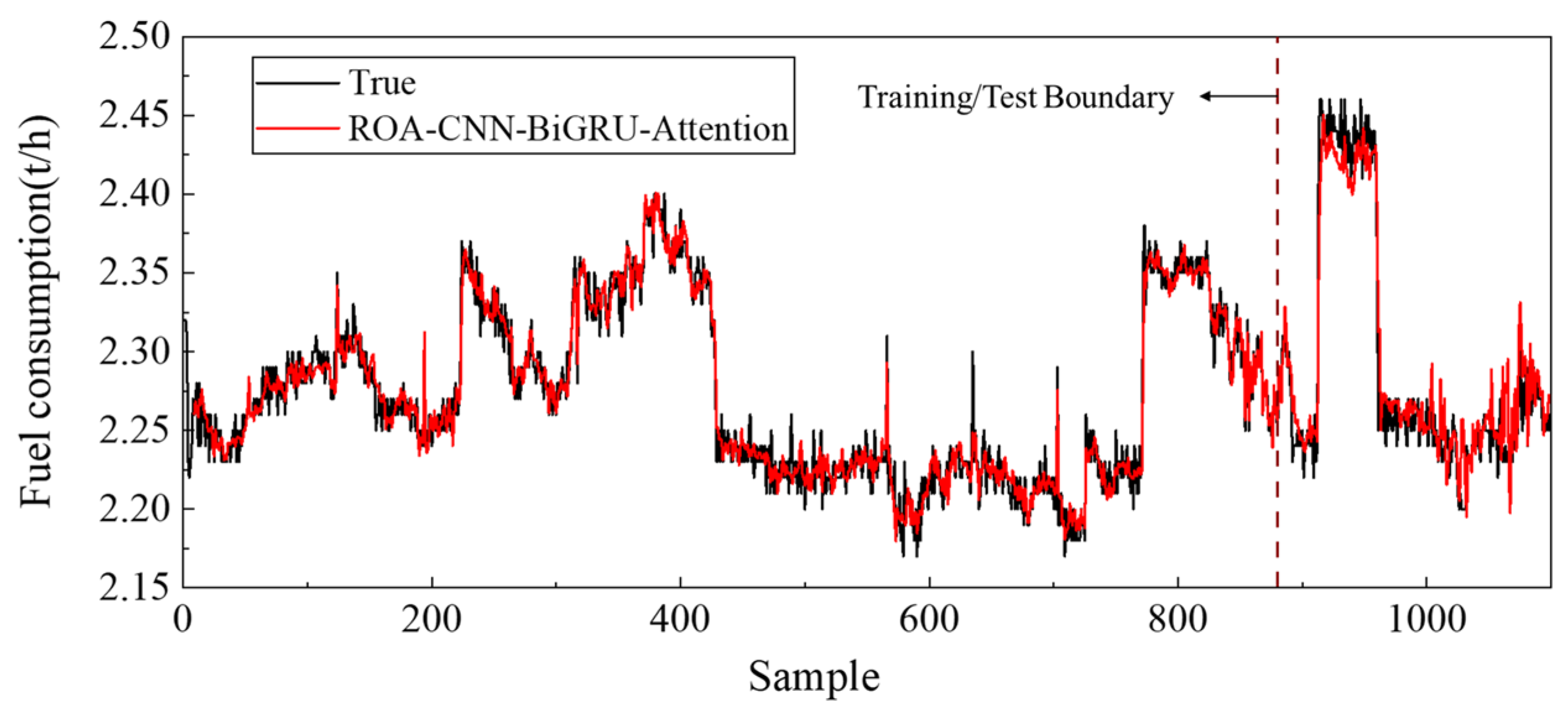
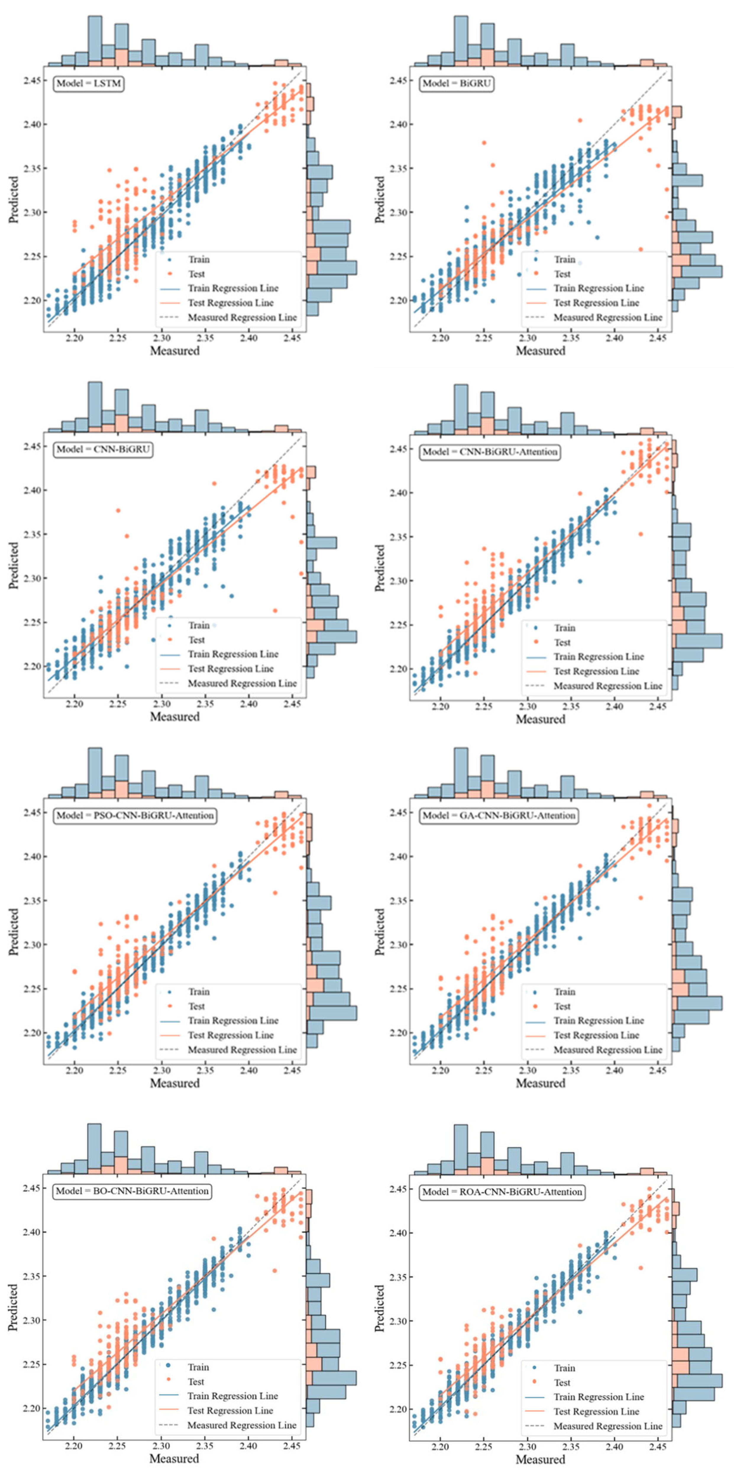
Following data processing and feature selection, a total of 1100 valid data samples are obtained for the analyzed voyage. The RCGA model is established using MATLAB R2024a, and all experiments are conducted on a 64-bit Windows 11 operating system. The proposed model is experimentally validated, and the prediction results obtained by the RCGA are illustrated in Figure 13. Additionally, we have compared the prediction performance of different models. The prediction results for different models are illustrated in Figure 14. It is evident that the RCGA model exhibits good predictive performance, and its prediction effect is superior to other models such as SVR, RF, and XGBoost, thereby verifying the prediction accuracy and strong generalization capability of the RCGA model.

4.3. Comparative Analysis

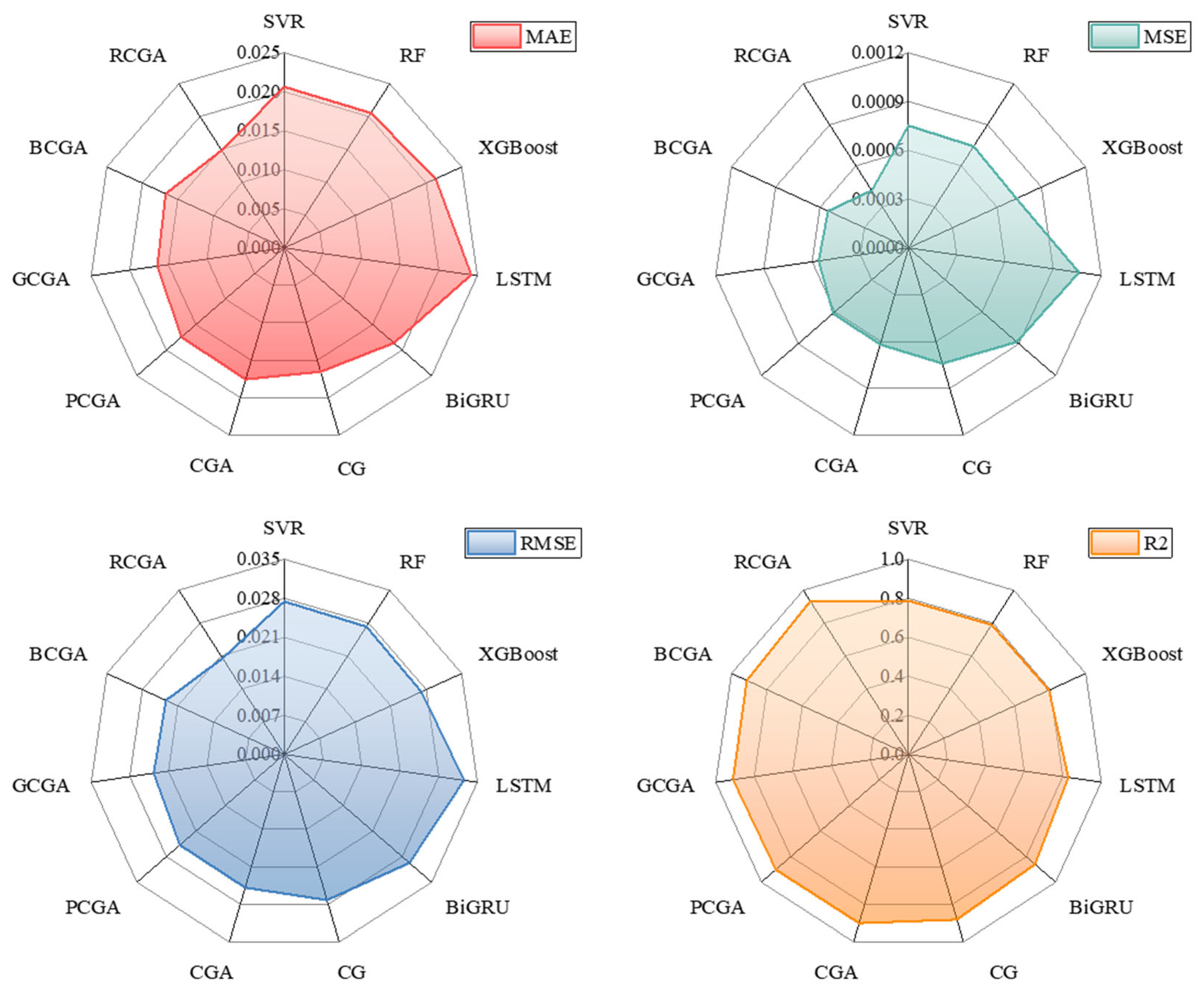
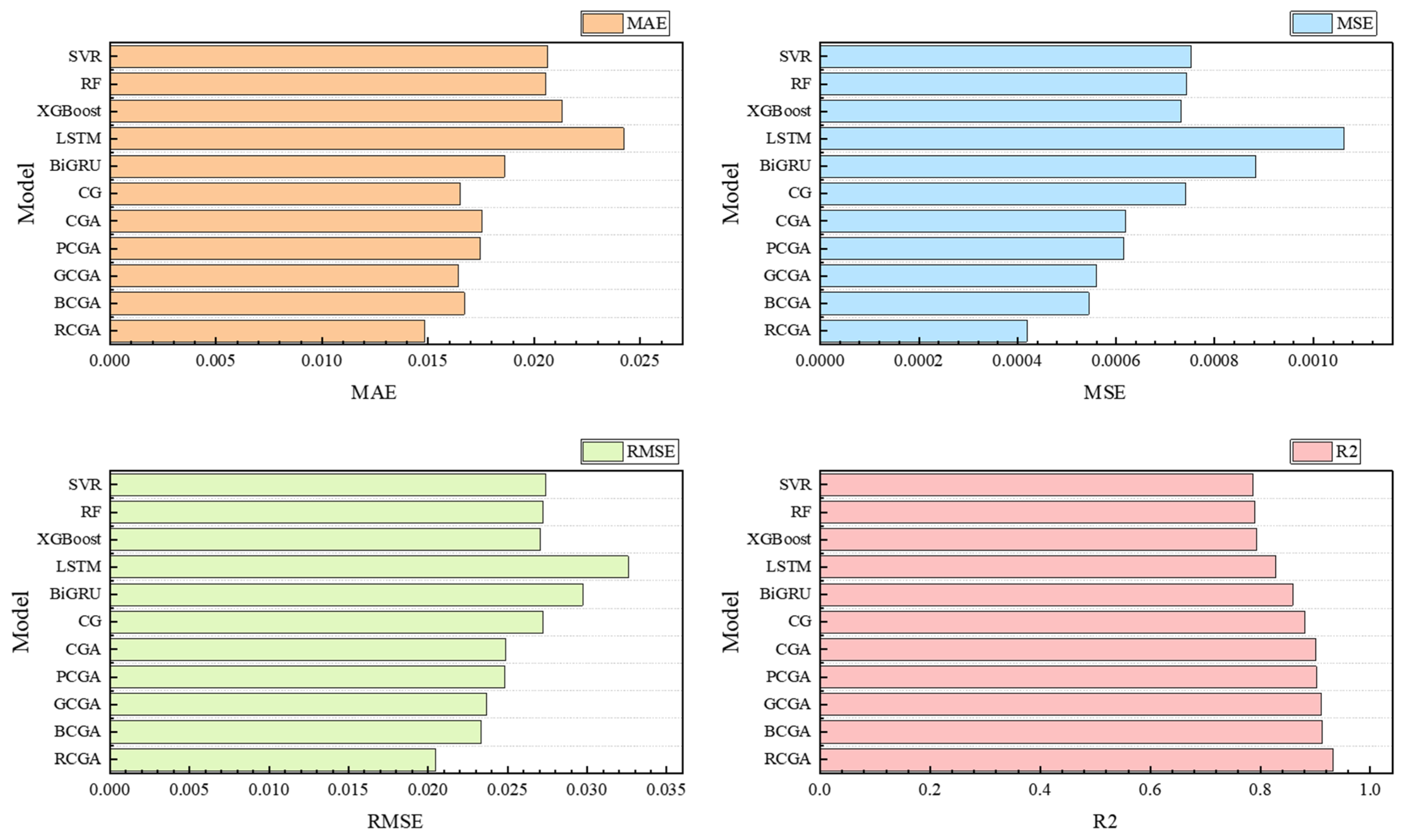
By presenting a number of benchmark models and optimized variations, this part offers a thorough quantitative assessment of the RCGA model.

Table 5. The prediction accuracy of different models.

Models	MAE	MSE	RMSE	R2
SVR	0.0206	0.0008	0.0274	0.7874
RF	0.0205	0.0007	0.0272	0.7901
XGBoost	0.0213	0.0007	0.0270	0.7932
LSTM	0.0242	0.0011	0.0326	0.8289
BiGRU	0.0186	0.0009	0.0297	0.8589
CNN-BiGRU (CG)	0.0165	0.0007	0.0272	0.8817
CNN-BiGRU-Attention (CGA)	0.0176	0.0006	0.0249	0.9010
PSO-CNN-BiGRU-Attention (PCGA)	0.0174	0.0006	0.0248	0.9018
GA-CNN-BiGRU-Attention (GCGA)	0.0164	0.0006	0.0237	0.9106
BO-CNN-BiGRU-Attention (BCGA)	0.0167	0.0005	0.0233	0.9130
ROA-CNN-BiGRU-Attention (RCGA)	0.0149	0.0004	0.0205	0.9330

displays the prediction accuracy of several models, and the comparison of prediction performance is shown in Figure 15 and Figure 16. It is evident that the RCGA model performs best in FC prediction, achieving a coefficient of determination R² as high as 0.9330, while its MAE, MSE, and RMSE values are the lowest, displaying its noteworthy superiority in terms of prediction accuracy and showcasing its substantial edge in this area.

In particular, the RCGA model outperforms SVR, RF, XGBoost, LSTM, BiGRU, CNN-BiGRU (CG), CNN-BiGRU-Attention (CGA), PSO-CNN-BiGRU-Attention (PCGA), GA-CNN-BiGRU-Attention (GCGA), and BO-CNN-BiGRU-Attention (BCGA) models on multiple indicators: R² is increased by 8.50%, 18.09%, 17.63%, 12.57%, 8.63%, 5.82%, 3.55%, 3.46%, 2.47%, 2.19%, respectively; MAE is decreased by 28.00%, 27.70%, 30.33%, 38.68%, 20.14%, 10.15%, 15.38%, 14.83%, 9.66%, 11.12%, respectively; MSE is decreased by 44.25%, 43.50%, 60.52%, 52.53%, 43.40%, 32.36%, 31.79%, 25.12%, 23.02%, respectively; RMSE is decreased by 25.31%, 24.83%, 24.28%, 37.16%, 31.10%, 24.77%, 17.75%, 17.41%, 13.47%, 12.26%.

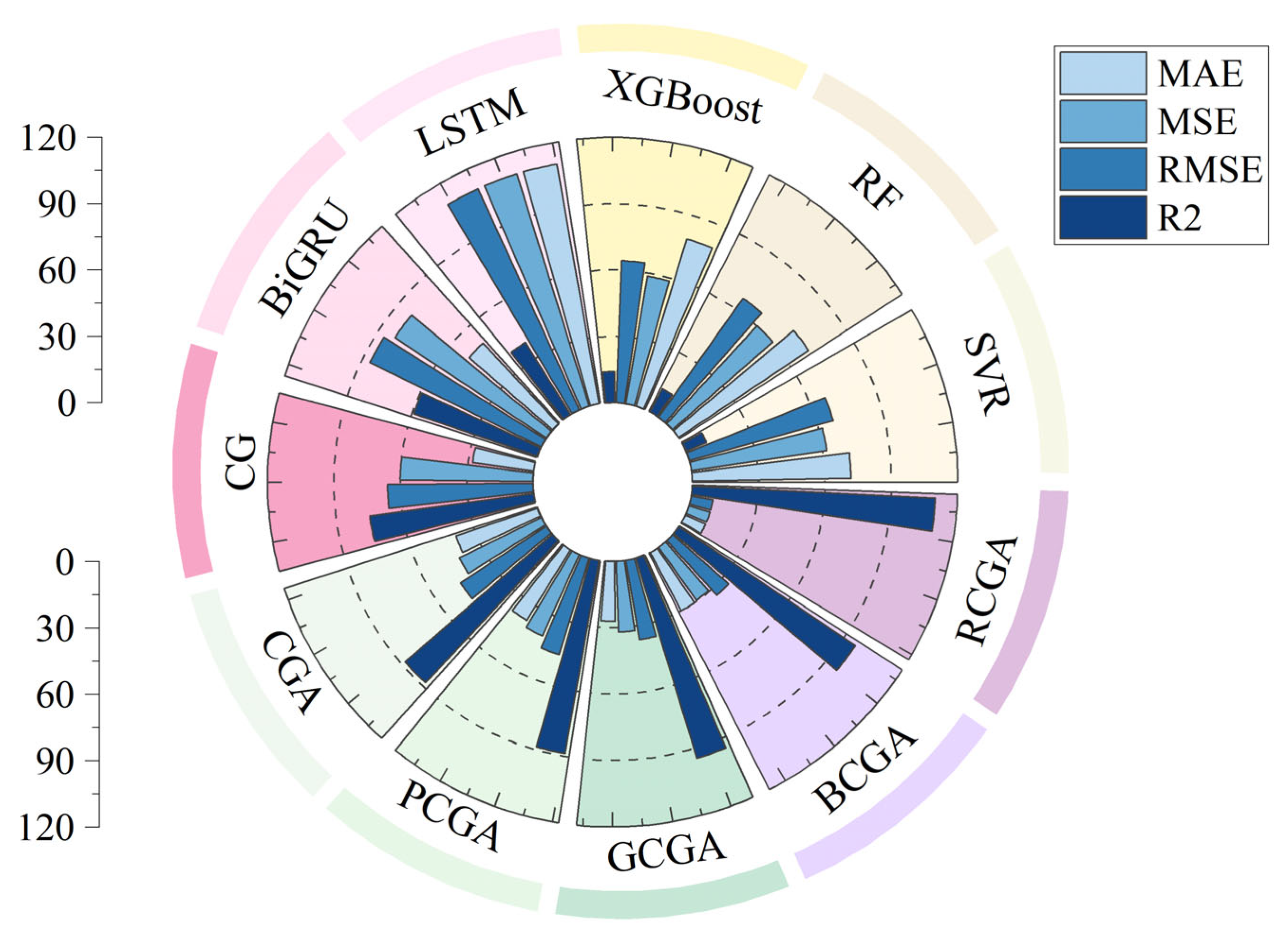
It is noteworthy that due to the significant disparity in the orders of magnitude of the four key metrics, the data indicators presented in Figure 17 are subjected to a transformation process to facilitate simultaneous visualization. All original experimental results are normalized using the Min-Max normalization method according to the following formula:

$$x_{normalized}={\displaystyle \frac{x-x_{\min }}{x_{\max }-x_{\min }}}$$

(7)

where $x_{normalized}$ is the normalized data value; $x$ is the original data value; $x_{\min }$ is the minimum value in the original dataset; and $x_{\max }$ is the maximum value in the original dataset.

Subsequently, a linear transformation was applied to the data using the following formula:

$$f(x)=10x_{normalized}+10$$

(8)

The processed data are presented in

Table 6. Normalized and transformed performance metrics.

Model	MAE	MSE	RMSE	R2
SVR	71.64	61.77	67.32	10.00
RF	70.74	60.21	65.86	11.88
XGBoost	79.03	58.50	64.22	13.97
LSTM	110.00	110.00	110.00	38.48
BiGRU	49.97	82.19	86.35	59.12
CG	27.91	60.00	65.67	74.75
CGA	38.82	41.20	46.51	88.01
PCGA	37.61	40.40	45.66	88.57
GCGA	26.96	31.88	36.32	94.58
BCGA	29.84	29.50	33.63	96.25
RCGA	10.00	10.00	10.00	110.00

. Experimental results indicate that the MAE, MSE, and RMSE values of the RCGA model reached the minimum critical value of 10, demonstrating that these three metrics for this model are the lowest among all comparative experiments. Conversely, the R² value reached the maximum critical value of 110, indicating that this model achieves the best performance.

5. Model Performance Analysis and Discussions

5.1. Residual Analysis

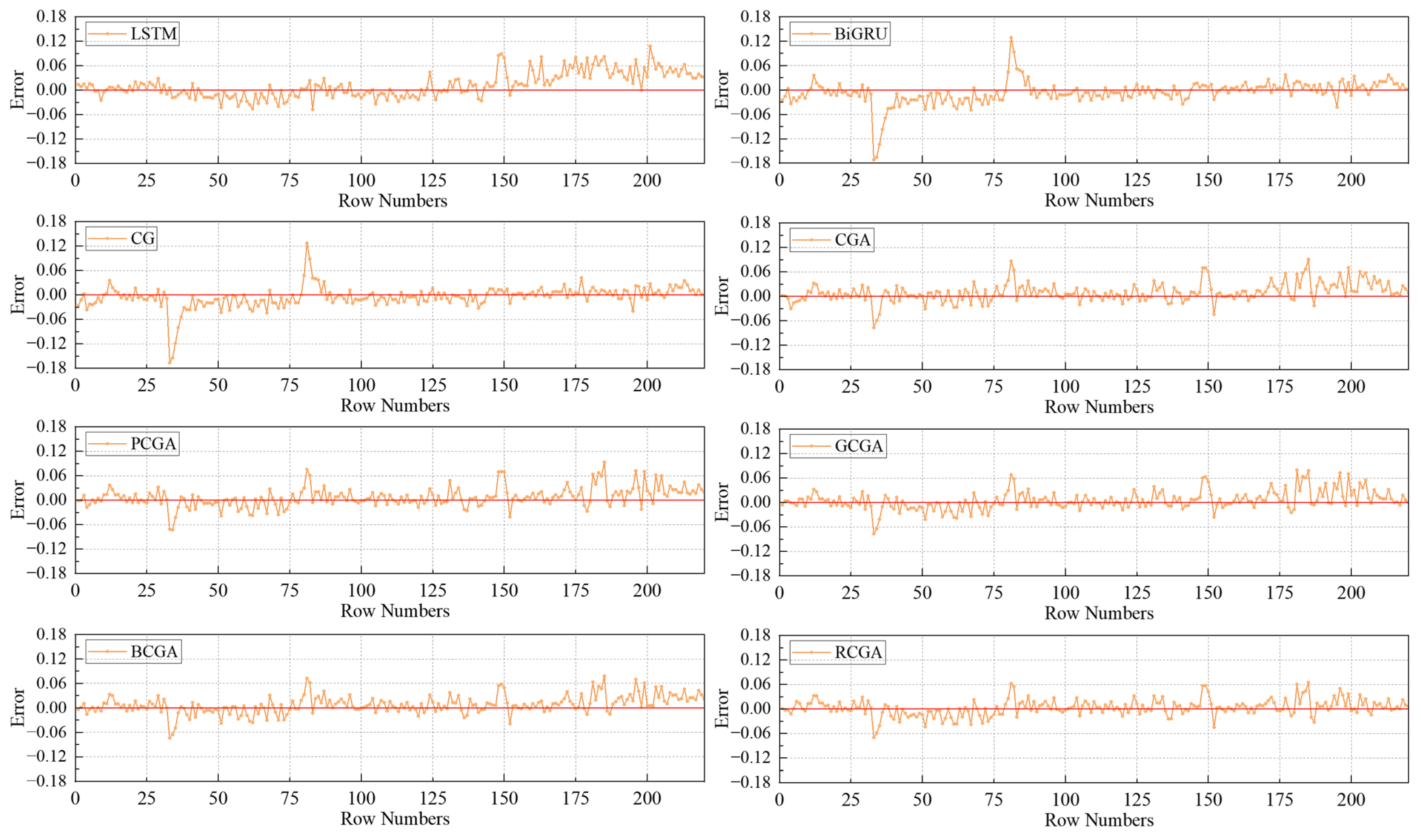
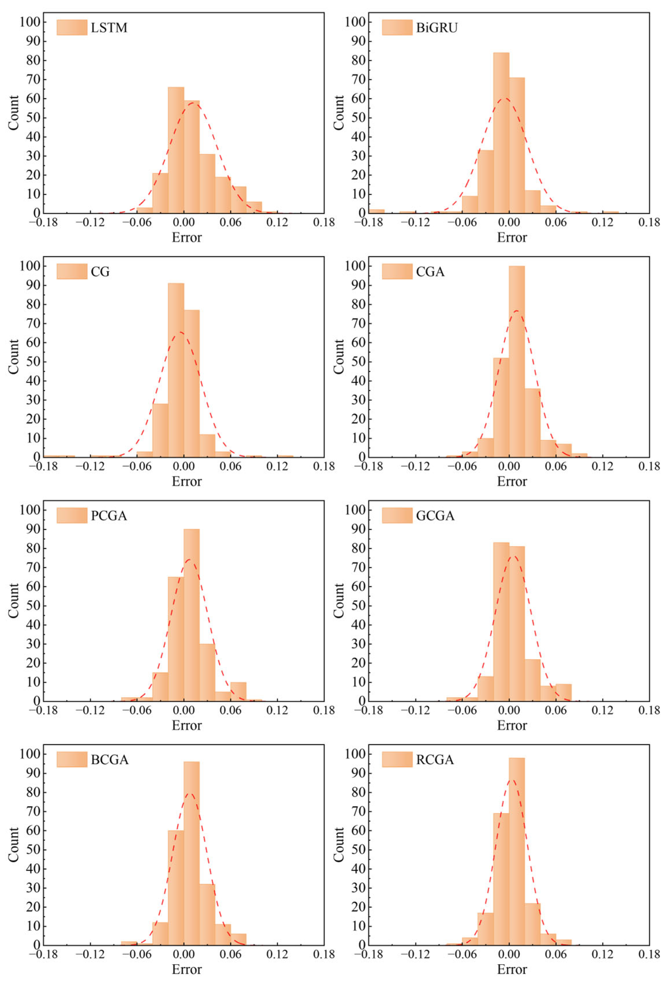
The residual line graph and relative error histogram of each model are shown in Figure 18 and Figure 19. The dashed red lines represent the Gaussian distribution fitting curve of the error for each model in Figure 19. It is evident that the RCGA model performs accurately and steadily because the relative error distribution is concentrated close to zero and follows a normal distribution. As a result, the RCGA model outperforms the others in terms of increasing prediction stability and accuracy.

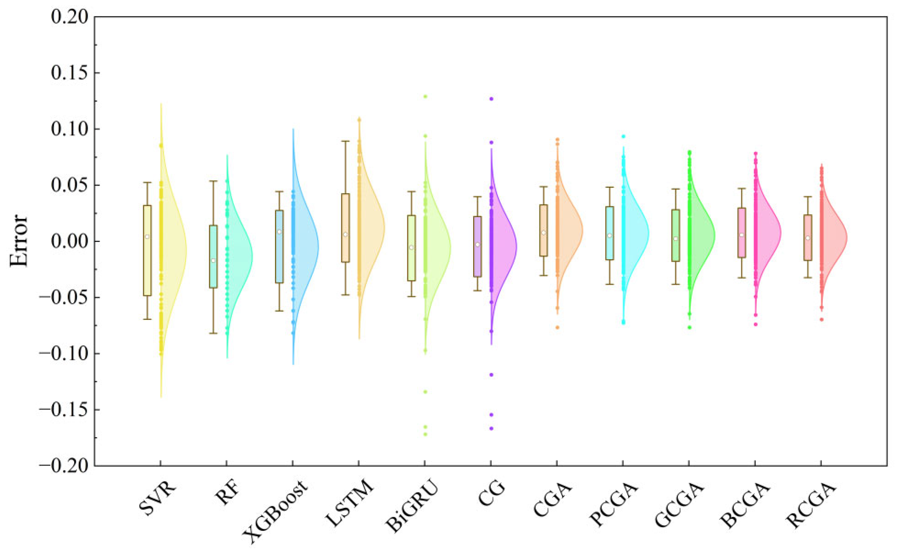
By comparing the probability density distributions of the residuals of different prediction models, the predictive stability of the models can be evaluated. The distribution of residuals is shown in Figure 20. It is evident that compared with the traditional benchmark models such as SVR, RF, XGBoost, LSTM, BiGRU, and CG, the models optimized by algorithms such as PCGA, GCGA, and BCGA exhibit significantly narrower violin widths and more tightly concentrated distributions near the error centerline (Error = 0). Moreover, the proposed RCGA model shows shorter tails and fewer outliers, indicating a more compact and convergent error distribution.

5.2. Robustness Analysis

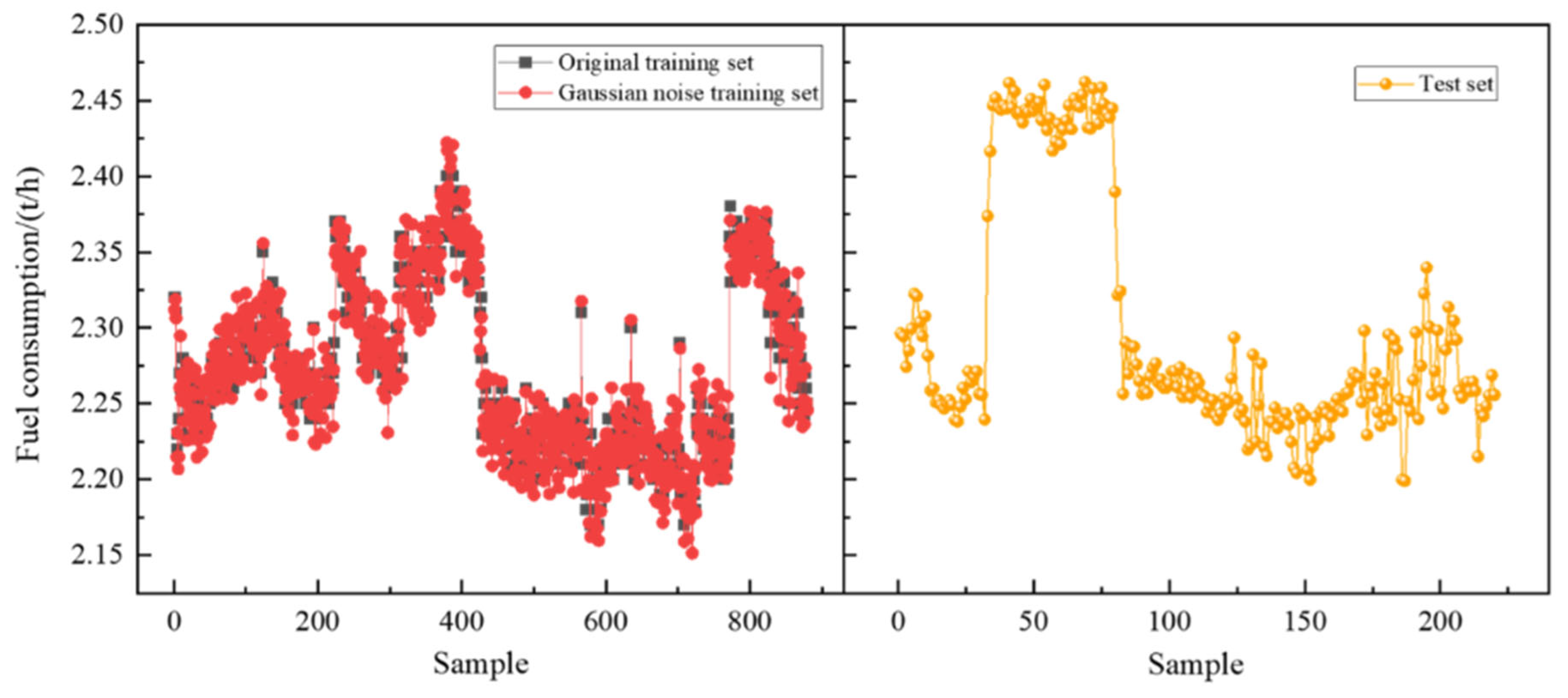
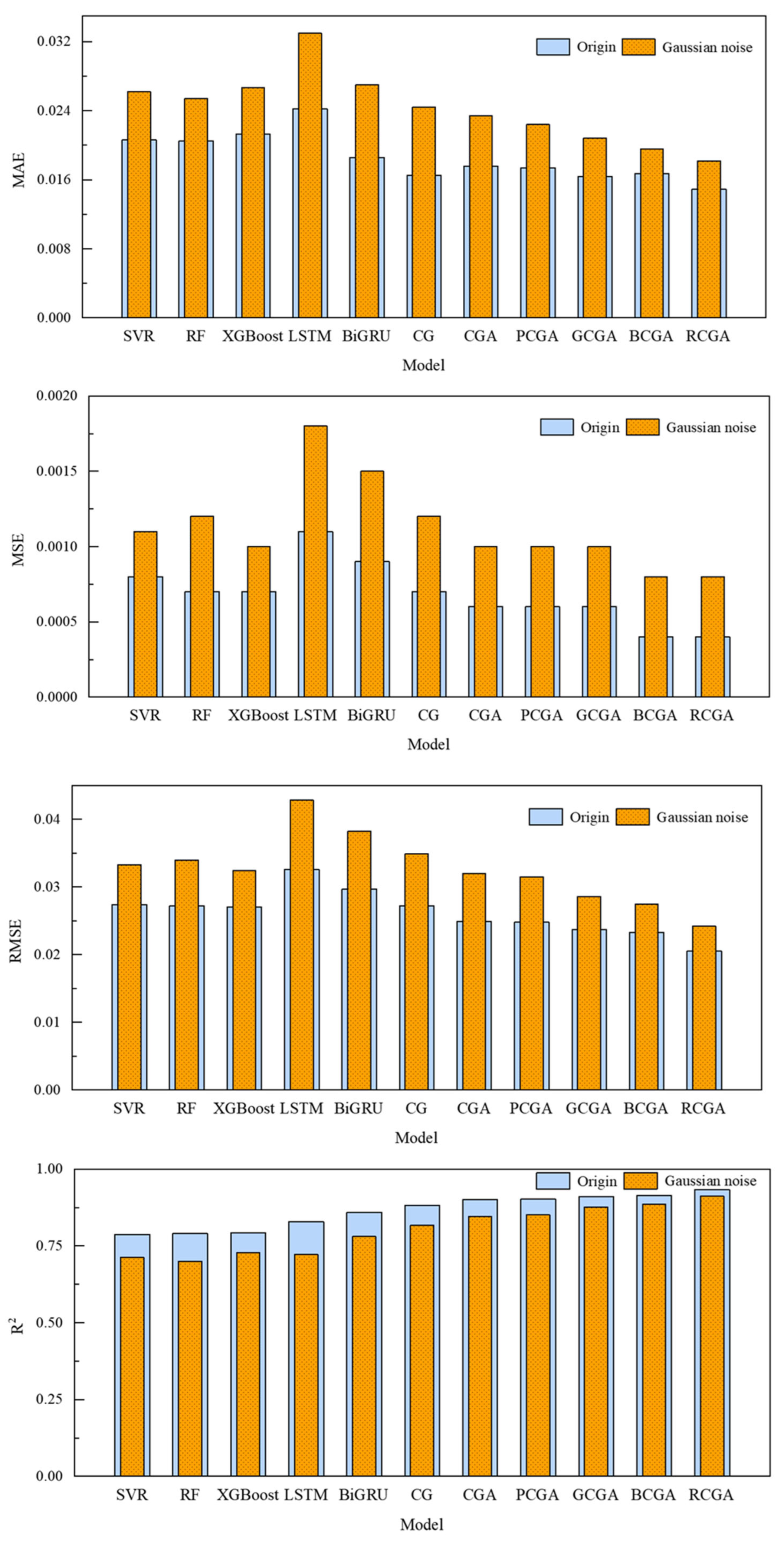
For the purpose of further analyzing the adaptability of the RCGA model under non-standard scenarios such as sensor equipment failure and noisy environments, a robustness analysis of the model is conducted in this section. Since the operational status and measurement accuracy of sensors are susceptible to interference from factors such as temperature, humidity, and electromagnetic effects—which can lead to data noise—the Gaussian method is employed in this study to process the FC data in the training set. Gaussian noise with a standard deviation of 0.0120 (0.2 times the standard deviation of the original FC data) is added to the original FC data, while the test set data remains unchanged [48].

The comparison between Gaussian noise data and the original data is shown in Figure 21. It can be observed that the Gaussian noise-processed data differ significantly from the original data. The noise-affected data exhibit varying degrees of deviation, indicating a higher level of interference. The performance of different models is shown in Figure 22. The presence of noise substantially affects data accuracy, causing a notable degradation in the prediction performance of all models. Here, N stands for the data noise scenario and O for the original data situation. The performance of different models is summarized in

Table 7. The performance comparison list of different models.

Model	Data Set	MAE	MSE	RMSE	R2
SVR	Origin	0.0206	0.0008	0.0274	0.7874
	Gaussian noise	0.0262	0.0011	0.0333	0.7121
RF	Origin	0.0205	0.0007	0.0272	0.7901
	Gaussian noise	0.0254	0.0012	0.0340	0.7003
XGBoost	Origin	0.0213	0.0007	0.0270	0.7932
	Gaussian noise	0.0267	0.0010	0.0324	0.7276
LSTM	Origin	0.0242	0.0011	0.0326	0.8289
	Gaussian noise	0.0330	0.0018	0.0428	0.7219
BiGRU	Origin	0.0186	0.0009	0.0297	0.8589
	Gaussian noise	0.0270	0.0015	0.0382	0.7804
CG	Origin	0.0165	0.0007	0.0272	0.8817
	Gaussian noise	0.0244	0.0012	0.0349	0.8175
CGA	Origin	0.0176	0.0006	0.0249	0.9010
	Gaussian noise	0.0234	0.0010	0.0320	0.8459
PCGA	Origin	0.0174	0.0006	0.0248	0.9018
	Gaussian noise	0.0224	0.0010	0.0315	0.8512
GCGA	Origin	0.0164	0.0006	0.0237	0.9106
	Gaussian noise	0.0208	0.0008	0.0286	0.8769
BCGA	Origin	0.0167	0.0005	0.0233	0.9130
	Gaussian noise	0.0196	0.0008	0.0275	0.8860
RCGA	Origin	0.0149	0.0004	0.0205	0.9330
	Gaussian noise	0.0182	0.0006	0.0242	0.9115

. However, the prediction effect of the RCGA model with added Gaussian noise is better than that of other models. Specifically, the R² of the RCGA model is increased by 28.00%, 30.16%, 25.27%, 26.26%, 16.80%, 11.50%, 7.76%, 7.08%, 3.95% and 2.88%, compared with the SVR, RF, XGBoost, LSTM, BiGRU, CG, CGA, PCGA, GCGA, and BCGA models, respectively. In addition, the RMSE is decreased by 27.33%, 28.82%, 25.31%, 43.46%, 36.65%, 30.66%, 24.38%, 23.17%, 15.38% and 12.00%, respectively; the MSE is decreased by 45.45%, 50.00%, 40.00%, 66.67%, 60.00%, 50.00%, 40.00%, 40.00%, 25.00% and 25.00%, respectively; the MAE is decreased by 30.53%, 28.35%, 31.84%, 44.85%, 32.59%, 25.41%, 22.22%, 18.75%, 12.50% and 7.14%. Above all, the proposed RCGA model demonstrates strong robustness even on the data with noise.

5.3. Equipment Failure Scenario Analysis

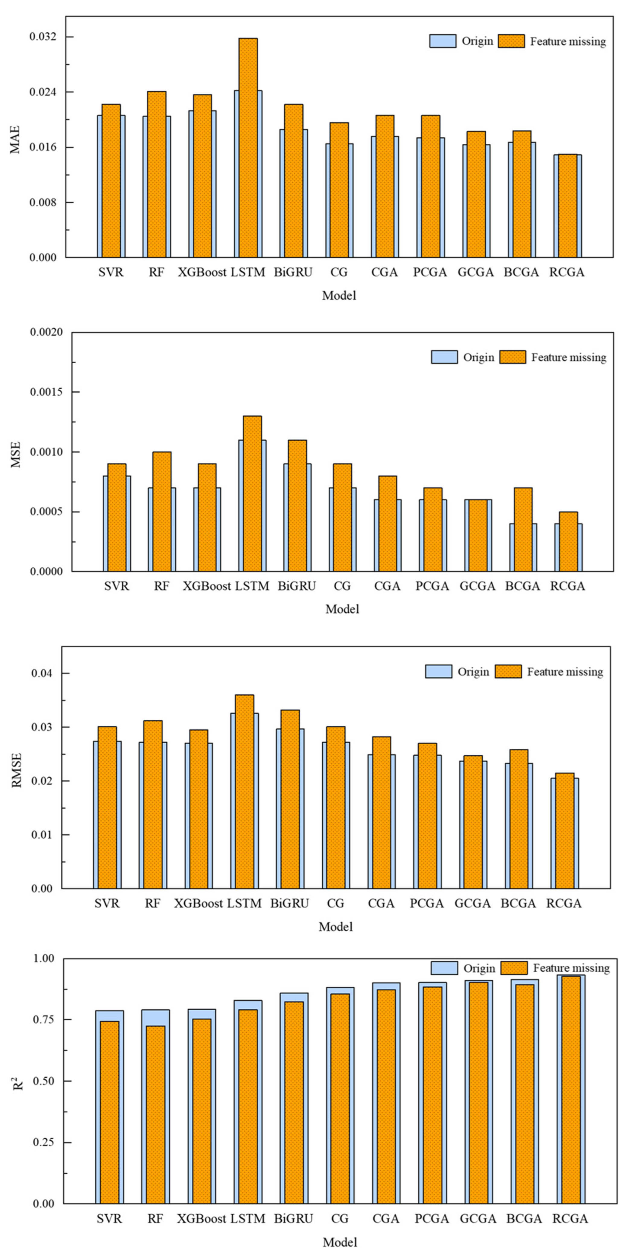
Sailing course is a key parameter in ship navigation and navigation control, with significant implications for route planning and collision avoidance operations. Given that aging ships frequently suffer from temporary COG data outages caused by sensor aging or intermittent communication disruptions, this section addresses the scenario of COG data deprivation for the model and evaluates the adaptability of the RCGA model in such a context. This section assumes a scenario in which such failures result in the complete loss of course over ground data and examines the adaptability of the RCGA model under these conditions. Course over ground is a core feature that reflects the navigation direction of the ship. The performance comparison of different models is shown in Figure 23. It can be observed that the absence of course data prevents the ML models from effectively capturing information related to changes in the navigation azimuth of the ship, resulting in various degrees of deterioration in the prediction performance of each model. While “F” indicates the equipment failure scenario with missing sailing course data, “O” stands for the original complete data scenario [49]. The performance of different models is presented in

Table 8. The performance comparison list of different models.

Model	Data Set	MAE	MSE	RMSE	R2
SVR	Origin	0.0206	0.0008	0.0274	0.7874
	Feature missing	0.0222	0.0009	0.0301	0.7433
RF	Origin	0.0205	0.0007	0.0272	0.7901
	Feature missing	0.0241	0.0010	0.0312	0.7251
XGBoost	Origin	0.0213	0.0007	0.0270	0.7932
	Feature missing	0.0236	0.0009	0.0295	0.7531
LSTM	Origin	0.0242	0.0011	0.0326	0.8289
	Feature missing	0.0318	0.0013	0.0360	0.7906
BiGRU	Origin	0.0186	0.0009	0.0297	0.8589
	Feature missing	0.0222	0.0011	0.0332	0.8238
CG	Origin	0.0165	0.0007	0.0272	0.8817
	Feature missing	0.0196	0.0009	0.0301	0.8556
CGA	Origin	0.0176	0.0006	0.0249	0.9010
	Feature missing	0.0206	0.0008	0.0282	0.8728
PCGA	Origin	0.0174	0.0006	0.0248	0.9018
	Feature missing	0.0206	0.0007	0.0270	0.8837
GCGA	Origin	0.0164	0.0006	0.0237	0.9106
	Feature missing	0.0183	0.0006	0.0247	0.9026
BCGA	Origin	0.0167	0.0005	0.0233	0.9130
	Feature missing	0.0184	0.0007	0.0258	0.8934
RCGA	Origin	0.0149	0.0004	0.0205	0.9330
	Feature missing	0.0150	0.0005	0.0215	0.9264

. It is evident that in the specific comparison of prediction performance across all models, the MAE, MSE, and RMSE of the RCGA model increased to 0.0150, 0.0005, and 0.0215, respectively, while the R² value decreased to 0.9264, representing only a 0.71% reduction. In contrast, the prediction errors of other models increased significantly. These results demonstrate that the RCGA model maintains strong adaptability and can achieve excellent prediction performance even in the absence of course data.

5.4. Discussions

This study proposes the RCGA model, which integrates the local feature extraction capability of the CNN, the bidirectional temporal modeling capability of the BiGRU, the dynamic feature weighting function of the multi-head attention mechanism, and the hyperparameter optimization capability of the ROA.

Regarding the experimental design, the study adopts an 8:2 temporal split to separate the training and test sets, which is reasonably justified for the application scenario of ship FC prediction on fixed routes. This splitting strategy allows for model training based on historical time-series data and performance evaluation on unseen real-world operational data collected after the training period, which can reflect the practical performance of the model on the target ship and route to a certain extent. However, it should be noted objectively that the dataset employed in this study is limited in scale and exhibits temporal autocorrelation, so the potential risk of model overfitting cannot be ruled out. Meanwhile, the current validation scheme is only implemented on a specific ship and fixed route, covering a narrow range of navigational operating conditions. As a result, it is insufficient to fully demonstrate the generalization capability of the model to unobserved operating conditions, alternative ships, or different routes.

To further improve the reliability and applicability of the proposed model, future work will introduce more comprehensive validation strategies. These include expanding datasets covering multiple ships and various routes to verify cross-vessel and cross-route generalization performance, adopting rolling horizon prediction to adapt to real-time application scenarios, and adding overfitting tests and extrapolation validation under different operating conditions, so as to enhance the robustness and reliability of the model in a wider range of maritime operational scenarios.

When considering computational requirements, the proposed model exhibits a reasonable training time, while both the number of parameters and the optimization overhead during inference are kept at a low level. This efficiency translates to strong deployment feasibility: shore-based decision-support systems, which typically have ample computational resources, can directly deploy the original model. In contrast, onboard systems with constrained resources can adopt a lightweight quantized version of the model to meet real-time performance requirements.

However, it is important to note a potential limitation of the proposed framework. The wind speed, a key input feature, is derived from vector synthesis, which means that measurement noise or deviations in the source vectors will propagate to the synthesized wind speed. This may introduce systematic deviations into the model input and consequently affect prediction accuracy, a point that will be addressed in future refinements.

To clarify the generalizability of our framework, we distinguish between scenario-specific and transferable components. Scenario-specific elements, such as vessel/route-dependent feature distributions and clustering thresholds, require recalibration when applied to new ships or routes. In contrast, inherently transferable components—including the ROA-driven attention mechanism and the hybrid CNN-BiGRU architecture—can be directly applied to other FC prediction tasks. To further validate this generalizability, we plan to extend our experiments to 2 additional bulk carriers, 3 coastal routes, and both coastal and open-water operating profiles.

Beyond the field of ship FC prediction, the RCGA model also demonstrates promising transferability to other domains facing similar challenges. For example, in the detection of subtle faults in operational air handling units (AHUs), the continuous temporal sensor data is analogous to ship FC time series [50]: the CNN extracts local features from sensor fluctuations, the BiGRU captures bidirectional temporal dependencies, and the attention mechanism locates critical fault-related segments, thereby addressing the challenge of detecting subtle fault patterns. Similarly, in the task of fire-door defect text detection, which involves sequential text data [51], the framework can be adapted to extract local text features via CNN, model contextual dependencies via BiGRU, and focus on defect-related keywords via the attention mechanism—effectively solving the difficulty of key feature extraction from unstructured text sequences.

6. Conclusions and Future Research Work

Based on real ship voyage data, this paper proposes an RCGA model for predicting ship FC. First, input features for the ship FC prediction model are selected using the Pearson correlation coefficient method and cluster analysis method. Concurrently, the ROA is employed to precisely tune key hyperparameters, including the Lr, the number of hidden units, and the L₂ coefficient. Subsequently, the model utilizes a CNN-BiGRU-Attention hybrid network to extract spatiotemporal features from multiple input data streams. An attention mechanism is incorporated to perform weighted fusion of key information, thereby significantly enhancing the model’s predictive capability. Through case study analysis and rigorous validation using actual voyage data, the results verify that the RCGA model significantly outshines traditional models such as SVR, RF, XGBoost, LSTM, and BiGRU, as well as other optimized variants, in terms of prediction accuracy. Specifically, the model achieves the highest goodness-of-fit (R² = 0.9330) and the lowest error level (RMSE = 0.0205). These results clearly indicate that the proposed model can accurately and stably predict FC during ship operations. Furthermore, the model exhibits superior robustness and stability, providing valuable high-precision data support for optimizing ship energy efficiency and enabling intelligent control. Therefore, the RCGA model contributes to improving ship energy efficiency and has positive implications for reducing carbon emissions during ship operation.

There are some limitations in the current model. On the one hand, the accuracy of sensors is not considered in this study, which may affect the dependability of the data. On the other hand, the generalization performance of the proposed model is limited, as it is only applicable to the target ship, and its applicability to other types of ships remains unknown. In future work, experimental analysis will be conducted based on the existing FC prediction model, incorporating more data from different types of ships and voyages, to improve the generalization performance of the model and expand its application scope. In future research, we will integrate physics-based constraints such as hull resistance and propeller efficiency models with our deep learning framework to enhance interpretability and incorporate additional operational features such as ROT, rudder activity, and slip, as well as hull/propeller condition monitoring data.

References

1. Review of Maritime Transport. 2024. Available online: https://unctad.org/publication/review-maritime-transport-2024 (accessed on 31 January 2026).
2. Fourth Greenhouse Gas Study. 2020. Available online: https://www.imo.org/en/ourwork/environment/pages/fourth-imo-greenhouse-gas-study-2020.aspx (accessed on 31 January 2026).
3. Li, Z.; Wang, K.; Liang, H.; Wang, Y.; Ma, R.; Cao, J.; Huang, L. Marine alternative fuels for shipping decarbonization: Technologies, applications and challenges. Energy Convers. Manag. 2025, 329, 119641. [Google Scholar] [CrossRef] [Scilit]
4. Cai, Z.; Li, L.; Yu, L.; Li, C.; Sun, M. Diversity, quality, and quantity of real ship data on the black-box and gray-box prediction models of ship fuel consumption. Ocean Eng. 2024, 291, 116434. [Google Scholar] [CrossRef] [Scilit]
5. Duan, M.; Wang, Y.; Fan, A.; Yang, J.; Fan, X. Comprehensive analysis and evaluation of ship energy efficiency practices. Ocean Coast. Manag. 2023, 231, 106397. [Google Scholar] [CrossRef] [Scilit]
6. Guidelines for Voluntary Use of the Ship Energy Efficiency Operational Indicator (EEOI). Available online: https://www.classnk.or.jp/hp/pdf/activities/statutory/eedi/mepc_1-circ_684.pdf (accessed on 31 January 2026).
7. DNV. Ship Energy Efficiency Management Plan (SEEMP): Development and Implementation. Available online: https://www.dnv.com/maritime/hub/decarbonize-shipping/key-drivers/regulations/imo-regulations/seemp/ (accessed on 31 January 2026).
8. Yuan, Z.; Liu, J.; Zhang, Q.; Liu, Y.; Yuan, Y.; Li, Z. Prediction and optimisation of fuel consumption for inland ships considering real-time status and environmental factors. Ocean Eng. 2021, 221, 108530. [Google Scholar] [CrossRef] [Scilit]
9. Yan, R.; Wang, S.; Du, Y. Development of a two-stage ship fuel consumption prediction and reduction model for a dry bulk ship. Transp. Res. Part E Logist. Transp. Rev. 2020, 138, 101930. [Google Scholar] [CrossRef] [Scilit]
10. Li, X.; Sun, B.; Jin, J.; Ding, J. Speed Optimization of Container Ship Considering Route Segmentation and Weather Data Loading: Turning Point-Time Segmentation Method. J. Mar. Sci. Eng. 2022, 10, 1835. [Google Scholar] [CrossRef] [Scilit]
11. Li, Z.; Wang, K.; Hua, Y.; Liu, X.; Ma, R.; Wang, Z.; Huang, L. GA-LSTM and NSGA-III based collaborative optimization of ship energy efficiency for low-carbon shipping. Ocean Eng. 2024, 312, 119190. [Google Scholar] [CrossRef] [Scilit]
12. Du, Y.; Meng, Q.; Wang, S.; Kuang, H. Two-phase optimal solutions for ship speed and trim optimization over a voyage using voyage report data. Transp. Res. Part B Methodol. 2019, 122, 88–114. [Google Scholar] [CrossRef] [Scilit]
13. Wang, K.; Li, Z.; Zhang, R.; Ma, R.; Huang, L.; Wang, Z.; Jiang, X. Computational fluid dynamics-based ship energy-saving technologies: A comprehensive review. Renew. Sustain. Energy Rev. 2025, 207, 114896. [Google Scholar] [CrossRef] [Scilit]
14. Wang, K.; Li, Z.; Liu, X.; Hu, Z.; Huang, L.; Song, Q.; Liang, H.; Jiang, X. Wind-assisted propulsion system for shipping decarbonization: Technologies, applications and challenges. Energy 2025, 336, 138420. [Google Scholar] [CrossRef] [Scilit]
15. Li, Z.; Wang, K.; Liu, Y.; Liang, H.; Zhang, D.; Wang, Z.; Cao, J.; Huang, L. Evaluation of energy-saving effects of a wing-typed sail-assisted ship using wind energy density route analysis. Ocean Eng. 2026, 345, 123693. [Google Scholar] [CrossRef] [Scilit]
16. Wang, K.; Liu, X.; Guo, X.; Wang, J.; Wang, Z.; Huang, L. A novel high-precision and self-adaptive prediction method for ship energy consumption based on the multi-model fusion approach. Energy 2024, 310, 133265. [Google Scholar] [CrossRef] [Scilit]
17. Luo, X.; Yan, R.; Wang, S. Ship sailing speed optimization considering dynamic meteorological conditions. Transp. Res. Part C Emerg. Technol. 2024, 167, 104827. [Google Scholar] [CrossRef] [Scilit]
18. Ma, W.; Han, Y.; Tang, H.; Ma, D.; Zheng, H.; Zhang, Y. Ship route planning based on intelligent mapping swarm optimization. Comput. Ind. Eng. 2023, 176, 108920. [Google Scholar] [CrossRef] [Scilit]
19. Wang, K.; Wang, Y.; Liang, H.; Jing, Z.; Cong, L.; Ma, R.; Huang, L. Ship energy efficiency optimization considering the influences of multiple complex navigational environments: A review. Mar. Pollut. Bull. 2025, 216, 117976. [Google Scholar] [CrossRef] [Scilit] [PubMed]
20. Wang, K.; Cong, L.; Jing, Z.; Li, Z.; Wang, Y.; Chi, Y.; Liang, H. Artificial intelligence and machine learning for green and intelligent shipping: Methods, applications and challenges. Comput. Ind. Eng. 2026, 211, 111647. [Google Scholar] [CrossRef] [Scilit]
21. Vorkapić, A.; Radonja, R.; Martinčić-Ipšić, S. Predicting Seagoing Ship Energy Efficiency from the Operational Data. Sensors 2021, 21, 2832. [Google Scholar] [CrossRef] [Scilit]
22. Xie, X.; Sun, B.; Li, X.; Zhao, Y.; Chen, Y. Joint optimization of ship speed and trim based on machine learning method under consideration of load. Ocean Eng. 2023, 287, 115917. [Google Scholar] [CrossRef] [Scilit]
23. Yang, H.; Sun, Z.; Han, P.; Ma, M. Data-driven prediction of ship fuel oil consumption based on machine learning models considering meteorological factors. Proc. Inst. Mech. Eng. Part M J. Eng. Marit. Environ. 2024, 238, 483–502. [Google Scholar] [CrossRef] [Scilit]
24. Park, M.H.; Lee, C.H.; Hur, J.J.; Lee, W.J. Prediction of fuel consumption and shaft torque using machine learning and analysis of engine curve diagrams. Measurement 2025, 248, 116984. [Google Scholar] [CrossRef] [Scilit]
25. Xia, M.; Fan, A.; Hu, Z.; Vladimir, N.; Mao, W. Data augmentation-based approach to enhance the accuracy, generalization, and reliability of ship fuel consumption prediction. Ocean Eng. 2025, 341, 122558. [Google Scholar] [CrossRef] [Scilit]
26. Tzortzis, G.; Sakalis, G. A dynamic ship speed optimization method with time horizon segmentation. Ocean Eng. 2021, 226, 108840. [Google Scholar] [CrossRef] [Scilit]
27. Piercey, C.; Hamilton, M.; Veitch, B.; Barnes, J.; Jiang, X. Ship Data Clustering for Improved Fuel Efficiency Optimization Decision Support Systems. In Proceedings of the OCEANS 2024-Halifax, Halifax, NS, Canada, 23–26 September 2024; IEEE: New York, NY, USA; pp. 1–6.
28. Yan, X.; Wang, K.; Yuan, Y.; Jiang, X.; Negenborn, R.R. Energy-efficient shipping: An application of big data analysis for optimizing engine speed of inland ships considering multiple environmental factors. Ocean Eng. 2018, 169, 457–468. [Google Scholar] [CrossRef] [Scilit]
29. Wang, L.; Chen, P.; Chen, L.; Mou, J. Ship AIS Trajectory Clustering: An HDBSCAN-Based Approach. J. Mar. Sci. Eng. 2021, 9, 566. [Google Scholar] [CrossRef] [Scilit]
30. Liu, L.; Zhang, Y.; Hu, Y.; Wang, Y.; Sun, J.; Dong, X. A Hybrid-Clustering Model of Ship Trajectories for Maritime Traffic Patterns Analysis in Port Area. J. Mar. Sci. Eng. 2022, 10, 342. [Google Scholar] [CrossRef] [Scilit]
31. Wang, K.; Hua, Y.; Huang, L.; Guo, X.; Liu, X.; Ma, Z.; Ma, R.; Jiang, X. A novel GA-LSTM-based prediction method of ship energy usage based on the characteristics analysis of operational data. Energy 2023, 282, 128910. [Google Scholar] [CrossRef] [Scilit]
32. Hu, C.; Wang, Y.; Zhou, B.; Han, X.; Yi, W.; Zhang, G. Extended period time series prediction of adaptive gray-box fuel consumption for variable pitch ships based on ET-Informer. Ocean Eng. 2025, 339, 121939. [Google Scholar] [CrossRef] [Scilit]
33. Zhong, W.; Bai, K.; Gu, Y.; Ye, N. Ship fuel consumption prediction based on ResGCN and iLSTM with multi-scale dynamic attention mechanism. Ocean Eng. 2026, 343, 123191. [Google Scholar] [CrossRef] [Scilit]
34. Li, X.; Zuo, Y.; Li, T.; Chen, C.L.P. A Novel Machine Learning Model Using CNN-LSTM Parallel Networks for Predicting Ship Fuel Consumption. In Neural Information Processing; Springer Nature: Singapore, 2024; pp. 108–118. [Google Scholar]
35. Wang, K.; Wang, J.; Huang, L.; Yuan, Y.; Wu, G.; Xing, H.; Wang, Z.; Wang, Z.; Jiang, X. A comprehensive review on the prediction of ship energy consumption and pollution gas emissions. Ocean Eng. 2022, 266, 112826. [Google Scholar] [CrossRef] [Scilit]
36. Dianyu, E.; Zhang, Y.; Hu, H.; Xu, G.; Liu, L.; Cui, J.; Tan, C.; Zou, R.; Kuang, S. CFD data-driven CNN-LSTM for fast prediction of instantaneous flow characteristics in hydrocyclones. Miner. Eng. 2026, 235, 109814. [Google Scholar]
37. Han, P.; Liu, Z.; Li, C.; Sun, Z.; Yan, C. A novel federated learning-based two-stage approach for ship energy consumption optimization considering both shipping data security and statistical heterogeneity. Energy 2024, 309, 133150. [Google Scholar] [CrossRef] [Scilit]
38. Zhou, X.; Yang, X.; Zhou, M.; Liu, L.; Niu, S.; Zhou, C.; Wang, Y. Multi-Temporal Energy Management Strategy for Fuel Cell Ships Considering Power Source Lifespan Decay Synergy. J. Mar. Sci. Eng. 2025, 13, 34. [Google Scholar] [CrossRef] [Scilit]
39. Fang, S.; Shu, S.; Pan, J.; Huang, H.; Wang, G.; Wang, K. A long-term and short-term prediction method for power transformer top oil temperature based on comprehensive thermal factor and CNN-LSTM-attention. Int. J. Electr. Power Energy Syst. 2025, 172, 111170. [Google Scholar] [CrossRef] [Scilit]
40. Quan, R.; Cheng, G.; Guan, X.; Zhang, G.; Quan, J. A HO-BiGRU-Transformer based PEMFC degradation prediction method under different current conditions. Renew. Energy 2026, 256, 124132. [Google Scholar] [CrossRef] [Scilit]
41. Yang, X.; Peng, S.; Zhang, Z.; Du, Y.; Linghu, L. Thermal error prediction in dry hobbing machine tools: A CNN-BiGRU network with spatiotemporal feature fusion. Measurement 2025, 256, 118389. [Google Scholar] [CrossRef] [Scilit]
42. Shrestha, A.; Mahmood, A. Review of Deep Learning Algorithms and Architectures. IEEE Access 2019, 7, 53040–53065. [Google Scholar] [CrossRef] [Scilit]
43. Song, E.; Zhang, X.; Ge, Y.; Yao, C.; Wang, B. Parallel TCN-BiGRU architecture with dynamic attention for ship energy consumption prediction under variable navigation conditions. Energy 2025, 337, 138601. [Google Scholar] [CrossRef] [Scilit]
44. Liu, Y.; Wang, K.; Lu, Y.; Zhang, Y.; Li, Z.; Ma, R.; Huang, L. A Ship Energy Consumption Prediction Method Based on TGMA Model and Feature Selection. J. Mar. Sci. Eng. 2024, 12, 1098. [Google Scholar] [CrossRef] [Scilit]
45. Raeisi Gahrouei, J.; Beheshti, Z. The Electricity Consumption Prediction using Hybrid Red Kite Optimization Algorithm with Multi-Layer Perceptron Neural Network. J. Intell. Proced. Electr. Technol. 2022, 15, 1–22. [Google Scholar]
46. Li, D.; Cheng, B.; Xiang, S. Direct cubic B-spline interpolation: A fuzzy interpolating method for weightless, robust and accurate DVC computation. Opt. Lasers Eng. 2024, 172, 107886. [Google Scholar] [CrossRef] [Scilit]
47. Wang, N.; Kong, X.; Ren, B.; Hao, L.; Han, B. SeaBil: Self-attention-weighted ultrashort-term deep learning prediction of ship maneuvering motion. Ocean Eng. 2023, 287, 115890. [Google Scholar] [CrossRef] [Scilit]
48. Li, Z.; Wang, K.; Ruan, Z.; Li, D.; Liang, H.; Ma, R.; Cao, J.; Huang, L. A fuel consumption prediction model for wind-assisted ship based on operational data. Transp. Res. Part Transp. Environ. 2025, 149, 105045. [Google Scholar] [CrossRef] [Scilit]
49. Lan, T.; Huang, L.; Ma, R.; Wang, K.; Ruan, Z.; Wu, J.; Li, X.; Chen, L. A robust method of dual adaptive prediction for ship fuel consumption based on polymorphic particle swarm algorithm driven. Appl. Energy 2025, 379, 124911. [Google Scholar] [CrossRef] [Scilit]
50. Wang, S. Real operational labeled data of air handling units from office, auditorium, and hospital buildings. Sci. Data 2025, 12, 1481. [Google Scholar] [CrossRef] [Scilit] [PubMed]
51. Wang, S.; Moon, S.; Eum, I.; Hwang, D.; Kim, J. A text dataset of fire door defects for pre-delivery inspections of apartments during the construction stage. Data Brief 2025, 60, 111536. [Google Scholar] [CrossRef] [Scilit] [PubMed]
Figure 1. The technical roadmap of the proposed RCGA model.
Jmse 14 00324 g001
Figure 2. Gated Recurrent Unit architecture.
Jmse 14 00324 g002
Figure 3. Bidirectional Gated Recurrent Unit architecture.
Jmse 14 00324 g003
Figure 4. Schematic diagram of multi-head self-attention.
Jmse 14 00324 g004
Figure 5. The movement of each red kite in the ROA.
Jmse 14 00324 g005
Figure 6. The diagram of the sailing route.
Jmse 14 00324 g006
Figure 7. The process of data acquisition.
Jmse 14 00324 g007
Figure 8. The distribution of environmental characteristics and FC.
Jmse 14 00324 g008
Figure 9. Pearson correlation analysis.
Jmse 14 00324 g009
Figure 10. The related data distribution of the target sailing route.
Jmse 14 00324 g010
Figure 11. DBSCAN-based clustering result visualization.
Jmse 14 00324 g011
Figure 12. The framework of the proposed model.
Jmse 14 00324 g012
Figure 13. Prediction results of the RCGA model.
Jmse 14 00324 g013
Figure 14. Scatter plots of the distribution of each prediction model results.
Jmse 14 00324 g014
Figure 15. Quantitative comparison of model performance metrics.
Jmse 14 00324 g015
Figure 16. Radar chart comparison of prediction performance across different models.
Jmse 14 00324 g016
Figure 17. The performance comparison of different models.
Jmse 14 00324 g017
Figure 18. Time series plots of model residuals.
Jmse 14 00324 g018
Figure 19. Histogram plots of model residuals.
Jmse 14 00324 g019
Figure 20. The diagram of the semi-violin and semi-boxplot.
Jmse 14 00324 g020
Figure 21. The comparison between Gaussian noise data and the original data.
Jmse 14 00324 g021
Figure 22. The performance comparison of different models.
Jmse 14 00324 g022
Figure 23. The performance comparison of different models.
Jmse 14 00324 g023