Article

Modeling Air–Sea Turbulent Fluxes: Sensitivity to Surface Roughness Parameterizations

1
School of Hydraulic and Ocean Engineering, Changsha University of Science & Technology, Changsha 414004, China
2
College of Meteorology and Oceanography, National University of Defense Technology, Changsha 410073, China
3
Key Laboratory of Water-Sediment Sciences and Water Disaster Prevention of Hunan Province, Changsha 414004, China
4
Key Laboratory of Dongting Lake Aquatic Eco-Environmental Control and Restoration of Hunan Province, Changsha 414004, China
*
Authors to whom correspondence should be addressed.
J. Mar. Sci. Eng. 2026, 14(3), 277; https://doi.org/10.3390/jmse14030277
Submission received: 12 December 2025 / Revised: 7 January 2026 / Accepted: 19 January 2026 / Published: 29 January 2026
(This article belongs to the Topic Advances in Environmental Hydraulics, 2nd Edition)

Abstract

During tropical cyclones (TCs), intense exchanges of momentum, heat, and moisture occur across the air–sea interface. The present study was conducted to investigate the role of surface roughness parameterizations under such conditions. To this end, a series of sensitivity experiments was conducted with a focus on Tropical Cyclone Biparjoy, which originated from the Indian Ocean in 2023. The experiments evaluate the impact of different schemes for momentum, thermal, and moisture roughness length on TC track, intensity, significant wave height, and air–sea heat fluxes. The results indicate that the momentum roughness length scheme is critical for accurately forecasting TC track and intensity and for simulating significant wave height; furthermore, Drennan’s parameterization yielded slightly better results in this case, with the smallest track error (72.0 km MAE) among the momentum schemes. Under the premise that Drennan’s parameterization scheme has high accuracy in momentum roughness, sensitivity experiments on thermal and moisture roughness parameterization were conducted. The Drennan–Fairall2014 combination achieved the lowest errors in TC central pressure (4.25 hPa RMSE) and the maximum sustained wind speed (5.31 m/s RMSE). Thermal and moisture roughness mainly affects the efficiency of turbulent heat transfer between the ocean and the atmosphere and thus has a limited impact on the cooling of sea surface temperature, with SST RMSE differences among schemes within 0.3 °C. This effect is mainly confined to the uppermost ocean layer and does not significantly change the thermal structure of the upper layers.

1. Introduction

Tropical cyclones (TCs), also known as hurricanes or typhoons in different regions, generate and develop over the tropical or subtropical ocean surface. These powerful weather systems significantly impact the marine environment and atmospheric system while also leading to serious human casualties and heavy losses of property in coastal areas during landing.
During TC periods, intense exchanges of heat, momentum, and material occur at the air–sea interface. The wind stress generated by TCs influences ocean currents and induces storm surges, while the ocean, in turn, affects TC development through processes such as heat transfer and water vapor exchange.
Therefore, investigating the mechanism of heat, momentum, and material exchange between TCs and the ocean is crucial for enhancing our understanding of TCs and improving the accuracy of TC predictions, thereby aiding in the effective mitigation of the impacts of these adverse weather events [1].
Due to the lack of observations under TC conditions, our understanding of the air–sea interaction during a TC largely relies on numerical simulation [2]. Numerical modeling has become a crucial approach in the study and prediction of TCs. The accurate depiction of processes occurring below the model’s grid scale is of paramount importance for numerical weather prediction. Since these processes cannot be directly resolved by model dynamics, they must be represented through parameterization schemes, a necessity highlighted by Bauer et al. [3].
Among these physical processes, the calculation of surface momentum and enthalpy fluxes significantly influences TC intensity simulation, and the estimation of these fluxes highly depends on the parameterization of surface roughness, particularly the momentum, thermal, and moisture roughness length (z0, zt, zq). Different parameterization schemes can substantially affect the drag coefficient (Cd) and enthalpy exchange coefficient (Ck), thereby modulating the vertical transport of energy and momentum, which ultimately impacts the simulated structure and intensity of TCs.
In the past, Charnock [4] had stated that the drag coefficient generally increases from about 0.001 to 0.003 for TCs with ordinary intensity, and it can increase to 0.005 for TCs with a wind speed > 70 ms−1. However, recent field observations and laboratory experiments [5,6] found that Cd reaches a maximum of about 0.003 for TCs with wind speeds from 30 to 40 ms−1. Emanuel [7] suggested that the ratio of enthalpy to momentum exchange coefficients in real hurricanes lies in the range between 0.75 and 1.5. This result contradicts previous thinking about the behavior of the heat and momentum exchange coefficients at high wind speed [8]. Recent studies have reached differing conclusions about the likely value of Ck/Cd for high wind speeds on the basis of numerical simulations [9,10]. Bryan [10] suggested that this difference in values may be due to the relatively large horizontal diffusion and low sea surface temperature (SST) used by Emanuel [7]. The TC process is a complex set of ocean–atmosphere–wave coupling processes. Davis et al. [11] and Chen et al. [12] reported that the best method for the determination of the real drag coefficient over the sea surface is wave modeling. Recent advancements have further detailed the multifaceted role of waves. Wave states and associated phenomena critically govern momentum transfer. Alimohammadi et al. [13] used the WRF-SWAN coupled model (COAWST) to compare the effects of various momentum roughness length parameterizations in simulating Tropical Cyclone Gonu. They found that the Oost [14] scheme led to a significant overestimation of roughness length, while the Drennan [15] and Taylor [16] schemes yielded more realistic results. The choice of parameterization had a much greater impact on the simulated maximum wind speed than on the central pressure, highlighting the critical role of momentum roughness in modulating wind intensity. Building upon such comparative studies, novel parameterizations are now being developed for direct implementation in operational forecasting and climate models. A prominent example is the wave-age-dependent stress parameterization (WASP) by Bouin et al. [17], which is designed for the SURFEX surface model and used in Météo-France’s operational systems. WASP integrates the effect of wave growth on wind stress and is calibrated against a vast set of observations, ensuring the accurate representation of turbulent fluxes across a wide wind speed range, including tropical cyclone conditions. Zhao et al. [18] developed a novel drag parameterization that simultaneously considers wave age, wave steepness, and sea spray stress, revealing the complex behavior of the effective drag coefficient under varying wind and wave conditions. Collectively, these studies highlight that advancing TC simulation accuracy necessitates coupled modeling systems capable of integrating these sophisticated representations of both wave-driven thermal and momentum fluxes.
In addition to momentum exchange, the accurate parameterization of thermal and moisture roughness lengths is equally critical, as they directly govern the sensible and latent heat fluxes that affect tropical cyclone development. Following the establishment of the COARE 3.0 algorithm [19], which provided a unified and observationally constrained framework for scalar roughness lengths, the core parameterizations for these quantities under low-to-moderate wind conditions have been considered relatively mature. Subsequent research efforts have largely shifted towards refining these schemes for extreme high-wind environments, particularly by incorporating the complex effects of sea spray [18,20,21]. However, the parameterizations of spray-mediated fluxes remain diverse and without a clear consensus, introducing significant uncertainty. Given the current lack of consensus and high uncertainty in sea spray parameterization schemes, and to maintain a clear focus on isolating the effects of fundamental surface roughness processes, this work deliberately employs traditional parameterizations for thermal and moisture roughness lengths. This approach allows for a more interpretable attribution of model sensitivities to the core parameterizations under investigation.
Therefore, selecting appropriate roughness length parameterizations is essential for improving the accuracy of tropical cyclone simulations. The main purpose of this research is to define which one of the parameterizations presented by Taylor and Yelland [16], Drennan et al. [15], Oost et al. [14], and Edson et al. [22] for calculating momentum roughness length at the sea surface introduced in Section 2.1 is close to reality. Alimohammadi et al. [13] suggested that employing persistent online coupling among the atmosphere, ocean, and wave models throughout the TC life cycle would better capture SST cooling and is expected to significantly enhance the simulation results beyond those achieved with WRF-SWAN coupling alone. So it is significant to introduce the ROMS model to construct a fully coupled COAWST model for ROMS–WRF–SWAN. A key mechanism behind this SST cooling is the role of wave-breaking processes in modulating the upper ocean thermal structure. For instance, Cao et al. [23] demonstrated that a new wave-breaking parameterization strengthened turbulent mixing under typhoon conditions, leading to a notable SST decrease. Recent studies have shown that the advantage of such fully coupled models lies in their more physically consistent representation of air–sea interaction processes [24,25]. With the predicted SST from the coupled ocean model, the thermal radiation process and heat flux exchange between the ocean and the atmosphere can be more accurately simulated.
Another purpose of this research is to investigate the impact of thermal and moisture roughness lengths on heat fluxes and tropical cyclone intensity by conducting sensitivity experiments with different parameterization schemes. Our sensitivity experiments are thus designed to isolate and quantify the impact of these established but crucial scalar roughness length schemes on heat fluxes and, importantly, on the subsequent response of the upper ocean structure.
The upper layer response to different roughness length parameterization schemes was analyzed using data from the Operational Sea Surface Temperature and Sea Ice Analysis (OSTIA) system, Jason-3 satellite altimeter, and Argo floats. The features of heat were described and compared to the ERA5 climate dataset. In Section 2, the theory and formula of different roughness length parameterization schemes are described, and the experiment area, the coupled model descriptions, the formation of TC Biparjoy, and the validation data are outlined. Section 3 details the parametric verification and presents the simulation results. Section 4 discusses the findings in light of this study’s limitations and uncertainties. Finally, this paper concludes with a summary and an outline of potential future research directions in Section 5.

2. Materials and Methods

2.1. Model Descriptions

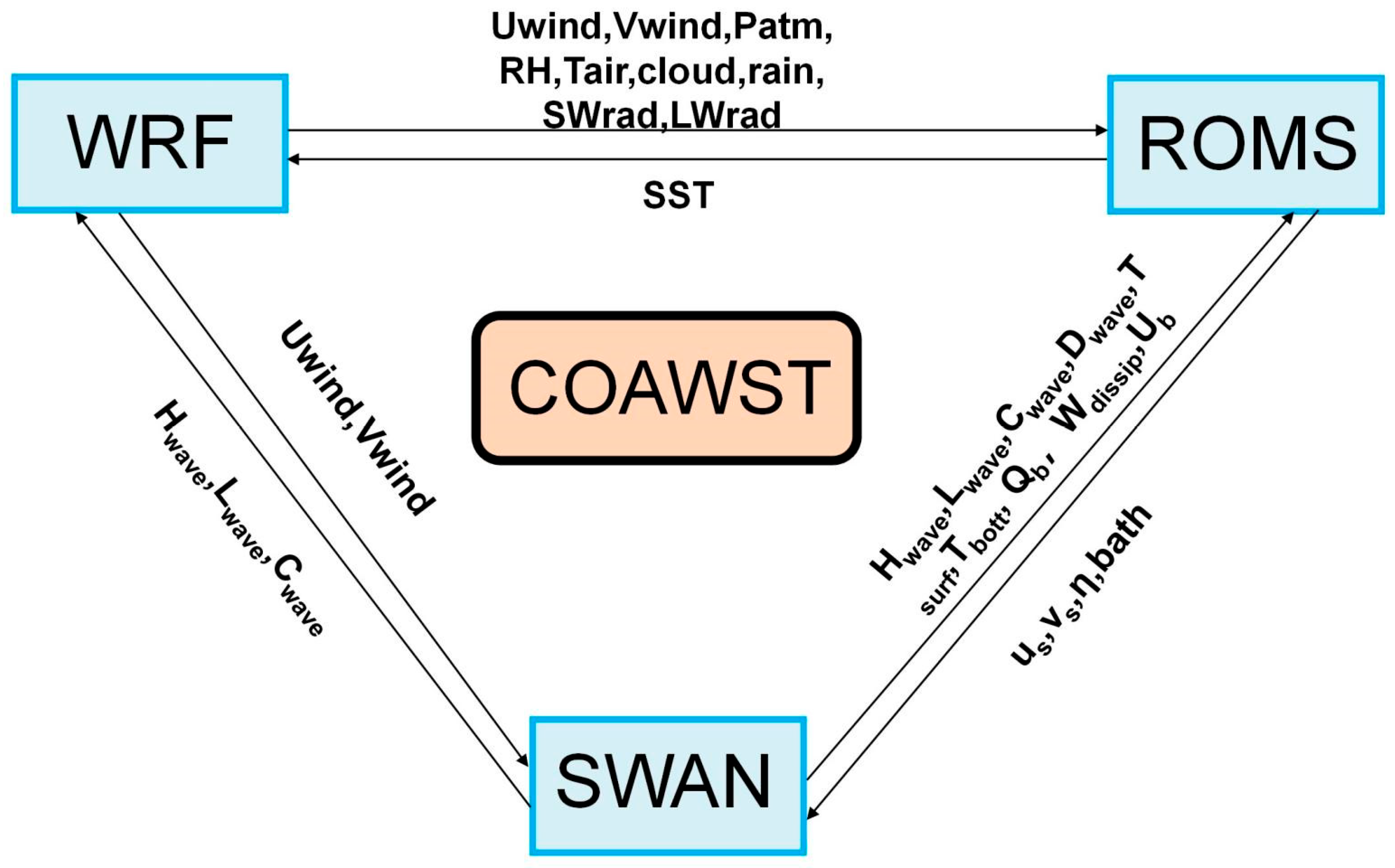
A coupled atmosphere–ocean–wave model, as a part of the ‘Coupled Ocean-Atmosphere-Wave-Sediment Transport’ (COAWST3.8) modeling system [26], was used in this study. The ‘model coupling toolkit’ (MCT) was used to couple the atmosphere–ocean–wave model Weather Research and Forecasting Model (WRF), the ocean model Regional Ocean Modelling System (ROMS), and The Simulating Waves Nearshore (SWAN) model. The main advantage of the COAWST model is its ability to simulate multiscale and multiphysical processes, making it suitable for studying marine climate, extreme weather events, and their impact on marine ecosystems. Through real-time coupling, as shown in Figure 1, the model can more accurately capture the response of ocean surface wind fields, temperatures, and flows to climate change.
The WRF model is a quasi-compressible, non-hydrostatic model. As a widely used mesoscale numerical model for both research and operational forecasting, WRF offers multiple physical parameterization schemes and a configurable dynamic framework, enabling the relatively accurate simulation of TC track and intensity evolution. It incorporates various planetary boundary layer schemes, microphysical processes, radiation schemes, and surface flux parameterizations to represent complex air–sea interactions. The WRF calculation area covers the Bay of Bengal, Andaman Sea, and Palk Strait. A single-domain setup was used for the study area, with a horizontal resolution of 9 km. The model consisted of 45 vertical levels, with the top boundary pressure set to 50 hPa and time step set to 45 s. The parameterization scheme is shown in Table 1.
ROMS, developed by Rutgers University in the United States, is an ocean general circulation model, which is a three-dimensional, free-surface, non-linear model. The ROMS main grid is located within the WRF main grid, with a spatial range of 3–27° N, 61–79° E. The resolution of the main grid is 6 km, and the vertical layering of the grid consists of 40 layers. Considering the simulation area, the northern boundary is set as the closed boundary and the rest as the open boundary. Coordinate control parameters are THETA_S = 8 and THETA_B = 0.1. The time step dt is 30 s. The vertical mixing physics used in the model considers the Generic Length Scale [33,34]. This study was conducted using E.U. Copernicus Marine Service Information (https://doi.org/10.48670/moi-00016). The initial and boundary conditions of the model are derived from Copernicus Marine Service, and the bathymetric data in the ROMS model are derived from the GEBCO bathymetric dataset [35].
The SWAN model solves the spectral density evolution equation to simulate wind wave generation and propagation in coastal waters [1]. ERA5 wind farm drive was used for individual SWAN simulations (UTC time for 5 days from 00:00, 1 June 2023 to 00:00, 6 June 2023) to provide hotfiles for coupled models. The time step dt is 360 s.
The coupling model simulation time was used to select the UTC time for 11 days from 00:00, 6 June 2023 to 00:00, 17 June 2023. The coupling mode exchanges data once every 270 s via the MCT. As shown in Table 2, six numerical experiments were conducted according to different schemes of momentum, thermal, and moisture roughness lengths.
We used three main statistical parameters—the mean absolute error (MAE), mean absolute percentage error (MAPE), and root mean square error (RMSE)—to assess the model’s simulation accuracy [38,39].
These parameters are calculated as follows:
M A E = 1 N i = 1 N | ( y i x i ) |
M A P E = 1 N i = 1 N | ( y i x i ) x i |
R M S E = 1 N i = 1 N ( y i x i ) 2  
where xi and yi represent the observed and simulated values, respectively. N represents the number of data points.

2.2. Roughness Length Parameterization Scheme

The WRF model uses the following parameterizations to calculate the surface fluxes for all selected schemes:
H = ρ C p C H U L ( S S T T L )
E = ρ L v C Q U L ( q 0 q L )
τ = ρ C D U L 2  
where H, E, and τ represent the sensible heat flux, latent heat flux, and momentum flux, respectively. UL, TL, and qL are the wind speed, air temperature, and water vapor mixing ratio at the lowest model level, respectively; Lv is the latent heat of vaporization; and Cp is the specific heat of air at constant pressure. ρ is the density of air, and q0 is the saturation water vapor mixing ratio at the SST; CH, CQ, and CD are the dimensionless coefficients of sensible heat, latent heat, and momentum exchange, respectively.
The total enthalpy flux, QK, is defined as follows:
Q K = ρ C k U L ( k 0 k L )
where Ck is the enthalpy exchange coefficient, and the enthalpy of moist air, k, is defined as follows:
k = [ ( 1 q ) C p a + q C p l ] + q L v  
where Cpa and Cpl are the specific heats of dry air and liquid water, respectively. q is the specific humidity.
The ambiguous parameters in the mentioned fluxes are drag and enthalpy exchange coefficients. These coefficients under neutral stability conditions follow
C d = K 2 [ ln ( z r e f z 0 ) ] 2
C h = K 2 [ ln ( z r e f z 0 ) ] × [ ln ( z r e f z T ) ] = C D 1 2 × K ln ( z r e f z T )
C q = K 2 [ ln ( z r e f z 0 ) ] × [ ln ( z r e f z Q ) ] =   C D 1 2 × K ln ( z r e f z Q )
where k (=0.40) is the von Karman constant, and zref is the reference height (zref in WRF is the lowest model level). The exchange coefficients of Cd, Ch, and Cq directly relate to the roughness lengths of momentum z0, sensible heat zt, and latent heat zq.
Some studies link zt and zq with the momentum roughness of the sea surface. Based on Surface Renewal Theory, Liu et al. [8] proposed the following formula:
z T u * ν = a 1 R r b 1
z Q u * ν = a 2 R r b 2
where ν is the kinematic viscosity of air. Rr is the roughness Reynolds number. a1, b1, a2, and b2 take different values based on the range of Rr.
The calculation scheme of zt and zq was used in COARE (Coupled Ocean Atmosphere Response Experiment) 2.5 [40]. After that, COARE3.0 was proposed by Fairall et al. [19]. zt = zq is assumed. Similarly, zt and zq can be expressed as functions of Rr:
z T = z Q = m i n ( 1.0 × 10 4 , 5.5 × 10 5 R r 0.6 )  
The scheme of COARE3.0 was verified in [41]. The COARE3.5 version used in this study was obtained from the source code of the MYNN surface layer scheme of the COAWST/WRF modeling system [26]. This implementation includes adjustments to the upper limits of zt and zq that originate from the work of Fairall2014, which are embedded in the model code but not separately published:
z T   =   z Q = m i n ( 1.6 × 10 4 , 5.8 × 10 5 R r 0.72 )
In addition to directly representing zt and zq as functions of Rr, another type of scheme [36,37] represents the ratio of zt and zq to z0 as a function of Rr:
z T =   z 0 e x p [ 2 ( 2.48 R e * 0.25 ) ]
z Q = z 0 e x p [ 2 ( 2.28 R e * 0.25 ) ]
where Re* is the roughness Reynolds number.
Most parameterization schemes represent Cd as a function of U10 (wind speed at 10 m height). In this study, the momentum parameterization scheme based on wind adopts Edson et al. [22], based upon the results of Donelan et al. [6], and its calculation formula is as follows:
z 0 = γ ν u * + C h u * 2 g
z 0 = m a x [ 1.27 × 10 7 , m i n ( z 0 , 2.85 × 10 3 ) ]
where ν is the kinematic viscosity of air. In the COARE3.5 scheme, γ is set to 0.11. u is the friction velocity. Ch is the Charnock coefficient. The Charnock coefficient Ch is represented as a function of wind speed (Ch = 0.017 U10 − 0.005).
Wave age and wave steepness are two key parameters describing sea surface properties and the wind wave development stage. When coupling the WRF model with the SWAN model within the COAWST platform, methods for determining the sea surface momentum roughness length via wave age and wave steepness can be implemented. Three parameterizations were also adopted in this study.
The first parameterization presented by Taylor and Yelland [16] is as follows:
z 0 H s = 1200 ( H s L p ) 4.5
where Lp is the wavelength at the peak of the wave spectrum, Hs is the significant wave height (SWH), and z0 is the momentum roughness length.
The second parameterization presented by Drennan et al. [15] is as follows:
z 0 H s = 3.35 ( U * C p ) 3.4
where Cp represents the wave phase speed at the peak frequence.
The third parameterization presented by Oost et al. [14] is as follows:
z 0 L p = 25.0 π ( U * C p ) 4.5
Warner et al. [26] used the drag Davis limiter [18] in order to limit the Oost, Taylor, and Drennan parameterizations. As recommended in the model, the Davis limiter is used in momentum parameterizations based on wave parameters by defining DRAGLIM_DAVIS.
z 0 = m i n ( z 0 , 2.85 × 10 3 )

2.3. TC Biparjoy

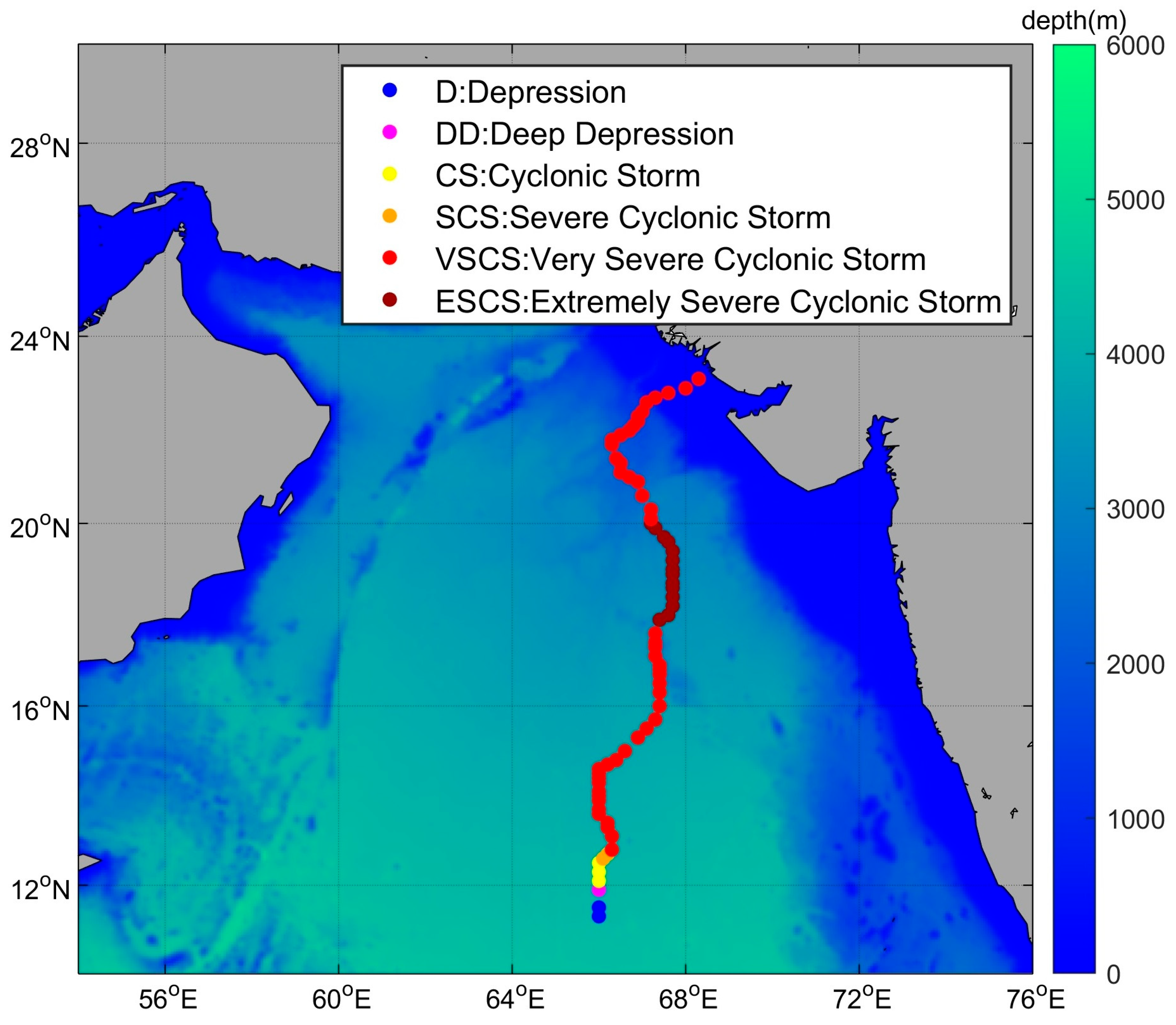
Cyclone Biparjoy formed over the southeast Arabian Sea on 5 June 2023, rapidly intensifying from a low-pressure area to a Cyclonic Storm by the evening of June 6. It reached Extremely Severe Cyclonic Storm intensity by June 11 near the east central Arabian Sea. Moving northwards with recurring track changes, it weakened slightly before crossing the Saurashtra–Kutch (India) and Pakistan coasts near Jakhau Port as a Very Severe Cyclonic Storm with 115~125 kmph winds between 1700 and 1800 UTC on June 15. After landfall, it weakened swiftly: becoming a Severe Cyclonic Storm the same night, a Cyclonic Storm by the morning of June 16, and a Deep Depression by midnight on June 16 and degenerating into a low-pressure area by 0300 UTC on June 19 over Rajasthan (see the track and intensity of Biparjoy shown in Figure 2).

2.4. Datasets

The WRF Global Forecast System (GFS) dataset (https://gdex.ucar.edu/datasets/d084001, accessed on 7 November 2025) was provided by the National Center for Environmental Forecasting (NCEP). The initial field and boundary field data of the Regional Ocean Model System (ROMS) were obtained from the reanalysis data of Copernicus Marine Service. The Copernicus Marine Service’s Global Ocean Physics Analysis and Forecast, operated by Mercator Ocean International, consists of a daily updated, high-resolution (1/12° grid) global ocean analysis and 10-day forecasting system. This product includes the daily and monthly mean files of temperature, salinity, currents, sea level, mixed layer depth, and ice parameters from the top to the bottom over the global ocean. It also includes hourly mean surface fields for sea level height, temperature, and currents. The global ocean output files are displayed with a 1/12° horizontal resolution with regular longitude/latitude equirectangular projection. A total of 50 vertical levels range from 0 to 5500 m. The ERA5 hourly meteorological dataset (https://cds.climate.copernicus.eu/datasets/reanalysis-era5-single-levels?tab=overview, accessed on 7 November 2025) was used in this study. This dataset was provided by European Centre for medium-range weather forecasts (ECMWF), covering the period since 1940, containing global weather information and having a horizontal resolution of 0.25° × 0.25°. The required data can be downloaded through Climate Data Store (CDS) [42].
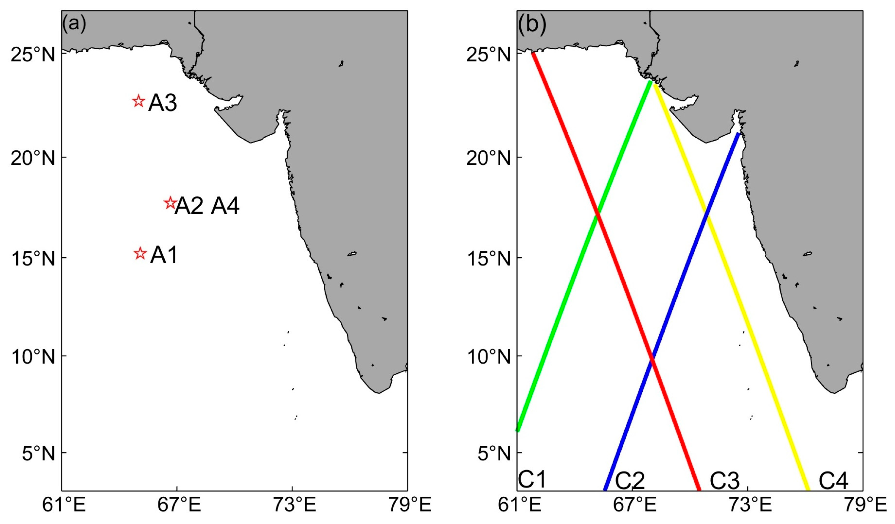
Verification contrast data: Cyclone track information and pressure and maximum sustained wind speed data were obtained from the India Meteorological Department (IMD) website (https://rsmcnewdelhi.imd.gov.in, accessed on 7 November 2025). This study used Argo data from the China Argo real-time data center to obtain the world’s oceans Argo, a scatter dataset (V3.0) (ftp://ftp.argo.org.cn/pub/ARGO/global/, accessed on 7 November 2025). The upper ocean’s vertical resolution can reach 1~2 m, and a detailed analysis of the upper ocean requirements for temperature and salinity changes is also conducted. The locations of the Argo buoys used in this study are shown in Figure 3a. For the SST daily observations from the Operational Sea Surface Temperature and Sea Ice Analysis (OSTIA) system [43,44], OSTIA uses satellite data including those from AMSR-E, AVHRR (GAC + LAC), IASI, SEVIRI, TMI, GOES, SSMIS, and SSM/I sensors together with in situ observations to determine the sea surface temperature. The analysis is produced daily and is provided on a 1/20° regular grid.
To verify the accuracy of the wind and wave simulations, data from the Jason–3 satellite altimeter [45] in the Ku band were used. Jason–3 (https://www.ncei.noaa.gov/data/oceans/jason3/, accessed on 7 November 2025) is a satellite altimeter created by the partnership of the European Organization for the Exploitation of Meteorological Satellites (EUMETSAT) and National Aeronautic and Space Administration (NASA) and is an international cooperative mission in which National Oceanic and Atmospheric Administration (NOAA) is partnered with the Centre National d’Études Spatiales (CNES, French space agency). We select data from four satellite altimeter scans during the TC for wave validation, as shown in Figure 3b. The lines from left to right represent the satellite altimeter trajectories on 7 June, 13 June, 16 June, and 12 June. Their corresponding designations are 341_207, 342_105, 342_168, and 342_066.

3. Results and Discussion

3.1. TC Simulation Validation

The output files of the Weather Research and Forecasting (WRF) model were processed using the NCAR Command Language (Version 6.6.2) [46] (NCL; available at http://dx.doi.org/10.5065/D6WD3XH5, accessed on 7 November 2025). The maximum sustained wind, according to the IMD, is the highest 3 min surface wind occurring within the circulation of the system. These surface winds are observed (or, more often, estimated) at the standard meteorological height of 10 m (33 ft) in an unobstructed exposure (i.e., not blocked by buildings or trees).
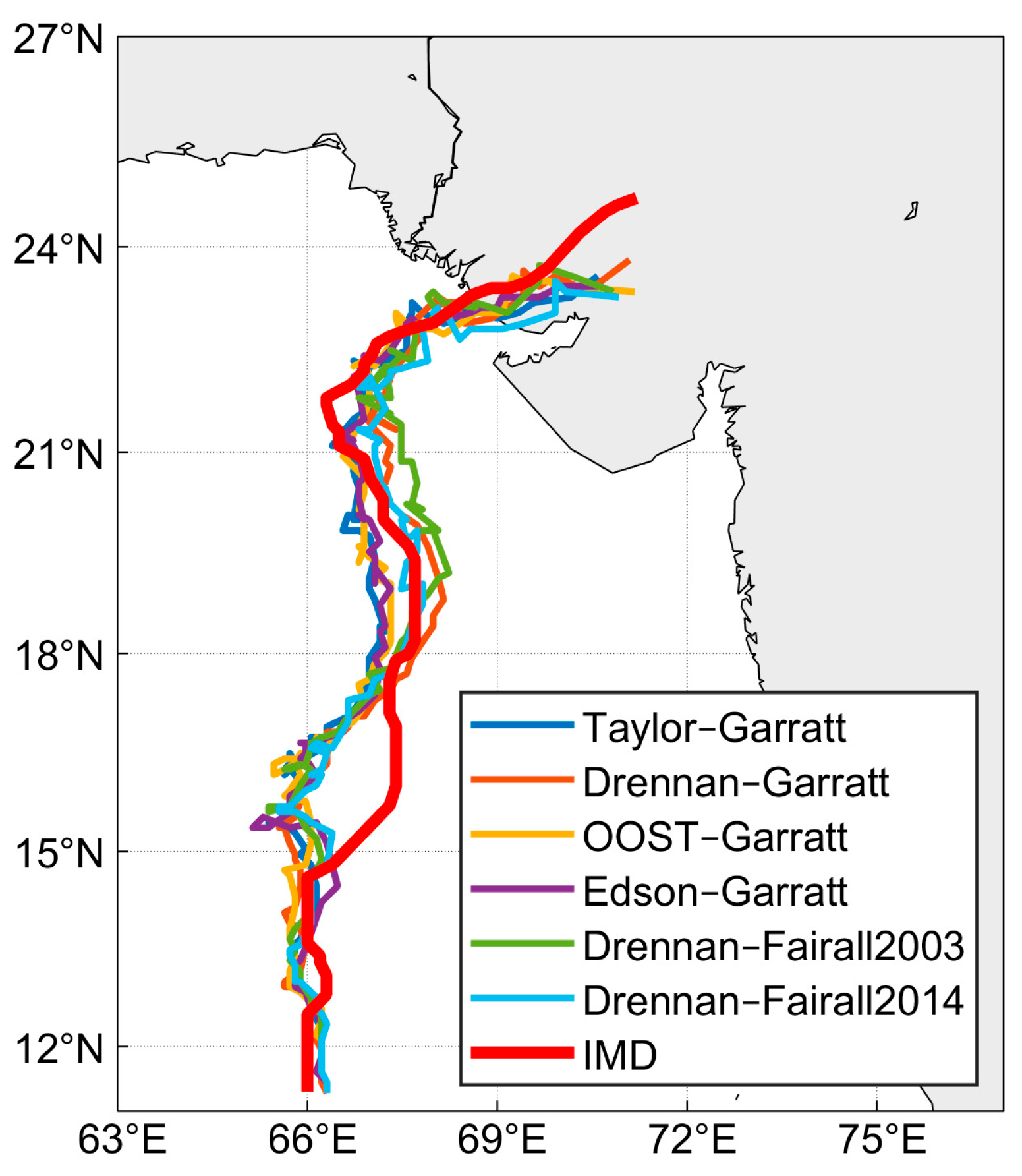
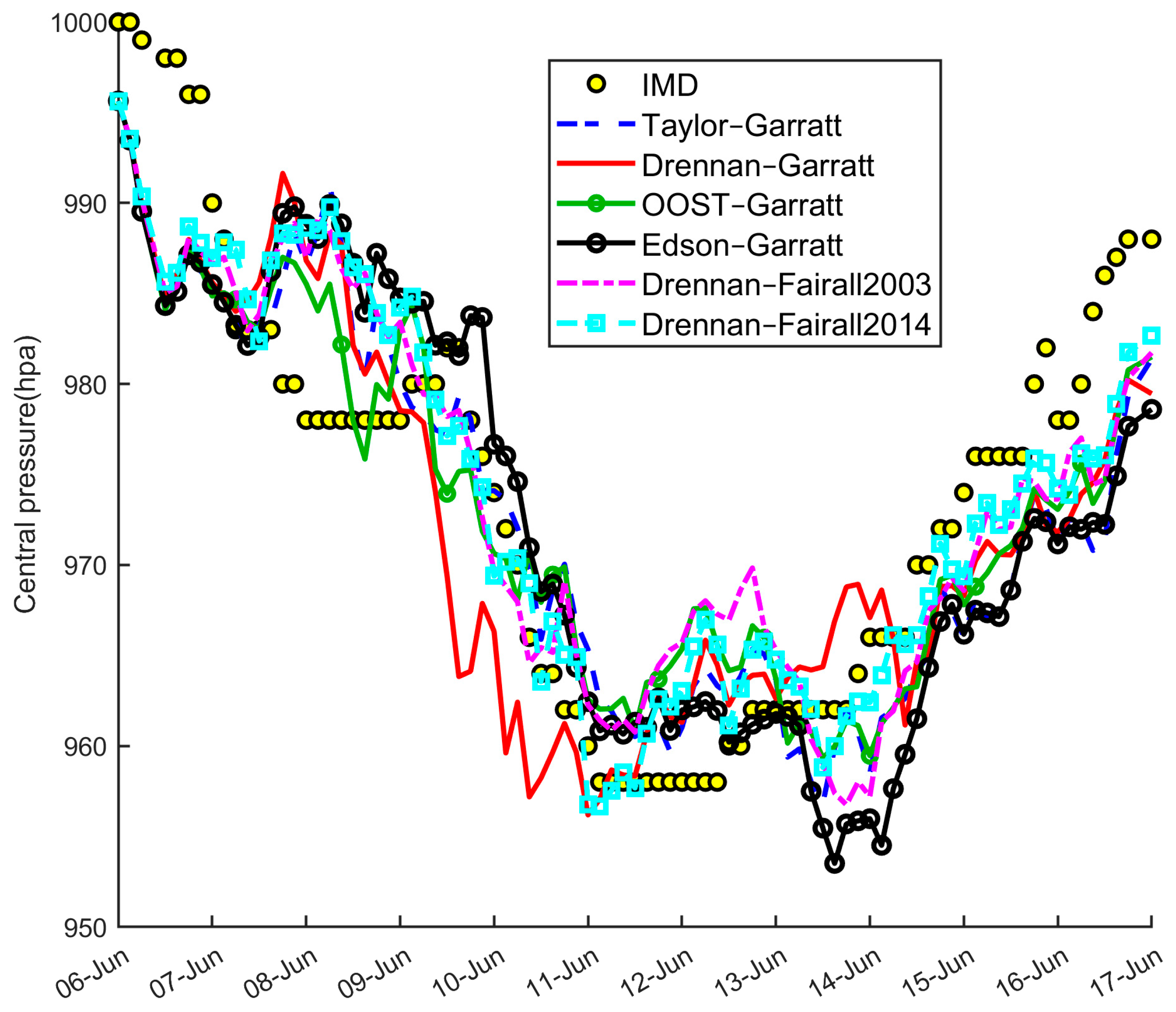
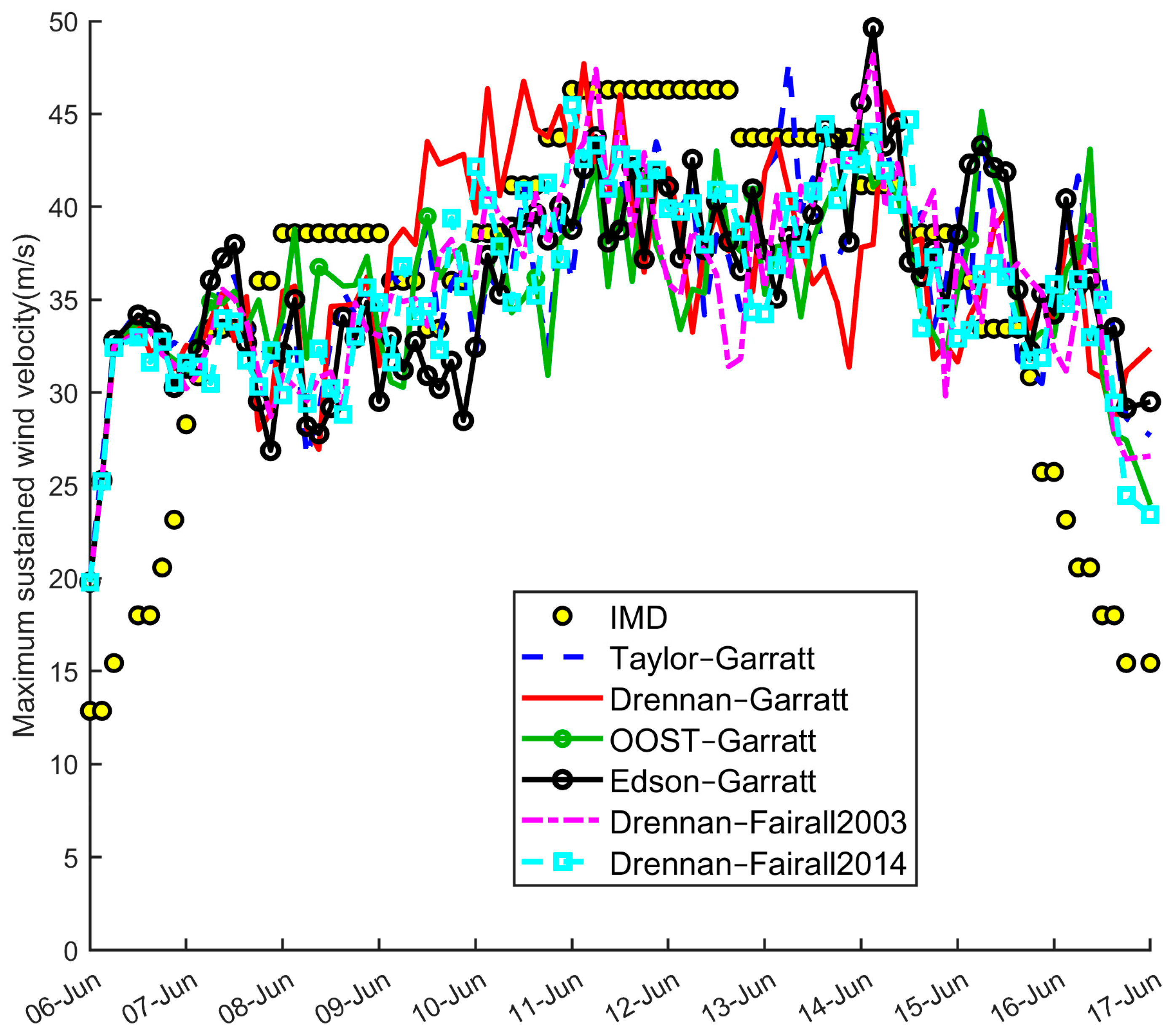
Figure 4 shows the cyclone track experimentally simulated by different models, along with the best track estimates from the IMD. Comparisons of TC central pressure and the maximum sustained wind velocity are also shown in Figure 5 and Figure 6. Detailed comparison data is listed in Table 3. Among the four momentum roughness length schemes evaluated, the Drennan scheme yielded the smallest track error in this simulation, indicating better performance in reproducing the cyclone’s spatial trajectory for this case. However, despite its performance in track simulation, the Drennan scheme did not yield the most accurate results in terms of TC central pressure or the maximum sustained wind speed.
To further investigate the potential of improving the representation of storm intensity, a series of sensitivity experiments incorporating different thermal and moisture roughness length schemes into the Drennan momentum framework was conducted. Among these, the combination of the Drennan momentum scheme with the Fairall2014 thermal and moisture roughness scheme especially improved the simulation of TC central pressure and the maximum sustained wind speed, achieving the smallest errors in both measures across all experiments. Although this combined experiment resulted in a slightly larger track error compared to the standalone Drennan configuration, it still ranked as the second best in terms of TC track error.
Collectively, these findings suggest that while the momentum roughness length plays a critical role in determining the track of TC, the integration of an appropriate thermal and moisture roughness length parameterization is also essential for capturing the thermodynamic processes governing TC intensity.

3.2. Sea Surface Temperature Validation

The sensitivity of SST to the parameterization of roughness length was investigated through a series of experiments. By calculating the RMSE between the model-derived daily mean SST and the OSTIA over the study area (Table 4), it could be found that the six groups of simulation experiments all involve a good simulation of SST, and there is little difference between the experiments. Among the four momentum roughness length schemes evaluated, the Drennan scheme produced the smallest RMSE of SST.
Among different thermal and moisture roughness length schemes, the performance of the schemes can be interpreted through their underlying formulations. The Garratt scheme, which utilizes a more traditional relationship for scalar roughness, established the baseline cold bias. The Fairall2003 scheme, which parameterizes the thermal and moisture roughness length with a slightly different scaling against the roughness Reynolds number, resulted in a marginal mitigation of this bias on average. This modest improvement is attributed to its weaker sensitivity to the roughness Reynolds number, which moderates the turbulent heat exchange under TC conditions.
However, the more recent Fairall2014 scheme, which incorporates an updated formulation that effectively raises the upper limit for the thermal and moisture roughness length, produced the most pronounced cold bias and the largest errors across all forecast lead times. The increased error is attributable to its heightened Reynolds number dependence (–0.72 exponent) and the imposed upper limit of thermal and moisture roughness length. Under high wind and strong turbulence, this formulation enhances thermal and moisture roughness length, thereby leading to greater ocean heat loss.
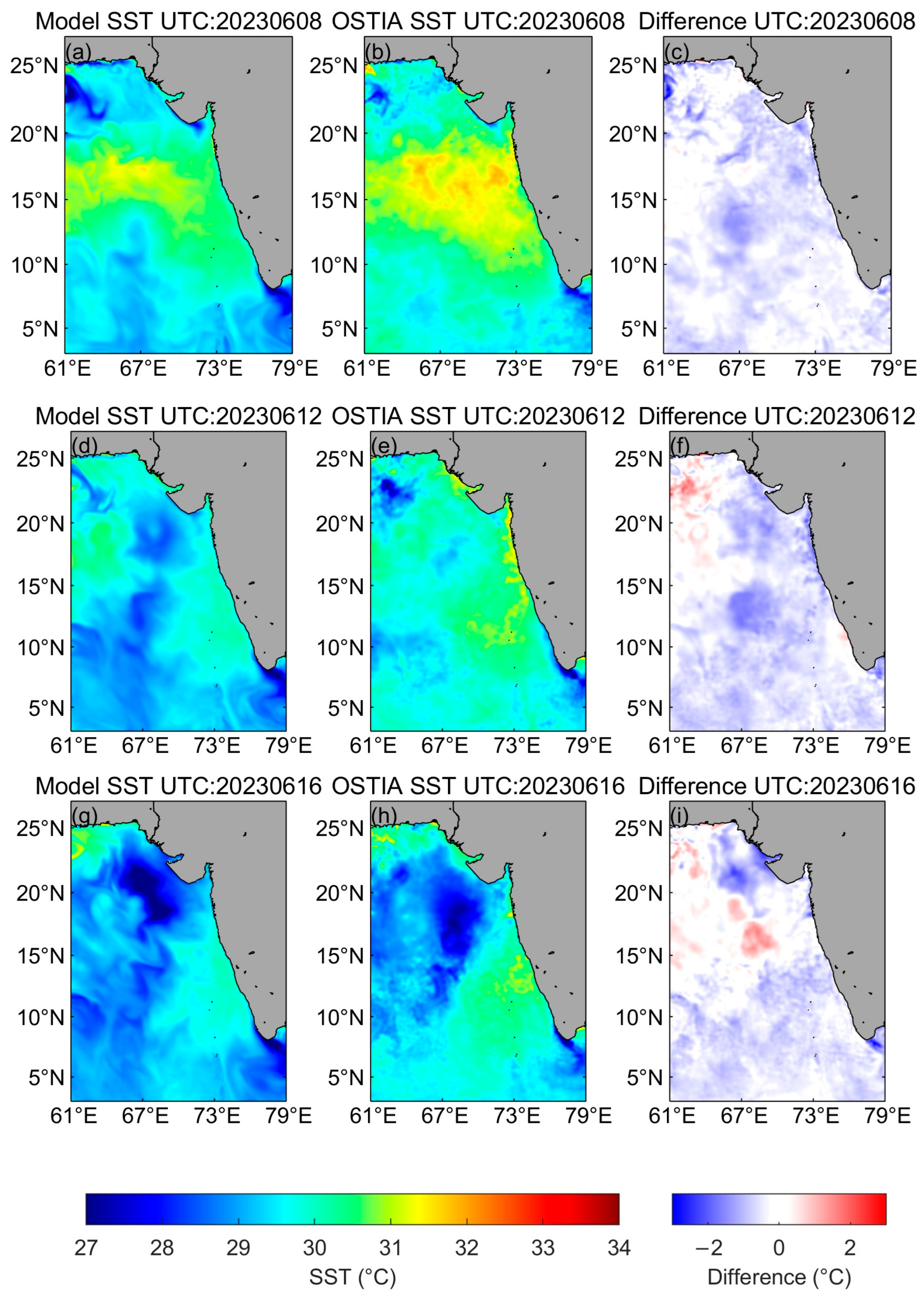
SST exhibits significant cooling under the influence of TC. Figure 7 shows the evolution of SST in the Arabian Sea in the Drennan–Garratt experiment under the impact of TC. As evident in Figure 7a,g, the passage of TC Biparjoy induced significant sea surface cooling around the cyclone center, with a maximum SST decrease exceeding 5 °C in the region of 15–20° N. A pronounced asymmetry is observed in the TC-induced sea surface temperature cooling, characterized by a more substantial decrease to the right of the storm’s path. Figure 7a,g reveal this disparity, with the maximum cooling surpassing about 5 °C on the right side versus merely 3 °C on the left.

3.3. Argo Validation

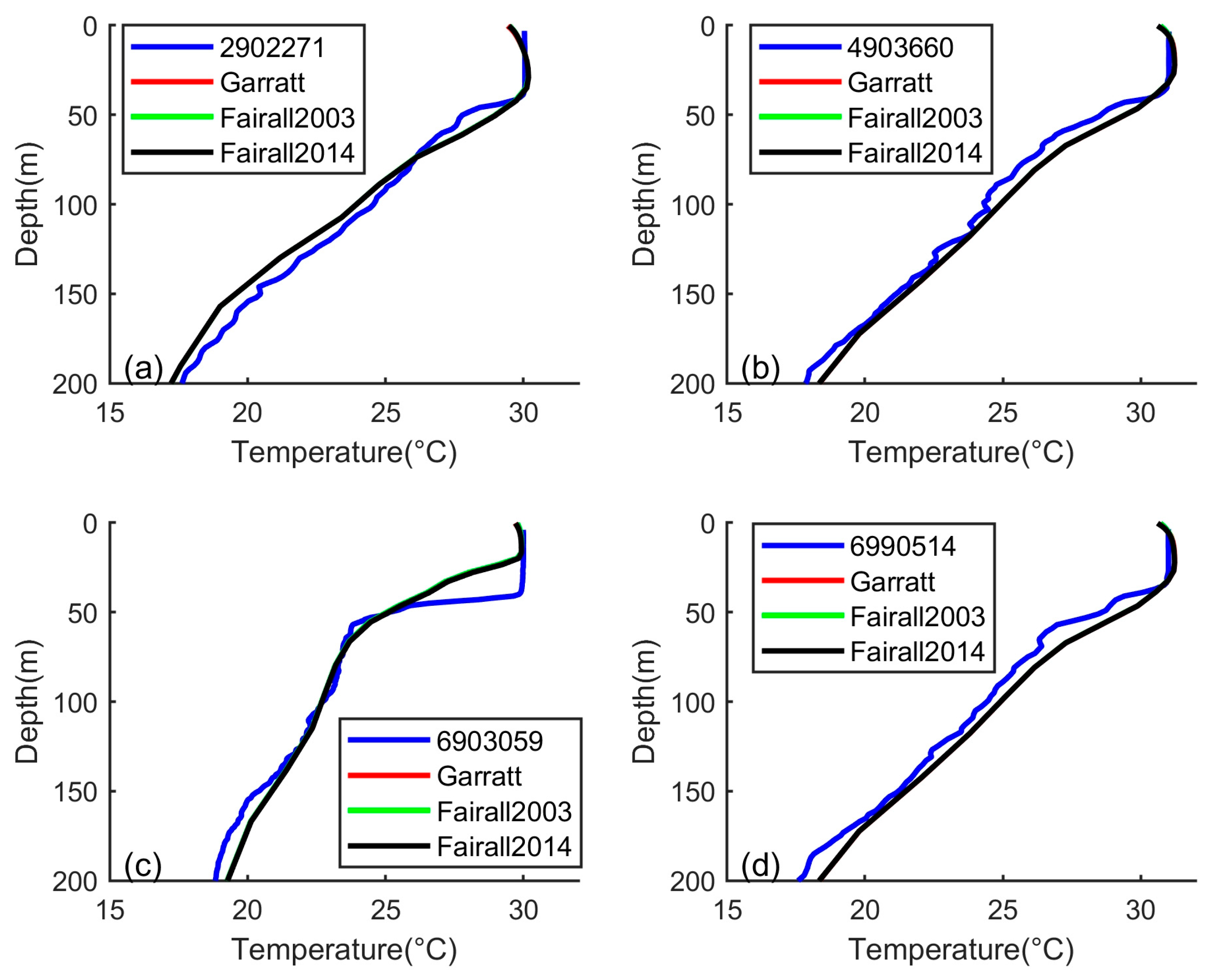
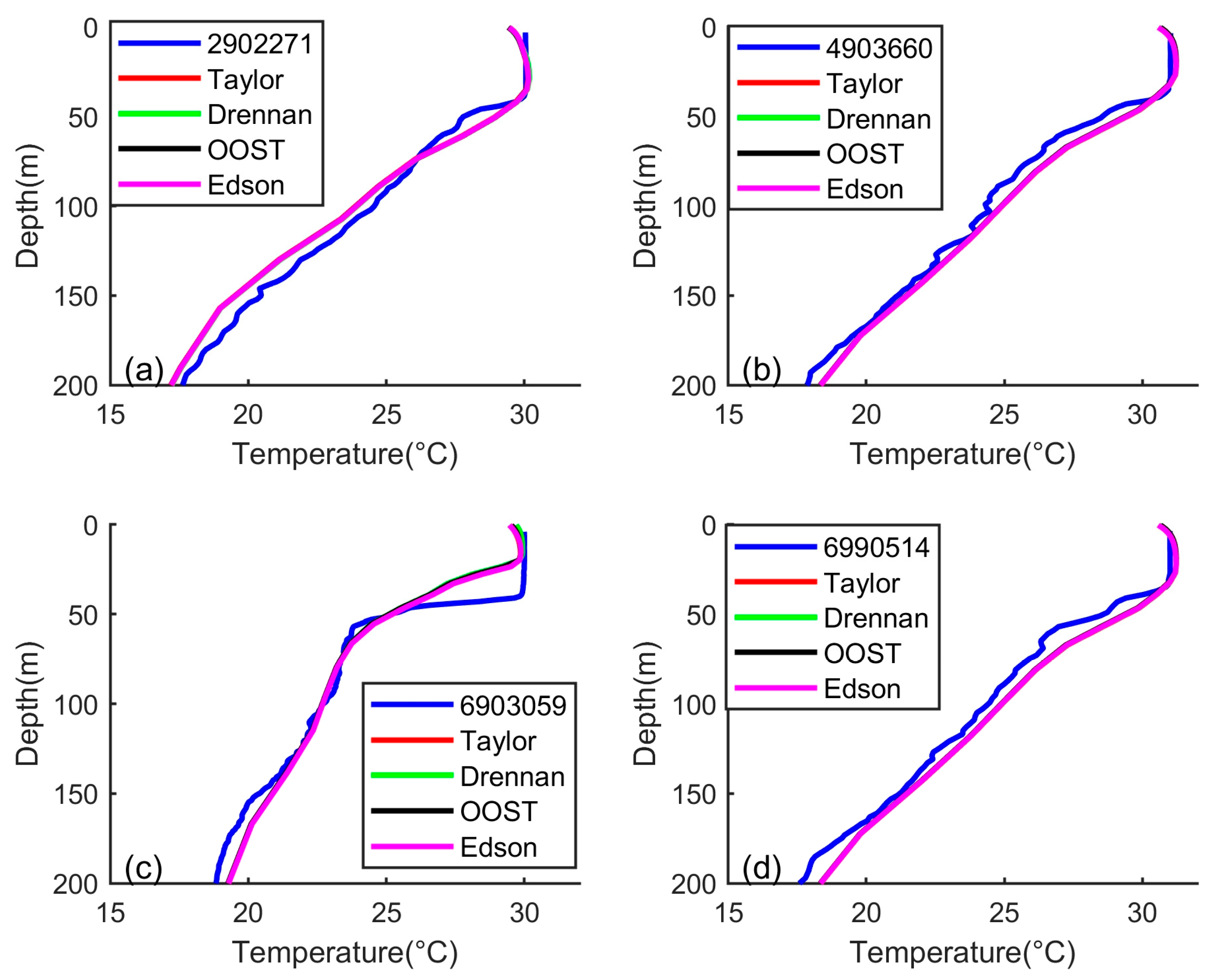
Four buoys were selected to compare temperature profiles, three of which were close to the path of the TC, namely 4903660_006 (91.2025 km), 6903059_364 (166.1553 km), and 6990514_006 (91.357 km). Overall, differences between the model simulations and Argo observations were predominantly confined to the upper ocean (0~200 m). Furthermore, the results from the six sensitivity experiments were generally consistent, exhibiting only minor differences in the surface layer. Figure 8 and Figure 9 show the contrast curve of temperature between the model and Argo profile data. The MAE and Surface Layer Temperature Error (SLTE) are also indicated in Table 5.
Based on the comparative analysis against Argo profile data, the sensitivity experiments reveal a systematic cold bias in the simulated upper ocean thermal structure, a finding consistent with the previously found SST cold bias. The performance of the four momentum roughness length schemes (all paired with the Garratt scheme) varied. The Drennan and OOST schemes generally yielded the most favorable combinations of the MAE and SLTE. Notably, the Edson scheme consistently resulted in the largest cold biases near the TC center, indicating that under high-wind-speed conditions, its adaptability is inferior to the scheme based on wave parameters.
The sensitivity to thermal and moisture roughness length parameterization was even more pronounced. When keeping the momentum scheme constant (Drennan), the Fairall2003 parameterization significantly mitigated the cool bias, producing the smallest SLTE across all periods. The simulated behavior aligns with the earlier SST analysis, confirming its skill in representing the surface layer’s heat exchange. Conversely, the newer Fairall2014 scheme, which imposes a higher upper limit on the thermal and moisture roughness length, intensified turbulent heat loss and consistently resulted in a larger cold bias than its 2003 version. The results confirm that the updated constraints in the Fairall2014 scheme are less suitable for this model case.
According to the above, this analysis identifies the optimal model configuration for ocean thermal feedback as the combination of the Drennan momentum roughness length scheme with the Fairall2003 thermal and moisture and roughness length scheme. This configuration demonstrably minimizes both overall error and the systematic cold bias in the upper ocean, leading to the most robust representation of thermal feedback.

3.4. Jason3 Validation

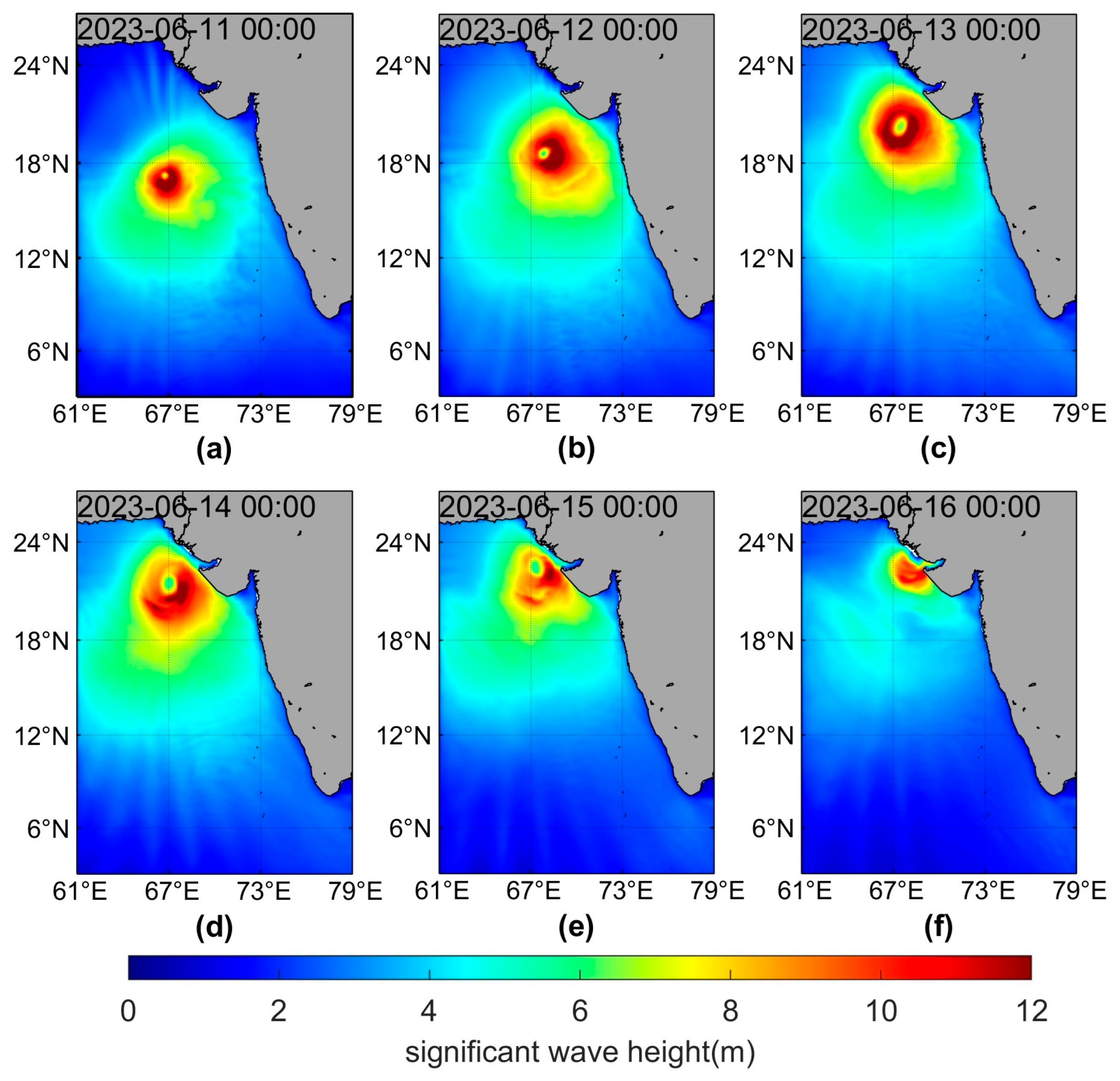
Following TC formation, strong winds transfer substantial energy to the sea surface, driving the generation of large waves. Figure 10 illustrates the characteristics of SWH simulated by the COAWST coupled model from June 11 to June 16. TCs produce energetic waves that significantly disrupt oceanic states. In contrast, regions outside the TC’s influence exhibit significantly lower sea states, with SWH consistently below 1.5 m.
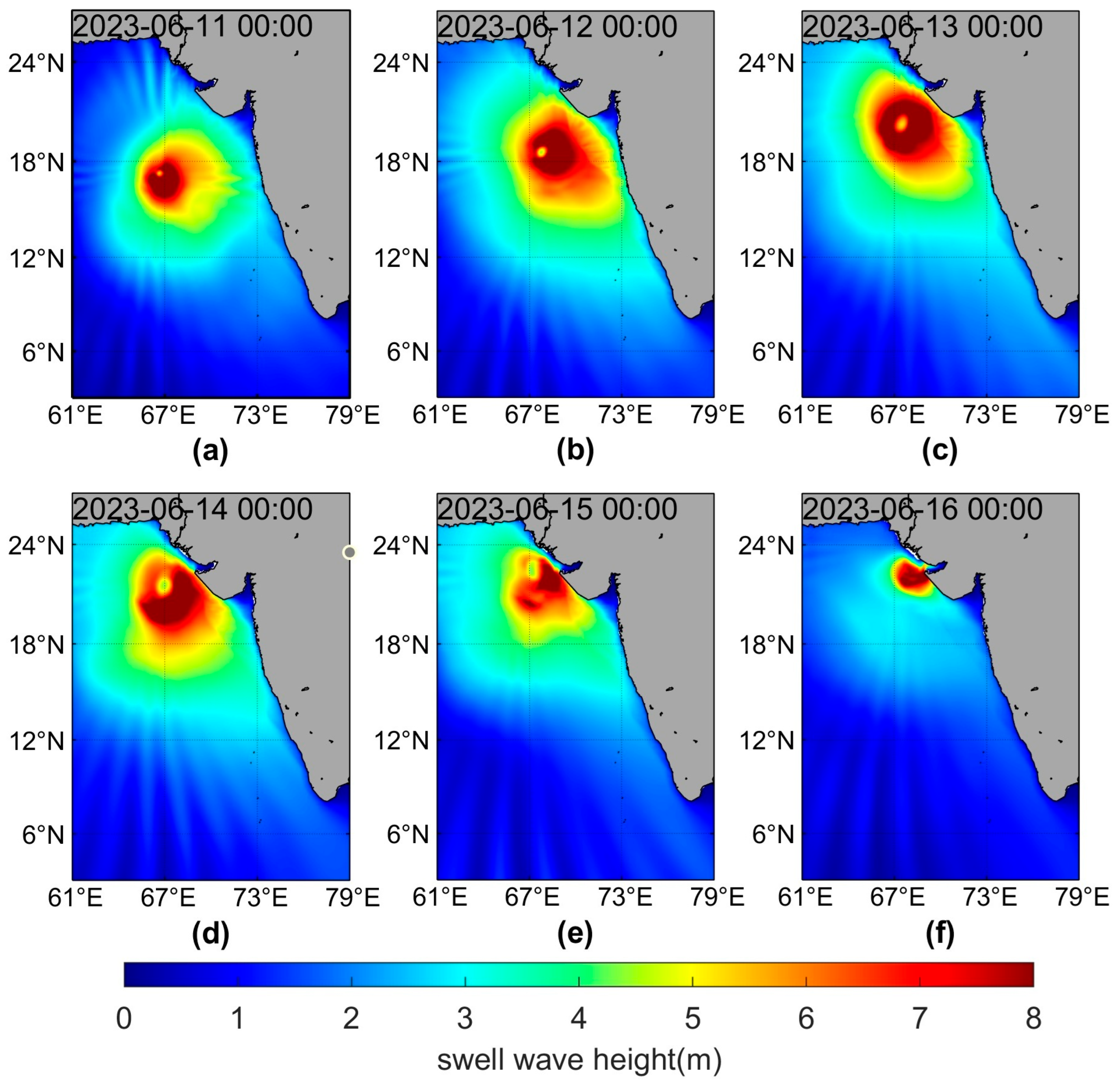
In the high-wind regions of a cyclone, wind waves receive substantial energy input, resulting in high energy density and group velocity. These waves propagate outward into adjacent low-wind zones, evolving into swells. In the outer regions of the typhoon, these remotely generated swell waves mix with local wind waves and typically dominate the combined wave field.
However, the spatial distribution of this swell field can be significantly influenced by numerical discretization effects, particularly the garden sprinkler effect (GSE), as identified in the wave model. The GSE arises from an incompatibility in discrete model resolutions, where coarse directional spectral resolution causes the swell field, which should be continuous, to disintegrate into discrete, unrealistic bands during spatial propagation [47]. This results in an unnatural redistribution of wave energy in the model domain, a phenomenon which is more evident in the swell wave distribution depicted in Figure 11. Superimposed on this numerical artifact is the physical process of wave diffraction, which occurs when these long-period swells interact with seabed topography, leading to a further physical redistribution of wave energy.
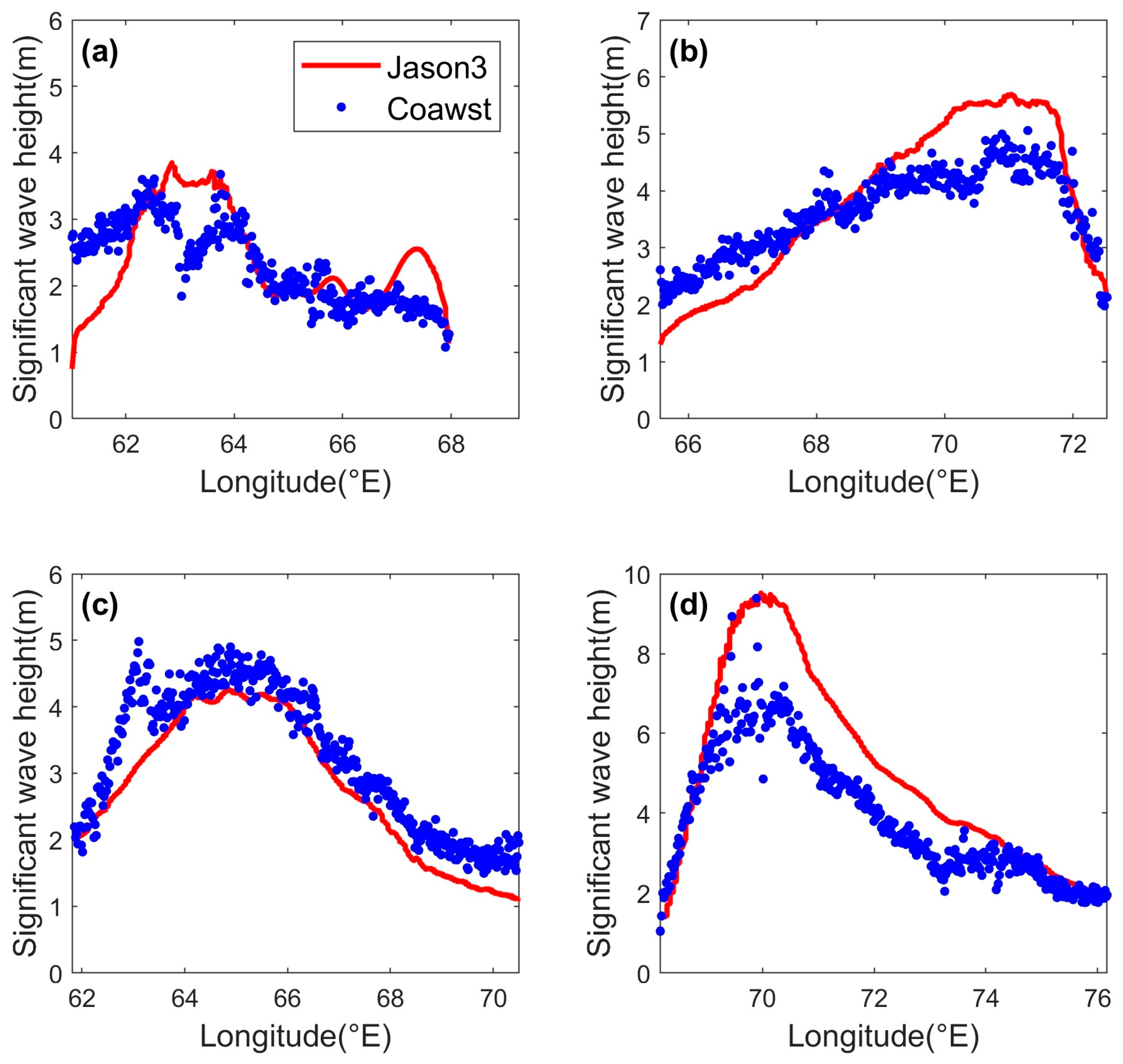
As shown in Figure 12 and Table 6, the evaluation of SWH simulations against Jason3 data reveals certain variability in model performance across different periods and parameterization schemes. No single scheme consistently performs better than all others across the four evaluation periods (341_207, 342_066, 342_105, 342_168), as measured by both the MAE and MAPE. This indicates a strong dependence of model skill on the specific oceanic conditions being simulated. The Drennan–Garratt and Drennan–Fairall2014 configurations exhibit the largest errors during period 342_066 (MAE > 1, MAPE > 25%), suggesting a potential deficiency in these schemes under the high-wave conditions likely present during this time. In contrast, the Edson–Garratt scheme performs notably well for this same period, achieving the lowest MAE (0.7101) and MAPE (16.19%). However, during other periods, the Drennan scheme shows a significant improvement, delivering the lower MAE. The variability in performance indicates that while it may fail during extreme events, its formulation is effective under more moderate conditions. The Edson–Garratt and Drennan–Fairall2003 schemes also demonstrate strong and consistent performance in these periods, with low errors.

3.5. Analysis of Surface Roughness Lengths and Exchange Coefficients

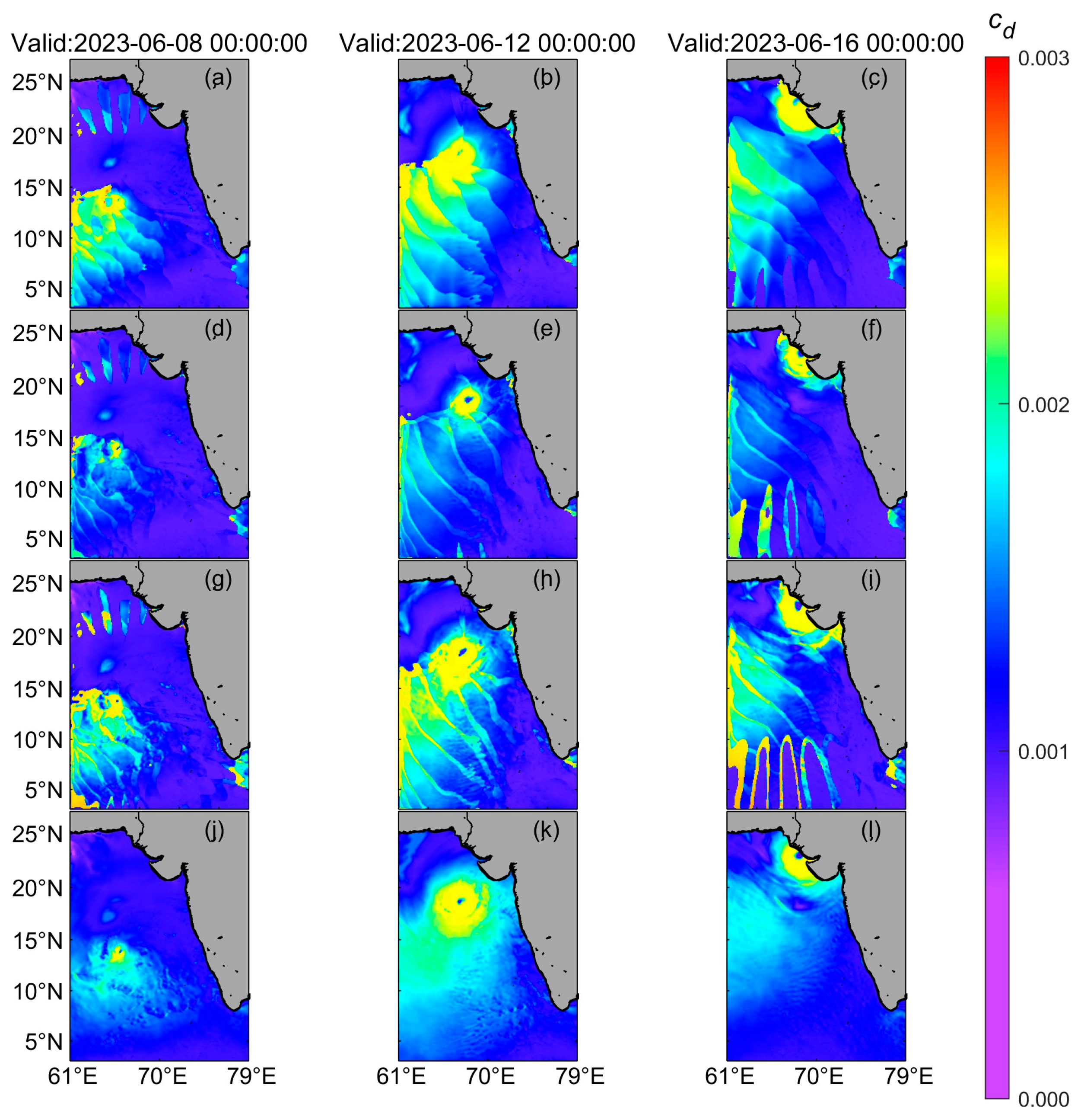
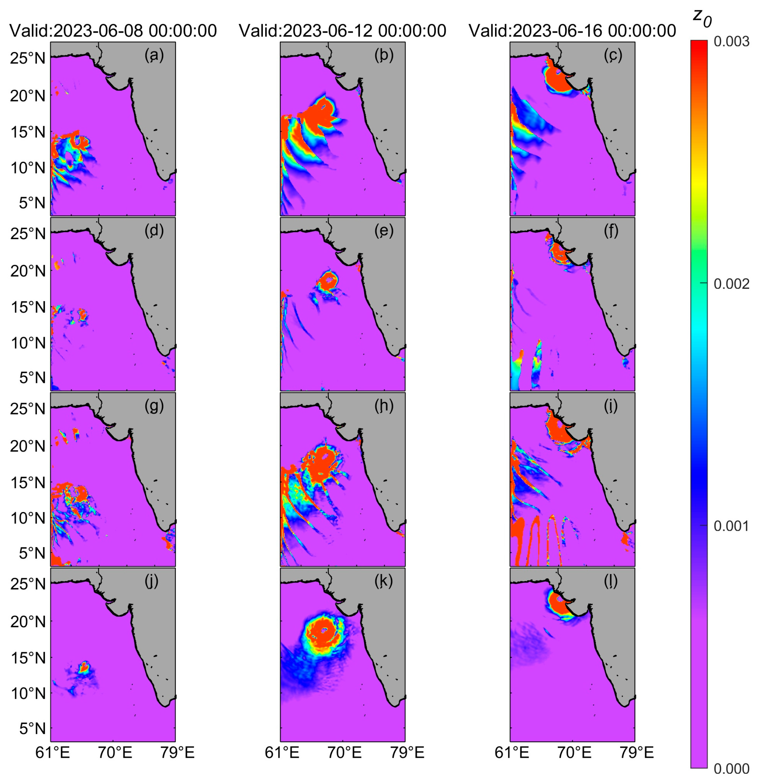
The momentum roughness lengths and drag coefficients of four parameterizations of Taylor, Drennan, Oost, and Edson for 3 days from days 08 to 16 with an interval of 4 days are plotted (Figure 13 and Figure 14). All four parameterizations consistently show an increase in both momentum roughness length and drag coefficient with rising wind speed. The increasing trend continues until the Davis limiter is reached. The saturation characteristics of the drag coefficient obtained in our simulations align with existing theoretical understanding, which attributes this behavior to physical processes such as flow separation and wave breaking under extreme wind speeds. Although the current model does not explicitly include a parameterization for sea spray effects, the simulation results correspond effectively with this theoretical mechanism.
The simulated momentum roughness length exhibits clear scale differences across the parameterization schemes. The Drennan scheme produces the lowest values, followed by that of Edson, while the Taylor and Yelland and Oost schemes yield similar magnitudes. The resulting relationship can be summarized as follows: Drennan < Edson < Taylor ≈ Oost. This ranking in momentum roughness length aligns physically with the TC intensity performance analyzed in Section 3.1. A lower momentum roughness length under the Drennan scheme reduces momentum transfer from the atmosphere to the ocean, which subsequently dampens ocean surface mixing and improves the realism of simulated sea surface cooling and upper ocean thermal structure. A more accurate ocean state, in turn, enhances energy feedback to the atmospheric model, ultimately contributing to the more accurate track and intensity forecasts achieved with the Drennan parameterization.
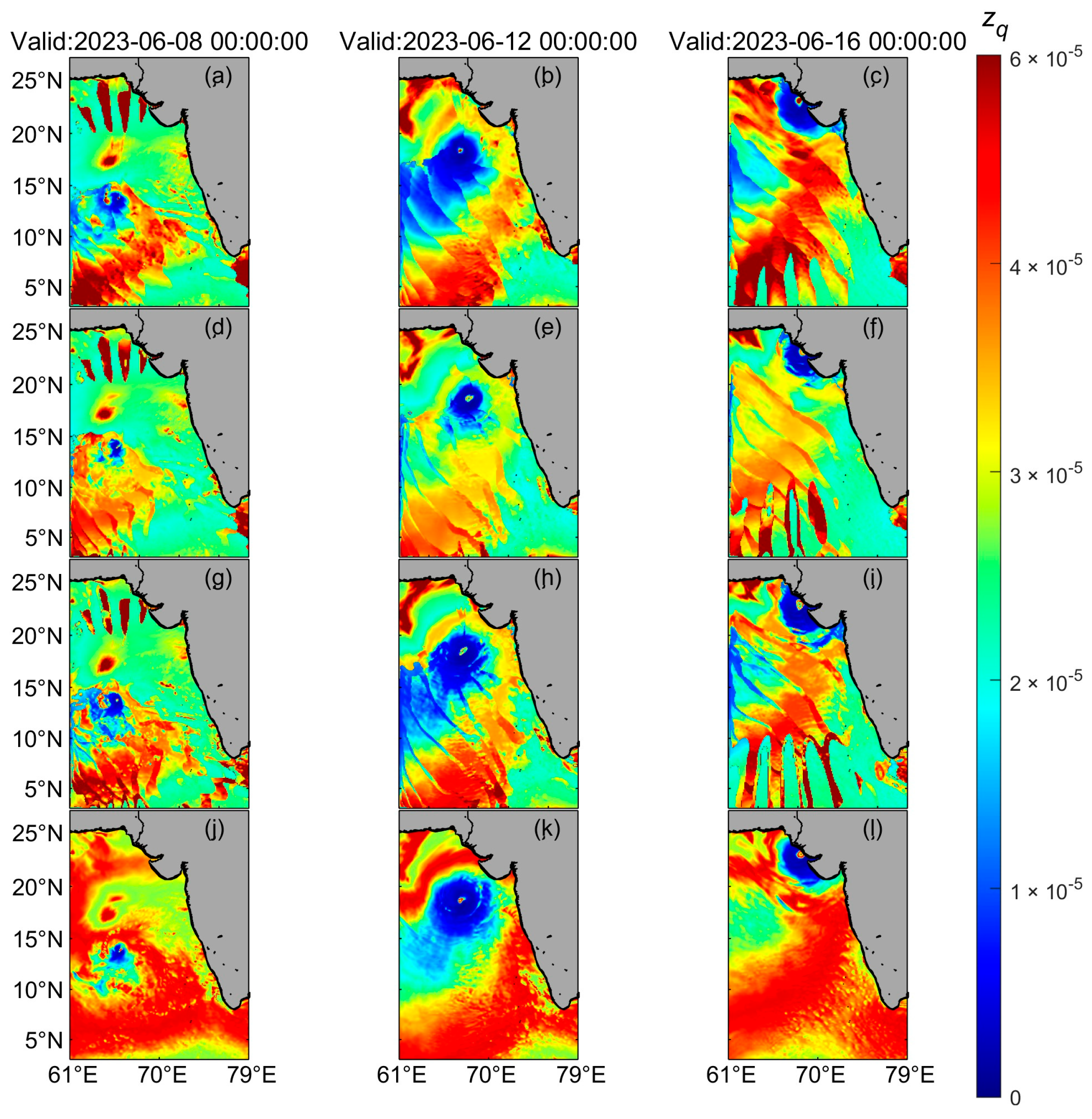
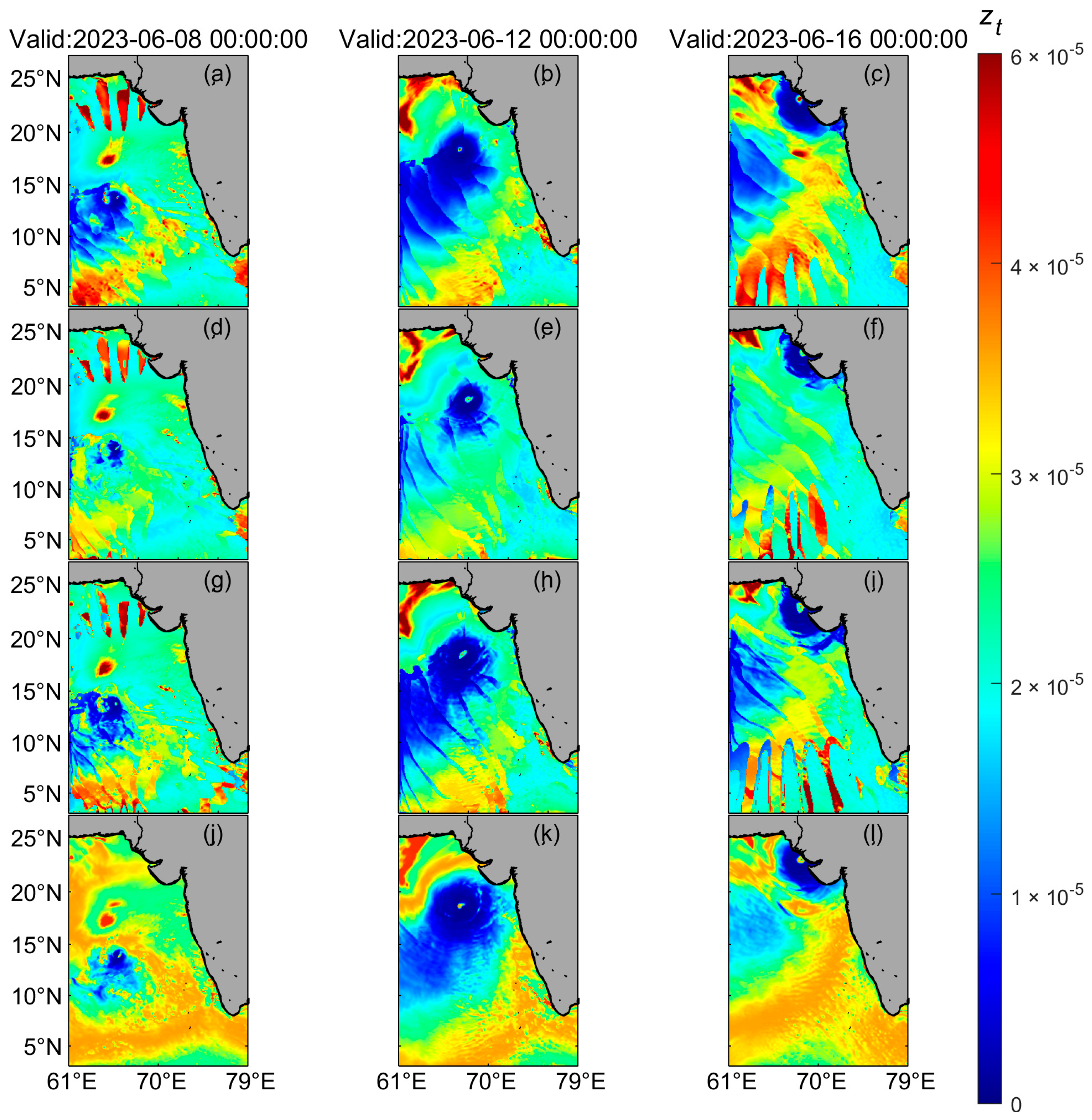
All four sets of experiments consistently reveal a common spatial pattern in the thermal and moisture roughness lengths (Figure 15, Figure 16 and Figure 17): they reach their minimum in the typhoon’s central region and their maximum in the convective active bands outside the TC center. Such a spatial distribution carries significant physical implications: the lower roughness in the TC center acts to suppress local sensible and latent heat exchange (i.e., enthalpy flux). Given that the central region is one of the strongest areas for ocean upwelling and mixing induced by the storm, excessively high heat fluxes here would drastically intensify sea surface cooling, creating a potent cold pool that could sever the storm’s energy supply.
Furthermore, in regions remote from the typhoon center, for example, within 5–10° N, band-like or strip-like distributions of roughness lengths are evident. This pattern is linked to the GSE mentioned in Section 3.4. The combined effect of numerically induced (GSE) and physically based (diffraction) wave field heterogeneity is subsequently conveyed through wave-dependent roughness length parameterization schemes, thereby directly modulating sea surface roughness and ultimately imprinting a corresponding band-like spatial pattern onto the air–sea momentum exchange efficiency, i.e., the drag coefficient. This finding underscores that accurately assessing the remote influence of TCs through wave parameter-dependent roughness parameterizations requires not only considering physical swell–topography interactions but also being mindful of discretization-induced phenomena such as the GSE, which arises from the algorithmic representation of continuous wave propagation in discrete models.
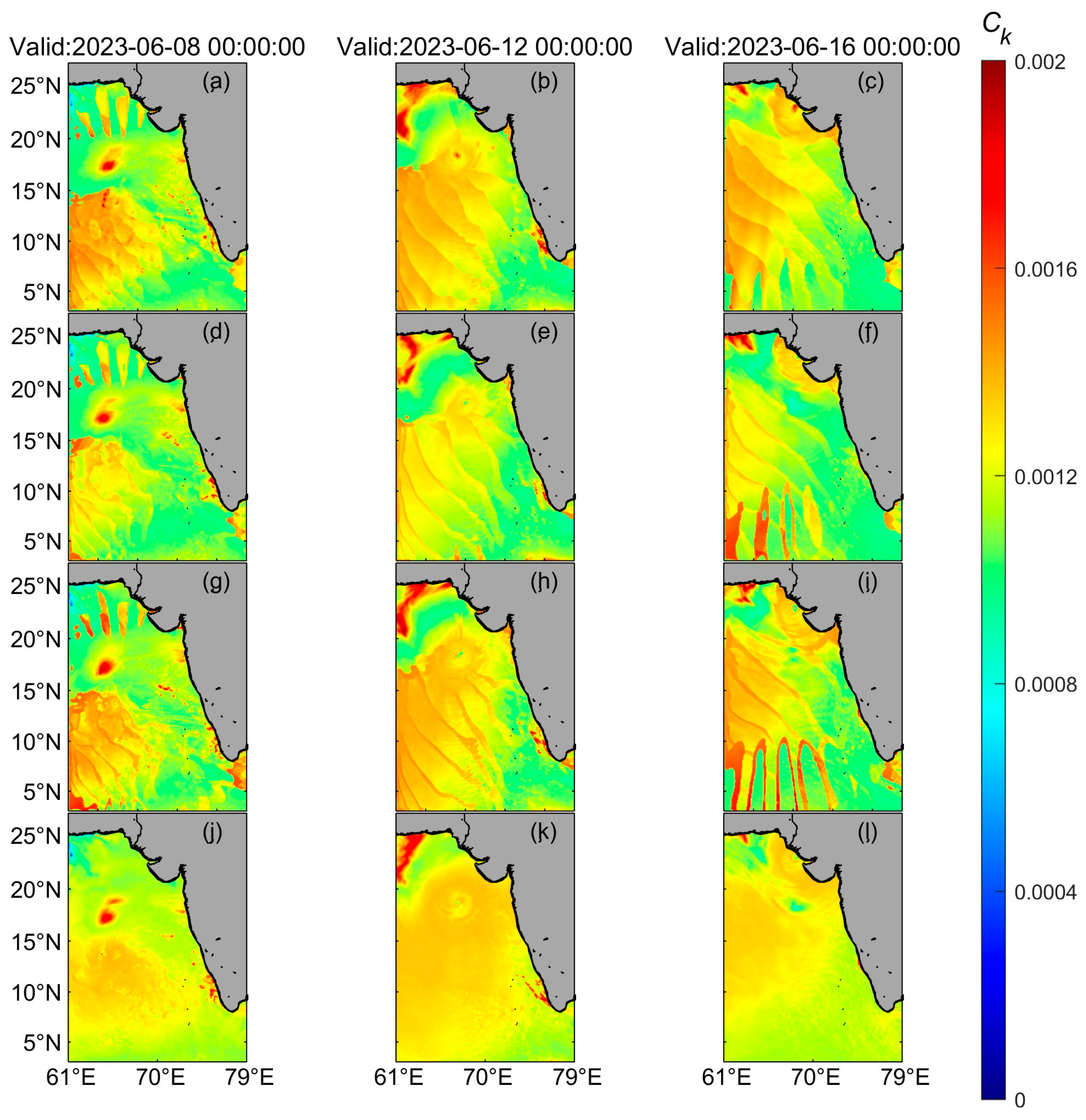
Beyond this commonality, the Drennan scheme exhibits a critical distinction: it produces the largest thermal and moisture roughness lengths, particularly within the TC center, yet corresponds to the smallest enthalpy exchange coefficient (Ck). The relatively smaller thermal and moisture roughness lengths directly curb excessive heat exchange within the TC center. These constraints effectively limit excessive heat exchange via a smaller effective exchange coefficient. The suppression of the heat flux significantly weakens the ocean’s self-cooling negative feedback, effectively mitigating excessive sea surface cold bias and thereby maintaining the positive ocean heat content anomaly crucial for sustained TC intensification.
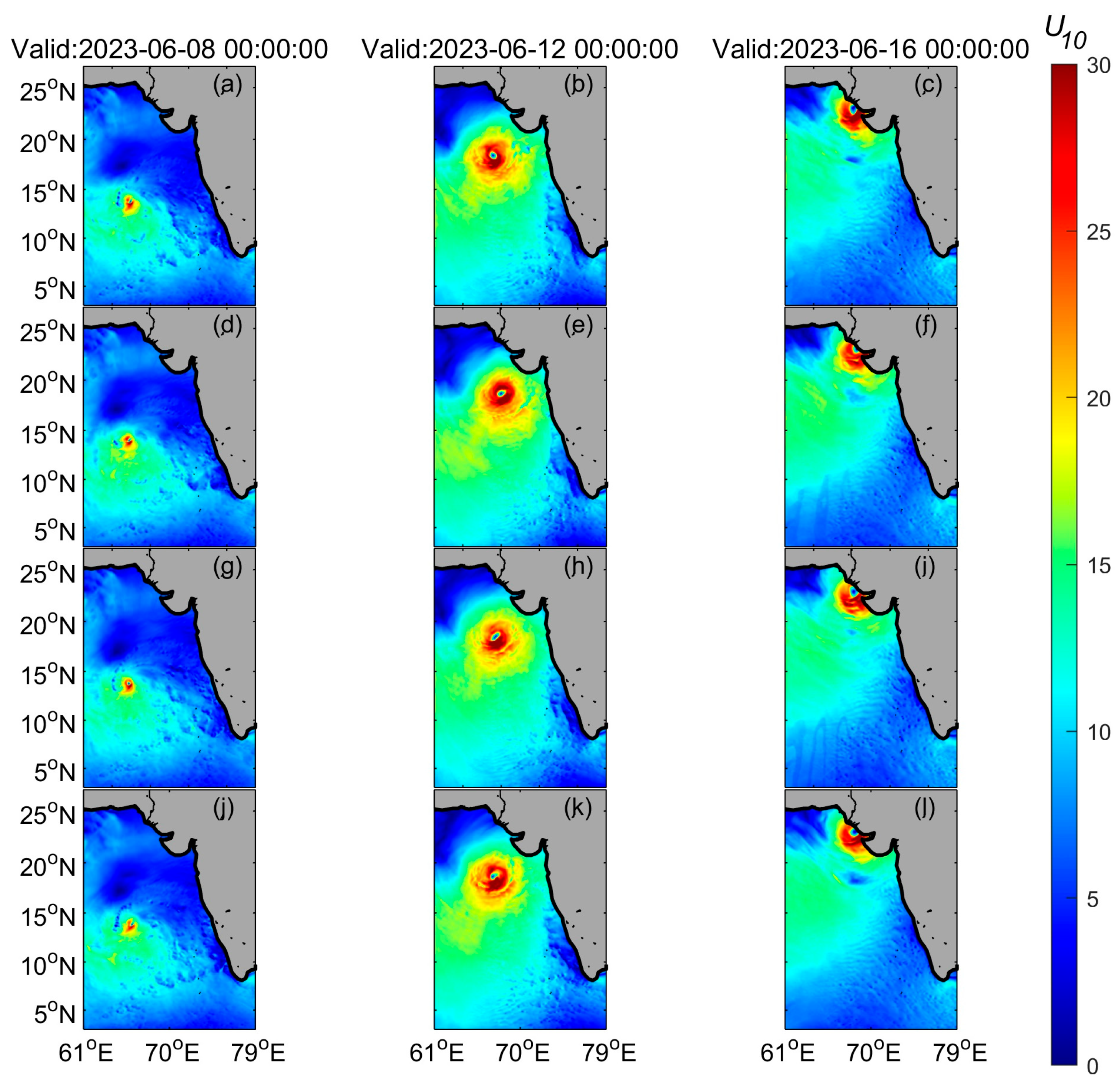
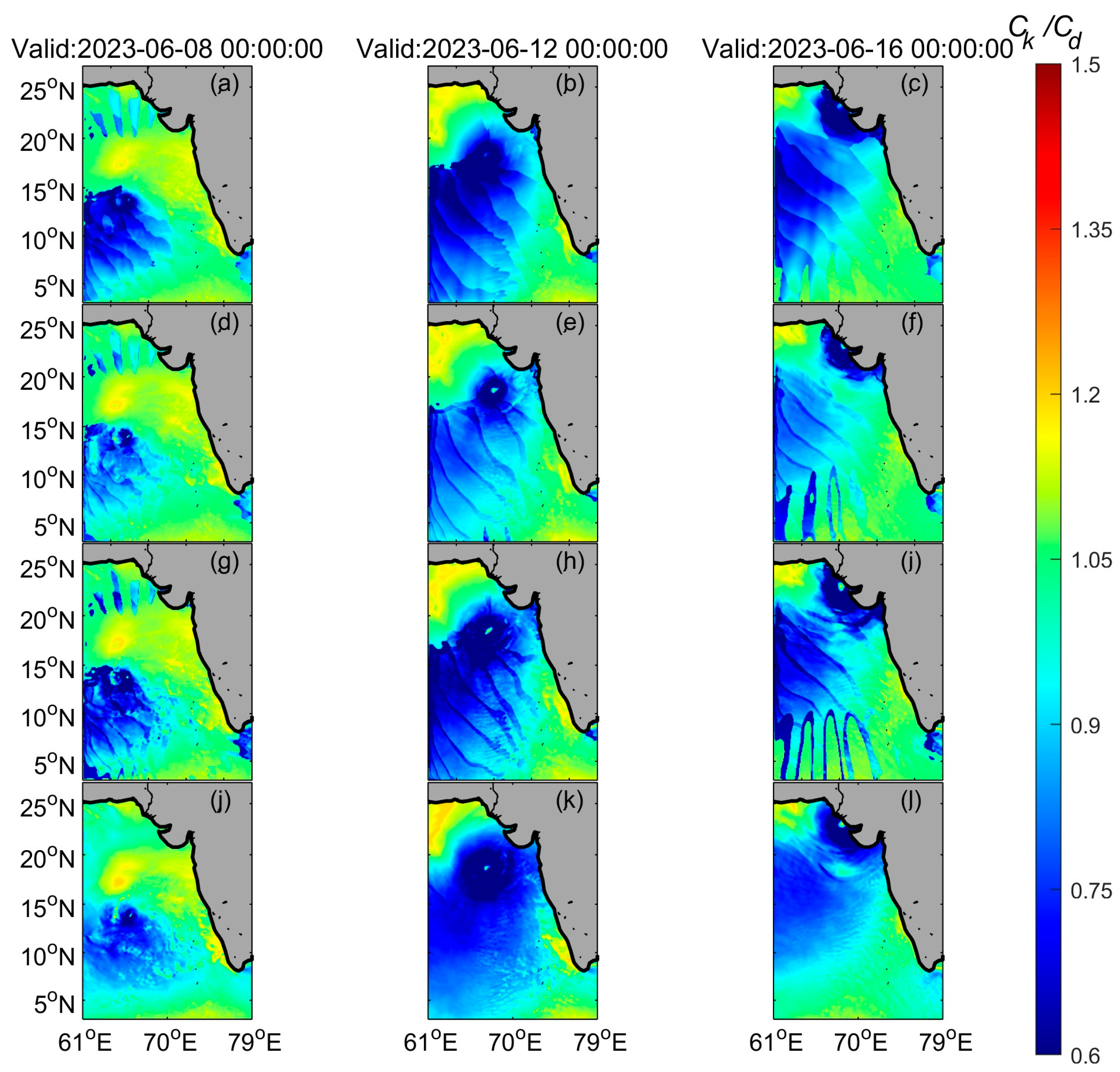
To further elucidate the role of surface exchange coefficients under high-wind conditions, and in direct response to reviewer suggestions, we supplemented the analysis in this section with two additional diagnostics: the spatial distribution of the Ck/Cd ratio (Figure 18) and the corresponding 10 m wind speed (Figure 19). These results show that the Ck/Cd ratio near the radius of maximum wind (RMW) averages approximately 0.7, which is slightly lower than the 0.75 lower bound proposed by Emanuel [7]. This value is nevertheless physically plausible within our coupled modeling framework. As highlighted by Bryan [10], the simulated ratio Ck/Cd and its influence on storm intensity are sensitive to the representation of horizontal turbulent diffusion (lh). Emanuel’s conclusion was based on simulations employing relatively strong horizontal diffusion (lh ≈ 3000 m) and a low sea surface temperature (26 °C). In contrast, the present study uses the fully coupled COAWST system, in which the momentum roughness length (and hence the surface momentum exchange) is dynamically updated using wave information from SWAN. This wave-dependent representation of drag likely yields a boundary-layer structure and energy-partitioning behavior that differ from those in simpler prescribed-roughness models, thereby supporting a Ck/Cd ratio around 0.7 under the high-wind, fully coupled conditions simulated for Cyclone Biparjoy. The inclusion of these diagnostics provides a more observationally grounded perspective on enthalpy-to-momentum exchange efficiency and strengthens the attribution of surface flux effects in our sensitivity experiments.
In conclusion, the relative advantage of the Drennan scheme in this study lies in its ability to optimize the energy cycle of the typhoon system through a physically self-consistent and spatially coherent roughness distribution. Rather than simply delivering the largest or smallest fluxes, it precisely modulates the spatiotemporal pattern of energy exchange while also weakening ocean negative feedback and optimizing the internal energy allocation pathway, ultimately leading to improved intensity forecasts.

3.6. Result of Simulated Fluxes

In comparing the fluxes from different parameterization schemes, we focus on their direct impact. Since the simulated SST fields showed limited sensitivity to the roughness length choices (see Section 3.2 and Section 3.3), the contribution from SST-coupled feedbacks to the flux differences is assumed to be secondary. Thus, the flux comparisons in Section 3.6.1 and Section 3.6.2 largely reflect the immediate effects of the parameterizations on air–sea exchange.

3.6.1. Momentum Flux

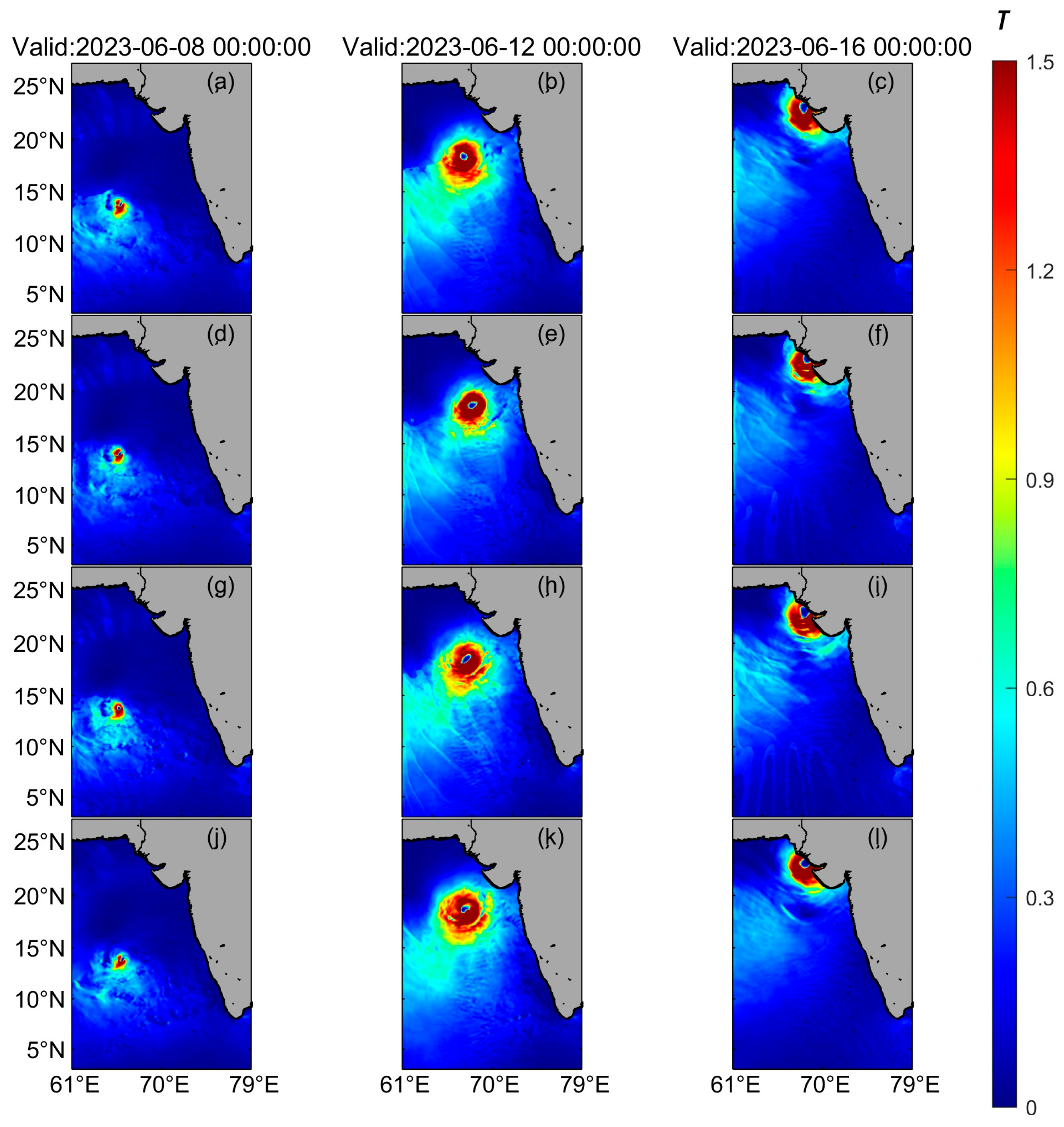
As a direct manifestation of momentum roughness parameterization, the spatial distributions of momentum flux across the four experiments are broadly similar, as illustrated in Figure 20. The maximum values are consistently concentrated in convective regions a certain distance from the TC center. While the cyclone core concentrates immense energy, it is primarily through organized convective ascent and latent heat release that this energy is dissipated. The turbulent process responsible for the downward transfer of momentum is not the strongest in this central region. Consequently, despite harboring the highest wind speeds, the cyclone core does not exhibit the peak momentum flux.
Notably, the momentum flux simulated by the Drennan scheme is weaker near the typhoon center compared to the other three experiments. The simulated behavior aligns with the theoretical expectation: the lower roughness length specified in the Drennan scheme reduces the momentum exchange at the air–sea interface (i.e., momentum flux). The resultant reduction in momentum exchange, in turn, diminishes the dissipation efficiency of kinetic energy in the surface layer, allowing more energy to remain within the mean flow and ultimately resulting in a higher maximum sustained wind speed. The maximum sustained wind speeds on the 12th provide excellent validation for this physical mechanism: Drennan (42.04 m/s) > Taylor (41.43 m/s) ≈ Edson (41.08 m/s) >> Oost (36.19 m/s). This ranking of wind speeds is entirely consistent with the intensity differences predicted by the momentum roughness lengths of the varying parameterizations.

3.6.2. Sensible and Latent Heat Fluxes

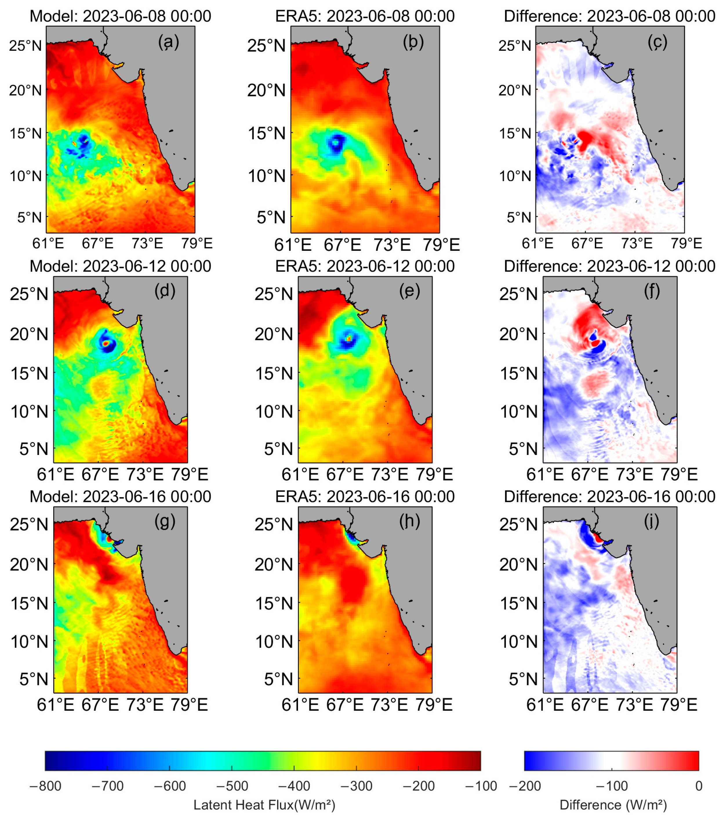
Heat flux, comprising latent and sensible components, plays a critical role in air–sea heat exchange during TCs. Figure 21 shows the spatial distribution of the surface latent heat flux obtained by the coupled COAWST model at different times in the Arabian Sea during TC Biparjoy. It can be seen from the figure that the extremum position of surface latent heat flux occurs near the center of the TC and can reach about −700 W/m2. In the nearshore region, the surface latent heat flux when the TC is landing can exceed −800 W/m2.
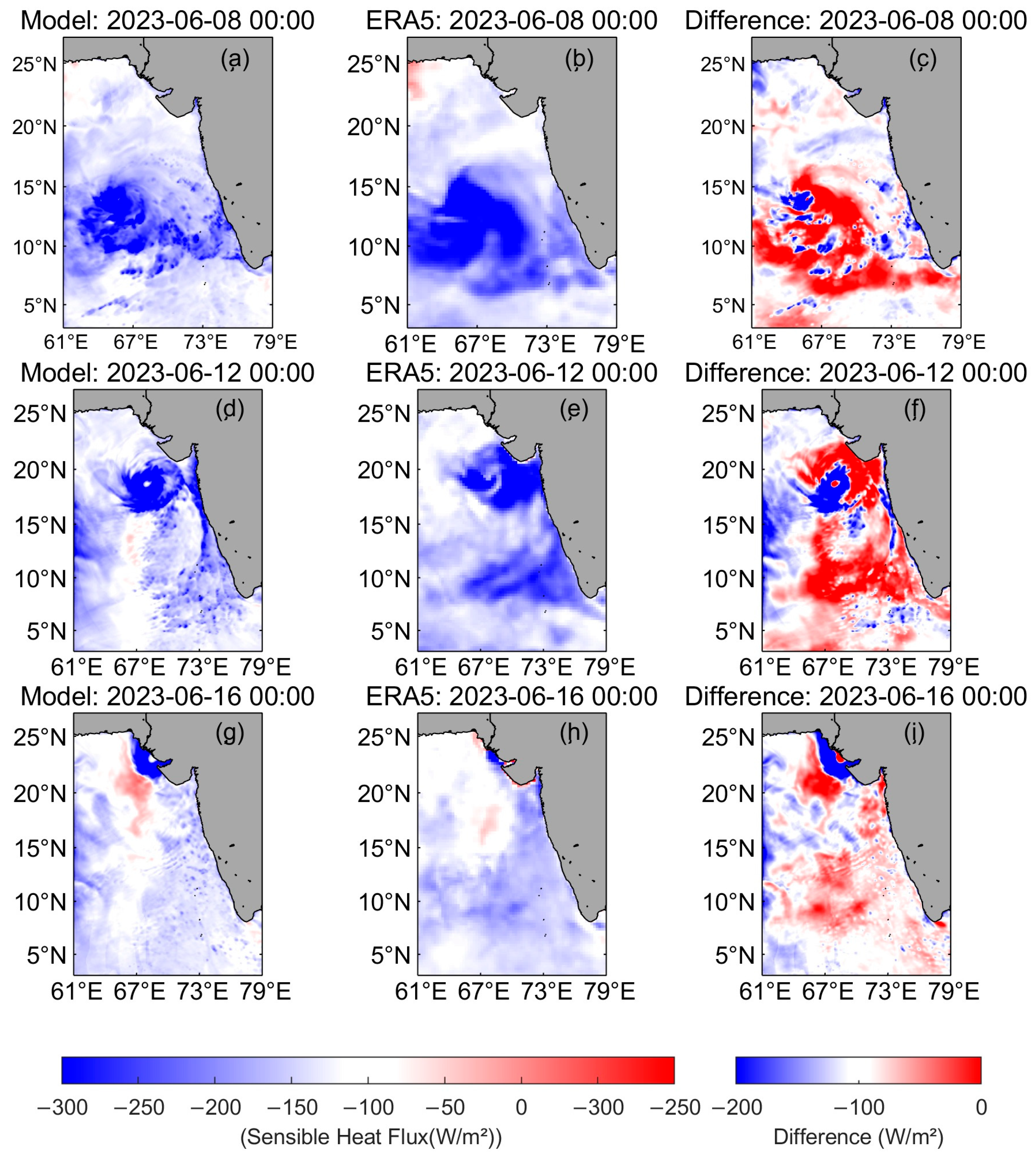
Figure 22 shows the spatial distribution of the surface sensible heat flux obtained by the coupled COAWST model at different times in the Arabian Sea during TC Biparjoy. It can be seen from the figure that the extremum position of the surface sensible heat flux also appears near the center of the TC and is a negative value, which is about −100 W/m2. Away from the center, the surface sensible heat flux can be positive around the value of 25 W/m2.
Table 7 presents the RMSE values of the different experimental surface heat flux results compared to the ERA5 data. The choice of the scalar roughness length scheme exerts a far greater influence on the simulation of surface heat fluxes than the selection of the momentum roughness length scheme. This is evidenced by the significantly larger reduction in the RMSE achieved by switching the thermal and moisture scheme (from Garratt to Fairall) compared to altering the momentum scheme while keeping the thermal and moisture scheme constant. Among the momentum schemes, the Drennan scheme demonstrates stability in terms of sensible heat flux under extreme forcing (June 12), while the Edson scheme performs the best under milder conditions but becomes aggressive during peak intensity. Crucially, within the context of this case study, the relatively lower latent heat flux errors of the Drennan–Fairall2003 combination across all TC stages (Table 7) can be attributed to its consistent and effective parameterization, which performs better than both the Drennan–Garratt and Drennan–Fairall2014 schemes.

4. Discussion

While this study provides insights into the sensitivity of tropical cyclone simulations to surface roughness parameterizations, several limitations should be acknowledged. First, the present work does not account for the effects of sea spray, which can significantly modulate heat and momentum fluxes under high-wind conditions typical of intense tropical cyclones. Second, the parameterization schemes evaluated here, although well-established, may not fully capture the complex, small-scale processes at the air–sea interface during extreme wind events. Third, the model validation relies on satellite and reanalysis data, which themselves contain uncertainties and may have limited spatial and temporal resolution within the highly dynamic core of the cyclone. Furthermore, it should be noted that some of the simulated improvements, while consistent in direction, are of a magnitude comparable to the inherent uncertainties in the observational and reanalysis products used for validation (e.g., best track data, ERA5 fluxes). This underscores the need for caution when interpreting the absolute superiority of one scheme over another, as the differences may, in some metrics, be marginal relative to the error bounds of the reference data. Finally, the coupled model’s performance is influenced by factors such as coupling frequency and spatial resolution, which were not extensively tested in this sensitivity framework.
Addressing these limitations represents an important direction for future research. In particular, incorporating sea spray effects—which mediate heat and momentum exchange across the air–sea interface through wave-breaking processes—could refine the representation of surface fluxes under high-wind conditions. Additionally, exploring higher-resolution wave–atmosphere coupling and testing more advanced parameterizations may further enhance the model’s ability to simulate complex air–sea interactions during tropical cyclones.

5. Conclusions

In this research, the MYNN surface layer scheme of the COAWST model was revised to use simulated wave information regarding the SWAN model to determine the momentum roughness length. The main objectives are to determine the sensitivity of the TC process to different sensitivity experiments and to identify which combinations are closer to the observed data. The main conclusions are as follows:
(1)
Using Copernicus analysis data as the background field and GFS reanalysis wind fields and TPX0 data as driving fields, the simulated TC track, SWH, SST, and other variables from the COAWST atmosphere–ocean–wave coupled model closely match actual measurements. This accuracy suggests that the selection of background fields, initial conditions, and physical parameters is appropriate, indicating that the model performs well in simulating ocean–atmosphere–wave interactions and can serve as a reference for future simulations.
(2)
Based on the comprehensive model simulations and verification against observations, it is concluded that the selection of the momentum roughness length scheme plays a more decisive role in determining the track and intensity forecasts of the typhoon, as well as in the accurate simulation of SWH, compared to the thermal and moisture roughness scheme. Drennan’s parameterization scheme performed comparatively better in these aspects for Cyclone Biparjoy. This is attributed to its more physically realistic representation of the sea surface’s aerodynamic roughness under high-wind conditions, which directly governs the momentum exchange across the air–sea interface. A more accurate drag coefficient leads to an improved simulation of wind stress, which is fundamental for realistically simulating both the atmospheric forcing that steers the typhoon and the energy input for wave growth. Consequently, the relatively good performance in SWH simulation supports the physical credibility of this momentum scheme for this event, confirming its critical role in the coupled atmosphere–ocean–wave model system for tropical cyclone studies.
(3)
The differential performance of the sensitivity experiments across all evaluated aspects can be rationally explained by the corresponding disparities in simulated surface roughness lengths and exchange coefficients. When choosing the physical parameterization scheme, compared with momentum roughness, accurately characterizing thermal and moisture roughness is more crucial for reducing the simulation error of air–sea heat flux under tropical cyclone conditions. Under the condition that the Drennan et al. parameterization scheme provides high accuracy in momentum roughness, sensitivity experiments were conducted for thermal and moisture roughness parameterizations. The results indicate that thermal roughness primarily modulates the efficiency of turbulent heat transfer between the ocean and atmosphere, thereby exerting a limited influence on SST cooling. This effect remains largely confined to the uppermost ocean layer and does not significantly alter the subsurface thermal structure. In the context of a simulated cold SST bias, the Fairall2003 scheme produced more accurate heat flux estimates compared to the Fairall2014 scheme. Comparing this with the ERA5 reanalysis data shows that this scheme increases the RMSE of the flux calculation. These findings underscore that while the thermal and moisture roughness formulation is secondary to momentum roughness in shaping typhoon trajectory and wave simulation, it remains essential for the accurate representation of surface heat fluxes and, consequently, upper ocean thermal responses.
While this study provides insights into the sensitivity of tropical cyclone simulations to surface roughness parameterizations, several limitations should be acknowledged. First, the present work does not account for the effects of sea spray, which can significantly modulate heat and momentum fluxes under high-wind conditions typical of intense tropical cyclones. Second, the parameterization schemes evaluated here, although well-established, may not fully capture the complex, small-scale processes at the air–sea interface during extreme wind events. Third, the model validation relies on satellite and reanalysis data, which themselves contain uncertainties and may have limited spatial and temporal resolution within the highly dynamic core of the cyclone. Finally, the coupled model’s performance is influenced by factors such as coupling frequency and spatial resolution, which were not extensively tested in this sensitivity framework. Addressing these limitations, particularly by incorporating sea spray effects and higher-resolution wave–atmosphere coupling, represents an important direction for future research.
In future research, we will explore the impact of sea spray. Generated by breaking waves under high winds, sea spray mediates the exchange of heat and momentum across the air–sea interface [48]. A modified parameterization scheme will be introduced to better represent the related physical processes under high-wind conditions. This improvement is expected to refine the representation of heat fluxes and consequently enhance the model’s accuracy in simulating complex air–sea interactions.


Author Contributions

Conceptualization, J.C. and J.S.; methodology, X.Y., J.C., and J.S.; formal analysis, X.Y., J.C., and J.S.; writing—original draft preparation, W.Z., Z.W., H.W., and Z.Z.; writing—review and editing, X.Y., J.C., W.Z., and Z.Z.; visualization, X.Y.; supervision, J.C., J.S., and W.Z. All authors have read and agreed to the published version of the manuscript.
Funding

This study was financially supported by the National Natural Science Foundation of China (Grant No. 52271257 and No. 42192552).

Data Availability Statement

The typhoon best track dataset was obtained from the India Meteorological Department (IMD) website (https://rsmcnewdelhi.imd.gov.in, accessed on 7 November 2025). The initial and boundary conditions of the WRF model were derived via the WRF Global Forecast System (GFS) dataset (https://gdex.ucar.edu/datasets/d084001, accessed on 7 November 2025). The heat flux data were obtained from the ERA5 hourly meteorological data (https://cds.climate.copernicus.eu/datasets/reanalysis-era5-single-levels?tab=overview, accessed on 7 November 2025). The topographic data were obtained from the GEBCO bathymetric dataset (https://download.gebco.net/, accessed on 7 November 2025). The initial and boundary conditions required for the ROMS model were obtained from Copernicus Marine Service’s Global Ocean Physics Analysis and Forecast (https://doi.org/10.48670/moi-00016, accessed on 7 November 2025). The Argo float profile data were obtained from the China Argo real-time data center (ftp://ftp.argo.org.cn/pub/ARGO/global/, accessed on 7 November 2025). Satellite fusion OSTIA was used to obtain SST data (https://podaac.jpl.nasa.gov/dataset/OSTIA-UKMO-L4-GLOB-v2.0, accessed on 7 November 2025). Significant wave height data was obtained using the Jason-3 satellite altimeter (https://www.ncei.noaa.gov/data/oceans/jason3/, accessed on 7 November 2025).

Acknowledgments

The authors would like to thank the India Meteorological Department for providing the TC Biparjoy Track dataset, the NCEP for providing the WRF GFS dataset, the CDS for providing the heat flux data, and the China Argo real-time data center for providing the Argo float profile data.

Conflicts of Interest

The authors declare no conflicts of interest.

References

  1. Booij, N.R.R.C.; Ris, R.C.; Holthuijsen, L.H. A third-generation wave model for coastal regions: 1. Model description and validation. J. Geophys. Res. 1999, 104, 7649–7666. [Google Scholar] [CrossRef] [Scilit]
  2. Wu, Z.; Jiang, C.; Deng, B.; Chen, J.; Long, Y.; Qu, K.; Liu, X. Numerical investigation of Typhoon Kai-tak (1213) using a mesoscale coupled WRF-ROMS model. Ocean Eng. 2019, 175, 1–15. [Google Scholar] [CrossRef] [Scilit]
  3. Bauer, P.; Thorpe, A.; Brunet, G. The quiet revolution of numerical weather prediction. Nature 2015, 525, 47–55. [Google Scholar] [CrossRef] [Scilit]
  4. Charnock, H. Wind stress on a water surface. Quart. J. Roy. Meteor. Soc. 1955, 81, 639–640. [Google Scholar] [CrossRef] [Scilit]
  5. Black, P.G.; D’Asaro, E.A.; Drennan, W.M.; French, J.R.; Niiler, P.P.; Sanford, T.B.; Terrill, E.J.; Walsh, E.J.; Zhang, J.A. Air–sea exchange in hurricanes: Synthesis of observations from the coupled boundary layer air–sea transfer experiment. Bull. Am. Meteorol. Soc. 2007, 88, 357–374. [Google Scholar] [CrossRef] [Scilit]
  6. Donelan, M.A.; Haus, B.K.; Reul, N.; Plant, W.J.; Stiassnie, M.; Graber, H.C.; Brown, O.B.; Saltzman, E.S. On the limiting aerodynamic roughness of the ocean in very strong winds. Geophys. Res. Lett. 2004, 31, L18306. [Google Scholar] [CrossRef] [Scilit]
  7. Emanuel, K.A. Sensitivity of tropical cyclones to surface exchange coefficients and a revised steady-state model incorporating eye dynamics. J. Atmos. Sci. 1995, 52, 3969–3976. [Google Scholar] [CrossRef] [Scilit]
  8. Liu, W.T.; Katsaros, K.B.; Businger, J.A. Bulk parameterization of air-sea exchanges of heat and water vapor including the molecular constraints at the interface. J. Atmos. Sci. 1979, 36, 1722–1735. [Google Scholar] [CrossRef] [Scilit]
  9. Montgomery, M.T.; Smith, R.K.; Nguyen, S.V. Sensitivity of tropical cyclone models to the surface drag coefficient. Quart. J. Roy. Meteor. Soc. 2010, 136, 1945–1953. [Google Scholar] [CrossRef] [Scilit]
  10. Bryan, G.H. Effects of surface exchange coefficients and turbulence length scales on the intensity and structure of numerically simulated hurricanes. Mon. Weather Rev. 2012, 140, 1125–1143. [Google Scholar] [CrossRef] [Scilit]
  11. Davis, C.; Wang, W.; Chen, S.S.; Chen, Y.; Corbosiero, K.; DeMaria, M.; Dudhia, J.; Holland, G.; Klemp, J.; Michalakes, J.; et al. Prediction of landfalling hurricanes with the advanced hurricane WRF model. Mon. Weather Rev. 2008, 136, 1990–2005. [Google Scholar] [CrossRef] [Scilit]
  12. Chen, S.S.; Price, J.F.; Zhao, W.; Donelan, M.A.; Walsh, E.J. The CBLAST-Hurricane program and the next-generation fully coupled atmosphere–wave–ocean models for hurricane research and prediction. Bull. Am. Meteorol. Soc. 2007, 88, 311–317. [Google Scholar] [CrossRef] [Scilit]
  13. Alimohammadi, M.; Malakooti, H.; Rahbani, M. Comparison of momentum roughness lengths of the WRF-SWAN online coupling and WRF model in simulation of tropical cyclone Gonu. Ocean. Dyn. 2020, 70, 1531–1545. [Google Scholar] [CrossRef] [Scilit]
  14. Oost, W.A.; Komen, G.J.; Jacobs, C.M.J.; Van Oort, C. New evidence for a relation between wind stress and wave age from measurements during ASGAMAGE. Bound. Layer Meteorol. 2002, 103, 409–438. [Google Scholar] [CrossRef] [Scilit]
  15. Drennan, W.M.; Graber, H.C.; Hauser, D.; Quentin, C. On the wave age dependence of wind stress over pure wind seas. J. Geophys. Res. 2003, 108, 8062. [Google Scholar] [CrossRef] [Scilit]
  16. Taylor, P.K.; Yelland, M.J. The dependence of sea surface roughness on the height and steepness of the waves. J. Phys. Oceanogr. 2001, 31, 572–590. [Google Scholar] [CrossRef] [Scilit]
  17. Bouin, M.N.; Lebeaupin Brossier, C.; Malardel, S.; Voldoire, A.; Sauvage, C. The wave-age-dependent stress parameterisation (WASP) for momentum and heat turbulent fluxes at sea in SURFEX v8. 1. Geosci. Model Dev. 2024, 17, 117–141. [Google Scholar] [CrossRef] [Scilit]
  18. Zhao, Z.; Shi, J.; Wang, H.; Yi, Z.; Zhang, W.; Zhang, X. Parameterization scheme of the sea surface drag coefficient considering the influence of wave states and sea spray stress. Front. Mar. Sci. 2024, 11, 1336709. [Google Scholar] [CrossRef] [Scilit]
  19. Fairall, C.W.; Bradley, E.F.; Hare, J.E.; Grachev, A.A.; Edson, J.B. Bulk parameterization of air–sea fluxes: Updates and verification for the COARE algorithm. J. Clim. 2003, 16, 571–591. [Google Scholar] [CrossRef] [Scilit]
  20. Shi, J.; Zhao, D.; Li, X.; Zhong, Z. New wave-dependent formulae for sea spray flux at air-sea interface. J. Hydrodyn. Ser. B 2009, 21, 573–581. [Google Scholar] [CrossRef] [Scilit]
  21. Shi, J.; Feng, Z.; Sun, Y.; Zhang, X.; Zhang, W.; Yu, Y. Relationship between sea surface drag coefficient and wave state. J. Mar. Sci. Eng. 2021, 9, 1248. [Google Scholar] [CrossRef] [Scilit]
  22. Edson, J.B.; Jampana, V.; Weller, R.A.; Bigorre, S.P.; Plueddemann, A.J.; Fairall, C.W.; Miller, S.D.; Mahrt, L.; Vickers, D.; Hersbach, H. On the exchange of momentum over the open ocean. J. Phys. Oceanogr. 2013, 43, 1589–1610. [Google Scholar] [CrossRef] [Scilit]
  23. Cao, X.; Chen, J.; Shi, J.; Xia, J.; Zhang, W.; Yi, Z.; Wang, H.; Zhang, S.; Lv, J.; Zhao, Z.; et al. Response of Upper Ocean to Parameterized Schemes of Wave Breaking under Typhoon Condition. Remote Sens. 2024, 16, 3524. [Google Scholar] [CrossRef] [Scilit]
  24. Chen, W.; Chen, J.; Shi, J.; Zhang, S.; Zhang, W.; Xia, J.; Wang, H.; Yi, Z.; Wu, Z.; Zhang, Z. Impact of a New Wave Mixing Scheme on Ocean Dynamics in Typhoon Conditions: A Case Study of Typhoon In-Fa (2021). Remote Sens. 2024, 16, 3298. [Google Scholar] [CrossRef] [Scilit]
  25. Wu, Z.; Zou, Z.; Chen, J.; Luo, H.; Deng, B.; Jiang, C.; Lv, Z.; Zhang, H. Dynamic and thermodynamic characteristics of ocean response to super typhoon Mangkhut in the South China Sea. Front. Mar. Sci. 2025, 12, 1586377. [Google Scholar] [CrossRef] [Scilit]
  26. Warner, J.C.; Armstrong, B.; He, R.; Zambon, J.B. Development of a coupled ocean–atmosphere–wave–sediment transport (COAWST) modeling system. Ocean Model. 2010, 35, 230–244. [Google Scholar] [CrossRef] [Scilit]
  27. Hong, S.-Y.; Dudhia, J.; Chen, S.-H. A revised approach to ice microphysical processes for the bulk parameterization of clouds and precipitation. Mon. Wea. Rev. 2004, 132, 103–120. [Google Scholar] [CrossRef] [Scilit]
  28. Iacono, M.J.; Delamere, J.S.; Mlawer, E.J.; Shephard, M.W.; Clough, S.A.; Collins, W.D. Radiative forcing by long-lived greenhouse gases: Calculations with the AER radiative transfer models. J. Geophys. Res. 2008, 113, D13103. [Google Scholar] [CrossRef] [Scilit]
  29. Nakanishi, M.; Niino, H. Development of an improved turbulence closure model for the atmospheric boundary layer. J. Meteorol. Soc. Jpn. Ser. 2009, 87, 895–912. [Google Scholar] [CrossRef] [Scilit]
  30. Tewari, M.; Chen, F.; Wang, W.; Dudhia, J.; LeMone, M.A.; Mitchell, K.; Ek, M.; Gayno, G.; Wegiel, J.; Cuenca, R.H. Implementation and verification of the unified NOAH land surface model in the WRF model. In Proceedings of the 20th Conference on Weather Analysis and Forecasting/16th Conference on Numerical Weather Prediction, Seattle, WA, USA, 12–16 January 2004; Volume 14, pp. 11–15. [Google Scholar]
  31. Grell, G.A. Prognostic evaluation of assumptions used by cumulus parameterizations. Mon. Weather Rev. 1993, 121, 764–787. [Google Scholar] [CrossRef] [Scilit]
  32. Grell, G.A.; Dévényi, D. A generalized approach to parameterizing convection combining ensemble and data assimilation techniques. Geophys. Res. Lett. 2002, 29, 38-1–38-4. [Google Scholar] [CrossRef] [Scilit]
  33. Umlauf, L.; Burchard, H. A generic length-scale equation for geophysical turbulence models. J. Mar. Res. 2003, 61, 235–265. [Google Scholar] [CrossRef] [Scilit]
  34. Warner, J.C.; Sherwood, C.R.; Arango, H.G.; Signell, R.P. Performance of four turbulence closure models implemented using a generic length scale method. Ocean Model. 2005, 8, 81–113. [Google Scholar] [CrossRef] [Scilit]
  35. Weatherall, P.; Ferreras, S.C.; Cardigos, S.D.; Cornish, N.; Davidson, S.R.; Dorschel, B.; Drennon, H.; Ferrini, V.; Harper, H.A.; Isler, T.; et al. The GEBCO_2024 Grid-a Continuous Terrain Model of the Global Oceans and Land; NERC EDS British Oceanographic Data Centre NOC: Liverpool, UK, 2024. [Google Scholar]
  36. Garratt, J.R. The Atmospheric Boundary Layer; Cambridge University Press: Cambridge, UK, 1992; p. 316. [Google Scholar]
  37. Garratt, J.R. The atmospheric boundary layer. Earth Sci. Rev. 1994, 37, 89–134. [Google Scholar] [CrossRef] [Scilit]
  38. Chai, T.; Draxler, R.R. Root mean square error (RMSE) or mean absolute error (MAE)?–Arguments against avoiding RMSE in the literature. Geosci. Model Dev. 2014, 7, 1247–1250. [Google Scholar] [CrossRef] [Scilit]
  39. Hyndman, R.J.; Koehler, A.B. Another look at measures of forecast accuracy. Int. J. Forecast. 2006, 22, 679–688. [Google Scholar] [CrossRef] [Scilit]
  40. Fairall, C.W.; Bradley, E.F.; Rogers, D.P.; Edson, J.B.; Young, G.S. Bulk parameterization of air-sea fluxes for tropical ocean-global atmosphere coupled-ocean atmosphere response experiment. J. Geophys. Res. 1996, 101, 3747–3764. [Google Scholar] [CrossRef] [Scilit]
  41. Edson, J.B.; Zappa, C.J.; Ware, J.A.; McGillis, W.R.; Hare, J.E. Scalar flux profile relationships over the open ocean. J. Geophys. Res. Ocean. 2004, 109, C08S09. [Google Scholar] [CrossRef] [Scilit]
  42. Copernicus Climate Change Service, Climate Data Store. ERA5 Hourly Data on Single Levels from 1940 to Present; Copernicus Climate Change Service (C3S) Climate Data Store (CDS): Bonn, Germany, 2023. [Google Scholar]
  43. Donlon, C.J.; Martin, M.; Stark, J.; Roberts-Jones, J.; Fiedler, E.; Wimmer, W. The operational sea surface temperature and sea ice analysis (OSTIA) system. Remote Sens. 2012, 116, 140–158. [Google Scholar] [CrossRef] [Scilit]
  44. Good, S.; Fiedler, E.; Mao, C.; Martin, M.J.; Maycock, A.; Reid, R.; Roberts-Jones, J.; Searle, T.; Waters, J.; While, J.; et al. The current configuration of the OSTIA system for operational production of foundation sea surface temperature and ice concentration analyses. Remote Sens. 2020, 12, 720. [Google Scholar] [CrossRef] [Scilit]
  45. Desai, S. Jason-3 GPS Based Orbit and SSHA OGDR (PO.DAAC, CA, USA: NASA Physical Oceanography Distributed Active Archive Center). 2016. Available online: https://podaac.jpl.nasa.gov/dataset/JASON_3_L2_OST_OGDR_GPS (accessed on 7 November 2025).
  46. The NCAR Command Language, Version 6.6.2; UCAR/NCAR/CISL/TDD: Boulder, CO, USA, 2019.
  47. Tolman, H.L. Alleviating the garden sprinkler effect in wind wave models. Ocean Model. 2002, 4, 269–289. [Google Scholar] [CrossRef] [Scilit]
  48. Andreas, E.L. Sea spray and the turbulent air-sea heat fluxes. J. Geophys. Res. Oceans. 1992, 97, 11429–11441. [Google Scholar] [CrossRef] [Scilit]
Figure 1. The variables exchanged in the coupled WRF-ROMS-SWAN model.
Jmse 14 00277 g001
Figure 2. Path and intensity of Extremely Severe Cyclonic Storm Biparjoy.
Jmse 14 00277 g002
Figure 3. Map of study area. (a) Location of selected Argo buoys: A1 represents 2902271_151.dat; A2 represents 4903660_006.dat; A3 represents 6903059_364.dat; A4 represents 6990514_006.dat. (b) Jason-3 satellite altimeter track: C1 represents 341_207; C2 represents 342_105; C3 represents 342_168; C4 represents 342_066.
Jmse 14 00277 g003
Figure 4. Comparison of simulated tracks and best track of Extremely Severe Cyclonic Storm Biparjoy.
Jmse 14 00277 g004
Figure 5. Comparison of TC central pressure from models and IMD best track dataset.
Jmse 14 00277 g005
Figure 6. Comparison of maximum sustained wind velocity from models and IMD best track dataset.
Jmse 14 00277 g006
Figure 7. An SST comparison between the Drennan−Garratt experiment and OSTIA data. The left column (a,d,g) represents the results of the Drennan–Garratt scheme, the middle column (b,e,h) represents the results of the OSTIA data, and the right column (c,f,i) represents the difference between the model and OSTIA data.
Jmse 14 00277 g007
Figure 8. Comparison of temperature profiles between four momentum roughness length scheme experiments and buoy measurements for (a) Buoy 2902271; (b) Buoy 4903660; (c) Buoy 6903059; (d) Buoy 6990514.
Jmse 14 00277 g008
Figure 9. Comparison of temperature profiles between three thermal and moisture roughness length scheme experiments and buoy measurements for (a) Buoy 2902271; (b) Buoy 4903660; (c) Buoy 6903059; (d) Buoy 6990514.
Jmse 14 00277 g009
Figure 10. Simulated significant wave height (m) for the Drennan–Garratt scheme on (a) 11 June 2023; (b) 12 June 2023; (c) 13 June 2023; (d) 14 June 2023; (e) 15 June 2023; (f) 16 June 2023.
Jmse 14 00277 g010
Figure 11. Simulated swell wave height (m) for Drennan–Garratt scheme on (a) 11 June 2023; (b) 12 June 2023; (c) 13 June 2023; (d) 14 June 2023; (e) 15 June 2023; (f) 16 June 2023.
Jmse 14 00277 g011
Figure 12. Evaluation of Drennan–Garratt-simulated SWH data against observations from Jason3 satellite (ad).
Jmse 14 00277 g012
Figure 13. Simulated momentum roughness lengths (m): (ac) Taylor–Garratt; (df) Drennan–Garratt; (gi) OOST–Garratt; (jl) Edson–Garratt.
Jmse 14 00277 g013
Figure 14. The same as Figure 13 but for the simulated drag coefficients (Cd): (ac) Taylor–Garratt; (df) Drennan–Garratt; (gi) OOST–Garratt; (jl) Edson–Garratt.
Jmse 14 00277 g014
Figure 15. The same as Figure 13 but for the simulated thermal roughness lengths (m): (ac) Taylor–Garratt; (df) Drennan–Garratt; (gi) OOST–Garratt; (jl) Edson–Garratt.
Jmse 14 00277 g015
Figure 16. The same as Figure 13 but for the simulated moisture roughness lengths (m): (ac) Taylor–Garratt; (df) Drennan–Garratt; (gi) OOST–Garratt; (jl) Edson–Garratt.
Jmse 14 00277 g016
Figure 17. The same as Figure 13 but for the simulated enthalpy exchange coefficient (Ck): (ac) Taylor–Garratt; (df) Drennan–Garratt; (gi) OOST–Garratt; (jl) Edson–Garratt.
Jmse 14 00277 g017
Figure 18. The same as Figure 13 but for the ratio of enthalpy to momentum exchange coefficients (Ck/Cd): (ac) Taylor–Garratt; (df) Drennan–Garratt; (gi) OOST–Garratt; (jl) Edson–Garratt.
Jmse 14 00277 g018
Figure 19. The same as Figure 13 but for the simulated 10 m wind speed: (ac) Taylor–Garratt; (df) Drennan–Garratt; (gi) OOST–Garratt; (jl) Edson–Garratt.
Jmse 14 00277 g019
Figure 20. The same as Figure 13 but for simulated momentum flux (kg/(m·s2)): (ac) Taylor–Garratt; (df) Drennan–Garratt; (gi) OOST–Garratt; (jl) Edson–Garratt.
Jmse 14 00277 g020
Figure 21. The spatial distribution of the surface latent heat flux influenced by TC Biparjoy based on the Drennan–Garratt scheme. The left column (a,d,g) represents the results of the Drennan–Garratt scheme, the middle column (b,e,h) represents the results of the ERA5 data, and the right column (c,f,i) represents the difference between the model and ERA5 data.
Jmse 14 00277 g021
Figure 22. The spatial distribution of the surface sensible heat flux influenced by TC Biparjoy based on the Drennan–Garratt scheme. The left column (a,d,g) represents the results of the Drennan–Garratt scheme, the middle column (b,e,h) represents the results of the ERA5 data, and the right column (c,f,i) represents the difference between the model and ERA5 data.
Jmse 14 00277 g022
Table 1. Parameterization scheme in WRF model.
Physics OptionsParameterization Scheme
mp_physicsWSM 5-class graupel scheme [27]
ra_lw_physicsRRTMG scheme [28]
ra_sw_physicsRRTMG scheme [28]
sf_sfclay_physicsMYNN surface layer scheme [29]
sf_surface_physicsNoah Land Surface Model [30]
bl_pbl_physicsMYNN2.5 scheme [29]
cu_physicsGrell 3D scheme [31,32]
Table 2. Parameterization scheme of different experiments.
Name for ExperimentsMomentum Roughness Length Scheme (z0)Thermal and Moisture Roughness Length Scheme (zt, zq)
Taylor–GarrattTaylor and Yelland [16]Garratt [36,37]
Drennan–GarrattDrennan [15]Garratt
OOST–GarrattOost [14]Garratt
Edson–GarrattEdson [22]Garratt
Drennan–Fairall2003DrennanFairall et al. 2003 [19]
Drennan–Fairall2014DrennanFairall et al. formulation (via COARE3.5 in COAWST) [26]
Table 3. Error analysis for TC track, central pressure, and maximum sustained wind velocity.
Name for ExperimentsMAE of TC Track (km)RMSE of TC Central Pressure (hpa)RMSE of Maximum Sustained Wind Velocity (m/s)
Taylor–Garratt91.11785.10905.9934
Drennan–Garratt72.03335.44796.1813
OOST–Garratt88.22044.97676.0951
Edson–Garratt83.40005.95056.4775
Drennan–Fairall200383.97635.14415.6643
Drennan–Fairall201481.52424.24775.3055
Table 4. Difference between simulated SST values and OSTIA values during TC development process.
Name for ExperimentsSST RMSE on 8 JuneSST RMSE on 12 JuneSST RMSE on 16 June
Taylor–Garratt0.57200.69220.6318
Drennan–Garratt0.56590.68580.6180
OOST–Garratt0.57380.69260.6331
Edson–Garratt0.58020.70020.6354
Drennan–Fairall20030.57480.67830.6268
Drennan–Fairall20140.58030.68300.6353
Table 5. Comparison of model temperature simulations with Argo float: MAE and SLTE.
Main Statistical ParametersBuoy IDTaylor–GarrattTaylor–GarrattDrennan–GarrattOOST–GarrattEdson–GarrattDrennan–Fairall2003Drennan–Fairall2014
MAE29022710.4560.4560.45020.45430.45310.44910.4508
49036600.34380.34380.34120.330.33830.33750.3386
69030590.28360.28360.28720.28320.28460.2870.2869
69905140.39920.39920.39650.38450.39320.39260.3938
SLTE2902271−0.3777−0.3777−0.4214−0.41−0.3806−0.3791−0.3878
4903660−0.1244−0.1244−0.12−0.1059−0.168−0.0953−0.1342
6903059−0.3426−0.3426−0.1545−0.2863−0.336−0.121−0.1546
Table 6. Comparison of model SWH simulations with Jason3 data: MAE and MAPE.
Name for ExperimentsMAEMAPE
341_207342_105342_168342_066341_207342_105342_168342_066
Taylor–Garratt0.67250.58250.80320.810926.194123.080018.864418.9144
Drennan–Garratt0.57160.44300.62721.181622.562217.675415.582327.4078
OOST–Garratt0.60020.51930.72790.865323.398721.510816.748919.8586
Edson–Garratt0.62800.45590.67240.710124.612719.762014.482916.1913
Drennan–Fairall20030.59970.42160.74380.997523.894521.146414.463023.6012
Drennan–Fairall20140.63110.38990.76211.184024.788121.251112.962327.4704
Table 7. Comparison of model surface heat flux simulations with ERA5.
Name for ExperimentsRMSE of Latent Heat FluxRMSE of Sensible Heat Flux
8 June12 June16 June8 June12 June16 June
Taylor–Garratt60.3574.8465.4111.3719.5212.48
Drennan–Garratt61.9672.1164.5612.3217.9312.85
OOST–Garratt63.9476.0268.3512.1619.0512.62
Edson–Garratt59.4977.3265.2111.0419.1313.07
Drennan–Fairall200356.7465.2662.0612.7316.2212.14
Drennan–Fairall201454.7667.5763.5612.9818.1713.22
Disclaimer/Publisher’s Note: The statements, opinions and data contained in all publications are solely those of the individual author(s) and contributor(s) and not of MDPI and/or the editor(s). MDPI and/or the editor(s) disclaim responsibility for any injury to people or property resulting from any ideas, methods, instructions or products referred to in the content.