The Neural Network Fitting Method for Green’s Function of Finite Water Depth

Abstract

In marine hydrodynamics, the core of the boundary element method (BEM) lies in the numerical calculation of the free-surface Green’s function. With the rise of artificial intelligence, using neural networks to fit Green’s function has become a new trend, yet most existing studies are confined to fitting Green’s function in infinite water depth. In this paper, a neural network fitting method for a finite-depth Green’s function is proposed. The classical Multilayer Perceptron (MLP) network and the emerging Kolmogorov–Arnold Network (KAN) are employed to conduct global and partition-based fitting experiments. Experiments indicate that the partition-based KAN fitting model achieves higher fitting accuracy, with most regions reaching 4D fitting precision. For large-scale data input, the average time for the model to calculate a single Green’s function value is 0.0868 microseconds, which is significantly faster than the 0.1120 s required by the traditional numerical integration method. These results demonstrate that the KAN can serve as an accurate and efficient model for finite-depth Green’s functions. The proposed KAN-based fitting method not only reduces the computational cost of numerical evaluation of Green’s functions but also maintains high prediction precision, providing an alternative approach to accelerate BEM calculations for floating body hydrodynamic analysis.

1. Introduction

In the field of ocean engineering, wave–body interaction is an important research topic, and the hydrodynamic performance of floating bodies is of great significance to their operational stability and reliability. Potential flow theory serves as the basic theory for analyzing the interaction between floating bodies and waves, with the Boundary Element Method (BEM) being the primary solution algorithm. Based on different calculation models, it can be divided into the distributed source method [1] and the source couple mixed distribution method [2]. Regardless of the adopted calculation method, the numerical computation of Green’s function is the most crucial step, which directly affects the accuracy and efficiency of BEM in solving hydrodynamic performance problems. According to the different panel discretization approaches for flow fields, the Green’s function can be divided into the simple Green’s function and the free-surface Green’s function. The free-surface Green’s function is one of the key terms in hydrodynamic research [3]. When using BEM to solve the hydrodynamic performance of large offshore engineering structures, the computational scale of the free-surface Green’s function reaches approximately $5\times {10}^7$ evaluations. Therefore, the computational accuracy and efficiency of the free-surface Green’s function directly determine the accuracy and efficiency of the BEM program. An excellent BEM program should strike a balance between appropriate accuracy and high computational efficiency.

Based on the water depth conditions of floating bodies, the free-surface Green’s function can be classified into the infinite-water-depth free-surface Green’s function and the finite-water-depth free-surface Green’s function. Since the infinite-water-depth free-surface Green’s function is not restricted by bottom boundary conditions, its calculation is relatively straightforward, and the corresponding calculation methods have been well-established. Common methods for calculating the infinite-water-depth Green’s function include the Romberg integration method [4], the Chebyshev polynomial approximation method [5,6,7,8], the series expansion method [9], the global approximation method [10], etc. In recent years, with the rapid development of artificial intelligence, the application of neural networks in the fitting of the infinite-water-depth Green’s function has been gradually increasing. For instance, studies have employed a Multilayer Perceptron (MLP) network trained with 16D precision data [11] and other machine learning-based approaches [12,13].

Due to the influence of bottom boundary conditions, the finite-water-depth Green’s function will be more complex to solve, with two primary approaches: series solution and numerical integration solution. John [14] proposed a series expression for the finite-water-depth Green’s function. The series expression offers high computational efficiency but exhibits singularities in the near-field region; thus, it is typically applied to the far field, while the near field can only be solved via numerical integration with low computational efficiency. Newman [5] investigated the demarcation criterion between the near field and far field, determining the boundary as R/h = 1/2 (where R denotes the horizontal distance, and h represents the water depth). Similarly to the infinite-water-depth scenario, the integral solution of the finite-water-depth Green’s function also comprises three components, namely the fundamental solution term, the analytical imaginary part, and a semi-infinite Cauchy principal value integral term containing singular points. However, the principal value integral expression in the case of finite water depth is more intricate and challenging to solve. The main methods to solve the principal value integral of the finite-water-depth Green’s function include the Gauss–Laguerre integration method and the Chebyshev polynomial fitting method. Endo [15] proposed the Gauss–Laguerre integration method, which decomposes the principal value integral into a Gauss–Laguerre integral without singularity and an exponential integral, which is equivalent to transferring the singularity in the original expression to the exponential integral function. However, this method needs at least 64 Gaussian nodes to meet the accuracy requirements and suffers from a high-frequency distortion problem. In response to these problems, Liu [16] improved the traditional Gauss–Laguerre integration method by splitting the integrand into a Gauss–Laguerre integral and a principal integral of the infinite-water-depth Green’s function, which is equivalent to transferring the singular point to the principal integral of the infinite-water-depth Green’s function. The latter calculation has been well-established. Using this improved method, only 15 Gaussian nodes are needed to achieve satisfactory accuracy, and the problem of high-frequency distortion is alleviated to a certain extent. Yang [17] further improved the Gauss–Laguerre integration method on the basis of Liu’s research and treated all exponential function terms that would cause high-frequency distortion in the same way as Liu, further reducing the numerical error. Shan [18] systematically summarized the Gauss–Laguerre integration method, including the solution algorithm for the principal value integral component of the finite-water-depth Green’s function, and adopted OpenMP parallelization technology to enhance the computational efficiency. Liu [19] analyzed the strange frequency problem of the Gauss–Laguerre integration method and proposed an enhancement method to mitigate this issue, providing a foundation for subsequent research. Although the numerical integration method is simple and intuitive, its solution efficiency is not high. Hydrodynamic software tends to adopt the Chebyshev polynomial fitting method to ensure high accuracy and satisfactory computational speed. Newman [5] reduced the solution of the principal value integral part of the finite-water-depth Green’s function to the calculation of a dimensionless auxiliary function $L\left(X,V,H\right)$, and used Chebyshev polynomials to fit the smooth variation in the function’s residual component, developing a package called FINGREEN, but he did not describe the implementation details of the algorithm in detail. Chen [20] implemented a method similar to Newman’s framework, using Chebyshev polynomials to fit the finite-water-depth Green’s function and providing specific implementation details. This algorithm serves as the computational core of Hydrostar. Mackay [21] found that the numerical value of Newman and Chen’s method fluctuates significantly at low Kh (dimensionless wave number), and the integral limits when K tends to 0 and infinity are inconsistent with those of the Green’s function expression. Therefore, he proposed a consistency expression that varies more slowly with Kh, making it easier to fit using triple Chebyshev polynomials. Although the Chebyshev polynomial fitting method offers high computational efficiency, its implementation is much more complex than that of direct but slow numerical integration algorithms, requiring profound knowledge of computational mathematics and a lot of debugging work. A critical limitation in current marine hydrodynamic analysis lies in the lack of accurate and efficient AI-based representations for the finite-water-depth Green’s functions, which restricts the further improvement of computational efficiency and precision in relevant engineering applications. This research direction aligns with the prediction that AI algorithms would be gradually introduced to marine hydrodynamic and marine structure analysis, with new hybrid models emerging as a key research frontier [22]. This is precisely the objective of the present study.

Machine learning, as the core of artificial intelligence, encompasses a variety of computer algorithms that can be automatically optimized through experience and data, such as support vector machines (SVMs) and neural networks. Due to the benefits of their powerful nonlinear modeling capability, neural networks have been widely favored by researchers in various fields. Hornik [23] proposed the Universal Approximation Theorem, which states that a feedforward neural network with a single hidden layer—provided the hidden layer has a sufficient number of neurons and uses appropriate nonlinear activation functions (such as Sigmoid, ReLU, etc.)—can approximate any continuous function defined on a compact set with arbitrary accuracy. This theorem provides a mathematical basis for the classical MLP network. In order to solve the “curse of dimensionality” problem of MLP networks, Liu [24] et al., inspired by the Kolmogorov–Arnold Representation Theorem, proposed Kolmogorov–Arnold Networks (KAN), which can better fit high-dimensional data. Deep learning is the second wave of machine learning. Hinton [25] pointed out that the multi-hidden-layer neural network has excellent feature learning ability. Its essence is that the deep neural network can automatically learn a multi-level abstract representation from data through hierarchical feature extraction and nonlinear transformation, and ultimately improve the accuracy of the results.

Previous machine learning studies on the pulsating source Green’s function have been confined to the infinite water depth scenario. For finite water depth conditions, calculations mainly rely on numerical integration methods or polynomial approximation methods based on analytical functions. The former has high accuracy but requires time-consuming calculation, while the latter is efficient but complex to implement. Drawing on Mackay’s consistent expression for the finite-water-depth Green’s function [21], this paper employs the numerical integration method to construct high-precision databases for auxiliary functions $L$, $\partial L/\partial A$, $\partial L/\partial B_1$, and $\partial L/\partial B_2$, all of which are associated with the finite-water-depth Green’s function. These datasets are then used to train both the MLP network and the KAN. Model parameters are updated iteratively via the backpropagation algorithm, with hyperparameters (e.g., network depth and width) adjusted to optimize performance. The neural network prediction models for fitting the auxiliary functions $L$, $\partial L/\partial A$, $\partial L/\partial B_1$, and $\partial L/\partial B_2$ are thus established. The value of the finite-water-depth Green’s function can be derived from the predicted values of these auxiliary functions. Research findings demonstrate that the partition-based prediction model for the Green’s function based on the KAN can simultaneously ensure high accuracy and computational efficiency, providing a novel approach for the numerical evaluation of the finite-water-depth Green’s function.

2. Methodology

The core work of this paper is to employ neural networks to fit the auxiliary function associated with the finite-water-depth Green’s function, thereby avoiding the inefficiency of traditional numerical integration methods and the complexity of polynomial approximation approaches. The research involves three key theoretical frameworks: potential flow theory, Green’s function method, and neural network theory.

2.1. Potential Flow Theory

In the analysis of wave–body interaction, the viscosity of the fluid can be neglected under certain conditions, and the flow can be approximately regarded as incompressible and irrotational; thus, potential flow theory is applicable to solve such problems. The potential flow method employed in this study is applicable to linear frequency-domain analysis, reduced-order time-domain analysis (via frequency-domain to time-domain conversion, such as inverse Fourier transform), and can be extended to weakly nonlinear cases with appropriate modifications (e.g., incorporating weakly nonlinear free-surface boundary conditions). For full-order time-domain analysis involving strong nonlinearities, the potential flow method is subject to limitations due to the neglect of viscosity and the simplification of boundary conditions. The wave–body interaction system can be modeled as a 6-DOF oscillatory system, which satisfies the equation expressed in Equation (1):

$${\sum }_{j=1}^6\left(M_{kj}+A_{kj}\right)\ddot{x_j}+B_{kj}\dot{x_j}+C_{kj}{x}_j=F_k, k=\mathrm{1,2},\dots ,6$$

(1)

where $M$ denotes the inertia matrix; $A$ and $B$ represent the added mass matrix and damping coefficient matrix, respectively (collectively referred to as the hydrodynamic coefficient matrix); $\mathrm{C}$ is the coefficient matrix of the hydrostatic restoring force; $F_k$ stands for the wave-induced force vector; and $x_j$ is the motion response vector of the floating body. It is easy to obtain the mass of a floating body and the coefficient of a hydrostatic restoring force. In contrast, the hydrodynamic coefficients and wave-induced force—parameters closely related to the hydrodynamic performance of the floating body—are the core and difficult-to-solve components in the wave–body interaction analysis.

In potential flow theory, the flow velocity of the fluid can be described by the velocity potential, and the continuity equation of the flow can be converted into the Laplace equation. By solving the Laplace equation with corresponding boundary conditions, the velocity potential of the fluid can be obtained. On this basis, other key hydrodynamic parameters—including the hydrodynamic coefficients and wave-induced forces mentioned earlier—can be derived through further calculations. Therefore, the problem of potential flow theory is essentially a boundary value problem of the Laplace equation. According to the radiation-diffraction theory, the unsteady spatial velocity complex potential $\varphi$ for the interaction between a floating body and waves is the superposition of incident potential, radiation potential, and diffraction potential, as expressed in Equation (2):

$$\varphi ={\varphi }_0+\sum _{i=1}^6{\varphi }_i+{\varphi }_7$$

(2)

where ${\varphi }_0$ denotes the incident potential, which is usually a known quantity derived from the given wave conditions; ${\varphi }_i$ (i = 1, 2, …, 6) represent the radiation potentials corresponding to the six 6-DOF oscillation modes of the floating body, respectively; and ${\varphi }_7$ is the diffraction potential induced by the wave scattering around the floating body. Among these, the radiation potential and diffraction potential are the difficult-to-solve components in the velocity potential decomposition. For a floating body with zero forward speed, the diffraction potential can be derived indirectly through radiation potential by applying the Haskind relation—a key theoretical relation in marine hydrodynamics. Therefore, solving the radiation potential becomes the core to addressing the wave–body interaction problem under zero-speed conditions. The radiation potential under finite water depth conditions satisfies the Laplace equations expressed in Equation (3):

$$\begin{array}{c}\left\{\begin{array}{ll}\mathrm{\Delta }{\varphi }_i=0,& \mathrm{in} \mathrm{z} < 0\\ {\displaystyle \frac{\partial {\varphi }_i}{\partial z}}-K{\varphi }_i=0,& \mathrm{on} \mathrm{z} = 0\\ {\left.{\displaystyle \frac{\partial {\varphi }_i}{\partial n}}\right|}_S=n_i,& \mathrm{on} \mathrm{S}\\ {\left.{\displaystyle \frac{\partial {\varphi }_i}{\partial z}}\right|}_{z=-h}=0,& \mathrm{on} \mathrm{z} = -\mathrm{h}\\ \underset{R\to \mathrm{\infty }}{\mathrm{l}\mathrm{i}\mathrm{m}}\sqrt{R}\left({\displaystyle \frac{\partial {\varphi }_i}{\partial R}}-i{k}_0{\varphi }_i\right)=0,& \mathrm{radiation} \mathrm{conditions}\end{array}\right.\end{array}$$

(3)

where $n_i$ is the ith unit normal vector directed into the fluid on the wetted surface S of the body. $K={\omega }^2/g$ and $k_0$ denote wave numbers under infinite and finite water depth conditions, respectively. When the water depth is h, both satisfy the dispersion equation expressed in Equation (4):

$$k_0\mathrm{t}\mathrm{a}\mathrm{n}\mathrm{h}{k}_{0}h=K$$

(4)

From the system of Equation (3), it is difficult to obtain the analytical solution. It can be transformed into the boundary integral equation as expressed in Equation (5) by employing the Green’s function method, and then the numerical solution can be obtained by applying the boundary element method.

$${\mathrm{\varphi }}_i\left(P\right)={\displaystyle \frac{1}{4\mathrm{\pi }}}{\iint }_S\left[G\left(P,Q\right)\widetilde{n_i}-{\mathrm{\varphi }}_i\left(Q\right){\displaystyle \frac{\partial \mathrm{G}\left(P,Q\right)}{\partial \mathrm{n}}}\right]dS$$

(5)

Under the condition of finite water depth, the solution of the free-surface Green’s function $G\left(P,Q\right)$ and its directional derivative $\partial G\left(P,Q\right)/\partial n$ poses a key challenge in the practical application of the boundary element method.

2.2. Green’s Function in Finite Water Depth

The finite depth Green’s function physically represents the velocity potential at a field point induced by a unit source in an ideal fluid domain with a finite water depth, which serves as the fundamental kernel for solving boundary integral equations in marine hydrodynamic problems. Its numerical evaluation is computationally expensive, mainly due to the need to handle the oscillatory and singular integral terms arising from the free surface boundary condition and seabed constraint, as well as the iterative summation of infinite series for satisfying the far-field radiation condition. Tavakoli [26] pointed out that transient and non-transient Green’s functions can be used for modeling floating bodies. The non-transient Green’s function is adopted in this study primarily because our research focuses on the steady-state hydrodynamic response of floating structures under regular wave excitation. This formulation avoids the additional computational burden of time-domain integration required for transient Green’s functions, while ensuring sufficient accuracy for the steady-state analysis objectives of the present work.

Under the condition of water depth h, the finite-water-depth Green’s function $G\left(P,Q\right)=G\left(x,y,z;\xi ,\eta ,\zeta \right)$ satisfies Equation (6):

$$\left\{\begin{array}{l}\mathrm{\Delta }G=\delta \left(P,Q\right)\\ {\displaystyle \frac{\partial G}{\partial z}}-KG=0\\ {\displaystyle \frac{\partial G}{\partial z}}{|}_{z=-h}=0\\ \underset{R\to \mathrm{\infty }}{\mathrm{l}\mathrm{i}\mathrm{m}}\sqrt{R}\left({\displaystyle \frac{\partial G}{\partial R}}-i{k}_{0}G\right)=0\end{array}\right.$$

(6)

The coordinates of the field point $P$ and the source point $Q$ are $\left(x,y,z\right)$ and $\left(\xi ,\eta ,\zeta \right)$, respectively. Wehausen and Laitone [27] gave the integral expression for the finite-water-depth Green’s function

$$G={\displaystyle \frac{1}{r}}+{\displaystyle \frac{1}{r_2}}+{\int }_0^{\mathrm{\infty }}{\displaystyle \frac{2\left(k+K\right)\mathrm{c}\mathrm{o}\mathrm{s}\mathrm{h}\left(k\left(z+h\right)\right)\mathrm{c}\mathrm{o}\mathrm{s}\mathrm{h}\left(k\left(\zeta +h\right)\right)}{k\mathrm{s}\mathrm{i}\mathrm{n}\mathrm{h}\left(kh\right)-K\mathrm{c}\mathrm{o}\mathrm{s}\mathrm{h}\left(kh\right)}}{e}^{-kh}{J}_0\left(kR\right)\mathrm{d}k$$

(7)

where $r=\sqrt{R^2+(z-\zeta {)}^2}$, $r_2=\sqrt{R^2+(z+\zeta +2h{)}^2}$, $R=\sqrt{(x-\xi {)}^2+(y-\eta {)}^2}$, and $J_0$ is the Bessel function of order 0 of the first kind. Notably, the integral term is a complex contour integral that bypasses the poles from below.

The third term of the integral expression (7) is a semi-infinite integral characterized by both singularity and high-frequency oscillations. The actual treatment should be interpreted as a contour integral bypassing the singularity. Bypassing the singular points generates an imaginary part due to the half-residue contribution. This imaginary part is analytical and does not pose a challenge in the solution process, while the real part contains a Cauchy Principal Value Integral, as expressed in Equation (8), which is the core bottleneck in solving the finite-water-depth Green’s function

$$\mathrm{R}\mathrm{e}\left(G\right)={\displaystyle \frac{1}{r}}+{\displaystyle \frac{1}{r_2}}+\mathrm{P}\mathrm{V}{\int }_0^{\mathrm{\infty }}{\displaystyle \frac{2\left(k+K\right)\mathrm{c}\mathrm{o}\mathrm{s}\mathrm{h}\left(k\left(z+h\right)\right)\mathrm{c}\mathrm{o}\mathrm{s}\mathrm{h}\left(k\left(\zeta +h\right)\right)}{k\mathrm{s}\mathrm{i}\mathrm{n}\mathrm{h}\left(kh\right)-K\mathrm{c}\mathrm{o}\mathrm{s}\mathrm{h}\left(kh\right)}}{e}^{-kh}{J}_0\left(kR\right)\mathrm{d}k$$

(8)

Mackay [21] non-dimensionalized Equation (8) and derived a consistent expression. Equations (9)–(16) present the associated derivation steps. For detailed derivations, refer to the original paper. A dimensionless parameter is

$$\mathrm{A}={\displaystyle \frac{\mathrm{R}}{\mathrm{h}}},{\mathrm{B}}_{\mathrm{j}}={\displaystyle \frac{{\mathrm{v}}_{\mathrm{j}}}{\mathrm{h}}},\mathrm{X}=\mathrm{K}\mathrm{R},{\mathrm{V}}_{\mathrm{j}}=\mathrm{K}{\mathrm{v}}_{\mathrm{j}},\mathrm{H}=\mathrm{K}\mathrm{h}$$

(9)

where $v_1=\left|z-\zeta \right|$, $v_2=z+\zeta +2h$, $v_3=\left|z+\zeta \right|$, $v_4=z-\zeta +2h$, $v_5=\zeta -z+2h$, and $v_6=z+\zeta +4h$.

$$\left\{\begin{array}{l}f\left(u,H\right)={\displaystyle \frac{u+H}{\left(u-H\right)-\left(u+H\right)e^{-2u}}}\\ g\left(u,H\right)={\displaystyle \frac{(u+H{)}^2}{(u-H{)}^2-(u^2-H^2)e^{-2u}}}\end{array}\right.$$

(10)

$$\left\{\begin{array}{l}{G}_1\left(A,B,H\right)=\mathrm{P}\mathrm{V}{\int }_0^{\mathrm{\infty }}\left[f\left(u,H\right)-1\right]\left[e^{-u\left(2+B\right)}+e^{-u\left(2-B\right)}\right]J_0\left(uA\right)\mathrm{d}u\\ G_2\left(A,B,H\right)=\mathrm{P}\mathrm{V}{\int }_0^{\mathrm{\infty }}\left\{\left[f\left(u,H\right)-1\right]e^{-u\left(2+B\right)}+g\left(u,H\right)e^{-u\left(4-B\right)}\right\}{J}_0\left(uA\right)\mathrm{d}u\end{array}\right.$$

(11)

$$G_1\left(A,B,H\right)=\left\{\begin{array}{ll}{L}_1\left(A,B,H\right)+L_2\left(H\right)& ,H\le 1\\ L_3\left(A,B,H\right)-{\displaystyle \frac{2}{\sqrt{A^2+(2+B{)}^2}}}-{\displaystyle \frac{2}{\sqrt{A^2+(2-B{)}^2}}}& ,H>1\end{array}\right.$$

(12)

$$G_2\left(A,B,H\right)=\left\{\begin{array}{ll}{M}_1\left(A,B,H\right)+M_2\left(H\right)& ,H\le 1\\ M_3\left(A,B,H\right)-{\displaystyle \frac{2}{\sqrt{A^2+(2+B{)}^2}}}& ,H>1\end{array}\right.$$

(13)

$$\left\{\begin{array}{l}{L}_1\left(A,B,H\right)=\mathrm{P}\mathrm{V}{\int }_0^{\mathrm{\infty }}\left[f\left(u,H\right)-1\right]\left\{\left[e^{-u\left(2+B\right)}+e^{-u\left(2-B\right)}\right]J_0\left(uA\right)-2e^{-2u}\right\}\mathrm{d}u\\ L_2\left(H\right)=\mathrm{P}\mathrm{V}{\int }_0^{\mathrm{\infty }}\left[f\left(u,H\right)-1\right]2e^{-2u}\mathrm{d}u\\ L_3\left(A,B,H\right)=\mathrm{P}\mathrm{V}{\int }_0^{\mathrm{\infty }}\left[f\left(u,H\right)+1\right]\left[e^{-u\left(2+B\right)}+e^{-u\left(2-B\right)}\right]J_0\left(uA\right)\mathrm{d}u\\ M_1\left(A,B,H\right)=\mathrm{P}\mathrm{V}{\int }_0^{\mathrm{\infty }}\left\{\left[f\left(u,H\right)-1\right]\left[e^{-u\left(2+B\right)}{J}_0\left(uA\right)-e^{-3u}\right]+g\left(u,H\right)\left[e^{-u\left(4-B\right)}{J}_0\left(uA\right)-e^{-3u}\right]\right\}\mathrm{d}u\\ M_2\left(H\right)=\mathrm{P}\mathrm{V}{\int }_0^{\mathrm{\infty }}\left[f\left(u,H\right)-1+g\left(u,H\right)\right]e^{-3u}\mathrm{d}u\\ M_3\left(A,B,H\right)=\mathrm{P}\mathrm{V}{\int }_0^{\mathrm{\infty }}\left\{\left[f\left(u,H\right)+1\right]e^{-u\left(2+B\right)}+g\left(u,H\right)e^{-u\left(4-B\right)}\right\}{J}_0\left(uA\right)\mathrm{d}u\end{array}\right.$$

(14)

The $f\left(u,H\right)$ and $g\left(u,H\right)$ functions presented in Equation (10) exhibit a singular point near $u=H$, so the six functions $L_i\left(i=1,2,3\right)$ and $M_i\left(i=1,2,3\right)$ in Equation (14) are the principal value integral functions, whose numerical values can be solved by employing the vectorized adaptive integration method [28] along the complex path $\left[0,H+i,H+1,\mathrm{\infty }\right]$. Then, $G_1\left(A,B,H\right)$ and $G_2\left(A,B,H\right)$ in Equations (12) and (13) can be further derived. On this basis, the auxiliary function $L\left(A,B_1,B_2,H\right)$ associated with the real part of the Green’s function can be finally obtained

$$L\left(A,B_1,B_2,H\right)=\left\{\begin{array}{ll}{G}_1\left(A,B_1,H\right)+G_1\left(A,B_2,H\right)& 0\le B_2\le 1\\ G_1\left(A,B_1,H\right)+G_2\left(A,B_2,H\right)+H\cdot F\left(H\cdot A,H\cdot \left(2-B_2\right)\right)& 1<B_2\le 2\end{array}\right.$$

(15)

In Equation (15), $F\left(X,Y\right)$ is the principal value integral part of the finite-water-depth Green’s function. As mentioned earlier, the calculation method for this part is well-established and mature in existing research (one can refer to the relevant literature) and the dimensionless expression of the real part of the finite-water-depth Green’s function can be ultimately derived.

$$\mathrm{R}\mathrm{e}\left(G\right)={\displaystyle \frac{1}{h}}\left[\sum _{j=1}^6{\displaystyle \frac{1}{\sqrt{A^2+B_j^2}}}+L\left(A,B_1,B_2,H\right)\right]$$

(16)

In Equation (16), $\sum _{j=1}^6{\displaystyle \frac{1}{\sqrt{A^2+B_j^2}}}$ is the simple source component, which is easy to solve. In contrast, the auxiliary function $L\left(A,B_1,B_2,H\right)$—as the core difficult component remaining after decomposition—still faces challenges in efficient and accurate numerical evaluation, which is why this paper adopts neural networks to fit this function. Notably, the four dimensionless input variables of the function each have a specific value range

• Among the variables, $B_1$ and $B_2$ are easy to determine with clear value boundaries: $B_1\in \left[0,1\right]$, and $B_2\in \left[0,2\right]$
• For $A$, Newman [5] proposed that when $R/h\le 1/2$, the integral method should be used for solution. Mackay [21] specifies the range of $A$ as $A$∈ [0, 1], and this paper likewise adopts the range $A\in \left[0,1\right]$. In contrast, when $A>1$, the more efficient series solution can be directly employed for computation.
• For H, when the water depth is greater than half of the wavelength, it can be considered that the water depth is infinite. Therefore, under the condition of finite water depth, $h\le \lambda /2=\pi /k_0$, leading to $k_{0}h\le \pi$. According to the wave dispersion Equation (4), $K<k_0$. Therefore, $H=Kh<k_{0}h\le \pi$, and this paper adopts the range $H\in \left[0,\pi \right]$. Conversely, when $H>\pi$, the infinite-water-depth Green’s function can be directly applied.

Thus, $L\left(A,B_1,B_2,H\right)$ is a function defined over the four-dimensional interval $\left[0,1\right] \times \left[0,1\right] \times \left[0,2\right] \times \left[0,\pi \right]$, which provides a clear scope for the subsequent construction of high-precision training datasets for neural network fitting.

It should be emphasized that the BEM program not only needs the value of Green’s function $G$, but also its gradient $\nabla G=\left({\displaystyle \frac{\partial G}{\partial x}},{\displaystyle \frac{\partial G}{\partial y}},{\displaystyle \frac{\partial G}{\partial z}}\right)$. Therefore, it is necessary to derive the gradient of the $L$-function with respect to $\left(x,y,z\right)$, i.e., $\nabla L=\left({\displaystyle \frac{\partial L}{\partial x}},{\displaystyle \frac{\partial L}{\partial y}},{\displaystyle \frac{\partial L}{\partial z}}\right)$. Based on the chain rule of differentiation, the gradient components of L-function with respect to the field point coordinates $\left(x,y,z\right)$ satisfy the following relations:

$$\left\{\begin{array}{l}{\displaystyle \frac{\partial L}{\partial x}}={\displaystyle \frac{\partial L}{\partial A}}{\displaystyle \frac{\partial A}{\partial x}}={\displaystyle \frac{\partial L}{\partial A}}{\displaystyle \frac{X-\xi }{Rh}}\\ {\displaystyle \frac{\partial L}{\partial y}}={\displaystyle \frac{\partial L}{\partial A}}{\displaystyle \frac{\partial A}{\partial y}}={\displaystyle \frac{\partial L}{\partial A}}{\displaystyle \frac{y-\eta }{Rh}}\\ {\displaystyle \frac{\partial L}{\partial z}}={\displaystyle \frac{\partial L}{\partial B_1}}{\displaystyle \frac{\partial B_1}{\partial z}}+{\displaystyle \frac{\partial L}{\partial B_2}}{\displaystyle \frac{\partial B_2}{\partial z}}\end{array}\right.$$

(17)

Therefore, it is necessary to solve ${\displaystyle \frac{\partial L}{\partial A}}$, ${\displaystyle \frac{\partial L}{\partial B_1}}$ and ${\displaystyle \frac{\partial L}{\partial B_2}}$. They satisfy the following expressions, respectively:

$${\displaystyle \frac{\partial L}{\partial A}}=\left\{\begin{array}{ll}{\displaystyle \frac{\partial G_1\left(A,B_1,H\right)}{\partial A}}+{\displaystyle \frac{\partial G_1\left(A,B_2,H\right)}{\partial A}}& 0\le B_2\le 1\\ {\displaystyle \frac{\partial G_1\left(A,B_1,H\right)}{\partial A}}+{\displaystyle \frac{\partial G_2\left(A,B_2,H\right)}{\partial A}}+H^2\cdot {\displaystyle \frac{\partial F\left(X,V_3\right)}{\partial X}}& 1<B_2\le 2\end{array}\right.$$

(18)

$${\displaystyle \frac{\partial L}{\partial B_1}}={\displaystyle \frac{\partial G_1\left(A,B_1,H\right)}{\partial B}}$$

(19)

$${\displaystyle \frac{\partial L}{\partial B_2}}=\left\{\begin{array}{ll}{\displaystyle \frac{\partial G_1\left(A,B_2,H\right)}{\partial B}}& 0\le B_2\le 1\\ {\displaystyle \frac{\partial G_2\left(A,B_2,H\right)}{\partial B}}-H^2\cdot {\displaystyle \frac{\partial F\left(X,V_3\right)}{\partial V_3}}& 1<B_2\le 2\end{array}\right.$$

(20)

where ${\displaystyle \frac{\partial F\left(X,V_3\right)}{\partial X}}$ and ${\displaystyle \frac{\partial F\left(X,V_3\right)}{\partial V_3}}$ in Equations (18) and (20) are the partial derivatives of the principal value integral part of the infinite-water-depth Green’s function with respect to dimensionless parameters. For the specific calculation method, refer to the relevant literature [4,5,6,7,8,9,10,11,12]. From Equation (12), one can obtain

$${\displaystyle \frac{\partial G_1\left(A,B,H\right)}{\partial A}}=\left\{\begin{array}{ll}{\displaystyle \frac{\partial L_1\left(A,B,H\right)}{\partial A}}& ,H\le 1\\ {\displaystyle \frac{\partial L_3\left(A,B,H\right)}{\partial A}}+{\displaystyle \frac{2A}{[A^2+(2+B{)}^2{]}^{\frac{3}{2}}}}+{\displaystyle \frac{2A}{[A^2+(2-B{)}^2{]}^{\frac{3}{2}}}}& ,H>1\end{array}\right.$$

(21)

$${\displaystyle \frac{\partial G_1\left(A,B,H\right)}{\partial B}}=\left\{\begin{array}{ll}{\displaystyle \frac{\partial L_1\left(A,B,H\right)}{\partial B}}& ,H\le 1\\ {\displaystyle \frac{\partial L_3\left(A,B,H\right)}{\partial B}}+{\displaystyle \frac{2\left(B+2\right)}{[A^2+(2+B{)}^2{]}^{\frac{3}{2}}}}+{\displaystyle \frac{2\left(B-2\right)}{[A^2+(2-B{)}^2{]}^{\frac{3}{2}}}}& ,H>1\end{array}\right.$$

(22)

From Equation (13), one can obtain

$${\displaystyle \frac{\partial G_2\left(A,B,H\right)}{\partial A}}=\left\{\begin{array}{ll}{\displaystyle \frac{\partial M_1\left(A,B,H\right)}{\partial A}}& ,H\le 1\\ {\displaystyle \frac{\partial M_3\left(A,B,H\right)}{\partial A}}+{\displaystyle \frac{2A}{[A^2+(2+B{)}^2{]}^{\frac{3}{2}}}}& ,H>1\end{array}\right.$$

(23)

$${\displaystyle \frac{\partial G_2\left(A,B,H\right)}{\partial B}}=\left\{\begin{array}{ll}{\displaystyle \frac{\partial M_1\left(A,B,H\right)}{\partial B}}& ,H\le 1\\ {\displaystyle \frac{\partial M_3\left(A,B,H\right)}{\partial B}}+{\displaystyle \frac{2\left(B+2\right)}{[A^2+(2+B{)}^2{]}^{\frac{3}{2}}}}& ,H>1\end{array}\right.$$

(24)

From Equation (14), we can obtain

$$\left\{\begin{array}{l}{\displaystyle \frac{\partial L_1\left(A,B,H\right)}{\partial A}}=\mathrm{P}\mathrm{V}{\int }_0^{\mathrm{\infty }}u\left[1-f\left(u,H\right)\right]\left[e^{-u\left(2+B\right)}+e^{-u\left(2-B\right)}\right]J_1\left(uA\right)\mathrm{d}u\\ {\displaystyle \frac{\partial L_1\left(A,B,H\right)}{\partial B}}=\mathrm{P}\mathrm{V}{\int }_0^{\mathrm{\infty }}\left[f\left(u,H\right)-1\right]\left[-u{e}^{-u\left(2+B\right)}+u{e}^{-u\left(2-B\right)}\right]J_0\left(uA\right)\mathrm{d}u\\ {\displaystyle \frac{\partial L_3\left(A,B,H\right)}{\partial A}}=\mathrm{P}\mathrm{V}{\int }_0^{\mathrm{\infty }}-u\left[f\left(u,H\right)+1\right]\left[e^{-u\left(2+B\right)}+e^{-u\left(2-B\right)}\right]J_1\left(uA\right)\mathrm{d}u\\ {\displaystyle \frac{\partial L_3\left(A,B,H\right)}{\partial B}}=\mathrm{P}\mathrm{V}{\int }_0^{\mathrm{\infty }}\left[f\left(u,H\right)+1\right]\left[-u{e}^{-u\left(2+B\right)}+u{e}^{-u\left(2-B\right)}\right]J_0\left(uA\right)\mathrm{d}u\\ {\displaystyle \frac{\partial M_1\left(A,B,H\right)}{\partial A}}=\mathrm{P}\mathrm{V}{\int }_0^{\mathrm{\infty }}\left\{\left[f\left(u,H\right)-1\right]\left[-u{e}^{-u\left(2+B\right)}{J}_1\left(uA\right)\right]+g\left(u,H\right)\left[-u{e}^{-u\left(4-B\right)}{J}_1\left(uA\right)\right]\right\}\mathrm{d}u\\ {\displaystyle \frac{\partial M_1\left(A,B,H\right)}{\partial B}}=\mathrm{P}\mathrm{V}{\int }_0^{\mathrm{\infty }}\left\{\left[f\left(u,H\right)-1\right]\left[-u{e}^{-u\left(2+B\right)}{J}_0\left(uA\right)\right]+g\left(u,H\right)\left[u{e}^{-u\left(4-B\right)}{J}_0\left(uA\right)\right]\right\}\mathrm{d}u\\ {\displaystyle \frac{\partial M_3\left(A,B,H\right)}{\partial A}}=\mathrm{P}\mathrm{V}{\int }_0^{\mathrm{\infty }}-u\left\{\left[f\left(u,H\right)+1\right]e^{-u\left(2+B\right)}+g\left(u,H\right)e^{-u\left(4-B\right)}\right\}{J}_1\left(uA\right)\mathrm{d}u\\ {\displaystyle \frac{\partial M_3\left(A,B,H\right)}{\partial B}}=\mathrm{P}\mathrm{V}{\int }_0^{\mathrm{\infty }}\left\{-u\left[f\left(u,H\right)+1\right]e^{-u\left(2+B\right)}+ug\left(u,H\right)e^{-u\left(4-B\right)}\right\}{J}_0\left(uA\right)\mathrm{d}u\end{array}\right.$$

(25)

The solution method of these principal value integral functions in Equation (25) is similar to that of $L_i\left(i=1,2,3\right)$ and $M_i\left(i=1,2,3\right)$. Thus, the values of the functions ${\displaystyle \frac{\partial L}{\partial A}}$, ${\displaystyle \frac{\partial L}{\partial B_1}}$ and ${\displaystyle \frac{\partial L}{\partial B_2}}$ related to the partial derivatives of the Green’s function can be obtained.

In this paper, the values of $L$, ${\displaystyle \frac{\partial L}{\partial A}}$, ${\displaystyle \frac{\partial L}{\partial B_1}}$ and ${\displaystyle \frac{\partial L}{\partial B_2}}$ are obtained by adopting the vectorized adaptive integration method [26] with 10D precision over the interval $\left[0,1\right] \times \left[0,1\right] \times \left[0,2\right] \times \left[0,\pi \right]$, and then the database of Green’s functions and their partial derivatives required for machine learning is established by interval sampling.

2.3. Neural Network

Machine learning aims to enable the computer to automatically learn from the data and extract underlying knowledge or laws. As a nonlinear machine learning model, neural networks can better realize the mapping between input and output, and are widely used. The MLP network is a classical neural network model, and its mathematical principle of data fitting comes from the Universal Approximation Theorem. Specifically, a feedforward neural network with a single hidden layer can approximate any continuous function defined on a compact set to arbitrary precision, provided that the hidden layer contains a sufficient number of neurons and uses appropriate nonlinear activation functions (e.g., Sigmoid, ReLU). Despite its profound impact on the development of neural networks, MLP suffers from the “curse of dimensionality”. High-dimensional input data will lead to a sharp increase in model complexity, difficulties in training, and a decline in generalization ability. In recent years, a network called KAN has been born. Its network structure is inspired by the Kolmogorov–Arnold Representation Theorem, which states that multivariable continuous functions in a bounded domain can be expressed in the form of a summation of univariate functions. Therefore, the KAN decomposes the learning task of a high-dimensional multi-input function into the learning of a set of single-input functions, thereby effectively mitigating the curse of dimensionality and enhancing the network’s fitting performance. In this paper, both the classical MLP network and the emerging KAN are employed as the network model to fit the finite-water-depth Green’s function. Subsequent experimental results demonstrate that the KAN achieves higher fitting accuracy, verifying its superiority in handling the four-dimensional fitting task of the target functions.

2.3.1. MLP

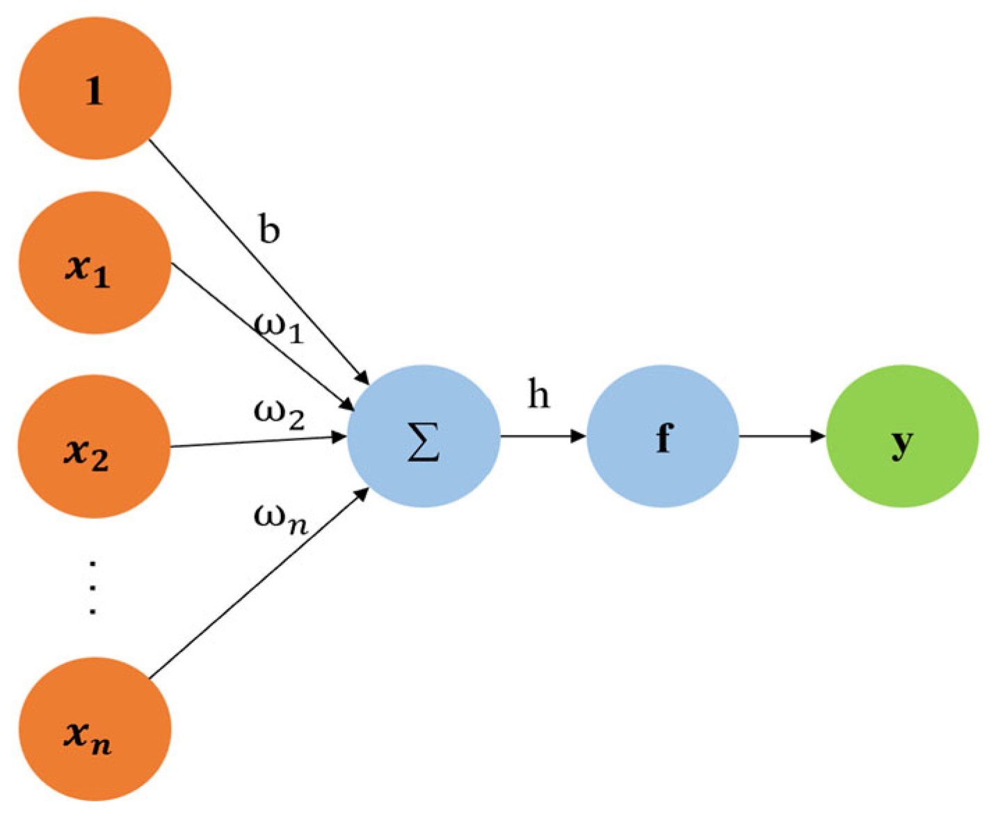
The neuron is the basic unit of a neural network, as shown in Figure 1. It mainly uses the knowledge of bionics to simulate the structure and characteristics of biological neurons, and receives and processes a group of input signals to produce output. The linear output component is expressed as Equation (26).

$$h=\sum _{i=1}^n{\omega }_i{x}_i+b$$

(26)

The vector $\left(x_1,x_2,\dots ,x_n\right)$ represents the input of the neuron, $\left({\omega }_1,{\omega }_2,\dots ,{\omega }_n\right)$ denotes the weight coefficient corresponding to the input, $b$ is the bias term, and $h$ stands for the linear output of the neuron. If $\mathbf{x}=(1,x_1,x_2,\dots ,x_n{)}^T$ is the input vector, $\mathbf{w}=(b,{\omega }_1,{\omega }_2,\dots ,{\omega }_n{)}^T$ is the parameter vector. Equation (26) can also be rewritten as Equation (27):

$$h={\mathbf{w}}^T\mathbf{x}$$

(27)

After the linear output is processed by the nonlinear function $f$, the final output $y$ is generated, as shown in Equation (28):

$$y=f\left(h\right)=f\left({\mathbf{w}}^T\mathbf{x}\right)$$

(28)

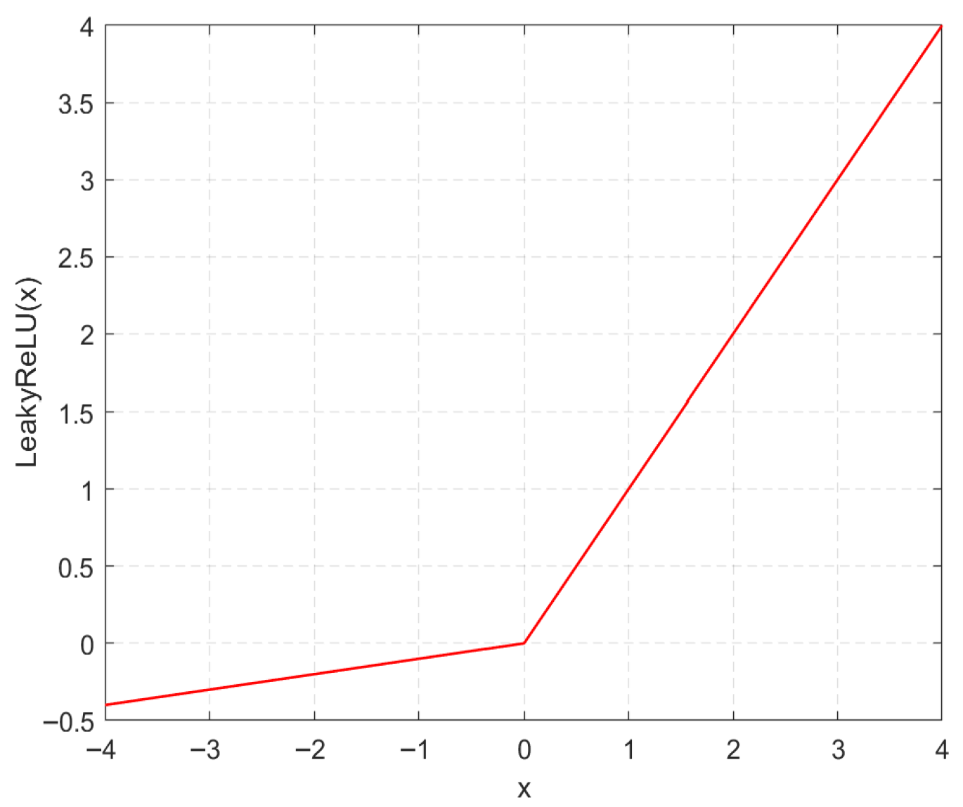
Function $f$ is called the activation function, which plays a crucial role in the operation of neurons and the overall performance of neural networks. It enables neural networks to deal with complex nonlinear problems. Simple, continuous and differentiable activation functions can typically enhance the representation and learning ability of networks. Commonly used activation functions include Sigmoid, Tanh, ReLU, and LeakyReLU. The fitting model in this paper uses the LeakyReLU activation function, whose expression is given in Equation (29). Figure 2 presents the corresponding function curve.

$$LeakyReLU\left(x\right)=\left\{\begin{array}{ll}x& ,x>0\\ \gamma x& ,x\le 0\end{array}\right.$$

(29)

The LeakyReLU activation function is a ReLU function with leakage. It is an improved version of the ReLU function. It not only inherits the advantages of the standard ReLU function—simplicity, computational efficiency, and gradient vanishing mitigation—but also resolves the neuron death problem associated with ReLU by introducing a leakage coefficient $\gamma$ (typically set to 0.01).

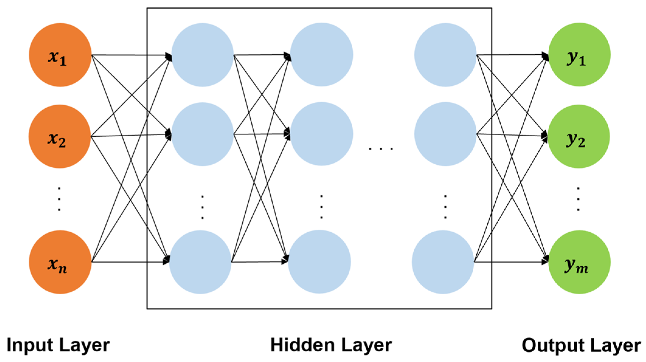
Multiple neurons can be interconnected in a specific architecture to form a multilayer feedforward perceptron (MLP). As shown in Figure 3, an MLP is composed of an input layer, an output layer, and several hidden layers. Adjacent layers are fully connected, and the output of the previous layer is used as the input of the next layer. The number of neurons in the input and output layers of an MLP network is determined by the input and output characteristics of the machine learning database. In contrast to the fixed structure of the input and output layers, the number of hidden layers and the number of neurons in each layer are hyperparameters that can be adjusted manually. A larger number of hidden layers and neurons per layer can make it easier to learn the deep-seated features in the input data, but it will also increase the complexity and training difficulty of the model, so it is necessary to select the appropriate hidden layer architecture.

2.3.2. KAN

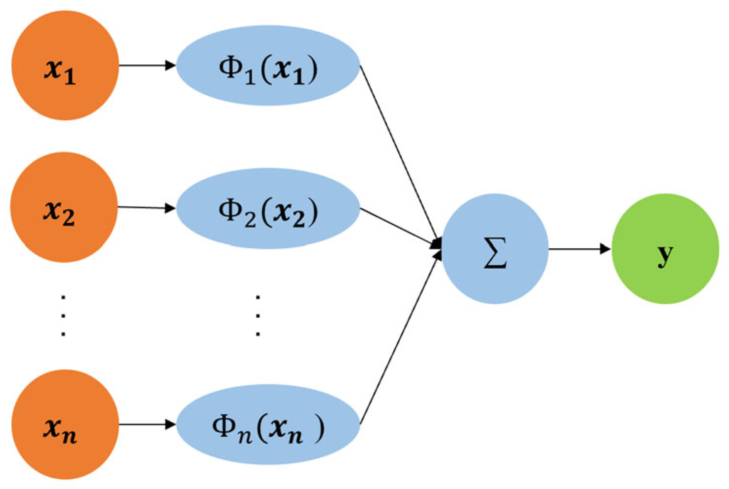
In the MLP model, the activation function is fixed and placed in neurons, while the learnable weights and biases are assigned to the edge connecting two adjacent layers of neurons. Unlike the MLP, the KAN places the learnable activation function on the edge connecting two adjacent neurons, and the model learns the parameters in each activation function. Its neuron structure is shown in Figure 4.

It can be expressed as

$$y=\sum _{i=1}^n{\varphi }_i\left(x_i\right)$$

(30)

where $\varphi \left(x\right)$ is a learnable activation function

$$\varphi \left(x\right)={\omega }_{b}b\left(x\right)+{\omega }_{s}spline\left(x\right)$$

(31)

$b\left(x\right)$ is a basis function analogous to the residual connection, which is typically configured as the SiLU function (Sigmoid Linear Unit)

$$b\left(x\right)=silu\left(x\right)={\displaystyle \frac{x}{1+e^{-x}}}$$

(32)

$spline\left(x\right)$ is a spline curve and a linear combination of B-splines

$$spline\left(x\right)=\sum _{i=0}^k{c}_i{B}_i\left(x\right)$$

(33)

$B_i\left(x\right)$ is a B-spline basis function, and $c_i$ is a trainable coefficient. The shape of the spline function can be flexibly controlled by adjusting $c_i$. The parameters ${\omega }_b$ and ${\omega }_s$ in Equation (31) are also trainable weights, which are used to adjust the contribution ratio of the basis function $b\left(x\right)$ and spline function $spline\left(x\right)$. Thus, in a KAN neuron structure, the trainable parameters can be expressed as a parameter vector $\left({\omega }_b,{\omega }_s,c_0,c_1,\dots ,c_k\right)$.

Like the MLP network, the KAN is also a fully connected network. Neurons between adjacent layers are fully interconnected to form a network structure. Similarly to the MLP, the KAN is also composed of an input layer, several hidden layers, and an output layer. The fundamental difference between the two stems from their neuron structures. Although both networks learn parameters on the edges, the MLP directly optimizes the weights and biases assigned to the edges, whereas the KAN learns the activation functions on the edges—specifically, the trainable parameters embedded within these activation functions.

2.3.3. Learning Process

For a well-constructed network model, optimizing the network parameters to achieve a good fit with the dataset is the learning process of the neural network, which is implemented via the error backpropagation (BP) algorithm. The BP algorithm mainly comprises four steps: forward propagation, loss calculation, backpropagation, and parameter update. The forward propagation process of the neural network is analogous to the neuron calculation process, as expressed in Equation (28). The predicted value of the network can be calculated through the forward propagation of the input data. The predicted value and the actual output value are not exactly the same, and there is an error between them. This error is a function of the parameters of the neural network, which is called the loss function. Neural networks designed for function fitting tasks typically adopt the mean square error (MSE) loss function. In this paper, the weighted mean square error (WMSE) is used, which can distinguish the importance of different samples through the weight coefficient to effectively suppress the influence of outliers, as expressed in Equation (34):

$$J\left(\mathbf{w}\right)={\displaystyle \frac{1}{\sum _{i=1}^m{\alpha }_i}}\sum _{i=1}^m{\alpha }_i{\left({\widehat{y}}_i-y_i\right)}^2$$

(34)

where $J\left(\mathbf{w}\right)$ is the loss function; $\mathbf{w}$ is the parameter vector corresponding to the weight coefficient and bias term in the MLP model and the parameter in the activation function in the KAN model; ${\alpha }_i$ is the weight of the ith output; ${\widehat{y}}_i$ is the predictive value of the neural network; and $y_i$ is the actual target value. The learning process of the neural network aims to find the optimal parameter vector $\mathbf{w}$ and minimize the loss function as much as possible.

If ${\mathbf{w}}^{\ast }$ is used to denote the optimal parameters obtained from neural network training, the optimization problem of neural network can be expressed as Equation (35):

$${\mathbf{w}}^{\ast }=\underset{\mathbf{w}}{\mathrm{a}\mathrm{r}\mathrm{g}\mathrm{m}\mathrm{i}\mathrm{n}}J\left(\mathbf{w}\right)$$

(35)

The gradient descent method can efficiently find the optimal parameter ${\mathbf{w}}^{\ast }$ of the model, so as to solve the optimization problem described by the aforementioned formula. Common gradient descent methods include batch gradient descent (BGD) and stochastic gradient descent (SGD), but these algorithms are only effective for the loss function which is convex (there is only a minimum in the training range). For non-convex loss functions, these methods may converge to local optimal solutions. Thus, improved algorithms such as Momentum, Adagrad, Adam, and AdamW have been proposed. This paper uses the Adam and AdamW optimizers. Regardless of the type of optimization algorithm adopted, calculating the gradient of the loss function is the key to training a network. According to the chain rule of differentiation, the error term of the preceding layer can be calculated by the error term of the subsequent layer, which is the backpropagation process of the error. Every time the error term of a layer is calculated, the parameter values can be updated based on the value of the error term and the learning rate, which corresponds to the parameter update phase. Finally, the optimal parameter ${\mathbf{w}}^{\ast }$ is obtained through multiple rounds of epoch-based iterative training, thus solving the optimization problem presented in Equation (35).

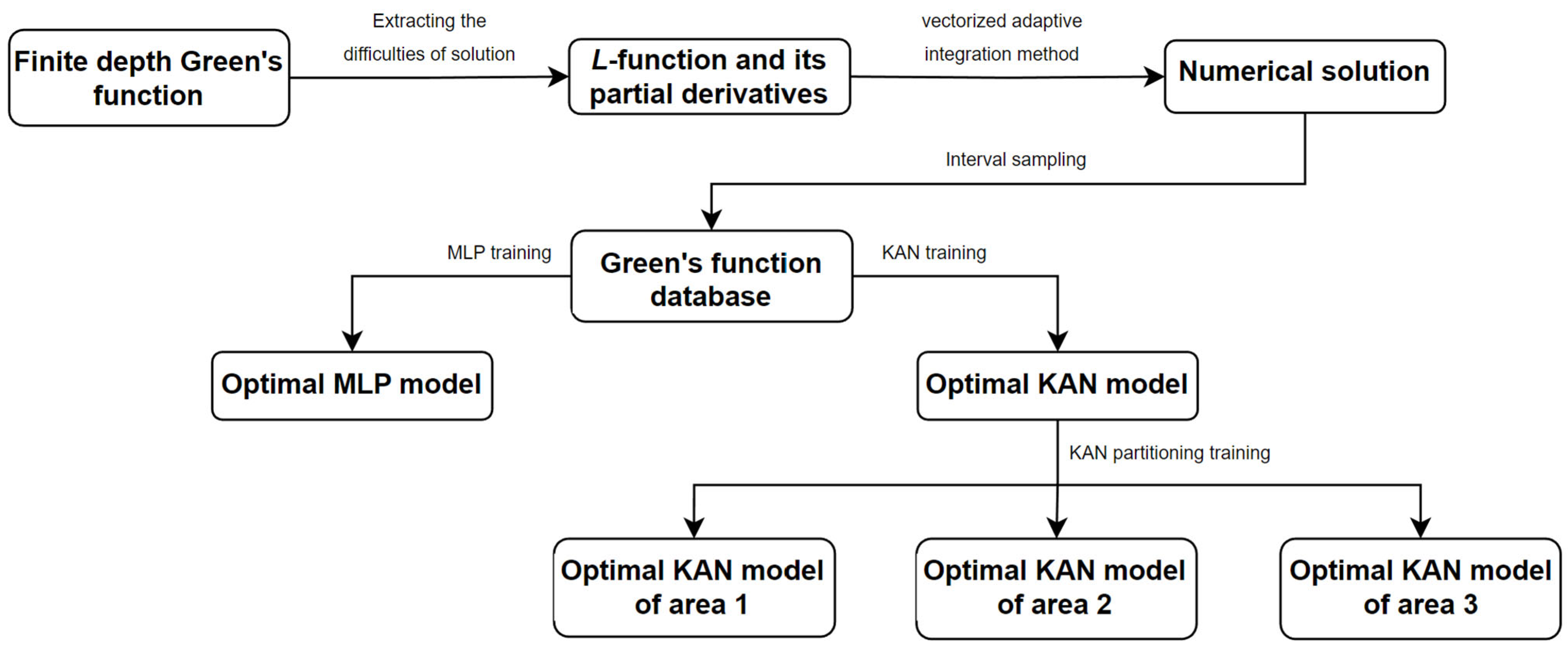
The flowchart of the entire method is shown in Figure 5. Firstly, the solution difficulties from the expression of the finite depth Green’s function are extracted, namely the L-function and its partial derivatives. Then, the numerical solutions of these functions are obtained through MATLAB’s (MATLAB R2022a, The MathWorks, Inc., Natick, MA, USA) vectorized adaptive integration method. Next, interval sampling is used to obtain the Green’s function database for neural network training. In terms of neural networks, the classic MLP network and the emerging KAN were selected, and the optimal network models were trained separately. In order to further improve the fitting accuracy of the network, considering the excellent performance of the KAN, partition fitting training was carried out on the KAN, and the optimal network models for the three partitions were obtained.

3. Experiment

Since $L\left(A,B_1,B_2,H\right)$, ${\displaystyle \frac{\partial L}{\partial A}}$, ${\displaystyle \frac{\partial L}{\partial B_1}}$, and ${\displaystyle \frac{\partial L}{\partial B_2}}$ are all four-input-one-output functions, in order to fit these functions, four four-input-one-output neural network models need to be constructed. Following the completion of global fitting, a partitioned fitting approach is further adopted in subsequent steps to enhance the fitting accuracy, yielding a remarkable improvement effect. The experiments in this paper focus primarily on the $L\left(A,B_1,B_2,H\right)$ function; the same methodology can be applied to the other three functions.

3.1. Finite Depth Green’s Function Database

The values of functions $L$, ${\displaystyle \frac{\partial L}{\partial A}}$, ${\displaystyle \frac{\partial L}{\partial B_1}}$, and ${\displaystyle \frac{\partial L}{\partial B_2}}$ are obtained by the numerical integration method. A selection of random numerical calculation results for these functions is presented in

Table 1. Numerical calculation results of target functions.

Function	(0.1,0.2,0.3,0.4)	(0.5,0.4,0.6,1.5)	(0.5,0.5,1.5,2.0)	(0.8,0.6,1.2,3.0)
$L$	−2.896232652071353	−4.554281368674081	−5.828718140182938	−5.099429117515967
${\displaystyle \frac{\partial L}{\partial A}}$	0.000742349328632	0.639683290640316	−2.005721462622466	2.957286312875203
${\displaystyle \frac{\partial L}{\partial B_1}}$	0.069554085250857	−0.294880947682861	−0.659430838361346	−0.815289410175877
${\displaystyle \frac{\partial L}{\partial B_2}}$	0.106809704551687	−0.413385067306579	−1.231124573891669	−3.041768331134250

.

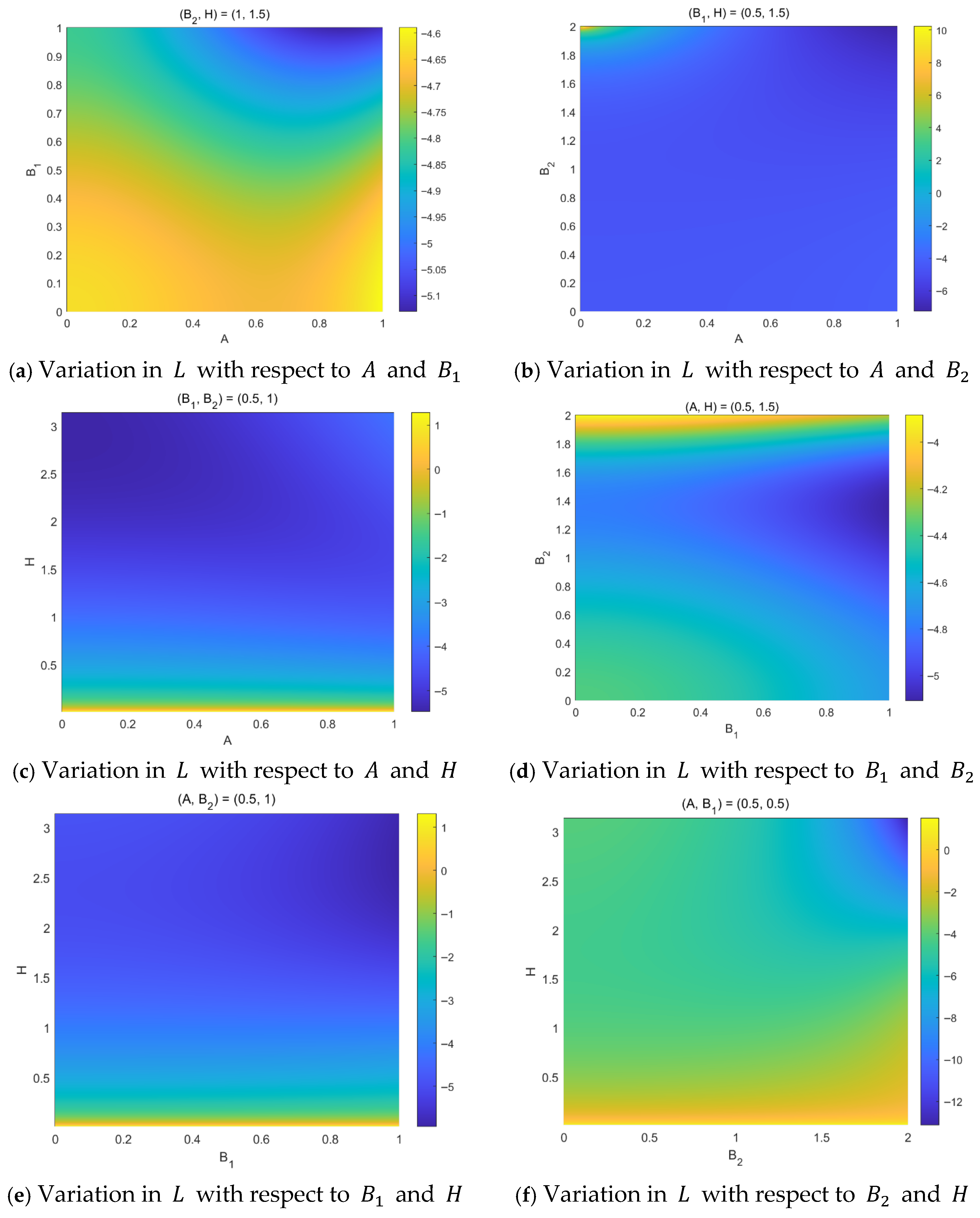
To visualize the relationship between the function and its variables, two variables can be fixed while observing the variation in the function with respect to the remaining two variables. The visualization result for the L function is presented in Figure 6.

By sampling the function $L$ over the interval of $\left[0,1\right] \times \left[0,1\right] \times \left[0,2\right] \times \left[0,\pi \right]$, the database required for machine learning can be obtained. As can be seen from Figure 6, the variation in L along the A direction is minor, whereas the function is sensitive to changes in $B_1$, $B_2,$ and $H$. Therefore, when sampling, the sampling density in the $A$ direction can be appropriately reduced, while the number of samples in the other three directions can be increased. The final sampling resolution is $0.05 \times 0.02 \times 0.02 \times 0.02$.

For the aforementioned database, two distinct fitting schemes can be designed. The first is global fitting, which involves constructing a neural network to fit the entire dataset. Given the strong fitting capability of neural networks, this scheme is feasible. In view of the heterogeneous variations exhibited by the target function across different subdomains of the defined interval, a partitioned fitting scheme can be adopted to achieve superior fitting performance. Specifically, the fitting interval is divided into several subdomains according to the variation characteristics of the function, and a dedicated neural network model is established for each subdomain to conduct localized fitting, thereby improving the overall fitting accuracy.

3.2. Global Fitting Results and Accuracy Analysis

3.2.1. MLP Model

The selection ranges of the number of hidden layers layer and the number of neurons per layer unit are [2, 3, 4, 5, 6, 7] and [256, 512, 1024, 2048, 4096], respectively. Different neural network architectures are combined and trained under different batch sizes. The selection range of batch size is [256, 512, 1024, 2048]. Finally, WMSE loss tables corresponding to different network architectures trained with different batch sizes were obtained.

Table 2. WMSE training loss results of the L function under different batch sizes.

Batch size = 256
	Unit	256	512	1024	2048	4096
Layer
2		243	171	157	125	123
3		49	29	13	9	7
4		5	6	4	6	2
5		8	4	4	6	1
6		5	4	3	4	9
7		5	3	2	4	NaN
	Batch size = 512
	Unit	256	512	1024	2048	4096
Layer
2		470	163	210	217	216
3		34	19	15	10	10
4		6	5	3	2	1
5		5	5	6	5	2
6		5	5	4	3	5
7		6	4	3	5	3
	Batch size = 1024
	Unit	256	512	1024	2048	4096
Layer
2		773	632	640	715	925
3		52	29	21	16	14
4		8	6	5	2	1
5		7	5	6	5	3
6		7	5	4	3	5
7		7	5	5	3	3
	Batch size = 2048
	Unit	256	512	1024	2048	4096
Layer
2		1047	990	1420	2200	2789
3		64	86	43	31	26
4		12	9	6	9	2
5		10	8	5	4	2
6		11	9	6	5	3
7		11	9	7	4	4

shows the training results of $L$ function, and the unit of loss is 1 × 10⁻⁶.

During the training process, it can be obviously seen that a larger batch size corresponds to a faster training speed. However, as indicated in Table 2, when the network architecture is fixed, a larger batch size generally leads to a decrease in training accuracy. Therefore, selecting an appropriate batch size can improve the training speed and obtain satisfactory training accuracy at the same time. Based on the experimental results, and considering both training speed and accuracy, a batch size of 512 was ultimately selected. As can be seen from the results in Table 2, the 4 × 4096 network (i.e., 4 hidden layers with 4096 neurons per layer) under the condition of Batch size = 512 yields the optimal fitting accuracy and is thus identified as the best-performing MLP model. In order to quantify the fitting accuracy of the model, the negative logarithm E of the absolute error can be adopted for characterization, as expressed in Equation (36):

$$E=-lg\left|\widehat{y}-y\right|$$

(36)

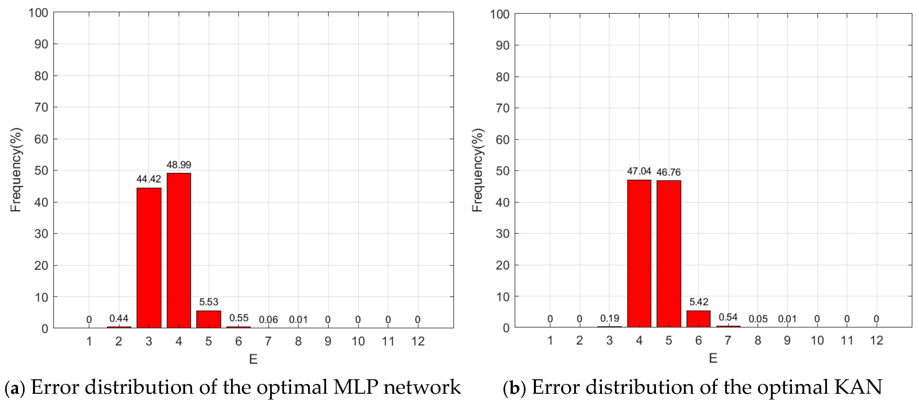
The optimal MLP model E distribution is shown in Figure 7a.

In Figure 7, an abscissa value of 3 indicates that the fitting error falls within the range of ${10}^{-2}\sim {10}^{-3}$, and so forth. When the error E of the Green function fitting is small, the subsequent hydrodynamic parameters (e.g., added mass, damping coefficients, excitation forces) calculated based on this function will have higher precision. This ensures that the numerical simulation results of the structural dynamic response are more consistent with the actual physical process. Conversely, a large E will introduce cumulative errors into the hydrodynamic calculation chain, leading to deviations between the predicted structural performance (e.g., motion response amplitude operators, RAOs) and the real situation, which may affect the reliability of offshore structure design and safety evaluation. As can be seen from Figure 7a, the fitting error of the optimal MLP model exceeds ${10}^{-3}$ for 44.86% of the samples, while only 55.14% of the samples achieve 3D fitting accuracy, which is difficult to meet the requirements of hydrodynamic calculations. Therefore, subsequent research efforts should focus on the KAN model.

3.2.2. KAN Model

The experimental setup for the KAN model is consistent with that of the MLP model. Specifically, different network architectures were constructed by varying the number of hidden layers and the number of neurons per layer, and the corresponding results under different batch sizes were obtained. The experimental results are presented directly herein. The optimal KAN model corresponds to a 2 × 128 network (i.e., 2 hidden layers with 128 neurons per layer), trained with a batch size of 128.

Table 3. The structural and training details of the optimal MLP network and KANs.

Network	Structure	Training Batch Size	Optimizer	Learning Rate	Loss Function	Activation Function	Training Time
MLP	4 × 4096 × 4096 × 4096 × 4096 × 1	512	Adam	0.001	WMSE	LeakyReLU	About 4.5 h
KAN	4 × 128 × 128 × 1	128	AdamW	0.001	WMSE	LeakyReLU	About 19 h

summarizes the structural and training details of both the optimal MLP and KANs. The distribution of the fitting error E is illustrated in Figure 7b.

Comparing Figure 7a,b, it can be seen that the fitting performance of the KAN is significantly superior to that of the MLP network. Specifically, the fitting error of 98.81% of the data samples is less than ${10}^{-3}$, while the fitting error of 54.39% of the samples is less than ${10}^{-4}$, which fully satisfies the accuracy requirements of hydrodynamic calculations. Some random fitting results of the KAN model for $L$ function are presented in the table below.

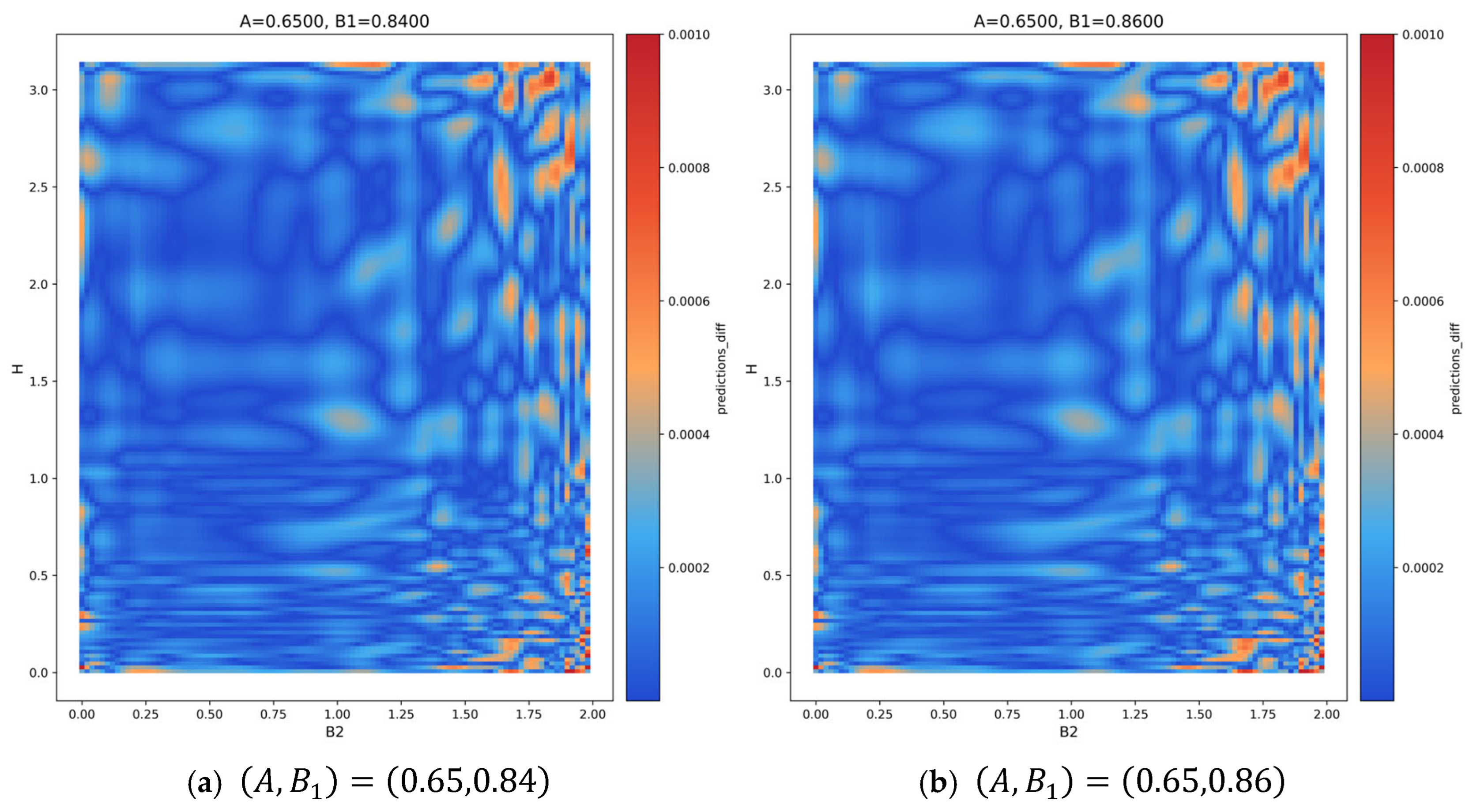
Figure 8 presents the global fitting error distribution with poor fitting performance. As illustrated in the figure, the high-magnitude errors are primarily concentrated in the edge regions of the function domain, and their proportion is relatively small within the overall distribution. Thus, the overall average error still satisfies the accuracy requirements for hydrodynamic fitting tasks.

3.3. Partition Fitting Results and Accuracy Analysis

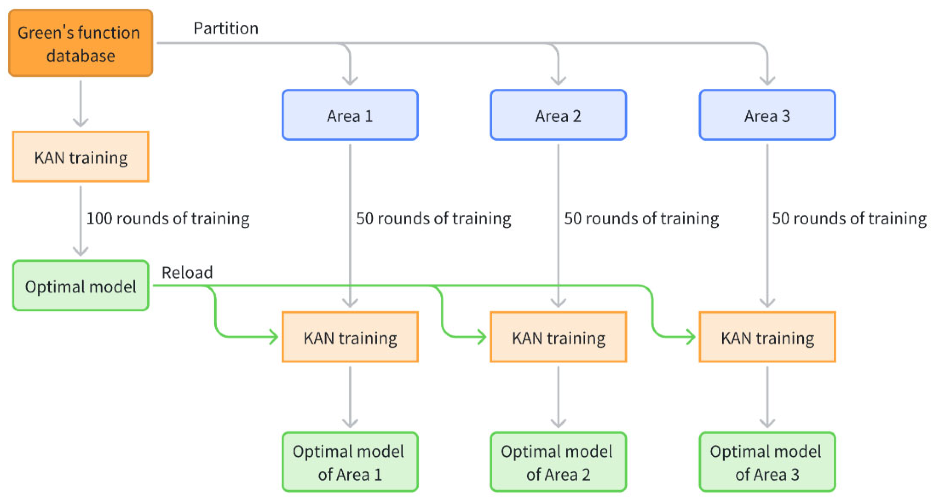
Analysis of the global fitting results demonstrates that the performance of the KAN model is significantly superior to that of the MLP model. Therefore, in order to achieve the optimal fitting effect, the partition-based experiment focuses on the partition results of the KAN model. As illustrated in Figure 9, in the partition experiments, the optimal global fitting model of the KAN is adopted as a pre-trained model; this model is then fine-tuned and retrained on different subdomains to derive the final model parameters corresponding to each subdomain.

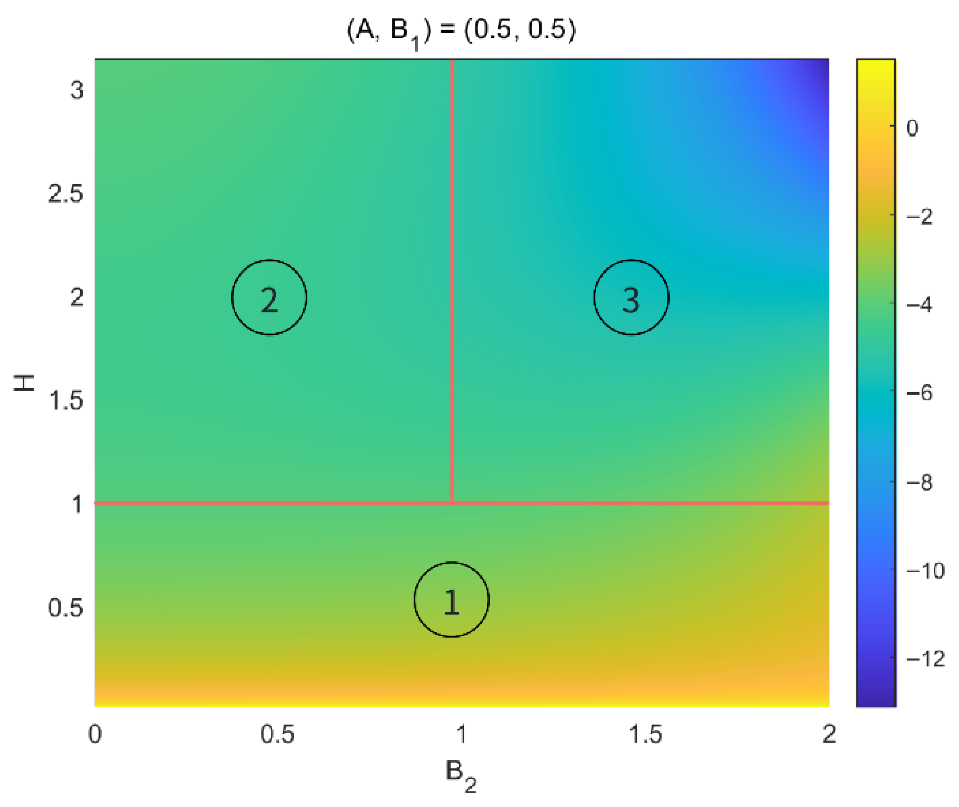
The partitioning strategy is derived from Equations (12), (13) and (15). Several functions associated with $L$ are piecewise functions, with $B_2=1$ and $H=1$ serving as the partition points. Therefore, for the purpose of partitioning, $B_2$ and $H$ axes are adopted as the partitioning criteria, and the partition boundaries are also designated as $B_2=1$ and $H=1$. For further details regarding the partitioning scheme, refer to the heatmap of the function variation with respect to $B_2$ and $H$, presented in Figure 6f; the final partitioning results are illustrated in Figure 10.

• Region 1: $H\le 1$. The function in this region exhibits significant variation with $H$.
• Region 2: $1<H$ and $B_2\le 1$. The function in this region varies gently.
• Region 3: $1<H$ and $B_2>1$. The function in this region varies with both $B_2$ and $H$, and exhibits severe mutations.

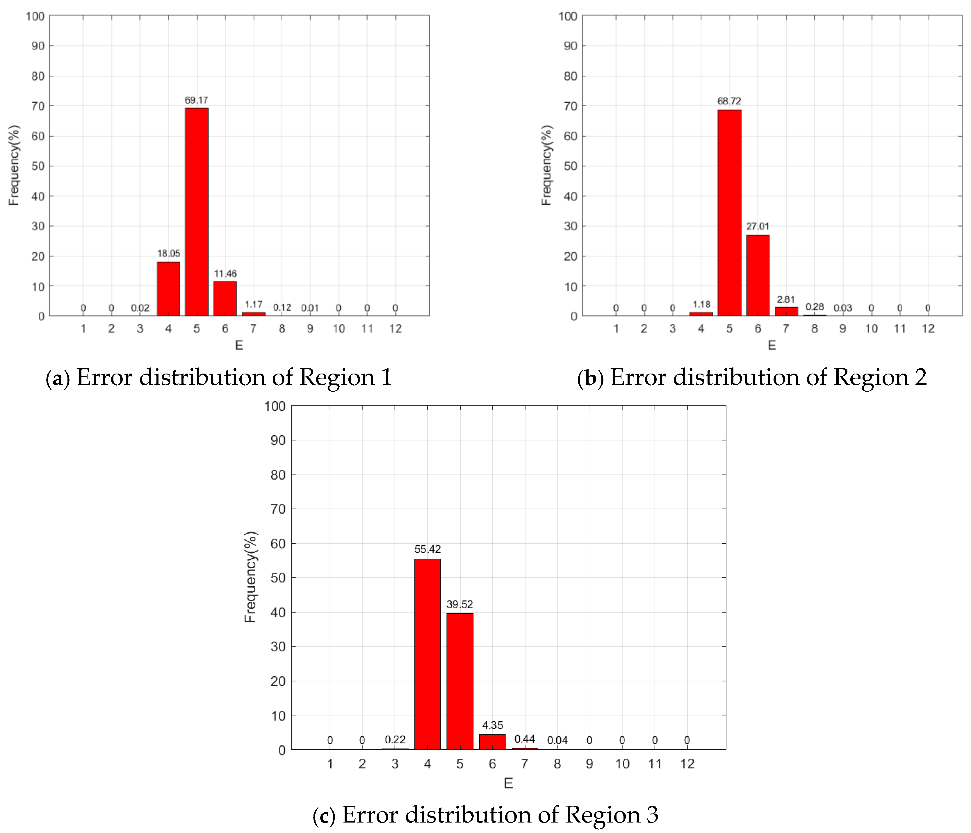
After training the KAN model in accordance with the aforementioned partitioning criteria, the optimal models for each of the three regions were obtained. The distribution of fitting error E for these region-specific optimal models is illustrated in Figure 11.

Compared with the global fitting error distribution of the KAN (Figure 7b), the partition-based fitting does not yield a significant improvement in Region 3. However, the improvement effect is remarkably obvious in Regions 1 and 2, with Region 2 achieving a 4D fitting accuracy. Consequently, the partition-based fitting can significantly enhance the overall fitting accuracy of the model and exhibits high practicality in hydrodynamic calculation tasks.

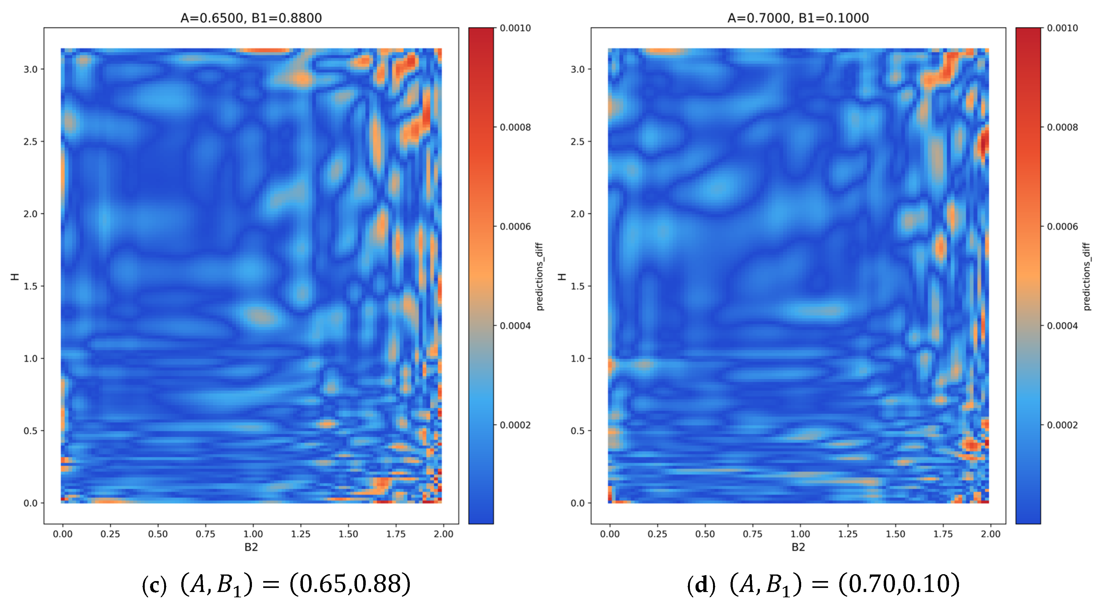
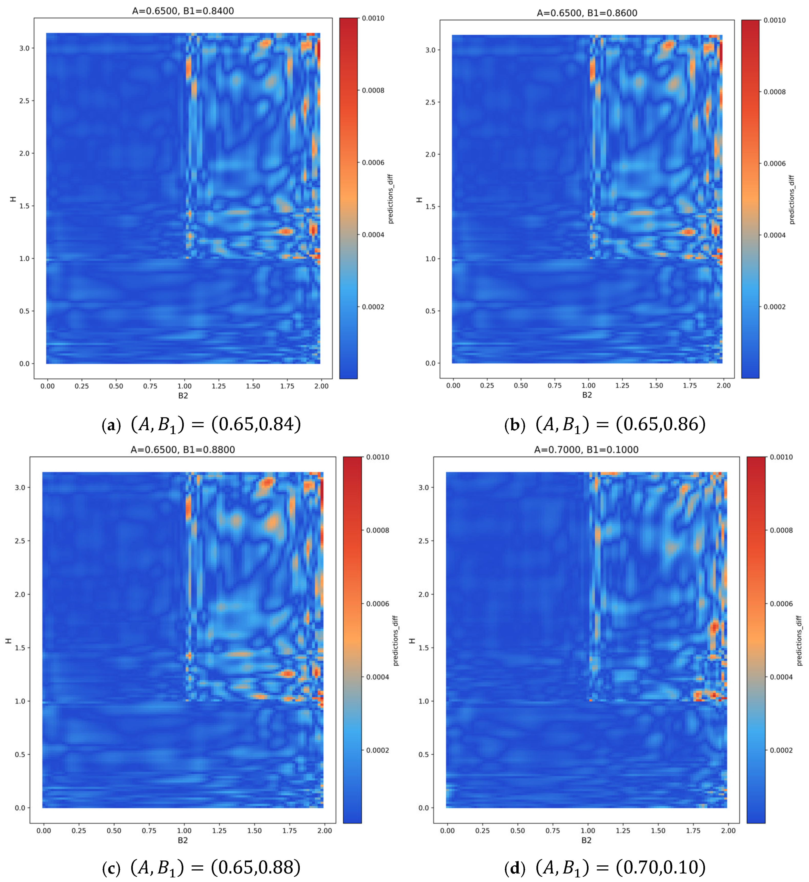
Figure 12 presents the fitting error distribution of the partitioning KAN model with poor performance, where the errors are mainly concentrated in Region 3. By comparing this with the global fitting error distribution (Figure 8), it is evident that the partition-based fitting achieves a significant improvement in Regions 1 and 2.

Table 4. Fitting results of the KAN for the L function in Region 1.

($\mathit{A},{\mathit{B}}_1,{\mathit{B}}_2,\mathit{H}$)	Numerical Integration	Global Network	Partition Network
(0.16,0.29,0.23,0.17)	−1.838383029312704	−1.8384981426522051	−1.8386414686038446
(0.28,0.35,0.29,0.23)	−2.198424101624369	−2.198387526804279	−2.1984284931483544
(0.56,0.69,1.42,0.68)	−3.236531587323570	−3.2366800407941554	−3.2364886147737155
(0.91,0.81,1.79,0.74)	−3.679273028369350	−3.679047328022239	−3.679386434746063

,

Table 5. Fitting results of the KAN for the L function in Region 2.

($\mathit{A},{\mathit{B}}_1,{\mathit{B}}_2,\mathit{H}$)	Numerical Integration	Global Network	Partition Network
(0.16,0.29,0.11,1.16)	−4.259911425363899	−4.260026655869749	−4.259931535199571
(0.28,0.35,0.26,2.27)	−4.501193534114950	−4.501101174844334	−4.501191454725541
(0.56,0.69,0.59,2.56)	−4.734606949000126	−4.734626447766143	−4.73461186618228
(0.91,0.81,0.71,3.01)	−4.136554466056646	−4.136483166155066	−4.136476467697749

and

Table 6. Fitting results of the KAN for the L function in Region 3.

($\mathit{A},{\mathit{B}}_1,{\mathit{B}}_2,\mathit{H}$)	Numerical Integration	Global Network	Partition Network
(0.16,0.29,1.17,1.16)	−4.151720618549937	−4.152152145068909	−4.151829529282919
(0.28,0.35,1.38,2.27)	−5.711437492984219	−5.711517685792271	−5.711353415343703
(0.56,0.69,1.74,2.56)	−8.195010939627185	−8.195085650282254	−8.19494851233476
(0.91,0.81,1.89,3.01)	−10.021807190363528	−10.02216359434432	−10.021408492555896

present the numerical integration results, global fitting results, and partition-based fitting results corresponding to several randomly selected input values. Both the global results and the partition-based results achieved 3D accuracy at least, while certain partition-based fitting results reached 4D accuracy. These findings verify the effectiveness and practicality of the partition-based fitting model.

3.4. Computational Efficiency Analysis

The efficiency of the proposed partition-based KAN fitting model was evaluated on a personal computer (PC) equipped with an Intel Core i5-13400F CPU (Intel Corporation, Santa Clara, CA, USA) and an NVIDIA RTX 4070 GPU (NVIDIA Corporation, Santa Clara, CA, USA). The detailed efficiency evaluation results are presented in

Table 7. Efficiency performance of the partition-based KAN fitting model.

Sampling Density	CPU	GPU	Total Time (s)	Average Time (μs)
$0.05\times 0.02\times 0.02\times 0.02$	i5-13400F	RTX4070	1.46	0.0868

.

The efficiency evaluation was conducted over the entire function domain $\left[0,1\right] \times \left[0,1\right] \times \left[0,2\right] \times \left[0,\pi \right]$, with a sampling density of $0.05 \times 0.02 \times 0.02 \times 0.02$, resulting in a total of approximately 16 million input data. The total computation time of processing all data is 1.46 s, corresponding to an average evaluation time of about 0.0868 microseconds per input; this is significantly faster than the traditional numerical integration method, which requires 0.1120 s per calculation. When the BEM program is used to calculate the hydrodynamic performance of large offshore structures, the computational scale of Green’s function reaches approximately $5\times {10}^7$ evaluations. Employing the KAN model for all Green’s function evaluations yields a total computation time of about 4.34 s, demonstrating that the model’s computational efficiency fully meets the requirements of practical engineering calculations.

4. Conclusions

In this paper, a fast-fitting method of finite-depth Green’s function using a machine learning neural network is proposed. The key challenge in solving the integral expression of the finite-depth Green’s function lies in the principal value integral component. Based on Mackay’s research, the expressions of functions $L$, ${\displaystyle \frac{\partial L}{\partial A}}$, ${\displaystyle \frac{\partial L}{\partial B_1}}$, and ${\displaystyle \frac{\partial L}{\partial B_2}}$ associated with Green’s function and its derivatives are derived in this paper, and the numerical results of these functions with 10D precision are obtained by the numerical integration method, which serve as the dataset for training the neural network. In order to fit these functions, both the classical MLP network and the emerging KAN are employed. Experiments indicate that only approximately 55.14% of the fitting results of the optimal MLP network achieve 3D accuracy, failing to meet the requirements of hydrodynamic calculations, while approximately 99.81% of the fitting results of the optimal KAN exceed 3D accuracy, with 54.39% reaching 4D accuracy, which satisfies practical engineering needs. Thus, the KAN model is ultimately adopted. To further improve the model accuracy, the original dataset is divided into three subdomains, and a dedicated KAN is established for fitting each subdomain. Experiments demonstrate that the partition-based model achieves a significant accuracy improvement in Subdomains 1 and 2, outperforming the global KAN fitting model notably. Eventually, a neural network model based on KAN is established for fitting the finite-water-depth Green’s function. Compared with traditional methods, the proposed method exhibits the following characteristics:

• Simplified implementation: The traditional polynomial fitting method relies on triple Chebyshev polynomials, involving multiple fitting functions and requiring region-specific depth fitting, leading to high implementation complexity. In contrast, the proposed method unifies multiple fitting functions into a single framework and employs neural networks for fitting, reducing the complexity of theoretical derivation and lowering implementation difficulty.
• High fitting accuracy: Most subdomains achieve 4D fitting precision. While the BEM requires 3D precision for Green’s function fitting, the proposed method meets and exceeds this requirement by achieving 4D precision in most regions, fully satisfying the demands of hydrodynamic calculations.
• Superior computational efficiency for large-scale data: Leveraging neural networks, the method can accelerate model inference via GPU acceleration, delivering higher inference efficiency under large-scale input data scenarios. Consequently, it exhibits significant computational advantages in BEM programs with extensive panel partitioning.

The machine learning neural network method holds broad application prospects in fitting free-surface Green’s functions. For the neural network-based fitting of the pulsating source Green’s function, previous studies have mainly focused on the infinite water depth scenario. This paper, for the first time, applies this method to the finite water depth condition, providing a novel solution for Green’s function fitting under such circumstances.

The work of this paper is not complete. Subsequently, we will complete the fitting of partial derivatives of the L-function and plan to develop a coupled KAN-BEM framework, where the trained KAN model directly provides Green’s function values for BEM calculations, eliminating the need for time-consuming numerical integration and further improving the computational efficiency of floating body hydrodynamic response prediction.

References

1. Hess, J.L.; Smith, A.M.O. Calculation of Nonlifting Potential Flow about Arbitrary Three-Dimensional Bodies. J. Ship Res. 1964, 8, 22–24. [Google Scholar] [CrossRef] [Scilit]
2. Fang, Z.S. Source-Dipole Method for the Calculation of Hydrodynamic Forces on Large Structures. Haiyang Gongcheng Ocean Eng. 1985, 3, 4–20. [Google Scholar] [CrossRef]
3. Zhu, R.C.; Miao, G.P.; Hong, L.; Tang, K.; Gao, Y. Some comparisons on free-surface Green function calculation and application for ship hydrodynamics. J. Hydrodyn. Ser. A. 2014, 29, 469–478. [Google Scholar]
4. Newman, J.N. Double precision evaluation of the oscillatory source potential. J. Ship Res. 1984, 28, 151–154. [Google Scholar] [CrossRef] [Scilit]
5. Newman, J.N. Algorithms for the free-surface Green function. J. Eng. Math. 1985, 19, 57–67. [Google Scholar] [CrossRef] [Scilit]
6. Wang, R.S. The Numerical Approach of Three Dimensional Free-Surface Green Function and its Derivatives (Frequency Domain-Infinite Depth). J. Hydrodyn. Ser. A 1992, 7, 277–286. [Google Scholar] [CrossRef]
7. Zhou, Q.B.; Zhang, G.; Zhu, L.S. The fast calculation of free-surface wave Green function and its derivatives. Chin. J. Comput. Phys. 1999, 16, 113–120. [Google Scholar] [CrossRef]
8. Shan, P.H.; Wang, F.H.; Wu, J.M.; Zhu, R. Application of Chebyshev Polynomials to Efficient Approximation of Frequency-Domain Infinite Depth Green Function. J. Ship Mech. 2019, 23, 1425–1433. [Google Scholar]
9. Duan, W.Y.; Yu, D.H.; Shen, Y. Algorithm for infinite depth water wave Green function and its high order derivatives. J. Ship Mech. 2016, 20, 10–22. [Google Scholar] [CrossRef]
10. Wu, H.; Zhang, C.; Zhu, Y.; Li, W.; Wan, D.; Noblesse, F. A Global Approximation to the Green Function for Diffraction Radiation of Water Waves. Eur. J. Mech. B/Fluids 2017, 65, 54–64. [Google Scholar] [CrossRef] [Scilit]
11. Chang, H.Y.; Zhu, R.C.; Huang, S. Preliminary study on prediction of pulsating source Green function based on machine learning. Haiyang Gongcheng Ocean Eng. 2020, 38, 131–141. [Google Scholar] [CrossRef]
12. He, D.L.; Zhu, R.C.; Huang, S. Progressive Forecast and Application of Three-Dimensional Frequency Domain Green Function Based on Machine Learning. Chin. J. Shipbuild. 2023, 64, 73–86. [Google Scholar] [CrossRef]
13. Zhan, K.; Zhu, R.; Xu, D. A machine learning model for fast approximation of free-surface Green’s function and its application. J. Ocean Eng. Sci. 2025, 10, 521–534. [Google Scholar] [CrossRef] [Scilit]
14. John, F. On the Motion of Floating Bodies. I. Commun. Pure Appl. Math. 1949, 2, 13–57. [Google Scholar] [CrossRef] [Scilit]
15. Endo, H. Numerical Evaluation of Principal Value Integral by Gauss-Laguerre Quadrature. AIAA J. 1983, 21, 149–151. [Google Scholar] [CrossRef] [Scilit]
16. Liu, R.; Ren, H.; Li, H. An improved Gauss-Laguerre method for finite water depth Green function and its derivatives. J. Ship Mech. 2008, 12, 188–196. [Google Scholar]
17. Yang, P.; Gu, X.; Cheng, X.; Ding, J. Numerical study of 3D pulsating source Green function in finite water depth. J. Ship Mech. 2016, 20, 57–67. [Google Scholar]
18. Shan, P.; Zhu, R.; Wang, F.; Wu, J. Efficient Approximation of Free-Surface Green Function and OpenMP Parallelization in Frequency-Domain Wave–Body Interactions. J. Mar. Sci. Technol. 2019, 24, 479–489. [Google Scholar] [CrossRef] [Scilit]
19. Liu, Y.; Cong, P.; Gou, Y.; Yoshida, S.; Kashiwagi, M. Enhanced Endo’s approach for evaluating free-surface Green’s function with application to wave-structure interactions. Ocean Eng. 2020, 207, 107377. [Google Scholar] [CrossRef] [Scilit]
20. Chen, X.B. Evaluation de la fonction de Green du probleme de diffraction/radiation en profondeur d’eau finie—Une nouvelle methode rapide et precise. In Actes des 4e Journees de l’Hydrodynamique; Presses de l’École Centrale de Nantes: Nantes, France, 1993; pp. 371–384. [Google Scholar]
21. Mackay, E. Consistent Expressions for the Free-Surface Green Function in Finite Water Depth. Appl. Ocean Res. 2019, 93, 101965. [Google Scholar] [CrossRef] [Scilit]
22. Tavakoli, S.; Khojasteh, D.; Haghani, M.; Hirdaris, S. A review on the progress and research directions of ocean engineering. Ocean Eng. 2023, 272, 113617. [Google Scholar] [CrossRef] [Scilit]
23. Hornik, K.; Stinchcombe, M.; White, H. Multilayer Feedforward Networks Are Universal Approximators. Neural Netw. 1989, 2, 359–366. [Google Scholar] [CrossRef] [Scilit]
24. Liu, Z.; Wang, Y.; Vaidya, S.; Ruehle, F.; Halverson, J.; Soljacic, M.; Hou, T.Y.; Tegmark, M. Kan: Kolmogorov-Arnold Networks. In Proceedings of the International Conference on Learning Representations, Singapore, 24–28 April 2025. [Google Scholar]
25. Hinton, G.E.; Salakhutdinov, R.R. Reducing the Dimensionality of Data with Neural Networks. Science 2006, 313, 504–507. [Google Scholar] [CrossRef] [Scilit] [PubMed]
26. Tavakoli, S.; Singh, M.; Hosseinzadeh, S.; Hu, Z.; Shao, Y.; Wang, S.; Huang, L.; Grammatikopoulos, A.; Li, Y.P.; Khojasteh, D.; et al. A Review of Flexible Fluid–Structure Interactions in the Ocean: Progress, Challenges, and Future Directions. Ocean Eng. 2025, 342, 122545. [Google Scholar] [CrossRef] [Scilit]
27. Wehausen, J.V.; Laitone, E.V. Surface Waves. In Handbuch der Physik; Springer: Berlin, Germany, 1960; Volume 9, pp. 446–778. [Google Scholar]
28. Shampine, L.F. Vectorized Adaptive Quadrature in MATLAB. J. Comput. Appl. Math. 2008, 211, 131–140. [Google Scholar] [CrossRef] [Scilit]
Figure 1. Neuron model of the MLP network. (Orange denotes the input, blue denotes the intermediate process, and green denotes the output).
Jmse 14 00203 g001
Figure 2. LeakyReLU activation function.
Jmse 14 00203 g002
Figure 3. Architecture of the MLP network. (Orange denotes the input, blue denotes the intermediate process, and green denotes the output).
Jmse 14 00203 g003
Figure 4. Neuron model of the KAN. (Orange denotes the input, blue denotes the intermediate process, and green denotes the output).
Jmse 14 00203 g004
Figure 5. The flowchart of the entire methodology.
Jmse 14 00203 g005
Figure 6. Bivariate variation in the L function.
Jmse 14 00203 g006
Figure 7. Error distribution of global fitting.
Jmse 14 00203 g007
Figure 8. Global fitting error distribution with poor performance.
Jmse 14 00203 g008aJmse 14 00203 g008b
Figure 9. Flowchart of partition-based training.
Jmse 14 00203 g009
Figure 10. Partition map. (Number 1 denotes Region 1, with all other numbers following the same correspondence rule).
Jmse 14 00203 g010
Figure 11. Error distribution of KAN partition-based fitting.
Jmse 14 00203 g011
Figure 12. Partition-based fitting error distribution of KAN with poor performance.
Jmse 14 00203 g012