Article

Mooring Tendon Dynamic Tension Estimation in a 15 MW TLP-Type FOWT: A Comparison of Self-Attention, LSTM, and GRU Networks


1
Division of Mechanical Engineering, Korea Maritime & Ocean University, Busan 49112, Republic of Korea
2
Wind Energy Research Department, Korea Institute of Energy Research, Jeju 63357, Republic of Korea
*
Authors to whom correspondence should be addressed.
J. Mar. Sci. Eng. 2026, 14(18), 1745; https://doi.org/10.3390/jmse14181745 (registering DOI)
Submission received: 7 August 2026 / Revised: 10 September 2026 / Accepted: 12 September 2026 / Published: 19 September 2026
(This article belongs to the Special Issue Numerical Analysis and Modeling of Floating Structures (2nd Edition))

Abstract

Tension Leg Platform (TLP)-type Floating Offshore Wind Turbines (FOWTs) rely on continuously pre-tensioned mooring tendons, the integrity of which must be monitored to ensure safe operation. However, direct measurement of tendon tension at submerged locations is difficult in practice. This study investigates a virtual sensing approach in which the effective tension at multiple tendon points—fairlead, middle, and anchor—of a 15 MW TLP-type FOWT is estimated from responses measured at or near the free surface. Three deep learning architectures are comparatively evaluated: a Transformer-encoder-based self-attention network (EN-ATT), Long Short-Term Memory (LSTM), and Gated Recurrent Unit (GRU). Fully coupled time-domain simulations are used to generate the training and test data, and the models are assessed under both nominal and noisy input conditions across multiple noise levels. The EN-ATT achieves the highest accuracy in terms of RMSE, MAE, and the coefficient of determination under both nominal and noisy conditions. Feature gradient analysis indicates that the self-attention model exhibits greater sensitivity to longer input lags than the recurrent networks. While the EN-ATT does not consistently outperform the recurrent networks for extreme values, the results suggest that self-attention architectures are a promising direction for mooring tension monitoring of TLP-type FOWTs.

1. Introduction

Floating Offshore Wind Turbines (FOWTs) play a pivotal role in achieving carbon neutrality [1]. Among these, Tension Leg Platform (TLP)-type FOWTs offer the distinct advantage of vertical motion stability [2,3], achieved through the pre-tension in their mooring tendons [4,5]. However, this continuous pre-tension can negatively affect structural integrity, potentially leading to tendon failure via fatigue accumulation or extreme tensile loads. Therefore, continuous monitoring of mooring tendons is essential for the safe and stable operation of TLP-type FOWTs.
Traditionally, subsea line monitoring has relied on cost-prohibitive Remotely Operated Vehicles (ROVs). To overcome this, sensor-based monitoring methods have gained significant attention. Several studies have successfully demonstrated underwater line and riser monitoring frameworks using mathematical models [6,7,8,9,10]. In particular, Chung et al. [6] showed that the bending moments and tensions at the top, middle, and bottom sections of the tendon can be effectively estimated using top-tension and inclinometer sensor signals of a TLP-type FOWT.
In recent years, numerous studies have investigated offshore monitoring systems using machine learning techniques, commonly referred to as Artificial Intelligence (AI), owing to their capability to model complex nonlinear behaviors and extract hidden patterns from large amounts of monitoring data. Chung et al. [11] applied a Deep Neural Network (DNN) to detect damaged mooring lines in a TLP system. In that study, a supervised classification neural network was developed to determine whether a tendon was damaged using the hull motion responses as input features. Moreover, Lee et al. [12] developed a damage detection algorithm for catenary mooring lines with Recurrent Neural Networks (RNNs). This study was likewise formulated as a supervised classification model, and the results showed that the RNNs outperformed a conventional DNN in predictive performance.
For FOWTs, several studies have proposed monitoring algorithms based on AI. Choe et al. [13] conducted damage detection of turbine blades using Long Short-Term Memory (LSTM) and Gated Recurrent Unit (GRU) networks. This study was likewise formulated as a supervised classification task, and it was found that the GRU architecture generally exhibited superior performance compared to the other models. Moreover, Kang et al. [14] proposed an interpretable dynamic response prediction method based on attention networks.
To develop a neural-network-based model for dynamic response prediction, it is essential to conduct comparative analyses of different machine learning models to evaluate their predictive performance. In previous studies, RNNs have been predominantly employed for time-series prediction tasks [15,16,17,18,19,20]. Specifically, Min et al. [17] proposed an LSTM-based structural pattern model to estimate unmeasured structural responses, including tether tension and tunnel bending moments, of a submerged floating tunnel using readily available acceleration sensor data. Moreover, Liu and Li [19] proposed an LSTM model to predict the mechanical behavior of a lazy-wave-type dynamic power cable for an FOWT and suggested that incorporating seabed sensor data to capture buoyancy module motions could enhance prediction performance.
Recent studies indicate that self-attention-based neural networks can achieve better performance than RNNs [21,22,23,24,25,26,27]. Ye et al. [23] proposed an end-to-end convolutional neural network with an attention mechanism to predict the mooring tension responses of a semi-submersible FOWT and reported better performance compared to conventional LSTM models. They also examined feature sensitivity across input time lags to improve model interpretability; however, the resulting patterns were not related to the underlying structural dynamics. Yuan et al. [25] showed that an attention-based Transformer model achieved better time-series-based prediction of mooring tension than an LSTM model using field data from a semi-submersible platform; however, the internal learning characteristics of the model were not further investigated.
Overall, most studies have focused on semi-submersible FOWT platforms with spread mooring systems [13,14,18,19,20,21,23,24], while research on tendon monitoring in TLP systems remains relatively limited. In cases where neural networks have been applied [11], the scope has largely been confined to supervised classification tasks. For mooring tendons, although comprehensive damage assessment is important, estimating dynamic responses for time-series-based monitoring is equally critical. Consequently, the suitability of neural network architectures for predicting the dynamic tension of TLP systems, which differ significantly from semi-submersibles, has not yet been thoroughly investigated. Moreover, few studies have systematically compared neural network architectures for continuous prediction of multi-point TLP tendon tension. Therefore, this study investigates an AI-based mooring tension monitoring algorithm applicable to a TLP-type FOWT. In addition, conventional RNNs commonly used for time-series prediction—namely, LSTM and GRU—and a self-attention-based deep learning algorithm are comparatively evaluated. The major objective and contributions of this study are as follows:
  • This study focuses on estimating the dynamic mooring tension of a TLP-type FOWT, a topic that has received less attention than catenary-type FOWTs. Mooring tension was predicted using widely used RNNs (LSTM and GRU) and the self-attention-based neural network, with the three architectures comparatively evaluated.
  • The dynamic tension of the submerged tendon is predicted using only sensor information that can be easily obtained above or near the free surface.
  • For a more comprehensive evaluation, predictive performance is compared under multiple noise levels. In addition, feature gradient analysis is performed to examine and compare the structural characteristics of each neural network architecture, and to provide a physical interpretation of the models.
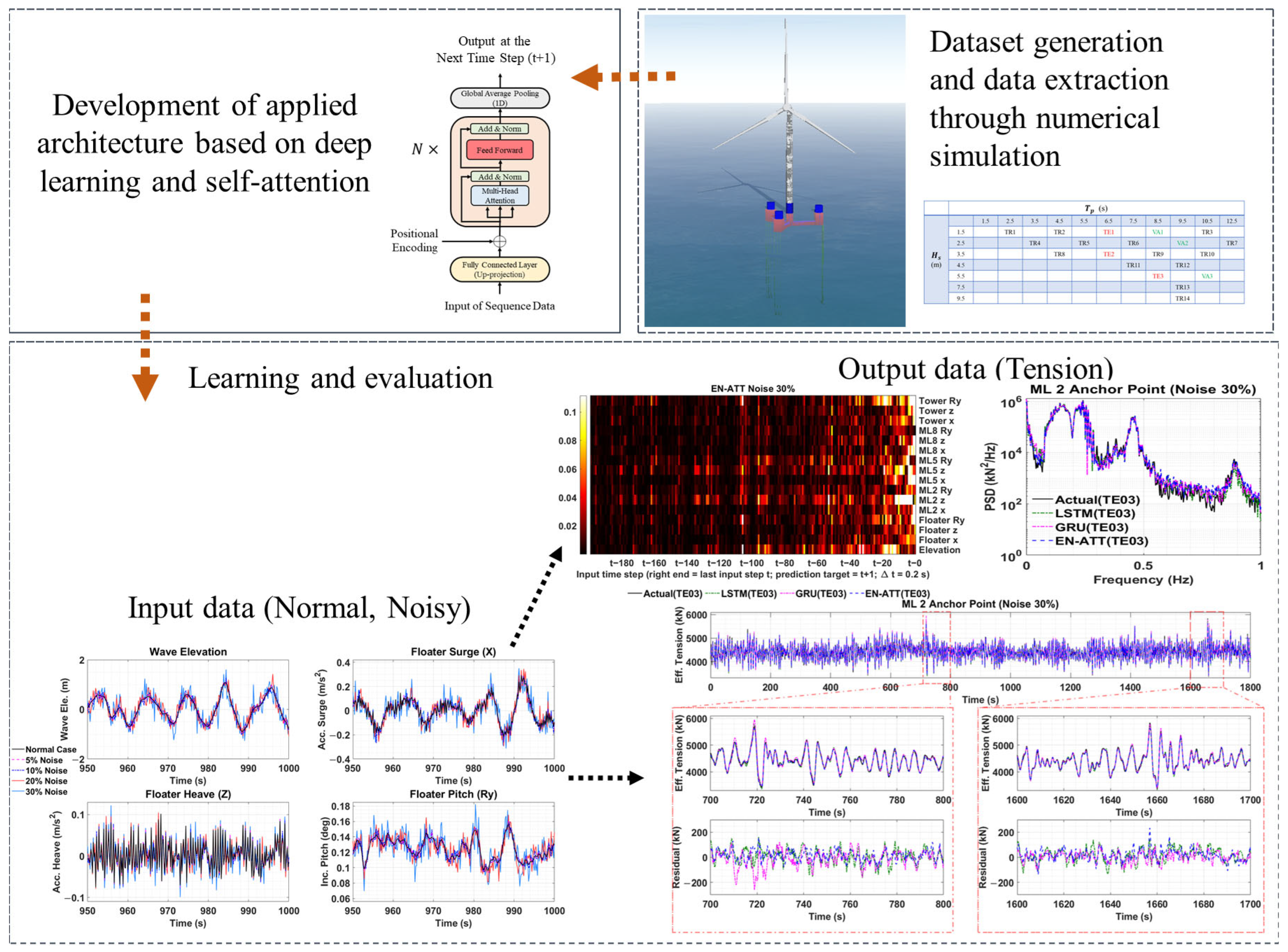
The remainder of this paper is organized as follows. Section 2 describes the FOWT system and data processing. Section 3 presents the theory and configuration of the neural networks compared in this study. Section 4 presents the results, followed by a discussion in Section 5. Section 6 outlines limitations and future research, and Section 7 concludes the paper. Figure 1 summarizes the overall workflow of this study.

2. System and Data Processing

2.1. TLP-Type FOWT System

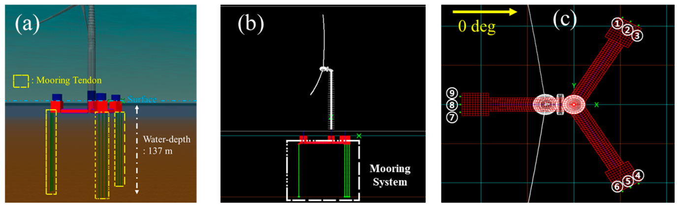
In this study, the 15 MW TLP-type FOWT is employed to explore the neural networks for mooring tension estimation. This FOWT was collaboratively developed by KRISO (Korea Research Institute of Ships and Ocean Engineering) and KIER (Korea Institute of Energy Research) [28,29]. Figure 2 presents the OrcaFlex model, the tendon numbering, and the environmental direction convention at a water depth of 137 m. The tendons are numbered clockwise from the upper-right tendon in the overview. Table 1 summarizes the principal tendon properties, while a more detailed description of the overall FOWT system is available in our previous study [30].

2.2. Case Classification by Wave Scatter Diagram

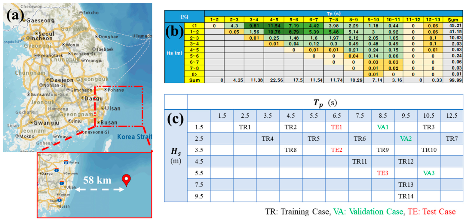
The FOWT was assumed to be installed approximately 58 km off the coast of Ulsan in the East Sea of South Korea. Figure 3a identifies the target region, and Figure 3b presents the joint distribution of significant wave height ( H s ) and peak period ( T p ) obtained from the regional wave scatter diagram [31]. Based on this distribution, 20 simulation cases were selected and assigned to the training, validation, and test sets as 14, 3, and 3 cases, respectively, as shown in Figure 3c.

2.3. Numerical Simulation for Data Generation

Numerical simulations were performed using OrcaFlex (version 11.5), a commercial dynamic analysis software for offshore marine systems [32]. All simulation scenarios employed the same wind and current speed profiles. Table 2 summarizes the environmental conditions applied to the simulation case. The wind and current conditions represented normal operating conditions, with the turbine in the power-producing state. Irregular waves and turbulent wind were generated using the JONSWAP spectrum [33] and IEC Kaimal turbulence spectrum [34], respectively. This allowed for irregular waves and turbulent wind speeds to be applied. Further details of the environmental conditions are summarized in Table 2.
The total simulation duration was 2300 s, including an initial ramp period of 500 s. Accordingly, the effective simulation time used for analysis was 1800 s. The mean environmental direction was fixed at 0° for all cases.
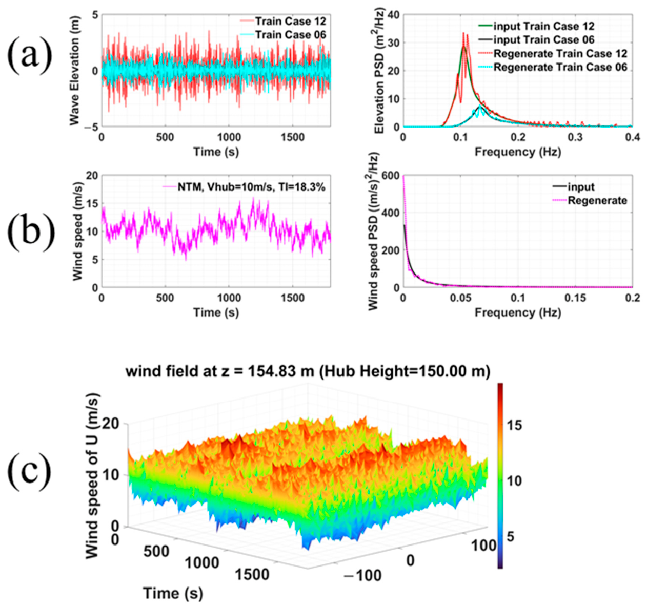
Figure 4 illustrates the wave elevation time series for training cases 6 and 12, the wind speed time series and spectra at hub-height for all cases, and the wind field of main wind direction (U) near hub-height as a time series. A comparison between the target power spectral density (PSD) and the PSD regenerated from the synthesized time series via Fast Fourier Transform (FFT) showed good agreement, confirming the reliability of the simulation time history. Furthermore, the wind field plot demonstrated that the turbulent wind speed is appropriately applied across the horizontal grid. Additionally, the coherence of the wind profile can be found in Supplementary Material S4.

2.4. Data Extraction for Training AI

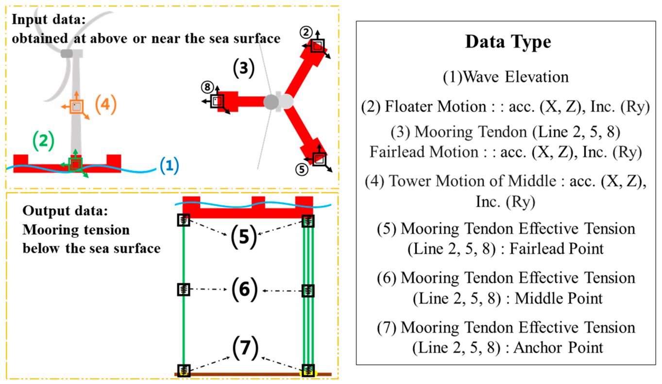
Subsequently, data were extracted from the simulation cases for training and testing the neural networks. In this study, to estimate the mooring tension time series using sensor data that can be readily obtained near the water surface, wave elevation, mooring tendon motions at the fairlead, floater motions, and tower motions were selected as input features.
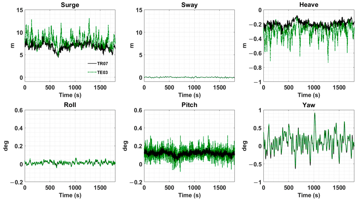
As the environmental loading direction was fixed at 0 degrees, only surge, heave, and pitch motions were considered in the analysis. The six-DOF floater responses of a representative training case (TR07) and the test case (TE03) are compared in Appendix C (Figure A2). Under this unidirectional loading, sway and roll are negligible in magnitude. As previously mentioned, this study considered a turbulent wind profile, in which case the yaw motion of the FOWT can be significantly affected by wind turbulence [35]. Because a single common wind realization was applied to all training, validation, and test cases, the yaw time history is nearly identical across cases (Figure A2), whereas the wave-dominated surge, heave, and pitch responses differ from case to case. Including yaw as an input would therefore allow the network to associate a case-independent, wind-realization-specific signal with the wind-induced tension component shared between the training and test sets; i.e., a potential source of data leakage. Yaw was thus deliberately excluded; the limitations of this choice are discussed in Section 6.
In addition, only the mooring tensions of lines #2, #5, and #8 were selected as target outputs. The selected mooring tendons were chosen as output targets because, as shown in Figure 2, they are located at the center of each tendon group and can therefore serve as representative elements of their respective groups. Additionally, similar to [6], mooring tension values were extracted at the fairlead, middle, and anchor positions of tendons #2, #5, and #8 to evaluate predictive performance at different tendon locations. Figure 5 shows the detailed configuration of the input and output data types.
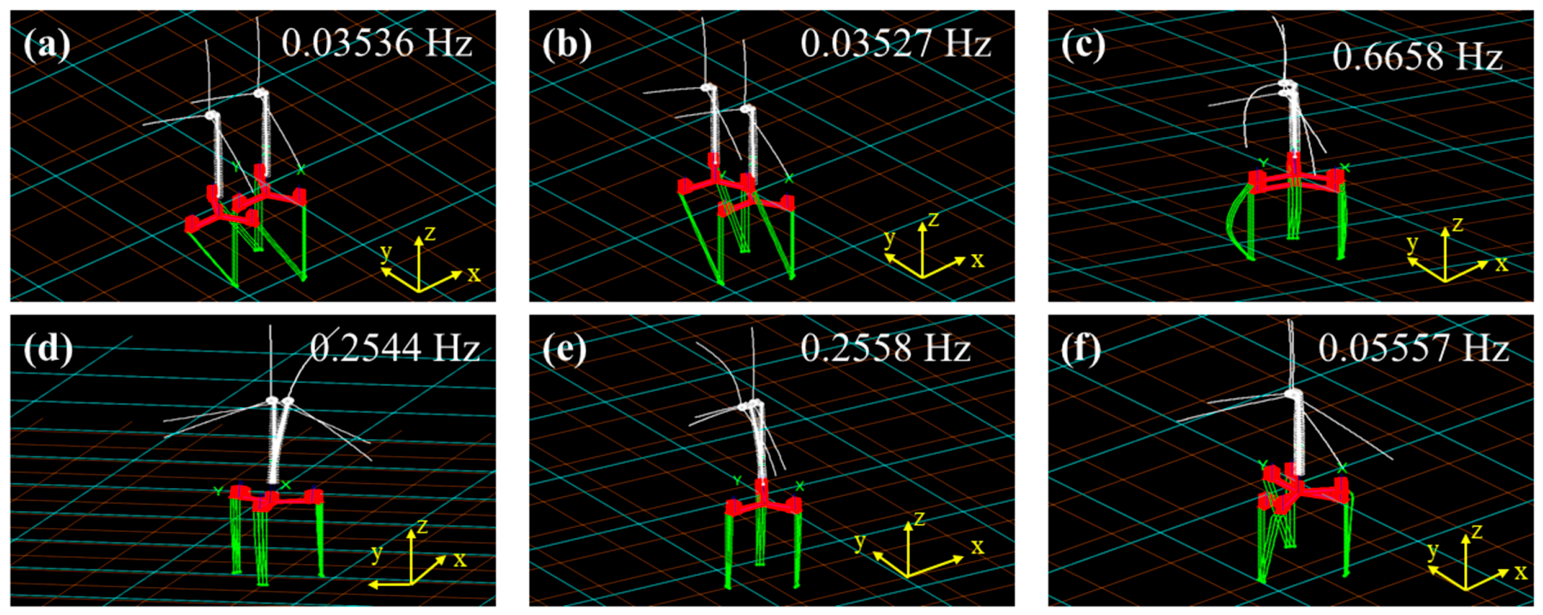
Each 1800 s analysis record contained 9001 samples at a sampling interval of 0.2 s, corresponding to a sampling frequency of 5 Hz. This sampling rate corresponds to a Nyquist frequency of 2.5 Hz [36]. The dominant global-system frequencies shown in Figure 6 lie below this limit. Because the tower and other structural components are modeled as flexible, these frequencies should not be interpreted as pure rigid-body modes. In particular, the roll- and pitch-associated responses represent coupled modes involving both floater motion and structural deformation. However, the fact that the natural frequencies of these coupled modes lie below the Nyquist limit does not by itself exclude higher-frequency components in local tendon tension; therefore, the present conclusions are restricted to the sampled bandwidth.
Table 3 summarizes the configuration of the dataset used for training, validation, and testing in this study. For continuous time-series outputs, the commonly used sliding time-window method was applied to the input vectors [14,15]. All neural networks in this study were configured in a many-to-one architecture and perform one-step-ahead prediction: an input window consisting of the 200 most recent time steps (t − 199, …, t) is used to predict the tendon tension at the next time step, t + 1, corresponding to a prediction horizon of one sampling interval (0.2 s). No synchronous (current-time) estimation is performed, and this formulation is used consistently throughout the manuscript.
The input and output window lengths were set to 200 and 1, respectively. In this context, the input window length is generally treated as a hyperparameter and therefore requires an optimization process. Details regarding this procedure are described in Section 3.4. In addition, the stride of the sliding window, which determines the window shifting interval, was set to 1 for all cases.
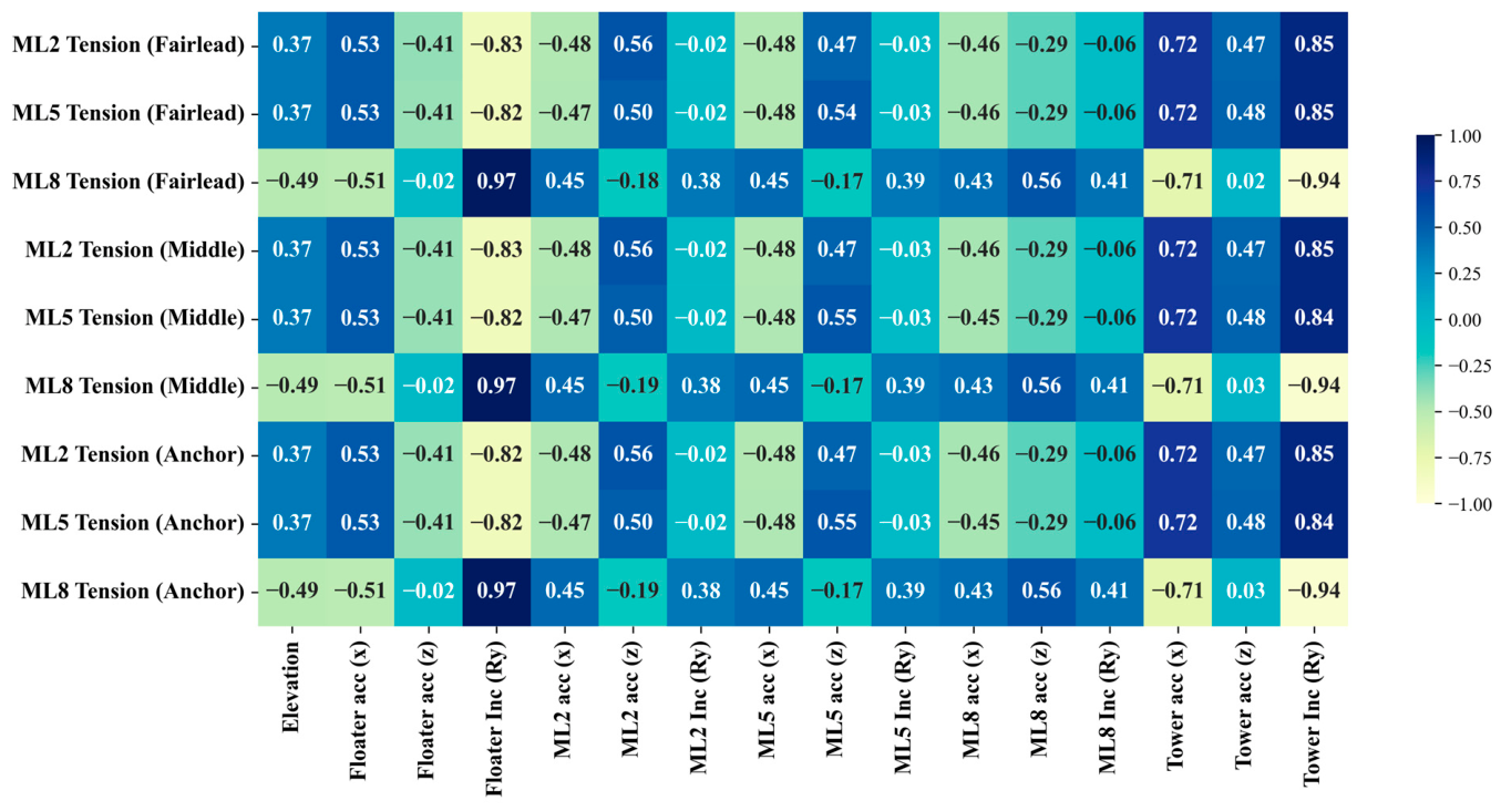
Figure 7 presents the zero-lag Pearson correlation coefficients computed from the training data. Several input–output pairs exhibited coefficients close to zero; therefore, not every input had a strong zero-lag linear association with the targets. The fairlead inclination about the global y -axis showed comparatively weak association with several, but not all, tension targets. Pearson correlation does not measure causal influence or model importance and does not capture lagged or nonlinear dependencies that may be used by the sequence models.

3. Theoretical Background and Configuration of the Neural Networks Used in This Study

3.1. LSTM and GRU

This section describes the theoretical background and configurations of the neural networks employed in this study. In this study, conventional LSTM [37] and GRU [38] networks, which are specifically designed for time-series prediction tasks, were first employed. These networks were implemented using the standard LSTM and GRU mechanisms provided as built-in functions in the TensorFlow library (version 2.10.0) in Python (version 3.8.20) [39,40]. The detailed operating principles of these architectures can be readily found in the relevant literature and previous studies [13,41].
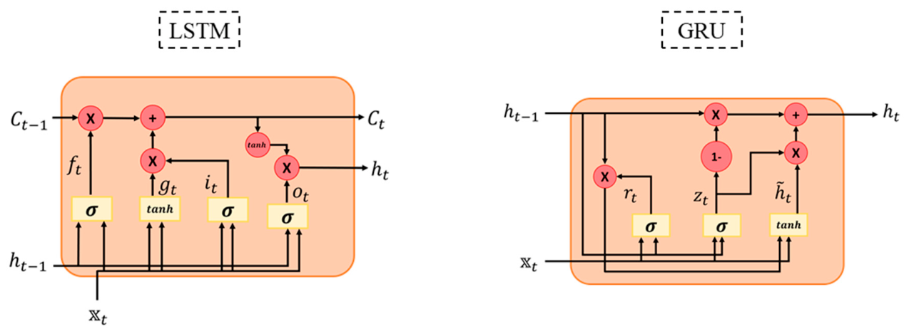
The primary difference between GRU and LSTM lies in the architectural simplicity of the GRU compared to the LSTM. This architectural distinction can be observed in Figure 8. However, despite the structural advantages of the GRU, the choice between GRU and LSTM ultimately depends on the specific task and the characteristics of the dataset [41]. Therefore, their performance is often compared empirically after training.

3.2. EN-ATT: A Transformer-Encoder-Based Self-Attention Network

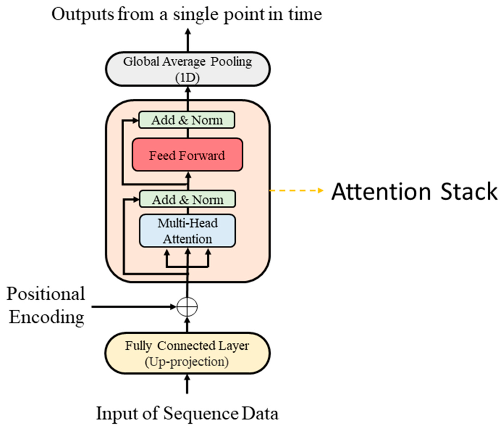
With the development of neural networks for sequential data, attention-based architectures began to emerge following the evolution of RNNs. Subsequently, with the advent of the Transformer model based on self-attention mechanisms, attention-based neural networks have become a dominant paradigm in deep learning [42]. Figure 9 illustrates the architecture of the neural network, focusing on the encoder part of the transformer model based on the self-attention mechanism adopted in this study. Hereafter, this neural network architecture is denoted as EN-ATT.
EN-ATT first receives sequential data as input, similar to traditional RNNs:
X ( n ) R t s × F
where X ( n ) denotes the standardized multivariate time-series input matrix for the n -th sample, t s denotes the sequence length (i.e., the number of time steps), and F represents the number of sensor features. However, when the number of input features (types of input data) is small, effective learning during the multi-head attention process may not be achieved. Therefore, a dense layer, similar to a hidden layer in a Multi-Layer Perceptron (MLP) neural network, was fully connected at the beginning to enrich the representation of the input features:
H n = X n W p r o j + b p r o j
H ( n ) R t s × d m o d e l
W p r o j R F × d m o d e l
where H ( n ) denotes the projected embedding matrix of the n -th sample, obtained by linearly transforming the input X n , W p r o j represents the learnable projection weight matrix, b p r o j denotes the corresponding bias vector, and d m o d e l indicates the embedding dimension of the projected feature space.
While RNNs can represent sequential data due to their ability to process inputs in order, EN-ATT does not receive inputs sequentially. Therefore, to incorporate the notion of order into the data, EN-ATT applies a method called Positional Encoding (PE) to embed sequential information. This PE adopts a fixed sinusoidal-based method, and the corresponding equations are as follows [42]:
P E t , 2 i = sin t 10,000 2 i d m o d e l
P E t , 2 i + 1 = cos t 10,000 2 i d m o d e l
where t denotes the time-step index ranging from 1 to t s . In this context, i indexes each dimension of the up-projected representation (of dimensionality d m o d e l ). The value of d m o d e l defines both the dimensionality of the transformed input and the size of the positional encoding vectors. It corresponds to the output dimensionality of the preceding up-projection layer.
The PE matrix assigns a unique vector to each time step, allowing every position within a sequence to be distinctly represented. Additionally, each dimension i of the encoding applies sine and cosine functions with different wavelengths, enabling the embedding to capture information at multiple temporal scales—from short to long periods—simultaneously. This PE is added to the up-projected input matrix, allowing EN-ATT to effectively recognize the temporal order inherent in the data:
H ~ ( n ) = H ( n ) + P E ,     H ~ ( n ) R t s × d m o d e l
where H ~ ( n ) denotes the position-aware embedding matrix obtained by adding the positional encoding (PE) to the projected representation H ( n ) , and H ~ ( n ) remains in R t s × d m o d e l .
Subsequently, the process moves to the multi-head self-attention block, which is the core of the self-attention mechanism. In this block, three matrices corresponding to the query ( Q ), key ( K ), and value ( V ) are defined, and the equations are as follows [42]:
Q = H ~ ( n ) W Q ,     Q R t s × d k
K = H ~ ( n ) W K ,     K R t s × d k
V = H ~ ( n ) W V ,     V R t s × d v
d k = d v = d m o d e l n u m b e r   o f   h e a d s
W Q ,   W K ,   W V R d m o d e l × d k
Here W Q , W K , and W V represent the learnable weight parameters for the query, key, and value which are updated during training. The resulting matrices Q and K lie in R t s × d k , while V lies in R t s × d v . Here, d k is defined as the value obtained by dividing d m o d e l by the number of attention heads. During training, the weights are updated so that the query, key, and value focus on the important parts of the input. Each position in the sequence can attend to all positions (including itself), which is why it is called self-attention. These three matrices are then used to compute the output of single-head attention using the following equation [42,43]:
A t t e n t i o n Q , K , V = S o f t m a x Q K T d k V
Here, Q K T R t s × t s represents the dot product between the queries and keys across all time steps, allowing the model to compute similarity scores for each query–key pair. This structure enables the model to determine which parts of the input sequence should be attended to. Subsequently, the S o f t m a x function is applied to transform the dot product results into probabilistic attention weights. To prevent the values from becoming excessively large and to ensure training stability, the dot product is scaled by d k before being fed into the S o f t m a x function [42].
To enrich the representation capability of attention, the multi-head attention mechanism is introduced, and its formulation is as follows [42]:
M u l t i H e a d Q , K , V = C o n c a t h e a d 1 , , h e a d h W o ,   W o R h d v × d m o d e l
w h e r e   h e a d c = A t t e n t i o n Q c , K c , V c
After concatenating the outputs of all attention heads, they are multiplied by the weight matrix W o to be finally mapped back to the original dimension.
In the Add & Norm block, a residual connection is applied to the output of each sub-layer (attention or feed-forward), and the result is normalized using layer normalization to improve stability and convergence speed. A detailed explanation can be found in the following references [42,44,45].
After capturing inter-sequence dependencies through the attention heads, the feed-forward block is responsible for enhancing the nonlinear mapping ability within each sequence. In other words, for transforming the information of a sequence itself into a more complex representation. The formulation of the feed-forward block is given as follows [42]:
F F N x = m a x 0 , x W 1 + b 1 W 2 + b 2
W 1 R d m o d e l × d f e e d f o r w a r d
W 2 R d f e e d f o r w a r d × d m o d e l
Here, x represents the input vector at a given time step in the sequence, which has already passed through the multi-head attention layer. In addition, W 1 , W 2 , b 1 , and b 2 are the weight parameters and biases, respectively. At this point, W 1 is defined in the dimension of R d m o d e l × d f e e d f o r w a r d , while W 2 is defined in R d f e e d f o r w a r d × d m o d e l so that after passing through the feed-forward block, the output returns to the original dimension ( R t s × d m o d e l ). Finally, m a x 0 , · represents the rectified linear unit activation function [46]. Global average pooling aggregates the sequence-wise representations into a single vector, which is then mapped to the final output vector [47].

3.3. Analysis of Feature Gradients

To enable a deeper comparison of the internal learning characteristics of each neural network architecture, feature gradient analysis was performed. This analysis is based on the gradient-based saliency approach originally proposed for visualizing image classification models [48], extended here to time-series regression for FOWT mooring tension prediction. The sensitivity of the predicted output with respect to each input feature at each time step was computed via automatic differentiation. The feature gradient is defined as:
G t , f , o n = y ^ o n X t , f n
where n denotes the sample index, f denotes the input feature index ranging from 1 to F , and o denotes the output index ranging from 1 to O . Here, X t , f n represents the value of the f -th input feature at time step t for the n -th sample, and y ^ o n denotes the predicted output corresponding to the o -th target. The quantity G t , f , o n measures the local sensitivity of the output with respect to the input feature at a specific time step. The absolute value of the gradient was used to measure the magnitude of sensitivity:
G ~ t , f , o n = y ^ o n X t , f n
For visualization purposes, the gradients were further normalized to the range [ 0 ,   1 ] using min–max normalization over all samples, time steps, and features for each output target.

3.4. Configuration of AI Architectures in This Study

In this study, three neural network architectures—EN-ATT, LSTM, and GRU—were employed to predict the effective tension of the TLP mooring tendons at the fairlead, middle, and anchor points, and their predictive performance was comparatively evaluated. As described above, the mooring tension was predicted using a many-to-one architecture.
Furthermore, to ensure stable training, each input and output feature was standardized separately using statistics computed only from the training set using the standard-scaler, resulting in a zero mean and unit variance [49]. This ensures that no information leakage from the validation and test data occurred during the preprocessing stage.
The hyperparameters of the algorithms used in this study are as follows. All three neural networks employed Root Mean Squared Error (RMSE) [50] as the loss function, while Mean Absolute Error (MAE) [50] was additionally monitored to evaluate performance. Moreover, to ensure a more precise assessment of model performance, the coefficient of determination ( R 2 ) was additionally examined [51].
The Adam optimizer was used with a learning rate of 0.001. For LSTM and GRU, the key hyperparameters—such as the number of layers, unit sizes, time window sizes, and epochs—and for EN-ATT, the main hyperparameters—such as the number of up-projection neurons, number of multi-head attention heads, number of feed-forward neurons, number of attention stacks, time window size, and epochs—were determined empirically through manual hyperparameter tuning, as summarized in Table 4. The hyperparameter optimization procedure is described in the Supplementary Materials S1. These deep learning models were implemented using the Python-based TensorFlow and Keras libraries on a system equipped with an Intel Core i7-12700 CPU and an NVIDIA GeForce RTX 4060 GPU with 8 GB VRAM.
Additionally, Table 4 also presents the total number of trainable parameters for each neural network. One notable observation was that, when comparing the final number of trainable parameters of the optimized neural networks, EN-ATT had significantly more trainable parameters than the RNNs. Consequently, EN-ATT required substantially longer training time during the learning process.

3.5. Noise Sensitivity Evaluation

Sensor data obtained offshore may be affected by noise during the processes of collection, transmission, and reception. Although the level of noise varies depending on the sensor manufacturer, errors of approximately 5% [52,53] to 7% [7,54] are common.
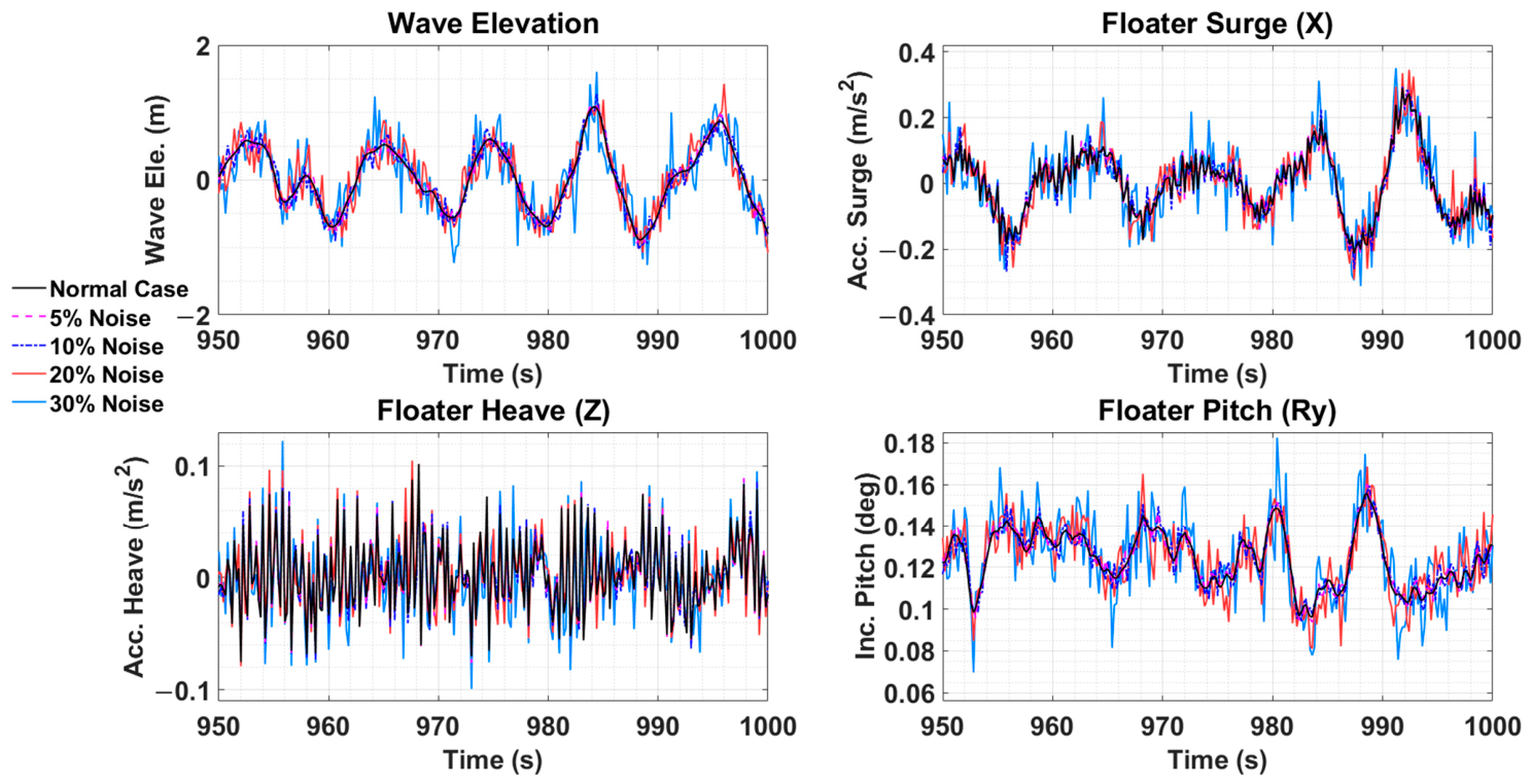
To reflect this consideration, the present study generated noisy datasets by adding Gaussian noise to the original input data in order to evaluate the sensitivity of the models against uncertainty. Especially, zero-mean Gaussian noise was independently added to each of the 16 input features, and the standard deviation of the added noise was set to a fixed percentage of the standard deviation of the corresponding noise-free input signal, where the standard deviation of each feature was computed separately for the training, validation, and test datasets. In the noise scenarios, a total of four cases were defined, corresponding to noise levels of 5%, 10%, 20%, and 30%. Here, a noise level of, for example, 5% indicates that the standard deviation of the added Gaussian noise equals 5% of the standard deviation of the corresponding noise-free signal. Specifically, Gaussian noise with uncertainty levels of 5%, 10%, 20%, and 30% was independently added to the original training, validation, and test input datasets. At this stage, noise injection was applied to the raw data prior to normalization.
Figure 10 presents a partial time-series comparison of the original input data for Training Case 07 and the corresponding data after the application of Gaussian noise. As observed in the figure, the addition of noise introduces noticeable high-frequency components compared to the original signal. Furthermore, it can be confirmed that the magnitude of these high-frequency components increases as the level of noise becomes larger.
The performance evaluation of the LSTM, GRU, and EN-ATT models was further conducted using the input datasets augmented with Gaussian noise. Accordingly, the performance of the three algorithms was comparatively analyzed under two distinct conditions: a nominal case without noise in the input data and noisy cases in which Gaussian noise was added to the input data. As described previously, the noisy cases were categorized into four levels of uncertainty: 5%, 10%, 20%, and 30%. Table 5 summarizes the classification of these cases.

4. Results

4.1. Learning Process by Epoch

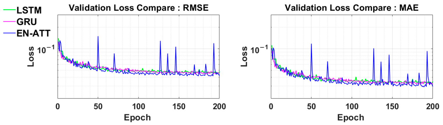
Training was conducted on the algorithms using the previously described parameters, and Figure 11 depicts the variation in the validation RMSE (used as the loss function) and MAE (as an auxiliary metric) across epochs for each algorithm in the normal case. In the graph, although EN-ATT occasionally showed spike peaks during training, its overall RMSE and MAE values remained lower than those of the RNNs throughout the training process, implying its potential for better predictive performance.
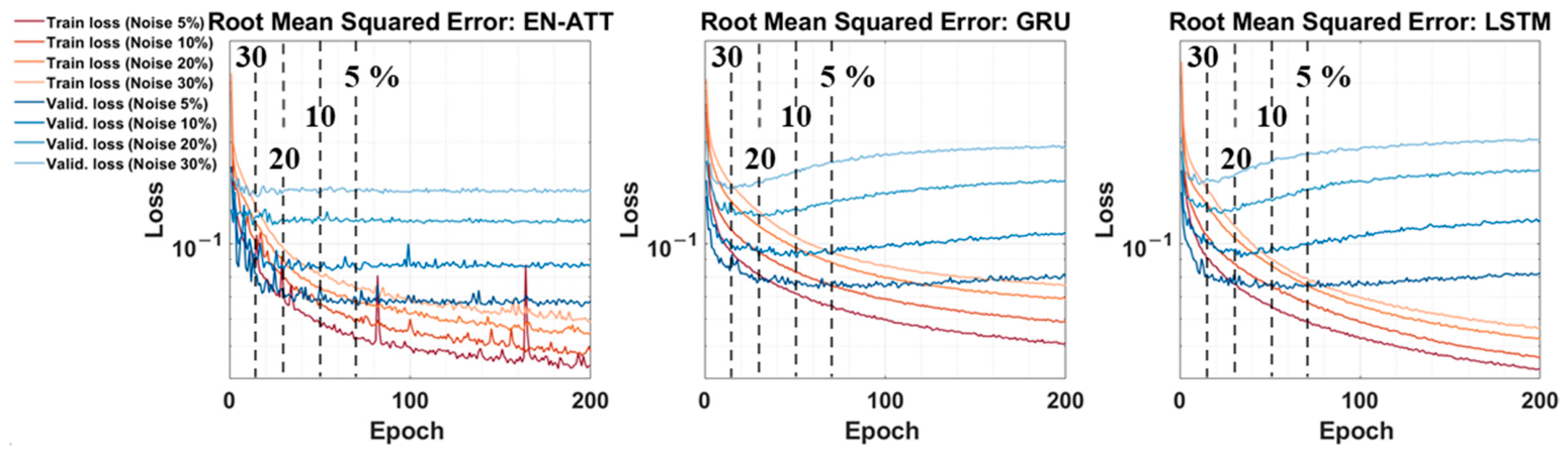
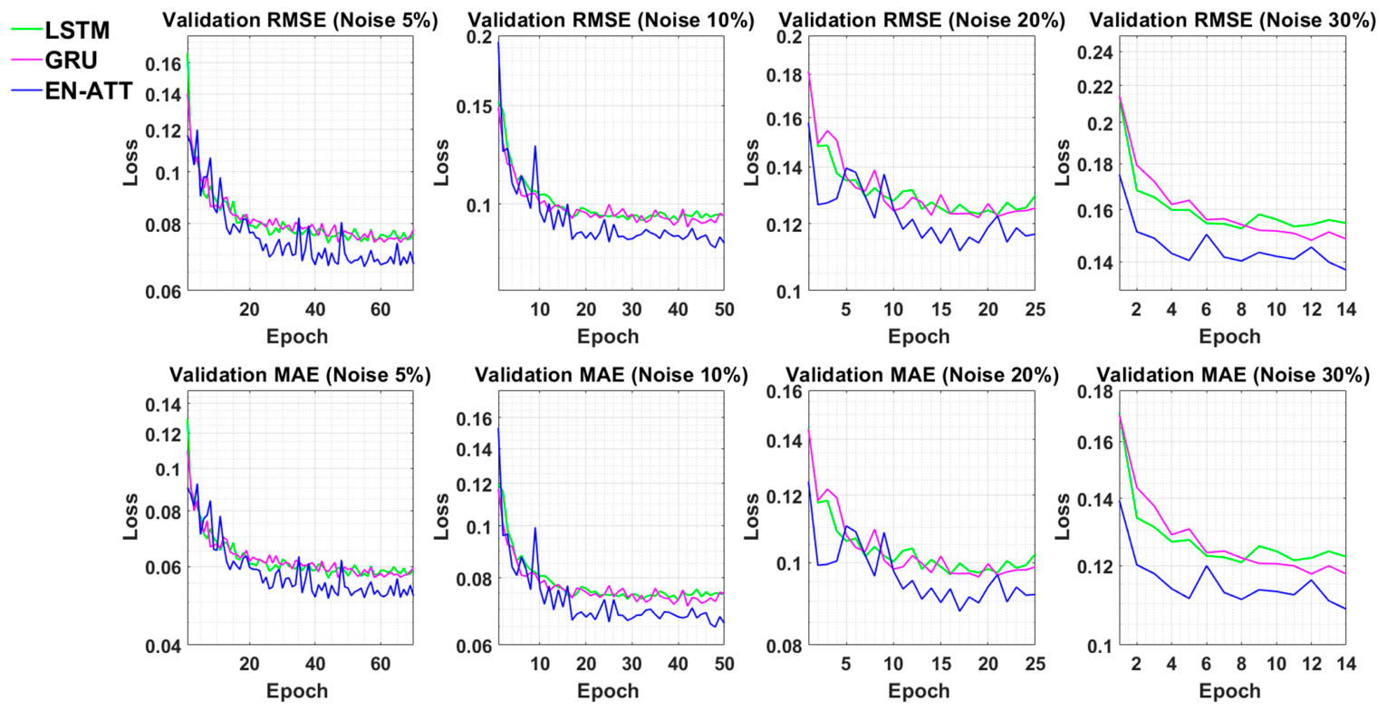
Figure 12 illustrates the training process under the noisy cases. Interestingly, when noise was introduced, overfitting was observed in the GRU and LSTM. In other words, as the number of epochs increased, the training loss continued to decrease, whereas the validation loss began to increase after a certain number of epochs. Moreover, this overfitting behavior became more pronounced as the noise level increased. In contrast, the EN-ATT model did not exhibit noticeable overfitting in the presence of noise, and both the training and validation losses tended to converge to relatively stable values.
Overfitting is generally associated with models that contain a large number of trainable parameters. However, as shown in Table 4, EN-ATT contains a larger number of trainable parameters than the RNNs considered in this study. Despite this, EN-ATT exhibited a more stable learning process under noisy conditions. These observations suggest that the improved performance may not be solely attributed to model size, but may also be related to the structural characteristics of the attention-based architecture.
To mitigate the aforementioned overfitting, the number of training epochs was adjusted according to each noise level. Similarly to the approach used in previous studies [11,12], the optimal epoch was selected as the epoch at which the validation loss appeared to be minimized, and retraining was subsequently performed. As indicated by the black dashed lines in Figure 12, retraining was conducted with 70, 50, 25, and 14 epochs for the 5%, 10%, 20%, and 30% noise levels, respectively.
Figure 13 presents the validation loss and MAE obtained after the retraining process. As shown in the figure, the overall validation loss values for all networks escalate correspondingly as the noise level increases. This trend indicates that the prediction performance deteriorates with the addition of noise. Notably, across all noise levels, EN-ATT tended to exhibit lower loss values than the conventional RNNs. Based on these observations, it is speculative that EN-ATT will also demonstrate comparable or better performance in the test cases.

4.2. Performance Comparison Under Nominal Conditions (Without Noise)

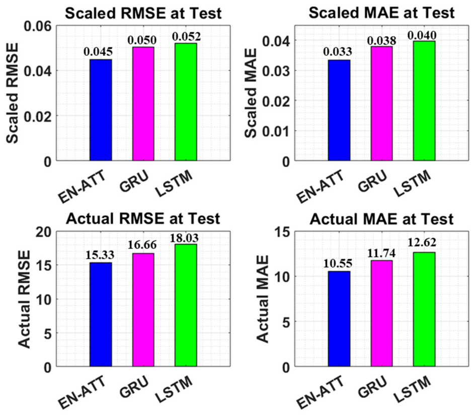
This section comparatively analyzes the performance of the three algorithms under nominal conditions. First, Figure 14 presents bar graphs showing the RMSE and MAE values of the three algorithms on the test dataset. The bar graph shows both the RMSE and MAE values calculated on data scaled with the standard-scaler, and the corresponding actual values obtained through inverse transformation of the scaled data. Test results revealed that the self-attention-based neural network EN-ATT achieved better performance, with lower RMSE and MAE values compared to the LSTM and GRU.
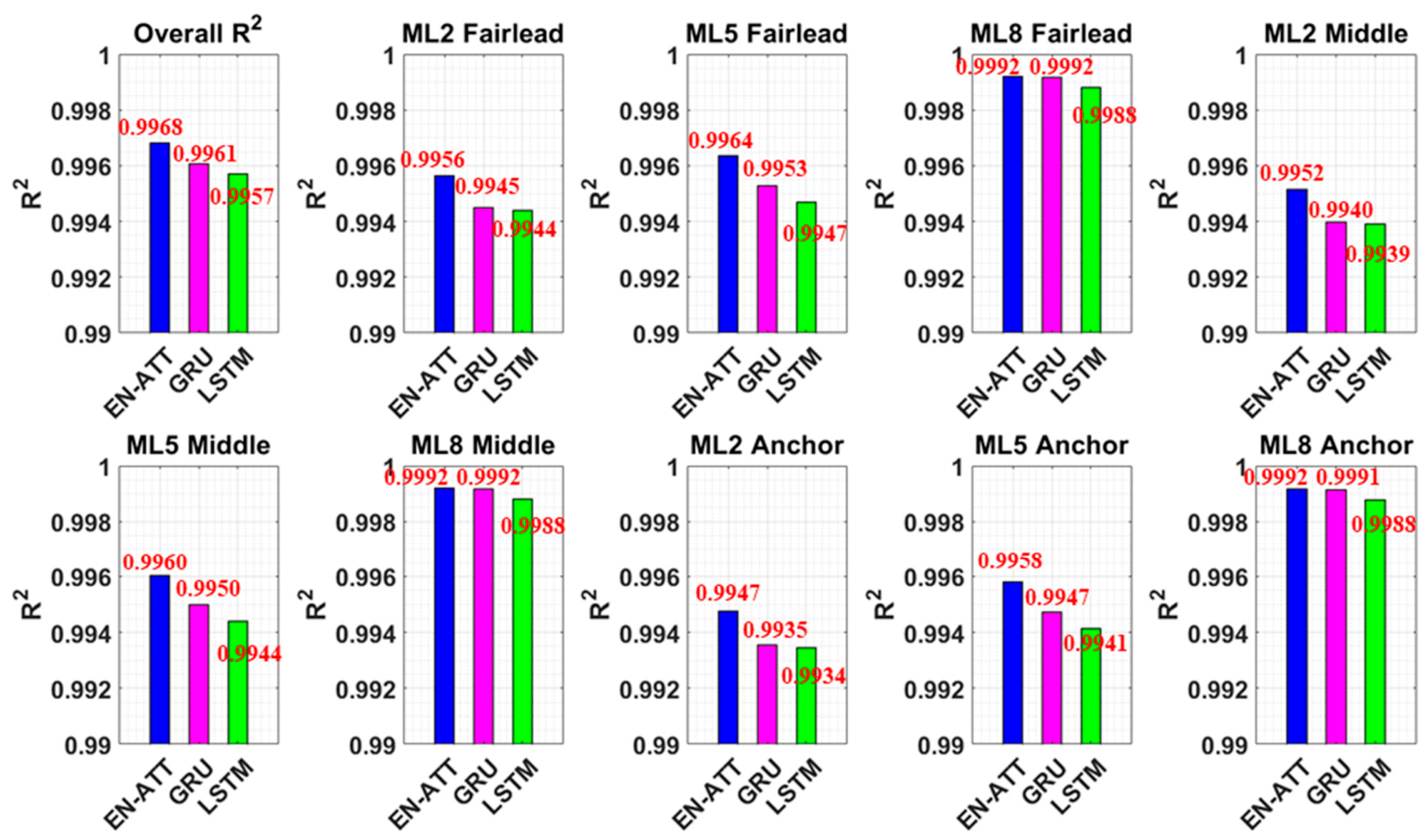
To conduct a more detailed analysis, the coefficient of determination ( R 2 ) was also compared. Figure 15 presents bar charts comparing the overall R 2 values as well as the R 2 values at each mooring tendon point. Consistent with previous results, the EN-ATT algorithm showed the highest overall R 2 value, followed by GRU and then LSTM.
For tendons #2 and #5, the R 2 decreased slightly from the fairlead to the middle and anchor targets. Because all target locations were predicted from the same input set, this comparison indicates only a small target-location difference and does not isolate sensor depth or sensor-to-target distance as its cause. The differences were marginal, and tendon #8 showed no consistent depth-dependent trend.
Next, scatter plots and residual distributions were examined. The residual ( e k ( n ) ) is defined as follows:
e k ( n ) = y k ( n ) y ^ k ( n )
where y k ( n ) denotes the actual value and y ^ k ( n ) denotes the predicted value. Here, k represents the k -th target feature, and n denotes the n -th temporal sample.
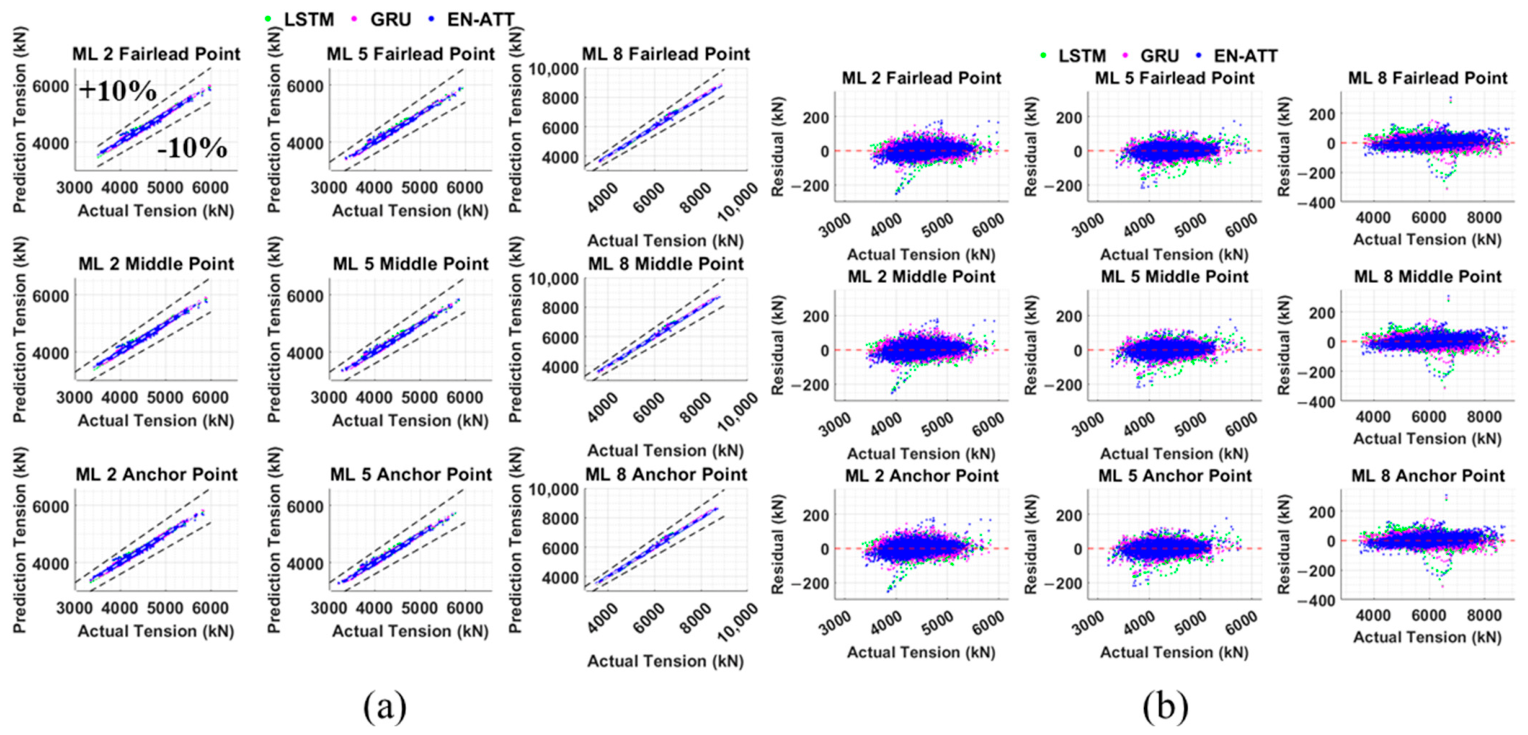
Figure 16 presents the scatter plots and corresponding residual distributions. In the scatter plots, data points from all three algorithms were tightly clustered around the target reference line, demonstrating the high fidelity of the trained models. Additionally, it was confirmed that the prediction error at all mooring tendon points remained within ±10%, demonstrating a high level of accuracy in the predictions. Notably, tendon #8 showed a tighter clustering around the dashed line compared to tendons #2 and #5, further confirming its superior predictive accuracy.
Across all networks, the residual distributions at the fairlead, middle, and anchor sections showed no noticeable differences. Moreover, the EN-ATT model exhibited a smaller spread of residuals within the main residual clusters than RNNs, indicating more tightly concentrated prediction errors.
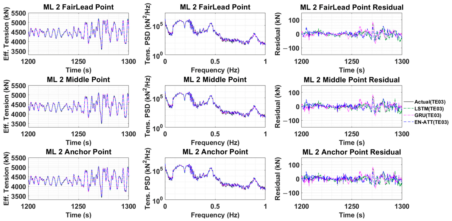
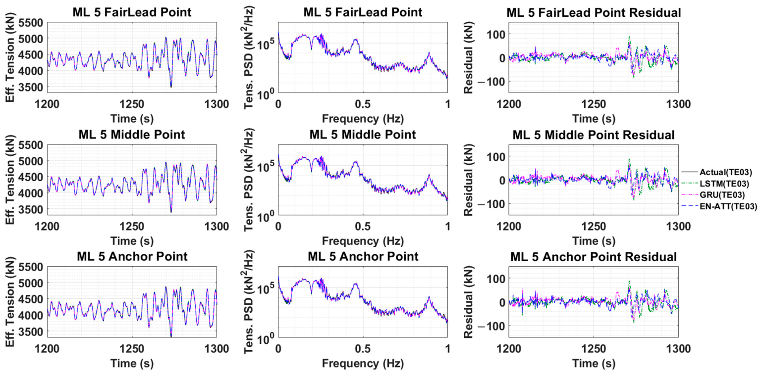
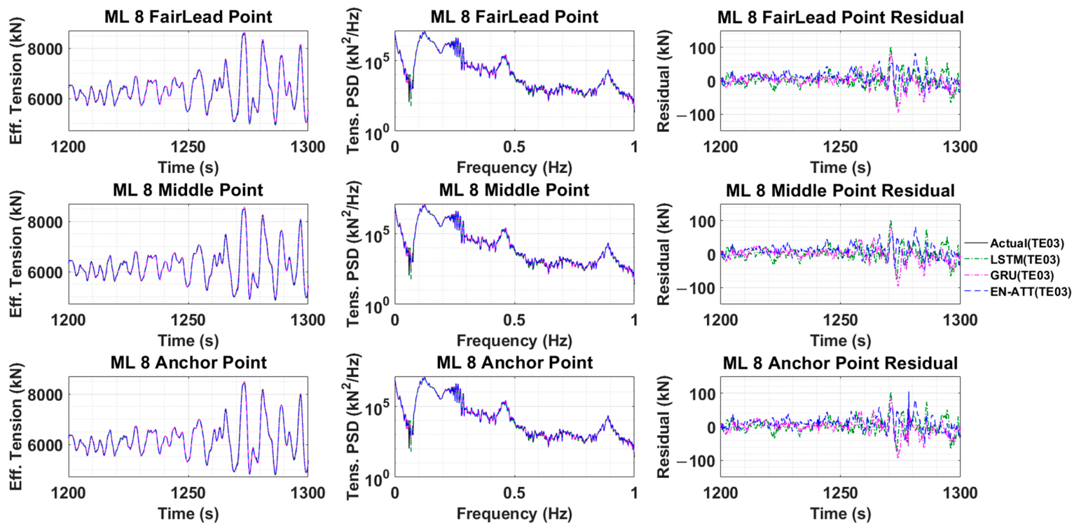
Next, the time-series responses of the effective tension and residuals, along with the PSD in the frequency domain, were analyzed. Figure 17, Figure 18 and Figure 19 illustrate the effective tension time series (1200~1300 s), residual distributions (1200~1300 s), and PSD (0~1800 s) for mooring tendons #2, #5, and #8 in Test Case 03, respectively.
The time series and PSD plots demonstrated that the predicted results exhibited high fidelity to the actual values. Moreover, the PSD results indicate that the tendon tension response is predominantly governed by the major frequency components, including the wave-frequency response around 0.2 Hz, the pitch natural-frequency response, and the blade natural-frequency response near 0.45 Hz (mode shapes in Supplementary Materials S5), all of which were well captured by the models. Additionally, due to the characteristics of the TLP mooring system, the mooring tensions at the fairlead, middle, and anchor points differed only by slight downward offsets as water depth increased. This demonstrated that the mooring tendon tensions below the surface can be adequately predicted using only near-surface sensor data.
Residual variability differed slightly among the fairlead, middle, and anchor targets. However, the differences were small, and tendon #8 showed no consistent depth-dependent pattern. The present results therefore do not establish a general relationship between prediction accuracy and target depth.

4.3. Performance Comparison Under Noisy Conditions

This section presents a comparison of the performance of the three algorithms evaluated under noisy conditions.
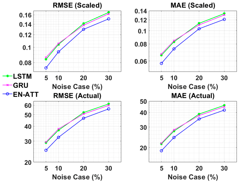
Figure 20 illustrates the RMSE and MAE obtained during the testing phase under the noisy conditions. As shown in the figure, the overall performance of all three algorithms deteriorated as the noise level increased. Nevertheless, EN-ATT yielded lower error values than the other models across all noise levels.
An interesting observation is that, for EN-ATT, the increase in error from 10% to 20% noise exhibited a steeper slope than that from 20% to 30%. This suggests that beyond a certain noise threshold, the rate of performance degradation may not increase proportionally and could become less pronounced. Furthermore, when comparing the LSTM and GRU, the difference in their test loss values was generally marginal.
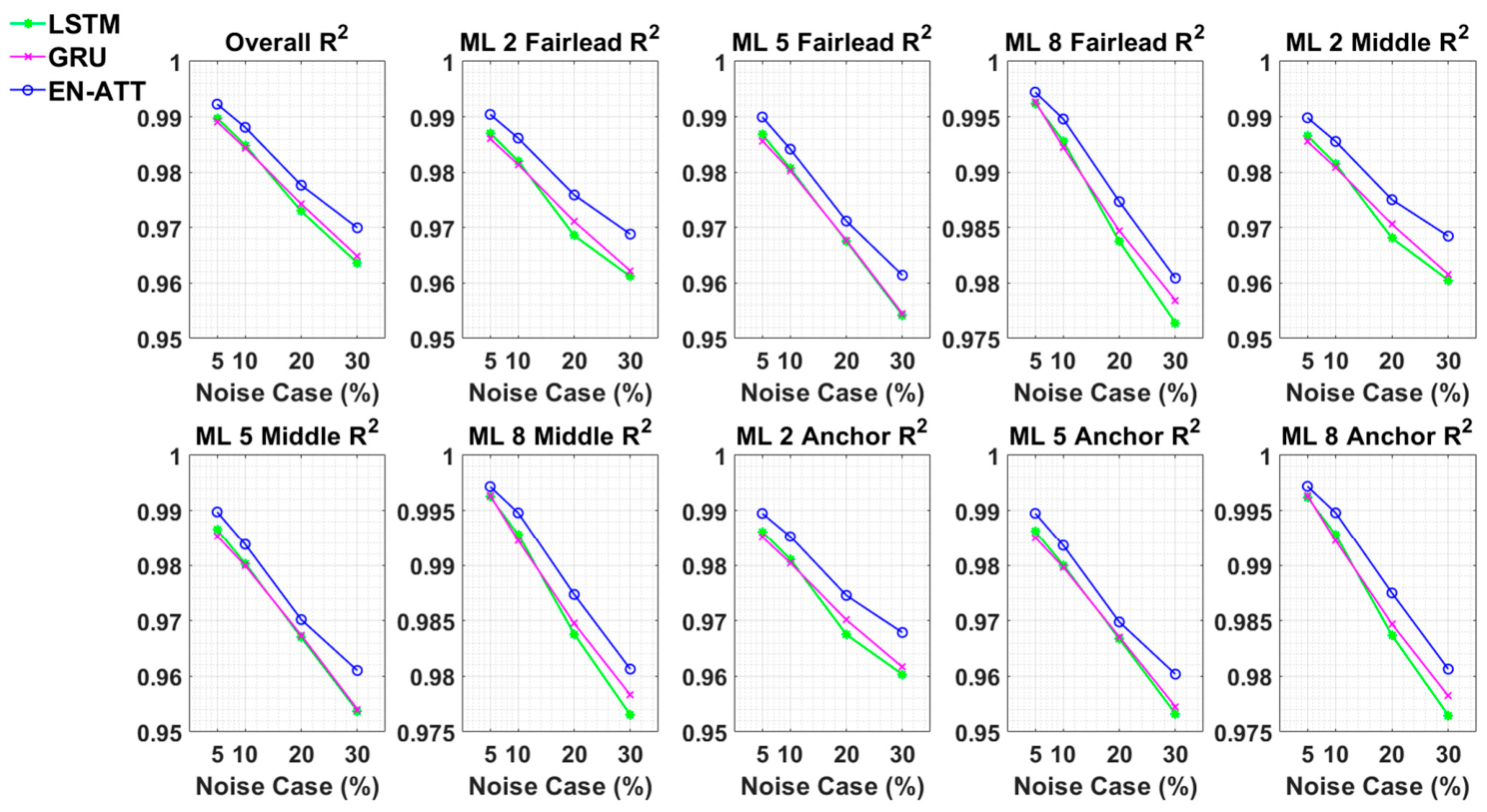
Subsequently, the coefficient of determination ( R 2 ) was evaluated. Figure 21 presents the R 2 values obtained under the noisy conditions. From an overall perspective, EN-ATT consistently achieved higher R 2 values than the conventional RNNs across all noise levels and prediction points.
A notable observation is that, for EN-ATT, the reduction in R 2 from 10% to 20% noise was greater than that from 20% to 30% noise at all prediction points of mooring tendons #2 and #5. This indicates that, for tendons #2 and #5, the rate of performance degradation became less pronounced as the noise level increased beyond 20%. In contrast, for mooring tendon #8, which directly faces wave loading, the magnitude of R 2 reduction between these two intervals appears to be similar.
In the case of GRU, the decreasing trend in Overall R 2 as well as at all prediction points remained relatively consistent as the noise level increased, compared to the other two algorithms. Furthermore, even at the highest noise level of 30%, all algorithms achieved an Overall R 2 exceeding 0.96.
Finally, Table 6 summarizes the R 2 values of EN-ATT. Similarly to the nominal (noise-free) case, for tendons #2 and #5, the R 2 values exhibited a slight decreasing tendency from the fairlead to the middle and anchor positions. For tendon #8, which is directly subjected to wave loading, no noticeable difference among prediction points is observed at the 5% and 10% noise levels. Under more severe noise conditions, slightly higher R 2 values were occasionally observed at greater water depths; however, these differences remained marginal.
Subsequently, the residual distributions were analyzed. Based on the results of Section 4.2 (nominal case) and the R 2 values obtained for the noisy cases, the tension predictions at the fairlead, middle, and anchor positions exhibited similar trends, with only minor tension offsets. Therefore, for clarity and conciseness, only the residual distributions at the anchor position—presumed to show relatively lower performance among the three locations—are presented.
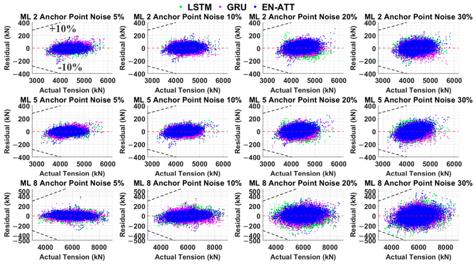
Figure 22 illustrates the residual distributions of the anchor tension for mooring tendons #2, #5, and #8 according to the noise level. As observed in the figure, the variation of the residuals increased progressively as the noise level became higher. This trend further suggests that predictive performance deteriorated with increasing noise levels. Notably, for tendon #8, which directly faces wave loading, the increase in residual variation with higher noise levels was more pronounced compared to the other tendons.
Interestingly, across all cases—including the 30% noise level—all algorithms produced predictions within ±10% of the actual values. Finally, when comparing the three algorithms, EN-ATT exhibited the primary residual cluster more closely centered around zero than the other networks, indicating superior predictive accuracy.
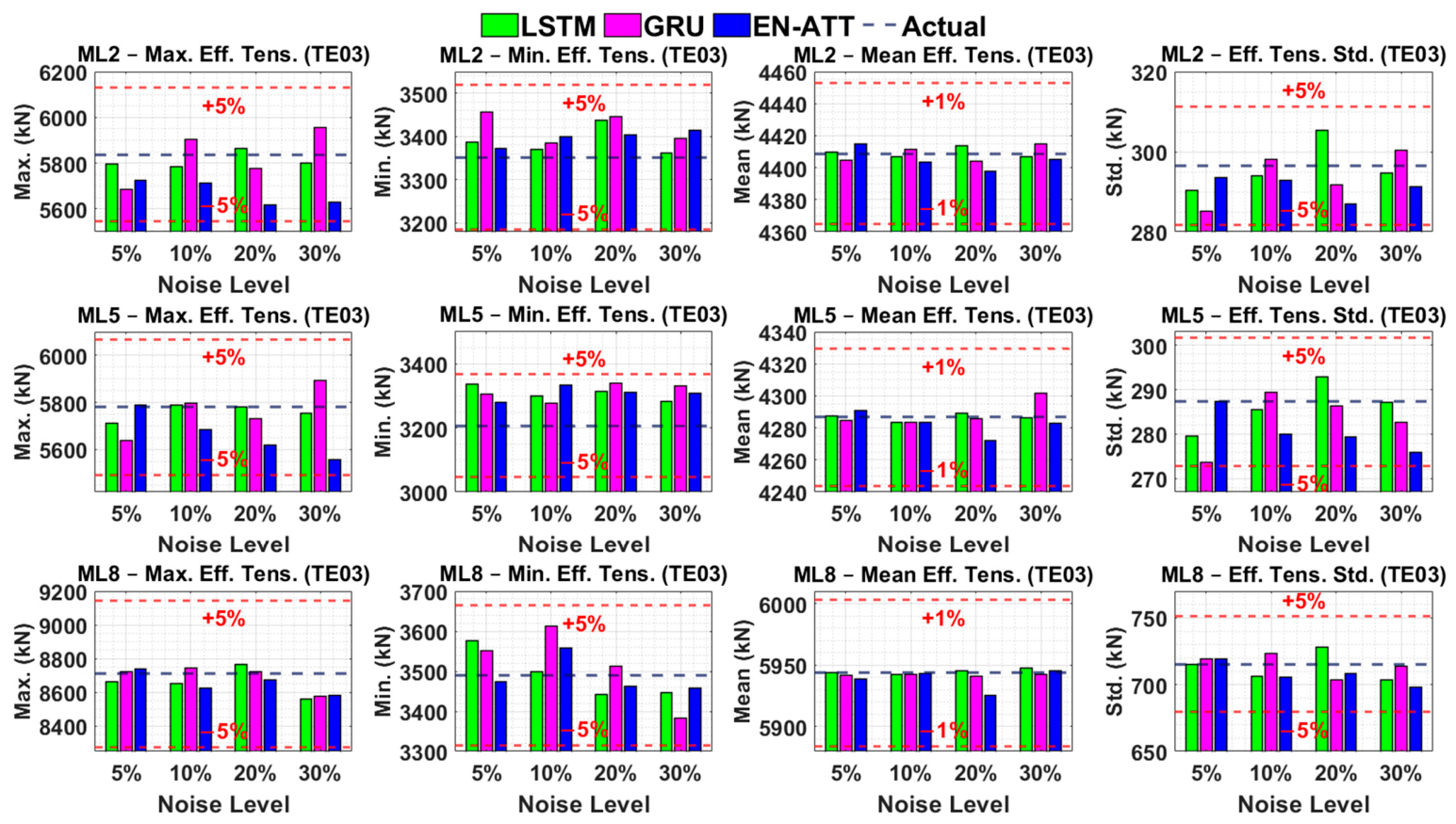
For a more detailed comparison, additional statistical metrics were examined. Figure 23 presents bar charts of the maximum, minimum, mean, and standard deviation values at the anchor positions of mooring tendons #2, #5, and #8 for Test Case 03. From the figure, it was observed that the maximum, minimum, and standard deviation values predicted by all algorithms fell within 5% of the corresponding actual values, even at the highest noise level of 30%. Furthermore, the mean values predicted by all algorithms remained within 1% of the actual values.
An interesting observation arises when comparing the maximum and minimum values. Although EN-ATT demonstrated the highest performance in terms of RMSE and R 2 in the previous evaluation metrics, its predictions of extreme values (maximum and minimum) did not consistently outperform those of the other algorithms. This suggests that superior performance in RMSE and R 2 does not necessarily guarantee more accurate prediction of extreme values.
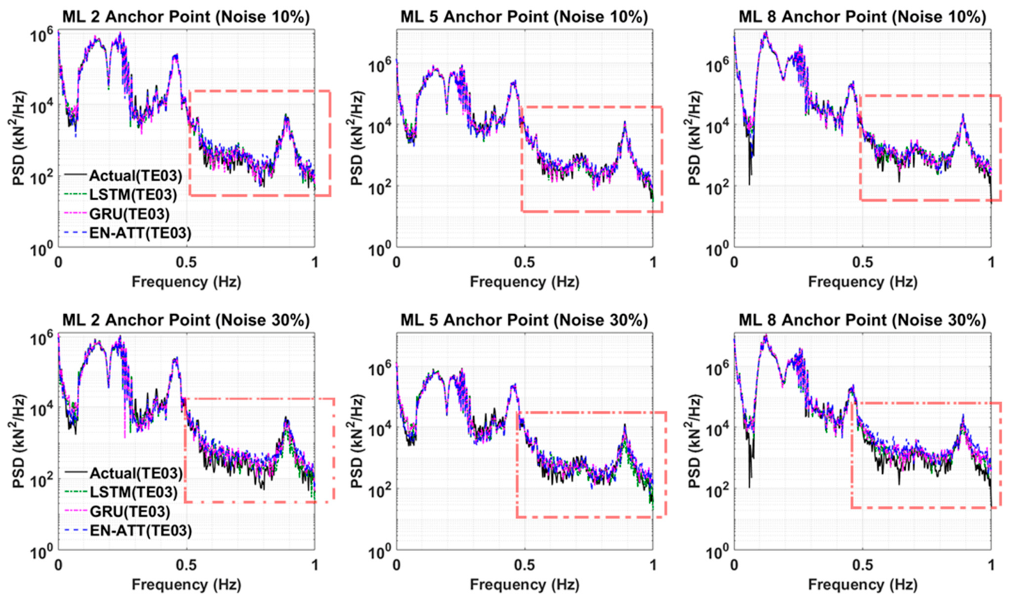
Subsequently, the time-series responses and corresponding PSD results were examined. For the time-series analysis, the case with the largest residual variation—namely, the 30% noise level—was selected. In contrast, the PSD results were analyzed for the 10% and 30% noise levels.
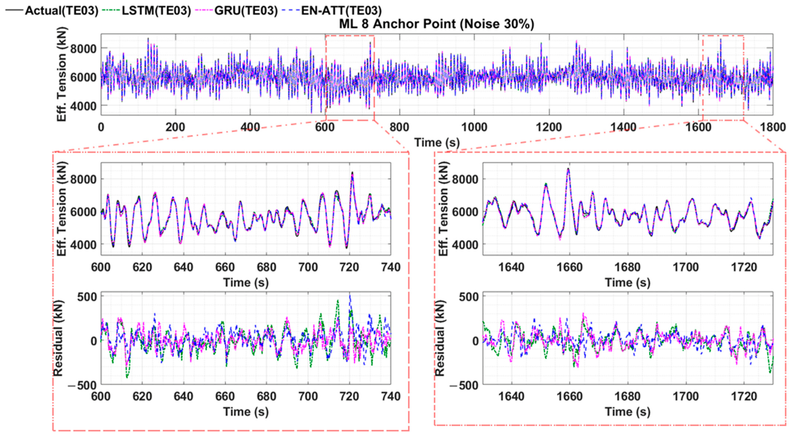
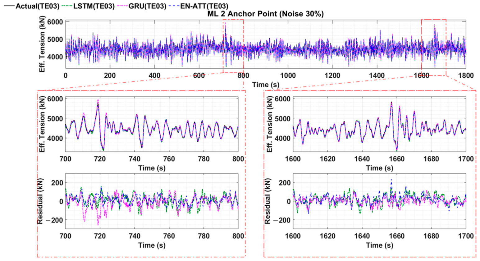
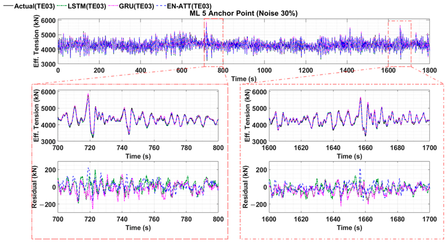
Figure 24, Figure 25 and Figure 26 present the effective tension time-series responses at the anchor points of tendons #2, #5, and #8, respectively, under the 30% noise condition. As shown in the figures, a good agreement was observed in the time domain. Upon examining the residual responses, the residuals for tendons #2 and #5 were maintained within approximately ±200 kN. In contrast, for tendon #8, which directly faces wave loading, the residuals remained within approximately ±500 kN.
It was also observed that the residual time-series patterns varied slightly among the algorithms. In particular, the absolute residual values increased during sudden tension variations, indicating that predictive performance may deteriorate in regions characterized by rapid tension changes. For EN-ATT, positive residuals were observed during sudden tension increases, implying that the predicted tension was lower than the actual value in these regions.
This further suggests that, despite strong overall performance metrics, the prediction of extreme or rapidly varying responses may still be limited. Similar tendencies were also observed for LSTM and GRU, which exhibit larger residuals during abrupt tension transitions. Nevertheless, even under this extreme noise level, the overall time-series agreement remained reasonably good.
Figure 27 illustrates the PSD of the effective tension at the anchor points of tendons #2, #5, and #8. From the PSD results, it was confirmed that the primary peaks—namely, the wave-frequency response around 0.2 Hz, the pitch natural frequency response, and the blade natural frequency response near 0.45 Hz—were well predicted, similar to the nominal case. An interesting observation is that, as the noise level increases, prediction accuracy at higher-frequency regions (red dashed box in Figure 27) tends to deteriorate due to high-frequency disturbances. However, a dominant peak around 0.9 Hz was consistently well captured across all noise levels.

5. Discussion

5.1. Overall Discussions

This section discusses the results presented in Section 4. First, under the nominal condition, EN-ATT demonstrates higher predictive performance than the RNNs in terms of RMSE, MAE, and R 2 . In addition, across all neural networks, almost no noticeable performance differences are observed among the fairlead, middle, and anchor positions. This behavior is likely associated with the strong pretension characteristic of the TLP system. These results indicate that unmeasured underwater tendon tension can be reasonably estimated using sensor data that are readily obtainable near or above the water surface.
In the noisy cases, the predictive performance of all neural networks decreases as the noise level increases, while EN-ATT consistently showed lower RMSE and MAE, and higher R 2 , than the RNNs across all noise levels. However, in the prediction of extreme responses, such as sudden tension changes or maximum and minimum tension values, EN-ATT does not always guarantee superior performance compared to RNNs. Therefore, further analysis of the internal characteristics of the neural networks is conducted using the feature gradient analysis defined in Section 3.3 (Section 5.2), followed by a comprehensive evaluation presented in Section 5.3.

5.2. Neural Network Internal Characteristics and Physical Interpretation of System Dynamics Based on Feature Gradient Analysis

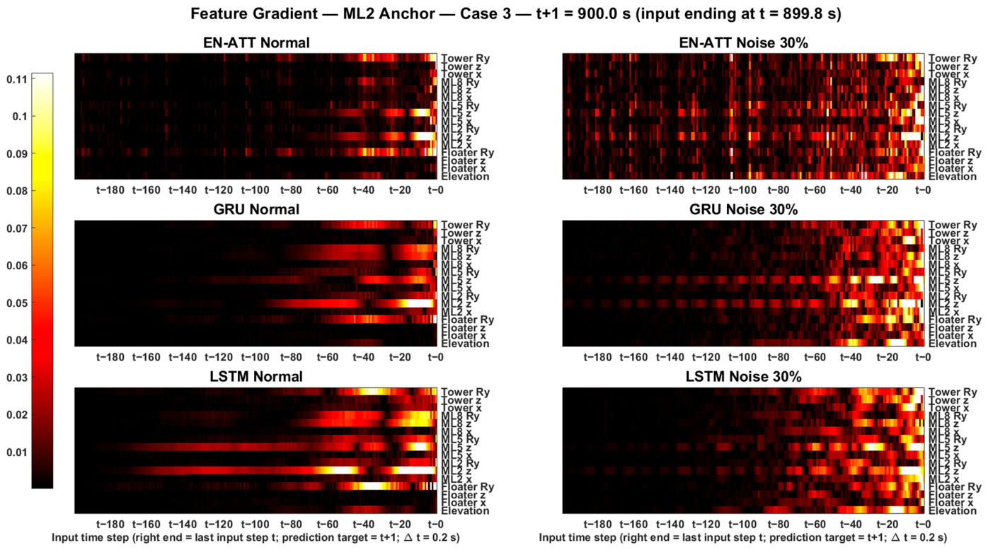
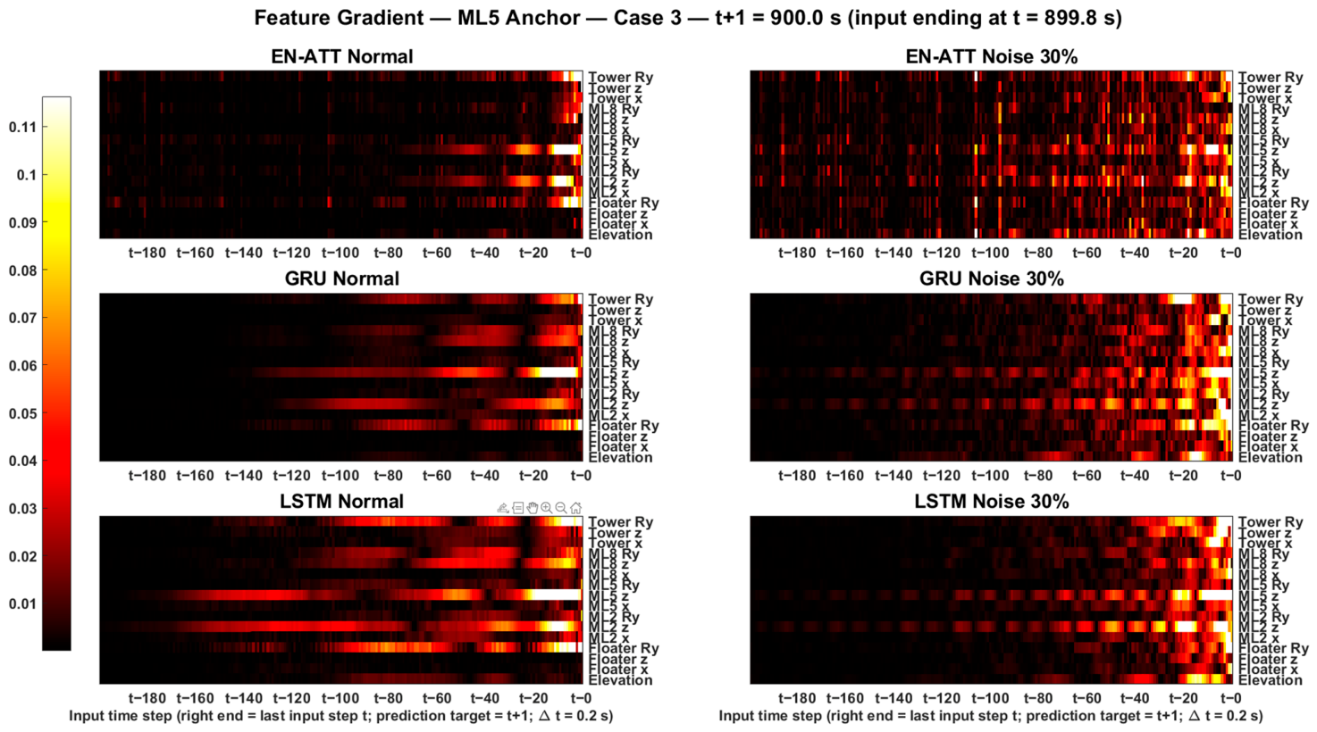
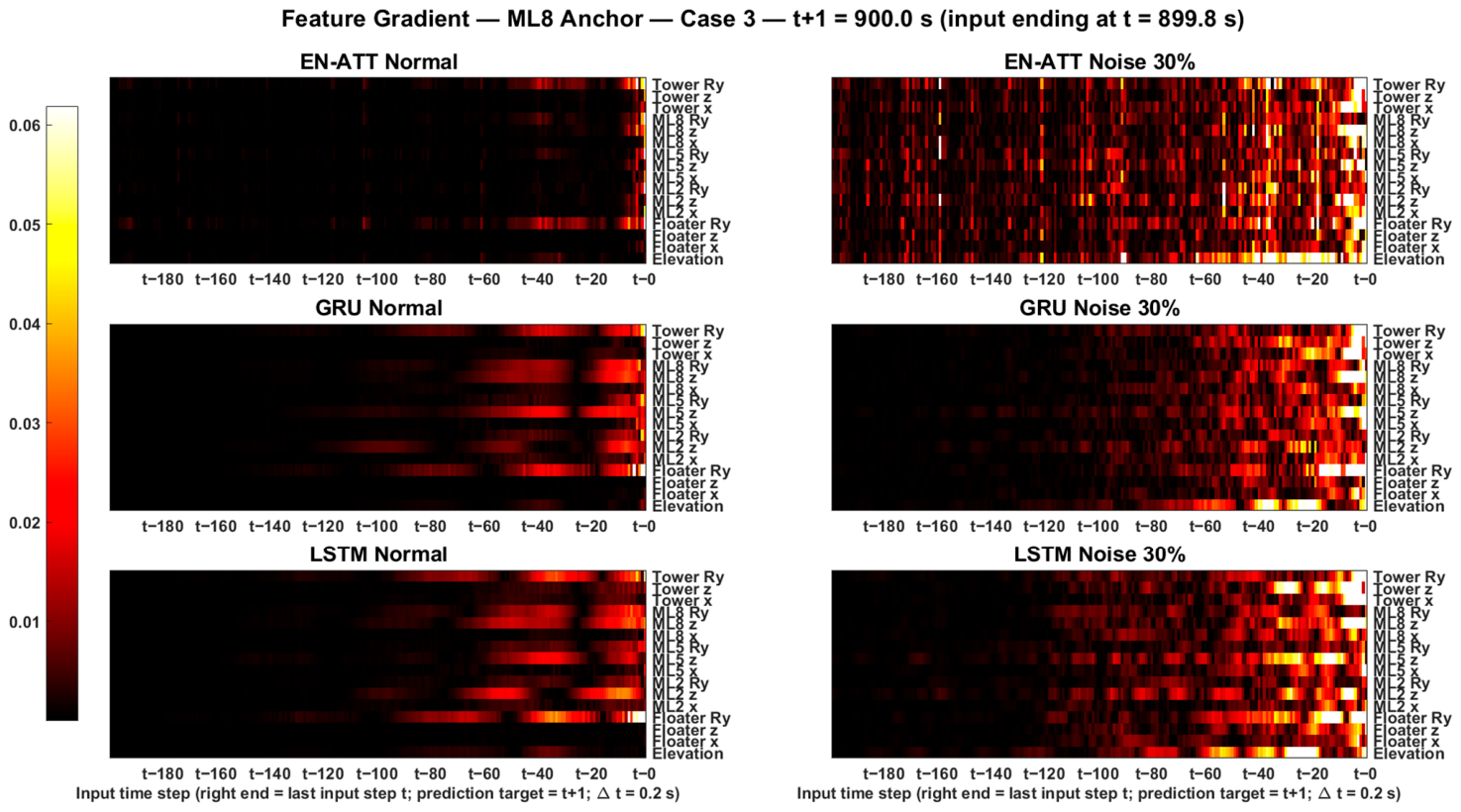
This section discusses the internal learning characteristics and physical interpretability of the neural networks based on the results presented above. To ensure a fair comparison in the feature gradient analysis, all models were retrained under identical hyperparameter settings. Figure 28, Figure 29 and Figure 30 present the feature gradients with respect to input timesteps at the points of tendons #2, #5, and #8 for the nominal and 30% noise cases, respectively (extracted at 900 s of the test case). The color scale is restricted to the 1st–99th percentile range to suppress extreme outliers and enhance interpretability. Additionally, videos illustrating the temporal evolution of the feature gradients over time are provided in Supplementary Materials S3.

5.2.1. Physical Interpretability in Nominal Conditions

As shown in Figure 28, Figure 29 and Figure 30 under the nominal condition, both the RNN-based models and EN-ATT exhibit prominent gradients in the most recent timesteps, indicating that tendon tension is primarily predicted based on recent response patterns.
A more detailed analysis shows that, in Figure 28 and Figure 29, tendon tension prediction mainly depends on the floater pitch response, the heave responses of tendons #2 and #5, and the tower pitch response. This suggests that the networks learn response patterns consistent with the dynamics of the TLP system, where mooring tendons restrain vertical motion while experiencing increased tension.
In the case of EN-ATT, the heave-direction gradients of tendons #2 and #5 are particularly prominent within the last ~10 timesteps before the prediction point, suggesting that the model reflects patterns associated with the system’s heave natural frequency (0.6658 Hz ≈ 1.502 s ≈ 7 timesteps × 0.2 s).
Moreover, noticeable gradients appear around 20 timesteps, likely related to the pitch natural frequency (0.2558 Hz ≈ 3.909 s ≈ 20 timesteps × 0.2 s). For the pitch responses, prominent gradients occur both immediately before the prediction point and around 40 timesteps, corresponding to the dominant wave period of Test Case 03 (8.5 s ≈ 42 timesteps × 0.2 s), indicating that the network captures the wave-induced response pattern.
In Figure 30, for tendon #8 facing wave loading, the nominal case indicates that the networks mainly capture the floater and tower pitch responses.

5.2.2. Noise Sensitivity and Shift in Input-Feature Sensitivity

When noise is introduced, all networks incorporate additional input features. Furthermore, in Figure 28 and Figure 29, the heave responses of tendons #2 and #5 form distinct gradient bands at ~7-timestep intervals across all networks, corresponding to the heave natural frequency. This is consistent with the networks capturing the system’s underlying physical response patterns even under severe noise.
Notably, EN-ATT exhibits pronounced gradient magnitudes at distant timesteps (~160–200), which lie in the vicinity of the system’s surge natural period (0.03536 Hz ≈ 28.3 s ≈ 141 timesteps × 0.2 s) and the associated low-frequency slow-drift response. Compared to the RNN-based models, EN-ATT showed greater gradient sensitivity to distant timesteps under noisy conditions, suggesting that its predictions may draw on longer-range temporal information.
Overall, as input noise increases, the networks rely more on wave elevation patterns for tension prediction, whereas motion responses dominate in the nominal case. This tendency is most pronounced for tendon #8 facing wave loading, suggesting that incorporating wave elevation can improve predictive performance under noisy conditions.
Although caution must be exercised when simply associating feature gradients with human physical intuition or concluding that the network has directly learned physical laws [23], sound engineering judgment combined with domain knowledge [14], such as the natural frequencies of the system, can improve the physical interpretation of the network in relation to the underlying system dynamics.

5.3. Comprehensive Evaluation

Consequently, EN-ATT generally showed better performance than conventional RNNs in RMSE, MAE, and R 2 under both nominal and noisy conditions. However, it does not always provide better predictions for extreme values or abrupt tension surges and requires more trainable parameters than RNNs.
The limited advantage of EN-ATT for extreme values and abrupt tension changes can be attributed to three factors. First, all models were trained with RMSE, which is dominated by the abundant samples near the mean of the tension distribution; a model therefore minimizes the loss most efficiently by fitting the bulk of the distribution, and rare maxima and minima tend to be under-predicted regardless of architecture. Second, the self-attention output is a softmax-weighted average of the value vectors over the input window (Equation (13)), and this averaging tends to smooth abrupt transitions, which is consistent with the positive residuals of EN-ATT observed during sudden tension increases (Figure 24, Figure 25 and Figure 26). Third, the training cases represent normal operating sea states, so extreme tension excursions constitute only a small fraction of the training samples, limiting how well any of the three networks can learn the tails of the distribution.
In contrast, feature gradient analysis shows that EN-ATT exhibits larger input sensitivities at long input lags than the RNNs, while remaining highly sensitive to recent timesteps.
These findings indicate that EN-ATT has greater representational flexibility and learning potential than RNNs, with sensitivity spanning both short and long input lags. This suggests that self-attention-based networks can provide a flexible framework consistent with known dynamic response features, warranting further investigation.
From a practical monitoring perspective, point-by-point agreement of the entire tension time series is not the only relevant measure of fidelity. For tendon condition monitoring, the reconstructed signal should also preserve the overall load level, variability, extreme tension excursions, and fatigue-relevant cyclic content. No universally accepted accuracy threshold is currently available for machine-learning-based virtual sensing of FOWT tendon tension; therefore, the present study does not interpret a specific error level as a certification criterion. Instead, the ±5% range used in the statistical and DEL comparisons were employed as an indicative engineering reference for evaluating the practical fidelity of the reconstructed signals.
Under this reference, all three models reproduced the maximum, minimum, and standard deviation of the tendon tension within approximately 5% of the reference values, while the mean tension remained within approximately 1%, even under the 30% input-noise condition. In addition, the overall coefficient of determination remained above 0.96 for all models. The indicative DEL comparison further showed that the fatigue-relevant content was generally reproduced within ±5%, although several cases for tendon #5 slightly exceeded this range. These results suggest that all three architectures provide a comparable level of fidelity for reconstructing the principal characteristics of the tendon response under the conditions considered in this study. Although EN-ATT provides better overall RMSE, MAE, and R 2 values, its practical advantage over the recurrent models is less pronounced when extreme-value and fatigue-relevant measures are considered. Therefore, the results should be interpreted as demonstrating the feasibility of the virtual sensing framework rather than establishing that one architecture is universally superior for practical monitoring.

6. Limitations and Future Work

Nevertheless, several limitations remain in the present study. First, because the dataset was generated from numerical simulations, there may be discrepancies from real offshore operating conditions. In addition, an indicative DEL comparison for a single sea-state realization is provided in Appendix A; its limitations are discussed therein.
Second, the wind and current conditions were fixed across all cases (near-rated wind speed of 10 m/s with a single turbulence realization) in order to isolate the effect of the wave condition, and only unidirectional environmental loading was assumed. In reality, the mean wind speed varies jointly with the sea state; future work will therefore sample correlated wind–wave conditions from a joint probabilistic model of wind speed, significant wave height, and peak period, including above-rated and parked conditions.
Third, the analysis was restricted to the operational (power-producing) state of the FOWT. In addition, turbine operational parameters, such as rotor speed, blade pitch angle, generator torque, and power output, were not included as input features in the present study. The mean tendon tension may, in principle, be partly inferred from the initial pretension and turbine operating condition, potentially reducing the need for a machine learning model for estimating the mean level alone. Accordingly, the practical role of the present virtual sensing approach is primarily associated with reconstructing the dynamic tension fluctuations at submerged and unmeasured tendon locations rather than simply estimating the mean tension level. Readily measurable turbine operational parameters may also provide additional information regarding the turbine operating state and aerodynamic loading, and their contribution to tendon tension estimation should be systematically evaluated in future work.
In practical applications, predicting mooring tension under extreme environmental conditions is equally important, particularly when accurate estimation of extreme and maximum tension values is required. In this regard, although the EN-ATT did not consistently outperform the RNNs in every aspect, its greater sensitivity to long input lags suggests that self-attention architectures merit further investigation for this task.
Fourth, only the in-plane responses were used as inputs. Sway and roll are negligible under unidirectional loading. Yaw was excluded to reduce reliance on the most obvious shared wind-specific signal; however, this exclusion does not eliminate dependence on the common turbulence realization because the other inputs and targets also contain wind-induced components. The reported test performance therefore represents generalization across the selected wave conditions under a fixed wind realization, not to unseen turbulence realizations. Future work will assign independent turbulence seeds to each case and will include all six DOFs under multidirectional loading.
To address these limitations, future research will focus on developing self-attention-based neural networks capable of monitoring mooring tendon tension under multidirectional environmental loading conditions, extreme environmental scenarios, and turbine parked states. In particular, efforts will be directed toward improving predictive accuracy for extreme values and sudden tension variations by introducing extreme-aware training objectives, such as error-weighted or quantile losses, and by augmenting the training set with severe sea states. Additionally, research will be conducted on predictive performance when various sensor failure situations occur, not just sensor noise.

7. Conclusions

In this study, three deep learning architectures—a self-attention network (EN-ATT), LSTM, and GRU—were comparatively evaluated for estimating the mooring tension of a 15 MW TLP-type FOWT. The models were developed under the assumption that the FOWT operates in a power-producing condition.
The main conclusions derived from this study are summarized as follows.
  • In the nominal case, the self-attention-based network achieved lower loss function values and higher R 2 values than LSTM and GRU. Furthermore, due to the inherent characteristics of the TLP mooring system, the differences in mooring tension among the fairlead, middle, and anchor points exhibit only a slight downward deviation as the water depth increases. As a result, in the nominal case, all three neural networks were able to accurately predict the dynamic tension at submerged points using only sensors located above or near the free surface.
  • In the noisy cases, the self-attention-based network again outperformed the RNNs in terms of evaluation metrics. Moreover, the differences in R 2 values among the prediction points were found to be marginal.
  • When examining the maximum, minimum, mean, and standard deviation values under noisy conditions, EN-ATT did not consistently demonstrate superior predictive performance compared to the RNNs. This finding indicates that higher evaluation metric scores do not necessarily guarantee better predictive accuracy in all aspects, particularly for extreme values.
  • From the time-series and PSD analyses, all neural networks exhibited good overall agreement with the reference results. However, EN-ATT occasionally underestimated the tension during abrupt tension surges. RNNs also showed large residuals during sudden tension variations. In the PSD analysis, prediction performance in higher-frequency regions deteriorated as the noise level increased.
  • Feature gradient analysis suggested that the neural networks primarily learned response patterns associated with vertical motions of the TLP system and its tendon, such as heave and pitch. In addition, under highly noisy conditions, wave elevation patterns were also captured more prominently in the learning process. Consequently, EN-ATT exhibited feature gradient sensitivity extending to longer input lags than the RNNs, suggesting that it may utilize a wider temporal range of the input window.
Based on these findings, the EN-ATT model showed comparable or slightly better overall performance compared to RNNs. Although EN-ATT does not consistently achieve higher accuracy during abrupt tension variations, it showed greater sensitivity to longer input lags than the LSTM and GRU under the present experimental setting. From this perspective, further development of self-attention-based neural networks appears to be a worthwhile direction for future research.

Supplementary Materials

The following supporting information can be downloaded at: https://www.mdpi.com/article/10.3390/jmse14181745/s1.

Author Contributions

Conceptualization, S.M.K. and W.C.C.; methodology, S.M.K.; software, S.M.K.; validation, S.M.K., B.K. and W.C.C.; formal analysis, S.M.K.; investigation, S.M.K. and B.K.; resources, B.K. and W.C.C.; data curation, S.M.K. and B.K.; writing—original draft preparation, S.M.K.; writing—review and editing, B.K. and W.C.C.; visualization, S.M.K.; supervision, B.K. and W.C.C.; project administration, W.C.C.; funding acquisition, W.C.C. All authors have read and agreed to the published version of the manuscript.

Funding

This research was supported by Korea Institute of Marine Science & Technology Promotion (KIMST) funded by the Ministry of Oceans and Fisheries (RS-2025-02304428).

Data Availability Statement

The simulation datasets generated and analyzed during this study, as well as the source code of the neural network models developed in this study, are available from the author upon reasonable request. The detailed specifications and design data of the 15 MW TLP-type FOWT platform were provided by KRISO (Korea Research Institute of Ships and Ocean Engineering) and KIER (Korea Institute of Energy Research) and cannot be shared; publicly available information on the platform can be found in the referenced literature [28,29,30].

Acknowledgments

During the preparation of this work, the authors used ChatGPT (OpenAI; version GPT-5.6) and Claude (Anthropic; version Fable 5) to assist with translation and grammar/spelling checks. After using these tools, the authors reviewed and edited the content as needed and take full responsibility for the content of the published article.

Conflicts of Interest

The authors declare no conflicts of interest.

Appendix A. Indicative DEL Comparison for a Single Sea State

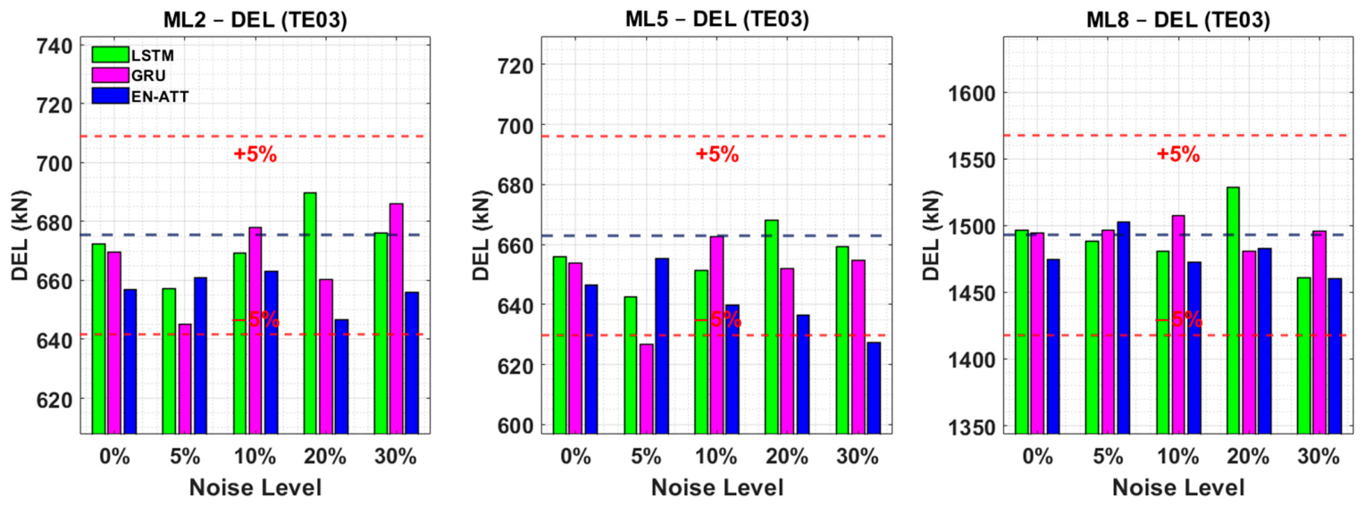
The fatigue-relevant content of the reconstructed signals was examined through the damage equivalent load (DEL), computed from the raw predicted and reference anchor-point tension series using the built-in rainflow function in MATLAB (version R2023b) [55], with an S–N slope of m = 4.0 for stranded rope [56] and a reference count of 1800 cycles, corresponding to an equivalent frequency of 1 Hz over the 1800 s record. DEL is reported in load units (kN).
Figure A1 compares the DELs obtained from the predicted and reference anchor-point tensions for tendons #2, #5, and #8 under the considered noise levels. For all three models, the predicted DELs remain close to the reference values and generally lie within the tolerance band indicated in the figure, although a few cases for tendon #5 slightly exceed it. The agreement is closest for the fatigue-critical tendon #8, which carries the largest tension.
The DEL is reported as a signal-level indicator only; its conversion into fatigue damage or life requires design-specific parameters not addressed here. As the results are based on a single sea-state realization, assessment across diverse sea states is left for future work.
Figure A1. Damage equivalent load (DEL, kN) of the anchor-point effective tension for tendons #2, #5, and #8 under input noise levels of 0–30% (Test Case 03). Dashed lines indicate the actual (reference) DEL and the ±5% band.
Jmse 14 01745 g0a1

Appendix B. Parameter-Matched Comparison

To examine whether the performance differences among the models originate from architectural characteristics rather than from differences in model capacity, a parameter-matched comparison was conducted. Two complementary variations were considered. First, the EN-ATT was reduced to a smaller configuration (“lower”, 68,617 parameters), comparable to the original GRU and well below the original LSTM, to test whether its accuracy persists at a reduced capacity. Second, the LSTM and GRU were enlarged (“matched”, ≈390,000 parameters) to approximately the size of the original EN-ATT, to test whether increasing their capacity closes the performance gap. All other settings (timestep = 200, batch size = 128, Adam optimizer, learning rate = 0.001, 200 epochs) were kept identical to the original models; only the numbers of layers, units, attention stacks, and attention heads were varied. The detailed configurations of the reduced and enlarged models are listed in Table A1.
Table A2 summarizes the trainable parameters and test performance of the original, reduced, and enlarged models. At this reduced capacity, the EN-ATT (“lower”, 68,617 parameters) attains an overall R2 of 0.9962 (actual RMSE 16.95), which remains comparable to the original LSTM (R2 0.9957, RMSE 18.03) and GRU (R2 0.9961, RMSE 16.66) despite its substantially smaller size. Conversely, enlarging the recurrent models to a comparable capacity does not close the gap to the full EN-ATT (R2 0.9968): the parameter-matched LSTM (387,401 parameters) remains essentially unchanged from its original configuration (R2 0.9958), and the parameter-matched GRU (396,489 parameters) exhibited divergent training (R2 = 0.7946), consistent with the divergence observed for the high-capacity GRU during the hyperparameter tuning (Supplementary Materials S1). These results suggest that, within the range examined, the predictive performance is associated more with the model architecture than with the number of trainable parameters.
Table A1. Configurations of the reduced (“lower”) and enlarged (“matched”) models.
ModelConfigurationTotal Number of Trainable Parameters
EN-ATT (lower)Up = 64, H = 8, FFN = 128, 2 stacks68,617
LSTM (matched)128–128–128–64 (units, 4 layers)387,401
GRU (matched)256–128–64 (units, 3 layers)396,489
Table A2. Parameter-matched comparison: trainable parameters and test performance (actual RMSE, actual MAE, overall R2) of the original, reduced, and enlarged models.
Total Number of Trainable ParametersActual RMSE
of Test
Actual MAE
of Test
Overall R 2
of Test
EN-ATT (Original)401,67315.3310.550.9968
LSTM (Original)120,39318.0312.620.9957
GRU (Original)66,24916.6611.740.9961
EN-ATT (lower)68,61716.9512.150.9962
LSTM (Matched)387,40117.2612.160.9958
GRU (Matched) *396,489159.6112.30.7946
* The GRU exhibited divergent training when its capacity was increased.

Appendix C. Motions of FOWT

Figure A2. Six DOFs of FOWT (TR07 and TE03).
Jmse 14 01745 g0a2

Appendix D. Mean Tension of Mooring System a Static State

Table A3. Static-equilibrium effective tensions of tendons T1–T9 before and after application of the mean aerodynamic thrust force.
T1 (kN)T2
(kN)
T3
(kN)
T4
(kN)
T5
(kN)
T6
(kN)
T7
(kN)
T8
(kN)
T9
(kN)
Static equilibrium5018.55040.85063.15063.15040.85018.54567.94567.94567.9
Equilibrium with mean thrust applied4572.34499.64427.04286.14351.84417.45885.75892.75899.6

References

  1. Chen, J.; Kim, M.H. Review of Recent Offshore Wind Turbine Research and Optimization Methodologies in Their Design. J. Mar. Sci. Eng. 2022, 10, 28. [Google Scholar] [CrossRef] [Scilit]
  2. Bachynski, E.E.; Moan, T. Design Considerations for Tension Leg Platform Wind Turbines. Mar. Struct. 2012, 29, 89–114. [Google Scholar] [CrossRef] [Scilit]
  3. Li, B.; Huang, W.; Chen, X. Tendon Fatigue Analysis of Tension Leg Platform Using a New Time-Domain Quasi-Dynamic Method. Mar. Struct. 2025, 99, 103701. [Google Scholar] [CrossRef] [Scilit]
  4. Ran, X.; Bachynski-Polić, E.E. Time-Domain Simulation, Fatigue and Extreme Responses for a Fully Flexible TLP Floating Wind Turbine. Mar. Struct. 2025, 101, 103778. [Google Scholar] [CrossRef] [Scilit]
  5. Nejad, A.R.; Bachynski, E.E.; Kvittem, M.I.; Luan, C.; Gao, Z.; Moan, T. Stochastic Dynamic Load Effect and Fatigue Damage Analysis of Drivetrains in Land-Based and TLP, Spar and Semi-Submersible Floating Wind Turbines. Mar. Struct. 2015, 42, 137–153. [Google Scholar] [CrossRef] [Scilit]
  6. Chung, W.C.; Pestana, G.R.; Kim, M.H. Structural Health Monitoring for TLP-FOWT (Floating Offshore Wind Turbine) Tendon Using Sensors. Appl. Ocean Res. 2021, 113, 102740. [Google Scholar] [CrossRef] [Scilit]
  7. Chung, W.C.; Kim, M.H.; Jin, C. Real-Time Trace of Riser Profile and Stress with Numerical Inclinometers. Ocean Eng. 2021, 234, 109292. [Google Scholar] [CrossRef] [Scilit]
  8. Jin, C.; Lee, I.; Kim, M.H.; Hong, S.H. Global Behavior Monitoring of Underwater Lines Using Generalized Coordinate Based Polynomial Equations and Sensor Fusion. Ocean Syst. Eng. 2024, 14, 405. [Google Scholar] [CrossRef]
  9. Chung, W.C.; Jin, C.; Kim, M.H. Dual-Algorithm Hybrid Method for Riser Structural Health Monitoring Using the Fewest Sensors. J. Mar. Sci. Eng. 2022, 10, 1994. [Google Scholar] [CrossRef] [Scilit]
  10. Jin, C.; Hong, S.H. Underwater Line Monitoring Using Optimally Placed Inclinometers. J. Mar. Sci. Eng. 2024, 12, 1939. [Google Scholar] [CrossRef] [Scilit]
  11. Chung, M.; Kim, S.; Lee, K.; Shin, D.H. Detection of Damaged Mooring Line Based on Deep Neural Networks. Ocean Eng. 2020, 209, 107522. [Google Scholar] [CrossRef] [Scilit]
  12. Lee, K.; Chung, M.; Kim, S.; Shin, D.H. Damage Detection of Catenary Mooring Line Based on Recurrent Neural Networks. Ocean Eng. 2021, 227, 108898. [Google Scholar] [CrossRef] [Scilit]
  13. Choe, D.E.; Kim, H.C.; Kim, M.H. Sequence-Based Modeling of Deep Learning with LSTM and GRU Networks for Structural Damage Detection of Floating Offshore Wind Turbine Blades. Renew. Energy 2021, 174, 218–235. [Google Scholar] [CrossRef] [Scilit]
  14. Kang, B.; Park, S.; Kwon, D. Interpretable Prediction of Floating Offshore Wind Turbine Dynamic Responses: An Attention-Based Deep Learning Approach. Ocean Eng. 2025, 335, 121703. [Google Scholar] [CrossRef] [Scilit]
  15. Byun, N.; Lee, Y.; Kim, S. Estimation of Wave-Induced Full-Field Internal Forces in Submerged Floating Tunnels Using LSTM Network with Finite Impulse Response Filter and Modal Approach. Ocean Eng. 2025, 333, 121442. [Google Scholar] [CrossRef] [Scilit]
  16. Song, J.; Jin, C.; Jung, D.; Kim, S. Mooring Tension Estimation for Multi-Connected Floating Photovoltaic Arrays via LSTM Networks. Adv. Eng. Softw. 2025, 211, 104037. [Google Scholar] [CrossRef] [Scilit]
  17. Min, S.; Jeong, K.; Lee, Y.; Kim, S. Estimation of Unmeasured Structural Responses of Submerged Floating Tunnels Using Pattern Model Trained via Long Short-Term Memory. Ocean Eng. 2023, 277, 114284. [Google Scholar] [CrossRef] [Scilit]
  18. Yin, J.; Ding, J.; Yang, Y.; Yu, J.; Ma, L.; Xie, W.; Nie, D.; Bashir, M.; Liu, Q.; Li, C.; et al. Wave-Induced Motion Prediction of a Deepwater Floating Offshore Wind Turbine Platform Based on Bi-LSTM. Ocean Eng. 2025, 315, 119836. [Google Scholar] [CrossRef] [Scilit]
  19. Liu, J.; Li, B. A Deep Learning Model for Predicting Mechanical Behaviors of Dynamic Power Cable of Offshore Floating Wind Turbine. Mar. Struct. 2025, 99, 103705. [Google Scholar] [CrossRef] [Scilit]
  20. Shi, W.; Hu, L.; Lin, Z.; Zhang, L.; Wu, J.; Chai, W. Short-Term Motion Prediction of Floating Offshore Wind Turbine Based on Multi-Input LSTM Neural Network. Ocean Eng. 2023, 280, 114558. [Google Scholar] [CrossRef] [Scilit]
  21. Deng, S.; Ning, D.; Mayon, R. The Motion Forecasting Study of Floating Offshore Wind Turbine Using Self-Attention Long Short-Term Memory Method. Ocean Eng. 2024, 310, 118709. [Google Scholar] [CrossRef] [Scilit]
  22. He, Z.; Le, C.; Zhang, P.; Ding, H. Short-Term Forecast of Mooring Tension for Offshore Floating Photovoltaic Platform under Coupled Wind–Wave–Current Conditions Using an Enhanced Loss Function in the SAM-Bi-LSTM. Mar. Struct. 2026, 108, 104047. [Google Scholar] [CrossRef] [Scilit]
  23. Ye, M.; Cao, K.; Wang, J.; Wan, D. Mooring Tension Prediction of Floating Offshore Wind Turbines Using End-to-End Convolutional Neural Network Models with Attention Mechanisms. Ocean Eng. 2026, 346, 123939. [Google Scholar] [CrossRef] [Scilit]
  24. Ma, G.; Jiang, H.; Chen, H.; Sun, K.; Zhang, J.; Yang, H. Prediction of FOWT Mooring Tension during Non-Stationary Typhoon Transit: A Transformer-Based Framework with Bayesian Optimization. Ocean Eng. 2026, 353, 124758. [Google Scholar] [CrossRef] [Scilit]
  25. Yuan, L.; Chen, Y.; Li, Z. Real-Time Prediction of Mooring Tension for Semi-Submersible Platforms. Appl. Ocean Res. 2024, 146, 103967. [Google Scholar] [CrossRef] [Scilit]
  26. Lyu, F.; Ji, C.; Xu, S.; Lu, L.; Hao, Y. Short-Term Prediction of Mooring Tension for Floating Breakwater Based on the LSTM-ASSA-Transformer Method. Ocean Eng. 2025, 342, 123087. [Google Scholar] [CrossRef] [Scilit]
  27. Li, Y.; Zhong, Q.; Chen, X. A Hybrid Prediction Model for Deep-Water Semi-Submersible Platforms Motion Based on Transformer. Ocean Eng. 2026, 347, 124039. [Google Scholar] [CrossRef] [Scilit]
  28. Kim, D.; Bae, Y.H.; Park, S. Design Strategy for Resonance Avoidance to Improve the Performance of Tension Leg Platform-Type Floating Offshore Wind Turbines. Ocean Eng. 2024, 306, 118080. [Google Scholar] [CrossRef] [Scilit]
  29. Boo, S.Y.; Ha, Y.J.; Shelley, S.A.; Park, J.Y.; Lim, C.H.; Kim, K.H. Concept Design of a 15 MW TLP-Type Floating Wind Platform for Korean Offshore Installation. J. Mar. Sci. Eng. 2024, 12, 796. [Google Scholar] [CrossRef] [Scilit]
  30. Kim, S.M.; Park, S.; Chung, W.C. Study on Dynamic Behavior of 15 MW TLP FOWT under Earthquake and Mooring Line Broken. Ocean Eng. 2025, 340, 122430. [Google Scholar] [CrossRef] [Scilit]
  31. Yu, Y.J. Comparative Study of Floating Offshore Wind Turbine Platforms Under Environmental Conditions on Sea of Ulsan. Master’s Thesis, University of Ulsan, Ulsan, Republic of Korea, 2020. [Google Scholar]
  32. Orcina Ltd. OrcaFlex User Manual; Version 11.0b; Orcina Ltd.: Ulverston, UK, 2016. [Google Scholar]
  33. Hasselmann, K.; Barnett, T.P.; Bouws, E.; Carlson, H.; Cartwright, D.E.; Enke, K.; Ewing, J.A.; Gienapp, H.; Hasselmann, D.E.; Kruseman, P.; et al. Measurements of Wind-Wave Growth and Swell Decay During the Joint North Sea Wave Project (JONSWAP); Ergänzungsheft zur Deutschen Hydrographischen Zeitschrift, Reihe A (8°), Nr. 12; Deutsches Hydrographisches Institut: Hamburg, Germany, 1973; pp. 1–95. [Google Scholar]
  34. Jonkman, B.J. TurbSim User’s Guide v2.00.00; National Renewable Energy Laboratory (NREL): Golden, CO, USA, 2014. [Google Scholar]
  35. Lee, I.; Kim, M.H.; Jin, C. Impact of Hull Flexibility on the Global Performance of a 15 MW Concrete-Spar Floating Offshore Wind Turbine. Mar. Struct. 2025, 100, 103724. [Google Scholar] [CrossRef] [Scilit]
  36. Shannon, C.E. Communication in the Presence of Noise. Proc. IRE 1949, 37, 10–21. [Google Scholar] [CrossRef] [Scilit]
  37. Hochreiter, S.; Schmidhuber, J. Long Short-Term Memory. Neural Comput. 1997, 9, 1735–1780. [Google Scholar] [CrossRef] [Scilit]
  38. Cho, K.; van Merriënboer, B.; Gulcehre, C.; Bahdanau, D.; Bougares, F.; Schwenk, H.; Bengio, Y. Learning Phrase Representations Using RNN Encoder–Decoder for Statistical Machine Translation. arXiv 2014, arXiv:1406.1078. [Google Scholar] [CrossRef] [Scilit]
  39. Keras. LSTM Layer. Available online: https://keras.io/api/layers/recurrent_layers/lstm/ (accessed on 13 March 2026).
  40. Keras. GRU Layer. Available online: https://keras.io/api/layers/recurrent_layers/gru/ (accessed on 13 March 2026).
  41. Mienye, I.D.; Swart, T.G.; Obaido, G. Recurrent Neural Networks: A Comprehensive Review of Architectures, Variants, and Applications. Information 2024, 15, 517. [Google Scholar] [CrossRef] [Scilit]
  42. Vaswani, A.; Shazeer, N.; Parmar, N.; Uszkoreit, J.; Jones, L.; Gomez, A.N.; Kaiser, Ł.; Polosukhin, I. Attention Is All You Need. In Proceedings of the 31st International Conference on Neural Information Processing Systems (NIPS 2017), Long Beach, CA, USA, 4–9 December 2017; pp. 5998–6008. [Google Scholar] [CrossRef] [Scilit]
  43. Banerjee, K.; Gupta, R.R.; Vyas, K.; Mishra, B. Exploring Alternatives to Softmax Function. arXiv 2020, arXiv:2011.11538. [Google Scholar] [CrossRef] [Scilit]
  44. Ba, J.L.; Kiros, J.R.; Hinton, G.E. Layer Normalization. arXiv 2016, arXiv:1607.06450. [Google Scholar] [CrossRef] [Scilit]
  45. Keras. LayerNormalization Layer. Available online: https://keras.io/api/layers/normalization_layers/layer_normalization/ (accessed on 13 March 2026).
  46. Bai, Y. ReLU Function and Derived Function Review. SHS Web Conf. 2022, 144, 02006. [Google Scholar] [CrossRef] [Scilit]
  47. Keras. GlobalAveragePooling1D Layer. Available online: https://keras.io/api/layers/pooling_layers/global_average_pooling1d/ (accessed on 13 March 2026).
  48. Simonyan, K.; Vedaldi, A.; Zisserman, A. Deep Inside Convolutional Networks: Visualising Image Classification Models and Saliency Maps. arXiv 2013, arXiv:1312.6034. [Google Scholar] [CrossRef] [Scilit]
  49. Pedregosa, F.; Varoquaux, G.; Gramfort, A.; Michel, V.; Thirion, B.; Grisel, O.; Blondel, M.; Prettenhofer, P.; Weiss, R.; Dubourg, V.; et al. Scikit-Learn: Machine Learning in Python. J. Mach. Learn. Res. 2011, 12, 2825–2830. [Google Scholar]
  50. Dumre, P.; Bhattarai, S.; Shashikala, H.K. Optimizing Linear Regression Models: A Comparative Study of Error Metrics. In Proceedings of the 4th International Conference on Technological Advancements in Computational Sciences (ICTACS), Tashkent, Uzbekistan, 13–15 November 2024; pp. 1856–1861. [Google Scholar] [CrossRef] [Scilit]
  51. Di Bucchianico, A. Coefficient of Determination (R2). In Encyclopedia of Statistics in Quality and Reliability; Wiley: Hoboken, NJ, USA, 2008. [Google Scholar]
  52. Kwon, D.S.; Jin, C.; Kim, M.H. Prediction of Dynamic and Structural Responses of Submerged Floating Tunnel Using Artificial Neural Network and Minimum Sensors. Ocean Eng. 2022, 244, 110402. [Google Scholar] [CrossRef] [Scilit]
  53. Nakos, J.T. Uncertainty Analysis of an Accelerometer DAQ System; Report No. SAND2000-1152; Sandia National Laboratories: Albuquerque, NM, USA, 2000. [Google Scholar]
  54. Kim, H.; Jin, C.; Kim, M.H. Real-Time Estimation of Riser’s Deformed Shape Using Inclinometers and Extended Kalman Filter. Mar. Struct. 2021, 77, 102933. [Google Scholar] [CrossRef] [Scilit]
  55. MathWorks. Rainflow—Rainflow Counts for Fatigue Analysis. Available online: https://www.mathworks.com/help/signal/ref/rainflow.html (accessed on 16 June 2026).
  56. DNV. Offshore Standard DNV-OS-E301: Position Mooring; DNV: Høvik, Norway, 2024. [Google Scholar]
Figure 1. Workflow of this study.
Jmse 14 01745 g001
Figure 2. OrcaFlex model of the 15 MW TLP-type FOWT ((a) over view, (b) side view, (c) plan view).
Jmse 14 01745 g002
Figure 3. (a) Target region (source: https://www.ngii.go.kr/ (accessed on 9 September 2026)), (b) wave scatter diagram at East Sea of South Korea, and (c) assignment of the training, validation, and test cases.
Jmse 14 01745 g003
Figure 4. Sea-surface wave elevation time series and spectra for training cases 6 and 12 (a), Hub-height wind speed time series and spectra (b) and Wind field near hub-height (c).
Jmse 14 01745 g004
Figure 5. Configuration of the input and output data.
Jmse 14 01745 g005
Figure 6. Dominant coupled global-system modes and associated frequencies, classified by the floater degrees of freedom: (a) surge, (b) sway, (c) heave, (d) roll, (e) pitch, and (f) yaw.
Jmse 14 01745 g006
Figure 7. Heatmap of Pearson Correlation Coefficients between Motion and Tension at Training Data.
Jmse 14 01745 g007
Figure 8. Configurations of LSTM and GRU cell Architectures.
Jmse 14 01745 g008
Figure 9. Configuration of the EN-ATT architecture.
Jmse 14 01745 g009
Figure 10. Comparison of the original input data and the noise-augmented (5%, 10%, 20%, and 30%) input data in Training Case 07: wave elevation and floater surge, heave, and pitch motions.
Jmse 14 01745 g010
Figure 11. Training process: variation in the validation RMSE and MAE across epochs (normal case).
Jmse 14 01745 g011
Figure 12. Changes in training and validation loss values over epochs under noisy conditions.
Jmse 14 01745 g012
Figure 13. Validation RMSE and MAE across epochs under noisy conditions after epoch adjustment.
Jmse 14 01745 g013
Figure 14. Comparison of RMSE and MAE values on the test dataset (normal case).
Jmse 14 01745 g014
Figure 15. Comparison of R 2 coefficients from the test (normal case).
Jmse 14 01745 g015
Figure 16. Scatter plot distribution (a) and residual comparison (b).
Jmse 14 01745 g016
Figure 17. Time-series (1200~1300 s), PSD (0~1800 s), and residual (1200~1300 s) plots for mooring tendon #2 under test case 03.
Jmse 14 01745 g017
Figure 18. Time-series (1200~1300 s), PSD (0~1800 s), and residual (1200~1300 s) plots for mooring tendon #5 under test case 03.
Jmse 14 01745 g018
Figure 19. Time-series (1200~1300 s), PSD (0~1800 s), and residual (1200~1300 s) plots for mooring tendon #8 under test case 03.
Jmse 14 01745 g019
Figure 20. Test RMSE and MAE across different noise levels.
Jmse 14 01745 g020
Figure 21. Comparison of test R 2 values across different noise levels.
Jmse 14 01745 g021
Figure 22. Comparison of residual distributions across different noise levels.
Jmse 14 01745 g022
Figure 23. Statistical comparison (maximum, minimum, mean, and standard deviation) in Test Case 03 across different noise levels.
Jmse 14 01745 g023
Figure 24. Time-series plots of mooring tendon #2 at the anchor point in Test Case 03 under a 30% noise level.
Jmse 14 01745 g024
Figure 25. Time-series plots of mooring tendon #5 at the anchor point in Test Case 03 under a 30% noise level.
Jmse 14 01745 g025
Figure 26. Time-series plots of mooring tendon #8 at the anchor point in Test Case 03 under a 30% noise level.
Jmse 14 01745 g026
Figure 27. PSD plots of mooring tendons #2, #5, and #8 at the anchor points in Test Case 03 under 10% and 30% noise levels.
Jmse 14 01745 g027
Figure 28. Input-feature gradients for tendon #2 anchor point predicted by each neural network at t = 900 s in Test Case 03 under nominal and noisy conditions (nominal and 30% noise).
Jmse 14 01745 g028
Figure 29. Input-feature gradients for tendon #5 anchor point predicted by each neural network at t = 900 s in Test Case 03 under nominal and noisy conditions (nominal and 30% noise).
Jmse 14 01745 g029
Figure 30. Input-feature gradients for tendon #8 anchor point predicted by each neural network at t = 900 s in Test Case 03 under nominal and noisy conditions (nominal and 30% noise).
Jmse 14 01745 g030
Table 1. Mooring system properties of the 15 MW TLP-type FOWT.
TLP-Type FOWT System
Mooring SystemMooring tendon type[-]Wire rope with wire core
Nominal diameter[m]0.2
Submerged mass[kg/m]138.98
Mass in air[kg/m]159.59
Minimum breaking load[kN]2.533 × 10 4
Axial stiffness[kN]1.62   × 10 6
Bending stiffness[kN·m2]0
Table 2. Parameters of environmental condition.
Environmental ConditionValue
WaveSignificant wave height [m]Case By Case
Spectral period [s]
Spectrum [-]FixedJONSWAP
Gamma [-]2.14
CurrentVelocity [m/s]Depth0.79Surface
1/7 power law
WindSpectrum [-]IEC Kaimal
Turbulence characteristic [-]B
Turbulence type [-]Normal Turbulence Model
Reference wind speed at hub-height (150 m) [m/s]10.0
Power law exponent [-]0.14
Table 3. Dataset configuration used for training, validation, and testing the neural networks.
TrainingValidationTest
Window lengthInput200
Output1
Features16
Strides1
Output Shape
(Output length, Feature)
(1, 9)(1, 9)(1, 9)
Feature: Data type.
Table 4. Key hyperparameters of each model.
LSTMGRUEN-ATT
Time window sizes200200200
Epochs200200200
Number of layers43-
Unit sizes6464
Number of up-projection neurons-128
Number of multi-head attention heads16
Number of feed-forward neurons128
Number of attention stacks4
Total number of trainable parameters120,39366,249401,673
Table 5. Case classification according to Gaussian noise levels.
Case TypeCase NameNoise Level
Normal CaseNormal CaseNo noise
Noise Case5% Noise5% Gaussian noise
10% Noise10% Gaussian noise
20% Noise20% Gaussian noise
30% Noise30% Gaussian noise
Table 6. R 2 values of EN-ATT under noisy conditions.
EN-ATT
Noise 5%Noise 10%Noise 20%Noise 30%
Overall0.99230.98810.97770.9700
ML 2Fairlead0.99040.98620.97590.9688
Middle0.98980.98560.97500.9685
Anchor0.98950.98520.97460.9679
ML 5Fairlead0.99000.98420.97120.9614
Middle0.98970.98380.97020.9610
Anchor0.98950.98360.96980.9604
ML 8Fairlead0.99720.99480.98740.9804
Middle0.99720.99480.98740.9806
Anchor0.99720.99480.98750.9806
Disclaimer/Publisher’s Note: The statements, opinions and data contained in all publications are solely those of the individual author(s) and contributor(s) and not of MDPI and/or the editor(s). MDPI and/or the editor(s) disclaim responsibility for any injury to people or property resulting from any ideas, methods, instructions or products referred to in the content.