Hydrodynamic Modelling and Passive-Particle Transport in the Zadar Channel (Eastern Adriatic)

Abstract

This study develops a SCHISM-based hydrodynamic model and an offline Lagrangian virtual-particle workflow for the Zadar Channel, a geometrically complex island–mainland passage in the eastern Adriatic. Independent hourly observations from the MP Zadar tide gauge operated by the Hydrographic Institute of the Republic of Croatia (HHI) were used to evaluate the modelled free-surface response. After exclusion of the first 24 h ramping period, 192 matched hourly pairs gave a Pearson correlation of 0.913, a mean bias of 0.012 m, a mean absolute error of 0.051 m, and a root-mean-square error of 0.070 m; cross-correlation was maximized at zero lag. The model reproduced the timing of the observed oscillations but underestimated their amplitude, with simulated and observed standard deviations of 0.117 and 0.157 m, respectively. The adopted unstructured mesh contains 16,962 triangular elements and 9081 nodes. In four 24 h particle-sensitivity tests, maximum reach ranges from 8.4 to 14.2 km; a 15-fold change in horizontal diffusivity affects reach less than sampling a lower model layer, which reduces reach by 32.8%. In the June 2025 event calculation, cumulative numerical shoreline contact increases from zero to all 1000 particles. The approximately 4 km Copernicus regional product masks the narrow interior passages and is therefore used only to assess spatial representativeness, not to validate channel currents. The tide-gauge comparison supports the modelled sea-level response and its timing at one station, but does not constitute direct validation of local current velocities. The reported trajectories are current-driven passive-particle diagnostics; wave–current coupling, Stokes drift, and material-specific fate processes are not represented.

1. Introduction

Narrow channels between islands and the mainland act as hydraulic corridors: flow accelerates through constrictions, decelerates in wider passages, and may recirculate in the lee of islands and headlands. The central quantity in this study is the time-varying hydrodynamic velocity field that transports water and passive material through the channel. Tides, wind, atmospheric pressure, and open-boundary exchange are represented because they generate or modify that field; the offline particle calculation then samples the simulated currents to update particle positions.

The Zadar Channel and the Dugi Otok–Ugljan–Pašman island system (Figure 1) provide a clear example of this problem. The model domain contains shallow coastal zones below 5 m, channel sections deeper than 20 m, numerous islands, narrow passages, and a highly indented mainland coast.

The study area forms part of the wider Adriatic circulation system. Earlier work has shown that wind, tides, stratification, bathymetry, and exchange with adjacent basins control Adriatic currents [1,2]. A recent Middle Adriatic study combined observations, meteorological forcing, and numerical modelling to interpret wind-driven vertical motion and coastal response [3]; complementary high-resolution studies of geometrically complex Adriatic coastal systems have combined in situ observations, HF radar, and numerical modelling [4]. JMSE studies have also used synthetic drifters to quantify Adriatic near-surface transport [5] and coupled hydrodynamic and Lagrangian models in operational spill-response systems for the Italian seas [6]. The present work follows the same physical-oceanographic logic, but focuses on the Zadar Channel hydrodynamic field and the Lagrangian pathways obtained from it.

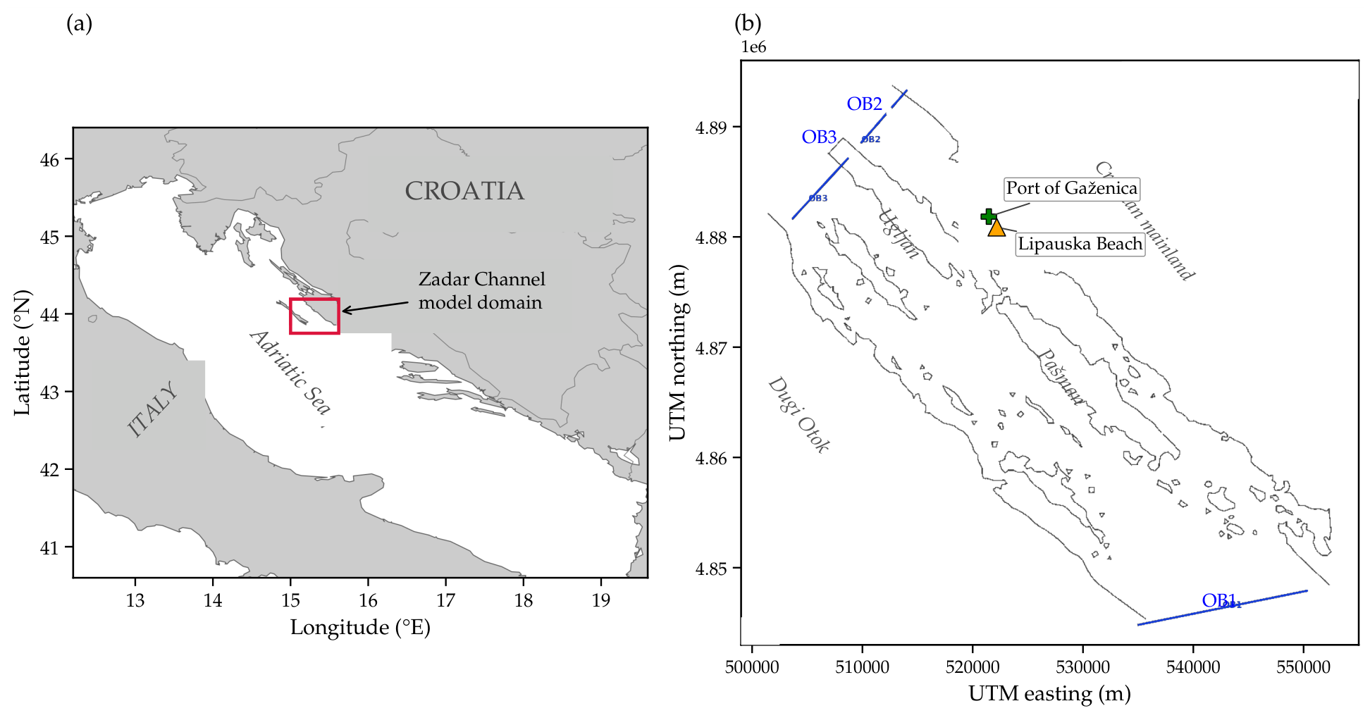
Figure 1 places the model domain within the Adriatic and then shows the computational boundaries and geographic reference points used throughout this paper.

The regional and projected views confirm that the Gaženica–Lipauska sector lies inside the domain and away from the three imposed open boundaries; the two labelled points are orientation markers rather than model source or receptor geometries.

The applied motivation is the movement of suspended or floating material near Zadar. Pier 3 at the cargo port of Gaženica provides a plausible bulk-cargo source scenario because it handles grain and other food cargoes and has a deep-water quay suitable for large vessels [7]. The present calculations do not simulate a measured spill or a specified mass release. A “particle” is a passive virtual particle used for Lagrangian transport calculations. It has no intrinsic mass, buoyancy, settling velocity, or material identity and follows the simulated velocity field plus prescribed horizontal diffusion, unless source-specific processes such as settling, windage, weathering, or Stokes drift are introduced. The results therefore diagnose pathways and numerical shoreline-contact tendencies of a virtual-particle ensemble rather than concentrations, deposition loads, or ecological effects.

A receptor is a place where transported material may matter. In the Gaženica application, the relevant receptors include the port mouth, near-source seabed, Lipauska Beach, Punta Bajlo, the Bibinje shoreline, and shallow benthic habitats. For a particulate application, the main receptor quantities are surface reach, shoreline contact, residence time, export through the port mouth, and deposition and vertical distribution. The source–pathway–receptor language separates three questions: where material enters the water, how the hydrodynamic field moves it, and where it may arrive. This study develops the chain’s channel-scale hydrodynamic and passive-particle components and defines metrics proposed for future Pier 3 source-polygon and receptor-exposure calculations. The event-window experiment uses $N_0=1000$ virtual particles as an ensemble sample of passive pathways under fixed hydrodynamic forcing, horizontal diffusivity, and shoreline rules. This number is a numerical sampling choice, not a representation of 1000 physical objects or a prescribed pollutant mass. The cumulative shoreline-contact fraction is $G\left(t\right)=N_g\left(t\right)/N_0$, where $N_g\left(t\right)$ is the number of particles that have met the explicit contact criterion by time t. With 1000 particles, one particle changes $G\left(t\right)$ by 0.001, or 0.1 percentage points.

The historical event considered is the 16–17 June 2025 Zadar storm. Official Croatian reports describe a severe storm that affected Zadar County on the evening of 16 June 2025, with maritime consequences in and near the Zadar Channel, including vessel groundings and the flooding of the passenger catamaran Melita; MRCC Rijeka reported more than 270 storm-related calls during the night [8,9,10]. The event provides a documented forcing period for testing current-driven passive-particle pathways under energetic meteorological forcing; it is not used here for meteorological attribution.

The scientific question is therefore as follows: for a geometrically complex Zadar Channel configuration, what channel-scale pathways and shoreline-contact tendencies are produced by the simulated hydrodynamic field, and how sensitive are those pathways to horizontal diffusivity and vertical layer?

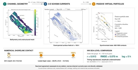
The contribution has four parts. First, the study documents a SCHISM circulation configuration for the Zadar Channel, including its unstructured horizontal and SZ vertical grids and its tidal and atmospheric forcing. Second, it evaluates the modelled free-surface response against independent hourly MP Zadar tide-gauge observations provided by the Hydrographic Institute of the Republic of Croatia (HHI). Third, it couples the simulated circulation to an offline unstructured-grid particle tracker and quantifies how horizontal stochastic spreading and the sampled model layer alter 24 h transport. Fourth, it links the event-period current field to cumulative shoreline contact for a 1000-particle ensemble. The methodological contribution is an integrated, reproducibly documented workflow; the regional finding is that vertical-layer selection changes passive reach more strongly than the tested variation in horizontal diffusivity, while the resolved channel current controls the dominant along-channel pathway.

This paper is organized as follows. Section 2 describes the computational domain and discretisation, hydrodynamic configuration, external forcing, observation-based free-surface validation, offline particle tracker, event-period design, and receptor metrics. Section 3 presents the hydrodynamic fields, passive-particle sensitivity tests, tide-gauge validation, Copernicus grid-coverage assessment, and synchronized event sequence. Section 4 interprets the process controls, defines the scope of the validation, and clarifies the passive-particle assumptions. Section 5 states the channel-scale findings and their observational limits.

2. Materials and Methods

The methods follow the numerical chain from physical space to reported transport quantities: horizontal and vertical discretisation, hydrodynamic equations and configuration, external forcing, observation-based free-surface validation, offline particle tracking, event-period simulation design and receptor metrics. This order separates the physical equations, SCHISM implementation choices, validation protocol, and Lagrangian post-processing.

2.1. Computational Domain and Discretisation

The computational domain covers the waters between Dugi Otok, Ugljan, Pašman, and the Croatian mainland near Zadar. Three open boundaries (Figure 1b) allow exchange with adjacent waters: one boundary in the south and two in the north. Coastlines and islands are treated as land boundaries. The source grid contains 63 land-boundary groups and 1223 land-boundary nodes.

All projected model maps use WGS 84/UTM zone 33N (EPSG:32633). The official Port of Gaženica reference coordinate, 44.08943° N, 15.26808° E [11], transforms to approximately 521,461 m easting and 4,881,841 m northing. The Lipauska marker uses an approximate publicly mapped beach-centre coordinate 44.0807232° N, 15.277038° E [12], or approximately 522,181 m easting and 4,880,876 m northing in the same CRS. These two markers are geographic references only; they do not define the diagnostic release point, a source polygon, or a receptor boundary.

As shown in Figure 1b, the Gaženica–Lipauska sector is located in the interior of the computational domain, away from the open boundaries. This placement minimizes the influence of boundary-forcing errors on the simulated particle dispersion in the study area. If a boundary were placed too close to the port or the beach, the imposed boundary condition could influence the pathways that should emerge from the hydrodynamic solution. Keeping the source and receptor areas within the domain helps separate local channel transport from boundary artefacts.

The domain is therefore larger than the immediate port–beach problem by design. This numerical setup keeps the source and receptor areas away from the open boundaries and allows the local particle cloud to evolve within the resolved channel geometry. In the 24 h tests reported below, the particle cloud remains in the local Zadar Channel sector under the tested conditions.

The same figure also explains why an unstructured grid is appropriate. The coastline follows long islands, narrow passages, small islands and bays. A structured rectangular grid would either smooth much of this geometry or require unnecessary resolution everywhere. Two mesh versions were developed during model construction: a coarse grid for preliminary technical tests and the adopted fine grid for the reported calculations. The adopted grid was selected to resolve channel-scale circulation and transport, not individual harbor structures. It preserves the principal island–mainland passages and large-scale coastline curvature at a computational cost compatible with the event calculation using the supplied 240-record atmospheric sequence.

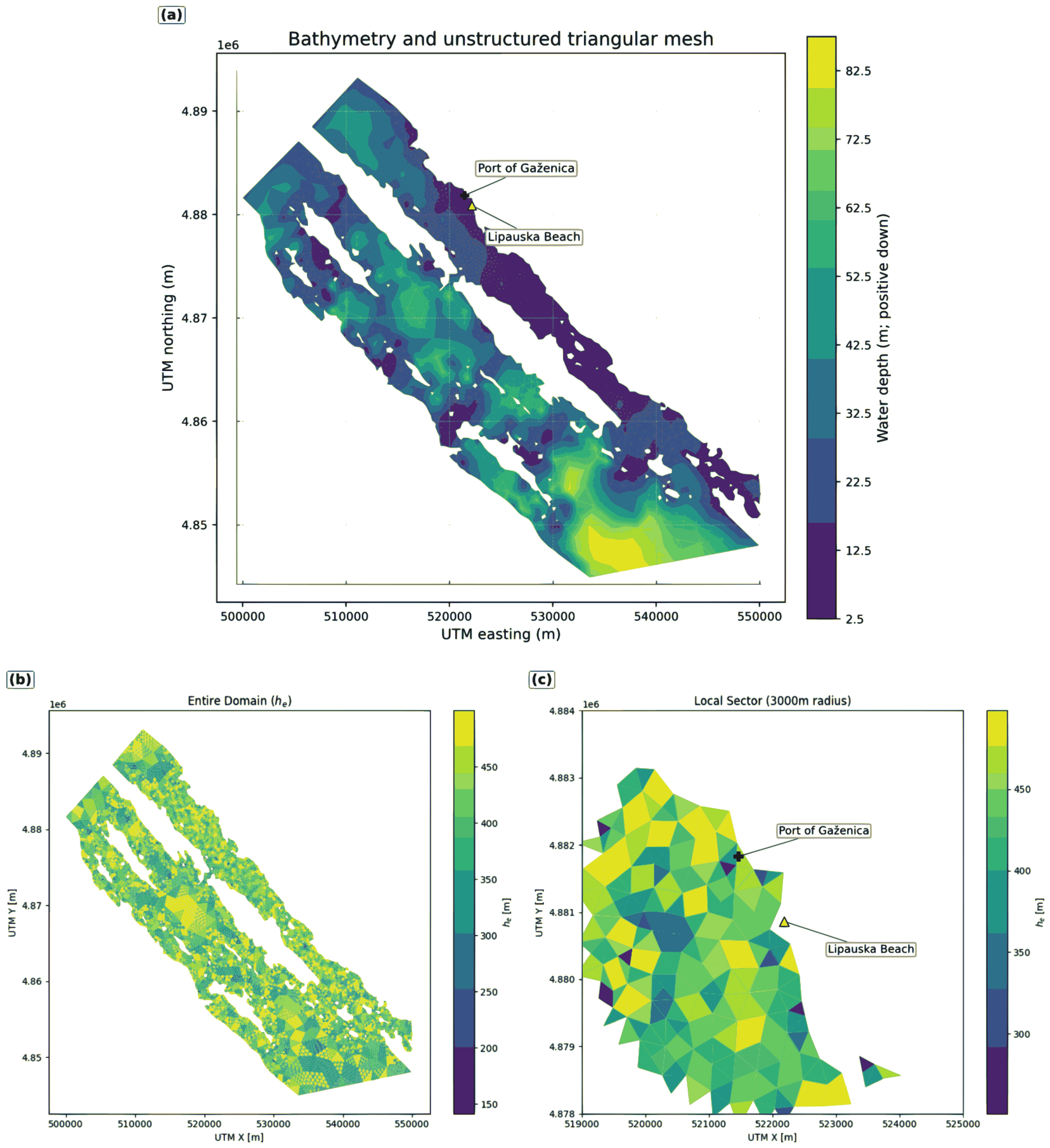
The mesh (hgrid.gr3) contains 16,962 triangular elements and 9081 nodes in projected UTM coordinates. Because one nominal value cannot describe an unstructured grid, the element-size metric is defined as $h_e=\max (l_{12},l_{23},l_{31})$, the longest edge of triangle e. Figure 2 and

Table 1. Element-size statistics based on $h_e=\max (l_{12},l_{23},l_{31})$. The local Gaženica–Lipauska sector is defined by a 3000 m radius around the sector centre.

Statistic	Entire Domain (m)	Gaženica–Lipauska Sector (m)
Minimum	141.51	279.81
Median	401.06	437.51
Mean	395.25	422.12
95th percentile	491.06	486.12
Maximum	499.91	490.81

show that $h_e$ ranges from 141.51 to 499.91 m over the full domain, with a median of 401.06 m. In the 3000 m Gaženica–Lipauska sector, the median is 437.51 m and the 95th percentile is 486.12 m. The local values therefore remain close to the nominal 500 m channel-scale design and do not imply harbor-scale resolution.

Bathymetric depths were obtained from the EMODnet Bathymetry Digital Terrain Model through the EMODnet web-coverage service [13]. The source DTM has a nominal spacing of $1/16\times 1/16$ arc minute, corresponding at the latitude of the Zadar Channel to approximately 115 m north–south and 80–85 m east–west. It is a harmonized composite of heterogeneous surveys and regional products, so one uniform vertical accuracy cannot be assigned to the entire domain. The raster depth field was interpolated to the unstructured SCHISM nodes; no additional bathymetric smoothing was applied after interpolation, and positive values in hgrid.gr3 denote water depth.

Figure 2 displays the bathymetry and the spatial distribution of the longest-edge element metric, while Table 1 provides the corresponding full-domain and local summary statistics.

Resolution implications. In the Gaženica–Lipauska sector, $h_e$ ranges from 279.81 to 490.81 m, with a median of 437.51 m. The grid resolves kilometre-scale passages and channel pathways, but not individual quays, breakwaters, beach morphology, harbor recirculation, or the thin nearshore shear layer. The finer EMODnet raster does not create hydrodynamic resolution below the SCHISM element scale. Port-specific exposure work therefore requires local refinement, higher-resolution nearshore bathymetry, and a formal coarse–baseline–fine convergence study.

Table 1 converts the mapped resolution field into the five statistics used to delimit the numerical scale of interpretation.

The local median and 95th-percentile values remain close to the nominal 500 m design, confirming that the adopted grid supports channel-scale interpretation but not harbor-scale claims.

A formal grid-convergence study was not completed. The available coarse grid was used only for preliminary setup tests and was not run with an otherwise identical forcing and diagnostics package, so a defensible coarse–baseline–fine convergence rate cannot be reported. Numerical stability and mass conservation are therefore not presented as evidence of grid independence. Peak water levels, local current magnitudes, and particle-reach metrics may contain discretisation-related uncertainty; the quantitative values in this paper should be interpreted at the resolution documented above.

2.2. Hydrodynamic Model Configuration

The hydrodynamic component computes sea currents with the Semi-implicit Cross-scale Hydroscience Integrated System Model (SCHISM), a semi-implicit unstructured-grid model for cross-scale hydroscience applications [14,15]. The free-surface continuity equation is

$${\displaystyle \frac{\partial \eta }{\partial t}}+{\displaystyle \frac{\partial \left(Hu\right)}{\partial x}}+{\displaystyle \frac{\partial \left(Hv\right)}{\partial y}}=0,$$

(1)

where $\eta$ is the free-surface elevation, $H=h+\eta$ is the total water depth, h is the bathymetric depth, and u and v are the horizontal velocity components in the x- and y-directions, respectively. The horizontal momentum equations are written as

$$\begin{array}{cc}\hfill {\displaystyle \frac{\partial u}{\partial t}}+u{\displaystyle \frac{\partial u}{\partial x}}+v{\displaystyle \frac{\partial u}{\partial y}}+w{\displaystyle \frac{\partial u}{\partial z}}-fv& =-g{\displaystyle \frac{\partial \eta }{\partial x}}+{\displaystyle \frac{\partial }{\partial z}}\left(\nu {\displaystyle \frac{\partial u}{\partial z}}\right)+F_u,\hfill \end{array}$$

(2)

$$\begin{array}{cc}\hfill {\displaystyle \frac{\partial v}{\partial t}}+u{\displaystyle \frac{\partial v}{\partial x}}+v{\displaystyle \frac{\partial v}{\partial y}}+w{\displaystyle \frac{\partial v}{\partial z}}+fu& =-g{\displaystyle \frac{\partial \eta }{\partial y}}+{\displaystyle \frac{\partial }{\partial z}}\left(\nu {\displaystyle \frac{\partial v}{\partial z}}\right)+F_v.\hfill \end{array}$$

(3)

Here, w is the vertical velocity, f is the Coriolis parameter, g is the gravitational acceleration, $\nu$ is the vertical viscosity, and $F_u$ and $F_v$ are the horizontal diffusion terms in the x- and y-directions, respectively.

Equation (1) expresses conservation of water volume, whereas Equations (2) and (3) represent the balance between acceleration, the pressure-gradient force, the Coriolis force, vertical mixing, and horizontal diffusion. These equations state the physical problem. The numerical implementation is described separately: the SCHISM/SELFE model family combines semi-implicit finite elements for hydrodynamics with a finite-volume treatment of transport. In the present configuration, the hydrodynamic run is barotropic (ibc = 0), vertical mixing is represented by a two-equation generic-length-scale turbulence closure (itur = 2), the Coriolis parameter is held constant (ncor = 0), and explicit horizontal diffusion is disabled (ihdif = 0). Executable and run-control details are reported in

Table 2. Core configuration of the Zadar Channel hydrodynamic implementation.

Item	Configured Value
Model	SCHISM three-dimensional hydrostatic shallow-water model; barotropic setup (ibc = 0).
Domain and boundaries	Dugi Otok–Ugljan–Pašman–mainland channel system; 3 open boundaries and 63 land-boundary groups.
Horizontal mesh	16,962 triangular elements and 9081 nodes. Median $h_e$ is 401.06 m domain-wide and 437.51 m in the 3000 m Gaženica–Lipauska sector; full statistics are given in Table 1.
Vertical grid	SZ vertical coordinate, 20 levels, ivcor = 2, kz = 1, hs = 100 m, hc = 30 m, ${\theta }_b=0.7$, ${\theta }_f=10.0$.
Time control	Hydrodynamic time step $\Delta t=60$ s; 1 d forcing ramp; NetCDF output every 30 model steps (30 min).
Initial state	Zero velocity and free-surface elevation; uniform 10 °C temperature and 35 PSU salinity.
Numerics	Semi-implicit time stepping (${\theta }_i=0.8$), Manning bottom friction ($n=0.025$ s m−1/3), GLS turbulence option (itur = 2), constant Coriolis (ncor = 0), explicit horizontal diffusion disabled (ihdif = 0).
Execution	MPI test runs with 2–6 processors using the pschism_TVD-VL executable.

.

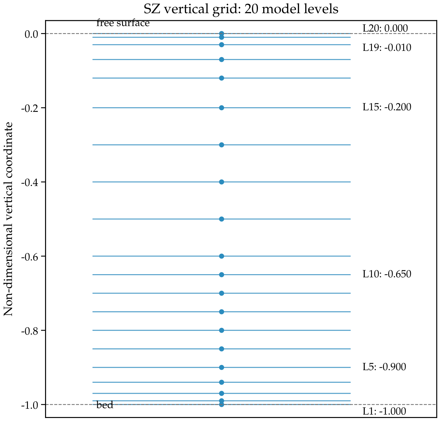
Table 2 condenses the model setup into the values needed to reproduce the diagnostic run. The documented diagnostic configuration began at 12:00 UTC on 1 January 2000 and ran for 4 days; shorter integrations were used only during preliminary technical testing. The vertical grid uses the SZ option with 20 levels and clustering near the bed and the free surface, consistent with the flexible vertical-coordinate approach developed for unstructured-grid coastal models [16].

Table 2 separates the hydrodynamic run controls from the particle-tracker controls reported later; in particular, the 60 s SCHISM time step and 30 min output interval are not the particle integration step.

Figure 3 shows how the 20 model levels are distributed between the bed and the free surface.

Figure 3 shows enhanced resolution near both the bed and the free surface. Because the horizontal velocity varies with depth, the vertical level from which a particle is advected determines the currents it samples, and hence the simulated trajectory and 24 h reach. The layer index is therefore reported explicitly: the surface diagnostic tests use L19 and the lower-layer sensitivity test uses L15, so the same horizontal release point samples different velocities depending on the level.

2.3. Tidal, Atmospheric and Initial Forcing

The external forcing provides the boundary and surface conditions from which the hydrodynamic field is calculated. Open-boundary water levels use the M2 and K1 constituents, specified in the bctides.in file with tidal potential disabled (ntip = 0) and a nodal factor of unity. M2 has a period of approximately 12.42 h and K1 approximately 23.93 h. Free-surface elevation is prescribed at all three open boundaries from the constituent amplitudes and phases reported in Table 3. At the southern boundary, normal-velocity harmonics are additionally imposed (M2: 0.10 m s⁻¹ at 310°; K1: 0.05 m s⁻¹ at 330°); no regional velocity product is imposed. The interior current field therefore evolves from the specified boundary elevations and southern-boundary velocity harmonics together with atmospheric forcing, local bathymetry, coastline geometry, bottom friction, and mass conservation. During the analyzed period, the prescribed elevation difference between the southern and northern open boundaries reached approximately 0.07 m, providing a barotropic pressure-gradient contribution to exchange through the island-channel system.

Table 3. Tidal and atmospheric forcing in the diagnostic and June 2025 event configurations.

Forcing Element	Configured Value
Open boundaries	101 total open-boundary nodes: southern boundary (57 nodes), northwestern boundary (29 nodes), and northeastern boundary (15 nodes).
Tidal elevation	M2 and K1 elevation prescribed at all three open boundaries. Southern boundary: M2 0.180 m at 310° and K1 0.090 m at 330°. Northwestern and northeastern boundaries: M2 0.120 m at 295° and K1 0.060 m at 315°.
Boundary velocity	Southern-boundary normal-velocity harmonics: M2 0.10 m s−1 at 310° and K1 0.05 m s−1 at 330°. No velocity harmonics are imposed at the two northern boundaries, and no regional velocity field is prescribed.
Diagnostic atmosphere	Earlier diagnostic tests used the documented $17\times 17$ local ERA5-derived cut-out, sampled every 3 h with approximate 3 km horizontal spacing.
Event-period atmosphere	ERA5-derived SCHISM sflux grid with $81\times 81$ points, $0.05°\times 0.05°$ spacing, covering 12–16° E and 43–47° N. Mean neighbor spacing is approximately 3.93 km east–west and 5.56 km north–south.
Event-window temporal coverage	240 nominally hourly records covering 10–19 June 2025 (10 June 00:00 UTC through 19 June 23:00 UTC); displayed analyses extend through $t=192$ h.
Interpolation note	The 0.05° sflux grid is a spatial interpolation of the source ERA5 fields and does not increase the intrinsic information content of the reanalysis.
Closed boundaries	Coastline, islands, and mainland treated as impermeable land boundaries; the particle tracker applies the explicit shoreline and wet–dry rules in Table 4.

Table 3. Tidal and atmospheric forcing in the diagnostic and June 2025 event configurations.

Forcing Element	Configured Value
Open boundaries	101 total open-boundary nodes: southern boundary (57 nodes), northwestern boundary (29 nodes), and northeastern boundary (15 nodes).
Tidal elevation	M2 and K1 elevation prescribed at all three open boundaries. Southern boundary: M2 0.180 m at 310° and K1 0.090 m at 330°. Northwestern and northeastern boundaries: M2 0.120 m at 295° and K1 0.060 m at 315°.
Boundary velocity	Southern-boundary normal-velocity harmonics: M2 0.10 m s−1 at 310° and K1 0.05 m s−1 at 330°. No velocity harmonics are imposed at the two northern boundaries, and no regional velocity field is prescribed.
Diagnostic atmosphere	Earlier diagnostic tests used the documented $17\times 17$ local ERA5-derived cut-out, sampled every 3 h with approximate 3 km horizontal spacing.
Event-period atmosphere	ERA5-derived SCHISM sflux grid with $81\times 81$ points, $0.05°\times 0.05°$ spacing, covering 12–16° E and 43–47° N. Mean neighbor spacing is approximately 3.93 km east–west and 5.56 km north–south.
Event-window temporal coverage	240 nominally hourly records covering 10–19 June 2025 (10 June 00:00 UTC through 19 June 23:00 UTC); displayed analyses extend through $t=192$ h.
Interpolation note	The 0.05° sflux grid is a spatial interpolation of the source ERA5 fields and does not increase the intrinsic information content of the reanalysis.
Closed boundaries	Coastline, islands, and mainland treated as impermeable land boundaries; the particle tracker applies the explicit shoreline and wet–dry rules in Table 4.

Table 4. Particle-tracker metadata for the June 2025 passive-drift event calculation.

Parameter	Configured Value
Ensemble and release	1000 particles released simultaneously at $t=0$; no subsequent release.
Initial cloud	Independent Gaussian offsets about the source, with standard deviation 20 m in both horizontal directions.
Random-number control	NumPy default_rng; fixed seed 42.
Velocity sampling	SCHISM surface layer (layer $=-1$); hydrodynamic fields available every 30 min.
Particle time step	Four substeps per hydrodynamic output interval, giving $\Delta t_p=450$ s (7.5 min).
Horizontal diffusion	Constant random-walk diffusivity $K_h=0.5$ m2 s−1 for the event calculation.
Shoreline rule	Permanent numerical shoreline contact when an active particle comes within 50 m of the model shoreline; the particle is then removed from further transport.
Wet–dry handling	Moves ending outside the wet domain, or line segments intersecting a shoreline boundary, are rejected and rolled back to the last valid wet position.
Counting rule	Each particle is counted once, at its first shoreline-contact event; reported counts are cumulative unique particle contacts.

Table 4. Particle-tracker metadata for the June 2025 passive-drift event calculation.

Parameter	Configured Value
Ensemble and release	1000 particles released simultaneously at $t=0$; no subsequent release.
Initial cloud	Independent Gaussian offsets about the source, with standard deviation 20 m in both horizontal directions.
Random-number control	NumPy default_rng; fixed seed 42.
Velocity sampling	SCHISM surface layer (layer $=-1$); hydrodynamic fields available every 30 min.
Particle time step	Four substeps per hydrodynamic output interval, giving $\Delta t_p=450$ s (7.5 min).
Horizontal diffusion	Constant random-walk diffusivity $K_h=0.5$ m2 s−1 for the event calculation.
Shoreline rule	Permanent numerical shoreline contact when an active particle comes within 50 m of the model shoreline; the particle is then removed from further transport.
Wet–dry handling	Moves ending outside the wet domain, or line segments intersecting a shoreline boundary, are rejected and rolled back to the last valid wet position.
Counting rule	Each particle is counted once, at its first shoreline-contact event; reported counts are cumulative unique particle contacts.

The diagnostic and event-period experiments use different atmospheric files and are reported separately. The earlier diagnostic tests used the documented $17\times 17$ local ERA5-derived cut-out sampled every 3 h, with an approximate physical spacing of 3 km in both horizontal directions. The June 2025 event calculation used SCHISM surface-flux (sflux) NetCDF files containing the eastward and northward components of 10 m wind, mean sea-level pressure, 2 m air temperature, and specific humidity [17]. Coordinates extracted from the event file define an $81\times 81$ grid covering 12–16° E and 43–47° N, with increments of 0.05° in both directions. Great-circle distances between adjacent coordinates correspond to mean spacings of approximately 3.93 km east–west and 5.56 km north–south. The file contains 240 nominally hourly records covering the ten calendar days from 10 June 2025 00:00 UTC through 19 June 2025 23:00 UTC. The displayed analyses extend through $t=192$ h, within this forcing-record sequence. The 0.05° grid is an interpolation of the source ERA5 fields and does not represent increased native information content. This interpretation is consistent with an eastern Adriatic JMSE assessment showing that ERA5 forcing in fetch-limited basins must be evaluated against local observations rather than treated as a locally resolving wind product [18].

The base_date attribute of the ERA5-derived NetCDF files was reformatted from a character string to the integer array expected by SCHISM, and the model start time was aligned with the forcing time origin. The diagnostic run starts from zero velocity and free-surface elevation with uniform 10 °C temperature and 35 PSU salinity.

Table 3 summarizes the boundary conditions and keeps the diagnostic and event-period atmospheric files explicitly separate.

The table makes clear that only the June 2025 event uses the 81 × 81 hourly forcing file; the earlier 17 × 17, 3 h file belongs to the diagnostic configuration.

2.4. Observation-Based Free-Surface Validation

Hydrodynamic model performance was evaluated using independent hourly sea-level observations from the MP Zadar (ZD0) tide-gauge station operated by HHI [19]. The station is located at 44.119160° N, 15.230394° E. Sea level was extracted at the nearest wet SCHISM computational node, approximately 505 m from the gauge, where the model water depth is 16.59 m. This separation is comparable to one local mesh-element width but substantially smaller than the approximately 4 km Copernicus grid spacing. Together with the weaker small-scale spatial variability of sea level than of current velocity, it makes the tide-gauge record more suitable for quantitative assessment of the modelled free-surface response than the regional velocity product.

Observed and simulated sea levels were compared over their common temporal interval within 10–19 June 2025. The HHI station page reports station time as UTC+1; the observation timestamps were therefore expressed in UTC before matching to model time. Exact SCHISM outputs coincident with the observation hours were selected from the 30 min model-output sequence. The first 24 h of the SCHISM simulation were excluded to avoid the documented one-day forcing-ramp period. Retaining timestamps available in both post-ramp series produced 192 hourly model–observation pairs. The HHI observations were not used to tune the tidal boundary amplitudes or phases. No temporal shift or fitted constant vertical offset was applied to either series for the primary comparison.

The observed values were expressed relative to the station reference level supplied with the HHI record, and the model values relative to the SCHISM vertical reference. Accordingly, the reported bias quantifies the mean difference between those supplied series over the matched interval; it is not a geodetic comparison of the two vertical datums. The separately demeaned analysis described below isolates temporal co-variability from any constant reference-level difference.

Let ${\eta }_{m,i}$ and ${\eta }_{o,i}$ denote the modelled and observed sea levels at matched hour i, and let $e_i={\eta }_{m,i}-{\eta }_{o,i}$. Model performance was summarized by mean bias, mean absolute error (MAE), root-mean-square error (RMSE), and the Pearson correlation coefficient:

$$\begin{array}{cccc}\hfill \mathrm{Bias}& ={\displaystyle \frac{1}{N}}{\displaystyle \sum _{i=1}^N}{e}_i,\hfill & \hfill \mathrm{MAE}& ={\displaystyle \frac{1}{N}}{\displaystyle \sum _{i=1}^N}\left|e_i\right|,\hfill \end{array}$$

(4)

$$\begin{array}{cccc}\hfill \mathrm{RMSE}& =\sqrt{{\displaystyle \frac{1}{N}}\sum _{i=1}^N{e}_i^2}.\hfill & & \end{array}$$

(5)

Because the absolute reference levels of the observed and modelled series need not be identical, their standard deviations and the RMSE of the separately demeaned series were also examined. Cross-correlation of the demeaned series over integer-hour lags was used as a diagnostic test for a systematic temporal offset; the lag analysis did not alter the timestamps used for the primary statistics. The temporal resolution of this test is 1 h and therefore cannot exclude a sub-hour phase difference. These skill measures are descriptive summaries of one autocorrelated hourly record, and no independent-sample significance claim is attached to them.

2.5. Offline Lagrangian Particle Tracking

The particle tracker is run offline using hydrodynamic NetCDF outputs and follows the physical principles of the SCHISM PTRACK4 module. A particle denotes a passive conservative virtual particle transported by the simulated current and prescribed horizontal diffusion; it has no intrinsic physical properties unless source-specific terms are introduced. Horizontal velocity components are read as horizontalVelX and horizontalVelY; barycentric interpolation inside triangular elements provides velocity at each particle position [20].

The deterministic step uses a second-order Heun scheme,

$$\begin{array}{cc}\hfill {\mathit{x}}^{\ast }& ={\mathit{x}}^n+\Delta t_p\mathit{u}({\mathit{x}}^n,t^n),\hfill \end{array}$$

(6)

$$\begin{array}{cc}\hfill {\mathit{x}}^{n+1}& ={\mathit{x}}^n+{\displaystyle \frac{\Delta t_p}{2}}\left[\mathit{u}({\mathit{x}}^n,t^n)+\mathit{u}({\mathit{x}}^{\ast },t^{n+1})\right],\hfill \end{array}$$

(7)

where ${\mathit{x}}^n$ is the particle position at time $t^n$, ${\mathit{x}}^{\ast }$ is the predictor position, $\Delta t_p$ is the particle time step, and $\mathit{u}$ is the interpolated horizontal velocity. Unresolved horizontal spreading is represented by a constant-diffusivity random walk [21],

$$\Delta {\mathit{x}}_d=\sqrt{2K_h\Delta t_p}\mathit{R},$$

(8)

where $\mathit{R}$ contains independent standard normal variates.

For the June 2025 event calculation, 1000 particles were released simultaneously at $t=0$ and no particles were added later. Initial positions were sampled from independent Gaussian distributions centred on the source with a standard deviation of 20 m in both horizontal directions. A fixed NumPy default_rng seed of 42 controls both the initial cloud and stochastic displacement. The surface-layer velocity fields (layer $=-1$) were available every 30 min, and each interval was divided into four substeps, giving $\Delta t_p=450$ s. The event calculation uses $K_h=0.5$ m² s⁻¹.

Shoreline interaction is represented by a permanent numerical contact rule (“hard contact”). At each substep, an active particle that comes within 50 m of the model shoreline is classified as contacted, returned to its last valid wet position, and removed from subsequent advection and random-walk updates. Moves that end outside the wet domain, and trajectory segments that cross a shoreline boundary, are rejected and rolled back. Each particle is counted once, at first contact, so the reported values are cumulative counts of unique particle shoreline contacts. This rule is a model diagnostic and should not be interpreted as a physical deposition, adhesion, or resuspension model.

Table 4 consolidates the ensemble, time-stepping, diffusion, and shoreline-contact choices needed to reproduce the event calculation.

The reported trajectories therefore combine SCHISM-current advection and the stochastic term in Equation (8). They do not include settling, deposition, resuspension, flocculation, direct windage, or Stokes drift. Those processes require particle-class-specific parameters and, for Stokes drift, wave-model fields; none is inferred from the passive-particle results.

2.6. June 2025 Event-Window Simulation Design

The event-window calculation begins on 10 June 2025 and uses the supplied 240-record atmospheric sequence. M2 and K1 tidal forcing is applied throughout, together with hourly ERA5-derived wind, sea-level pressure, air temperature, and humidity [22]. The initial part of the integration provides model spin-up, the night of 16–17 June contains the documented maritime emergency conditions, and the later part of the available record covers post-event evolution. The synchronized figures report selected states through $t=192$ h, within the available forcing record. The particles are released at the beginning of the 10 June integration rather than at storm onset. The displayed sequence must therefore be interpreted as a passive-transport experiment spanning the pre-event, event, and post-event periods, not as a causal estimate of transport generated solely by the 16–17 June storm. The source location, 1000-particle ensemble, random seed, $K_h$, particle time step, and shoreline-contact rule remain fixed, so differences among the displayed states arise from the time-varying hydrodynamic field and the single reproducible stochastic realization. The experiment does not model meteorological causation or the fate of a specified particulate class.

The Copernicus Global Ocean Waves Analysis and Forecast product based on MFWAM provides wave parameters and Stokes-drift components on a $1/12°$ grid [23]. Direct interpolation of those vectors into the sub-kilometre island passages would not resolve shoreline sheltering or local wave transformation. SCHISM’s WWM component could instead use regional wave-boundary conditions and wind forcing to calculate a locally transformed wave field. WWM was not activated in the present experiment, and neither wave–current feedback nor Stokes drift is included. Their effect is therefore unquantified, and no claim is made that wave-induced transport was negligible. The trajectories reported here are explicitly the current-driven reference case.

2.7. Port-Particulate and Receptor Metrics

The implemented cases treat the released objects as passive virtual particles, which provide the hydrodynamic reference case for particulate transport. The present calculations do not instantiate material classes. A future Gaženica application would distinguish five source-specific classes: fine suspended dust or mineral–organic particles, slowly settling grain or husk fragments, dense mineral–organic aggregates, floating or near-surface organic fragments, and finite-size non-spherical particles. Representing these classes would require class-dependent density, size, shape, settling velocity, bed interaction, windage, and, where relevant, Stokes-drift parameterisation. The class distinction is essential because particle density, shape, and response time can make real particles depart from passive-drifter behavior [24]. The same receptor framework also accommodates shoreline contact and beaching diagnostics used in Lagrangian marine-litter source–distribution studies [6].

For the sensitivity experiments, maximum reach at time T is measured from the release position ${\mathit{x}}_0$ as

$$R_{\max }\left(T\right)=\underset{i}{\max }∥{\mathit{x}}_i\left(T\right)-{\mathit{x}}_0∥.$$

(9)

For a two-dimensional constant-diffusivity random walk, the characteristic root-mean-square spreading scale over time T is

$${\sigma }_d\left(T\right)=\sqrt{4K_{h}T}.$$

(10)

The event-window sequence is summarized by the cumulative shoreline-contact fraction

$$G\left(t\right)={\displaystyle \frac{N_g\left(t\right)}{N_0}},$$

(11)

where $N_g\left(t\right)$ is the number of particles that have contacted the wet–dry shoreline mask by time t. With $N_0=1000$, the empirical increment of G is 0.001 per particle.

For a receptor polygon ${\Omega }_r$, the contact probability over a time window T is

$$P_r\left(T\right)={\displaystyle \frac{1}{N_0}}{\displaystyle \sum _{i=1}^{N_0}}\mathbb{I}\left[{\mathit{x}}_i\left(t\right)\in {\Omega }_r\mathrm{for}\mathrm{some}0<t<T\right],$$

(12)

where ${\mathit{x}}_i\left(t\right)$ is the position of particle i, $N_0$ is the number of released particles, and $\mathbb{I}$ is the indicator function. A port-mouth export fraction can be written as

$$F_{\mathrm{out}}\left(T\right)={\displaystyle \frac{N_{\mathrm{out}}\left(T\right)}{N_0}},$$

(13)

where $N_{\mathrm{out}}$ is the number of particles crossing the port-mouth section outward. The residence-time survival function inside a basin or receptor polygon is

$$S\left(t\right)={\displaystyle \frac{N_{\mathrm{in}}\left(t\right)}{N_0}},$$

(14)

where $N_{\mathrm{in}}\left(t\right)$ is the number of particles remaining in the selected polygon. Equations (12)–(14) define the proposed first receptor outputs for source-specific Pier 3 particulate releases. These outputs can be complemented by shoreline-contact duration and, where deposition is included, by the mass or area remaining in each receptor polygon.

3. Results

3.1. Hydrodynamic Implementation and Output Fields

The configuration completed the reported integrations without input-file failure or detected numerical instability, and continuity/mass-balance diagnostics were monitored. These checks verify execution, not accuracy, grid convergence, or observational skill. The Manning roughness, TVD flux-limiter, initial-temperature, and initial-salinity fields were generated through purpose-written pre-processing scripts.

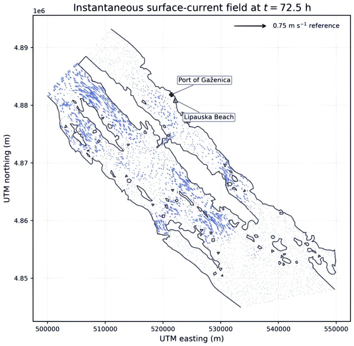
Figure 4 shows the surface-current field at $t=72.5$ h. Vectors follow the elongated island–mainland passages, strengthen in constrictions and weaken or vary in wider embayments; in the Gaženica–Lipauska sector, they align with the mainland–island channel. The plot is a model-output diagnostic, not observational validation. No direct current observations are available inside the narrow modelled passages for quantitative validation. As shown in Section 3.4, the nearest regional Copernicus product does not contain valid sea cells within those passages; its current field is therefore used only to describe surrounding regional circulation.

The snapshot confirms that island–mainland geometry organizes the advective field sampled by the particle tracker. It demonstrates internal process consistency but does not establish observational skill.

3.2. Passive-Particle Dispersion and Sensitivity

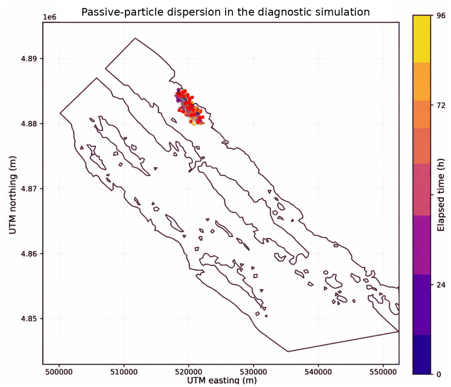
The diagnostic transport calculations release passive particles from a representative Zadar Channel source point identified in the model documentation as node ID 645. These trajectories form the passive horizontal transport reference case. Figure 5 is shown before the numerical sensitivity table, because the map explains what the maximum-reach values summarize.

Figure 5 shows an elongated advective pathway with lateral spreading around it. Because the particles are released from a representative channel node rather than a resolved port-source polygon, the cloud characterizes the diagnostic transport behavior of the channel and should not be interpreted as a prediction for a specific cargo release.

The diagnostic cloud should also be interpreted against the model extent. Although the grid includes Dugi Otok and the outer island-channel system, the diagnostic trajectories remain local within the Zadar Channel sector. The larger grid is retained to prevent boundary artefacts and to accommodate event-period simulations such as the June 2025 calculation.

Table 5. Twenty-four-hour passive-particle sensitivity and derived two-dimensional diffusive scales. $\Delta R$ is relative to Case A and ${\sigma }_d=\sqrt{4K_{h}T}$ with $T=24$ h.

Case	${\mathit{K}}_{\mathit{h}}$ (m2 s$-1$)	Layer	${\mathit{R}}_{\max }$ (km)	$\mathbf{\Delta }\mathit{R}$ (%)	${\mathit{\sigma }}_{\mathit{d}}$ (km)	${\mathit{R}}_{\max }/{\mathit{\sigma }}_{\mathit{d}}$
A	0.5	L19	12.5	0.0	0.416	30.1
B	1.5	L19	14.2	+13.6	0.720	19.7
C	0.1	L19	11.8	−5.6	0.186	63.4
D	0.5	L15 (lower layer)	8.4	−32.8	0.416	20.2

gives the four documented sensitivity cases. The table is placed immediately after the trajectory map so that the reader can connect the visual plume behavior with changes in horizontal diffusivity and vertical layer.

The sensitivity pattern is internally consistent with the implemented advection–diffusion framework. Increasing $K_h$ from 0.5 to 1.5 m² s⁻¹ increases the maximum 24 h reach from 12.5 to 14.2 km ($+13.6\%$) and broadens the particle cloud. Reducing $K_h$ to 0.1 m² s⁻¹ keeps the plume narrow and changes maximum reach by only $-5.6\%$, to 11.8 km. The derived two-dimensional spreading scales are 0.186–0.720 km, whereas the corresponding maximum reaches are 8.4–14.2 km; $R_{\max }/{\sigma }_d$ ranges from 19.7 to 63.4. These ratios show that the resolved current controls the longitudinal excursion and the stochastic term primarily controls lateral broadening. Moving the diagnostic particles from surface layer L19 to lower layer L15 reduces the 24 h reach from 12.5 to 8.4 km ($-32.8\%$), the largest tested change. Because SZ layer indices do not represent a fixed physical depth throughout the domain, L15 is reported by index rather than assigned a single nominal depth. The result is consistent with vertical shear and slower lower-layer velocities: the surface layer is more directly energized by wind stress and pressure gradients, whereas bottom friction slows the deeper layers.

3.3. Free-Surface Validation Against the MP Zadar Tide Gauge

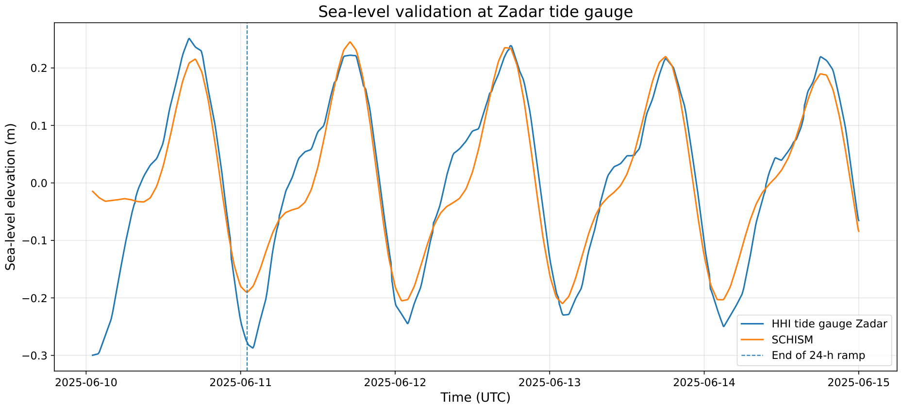
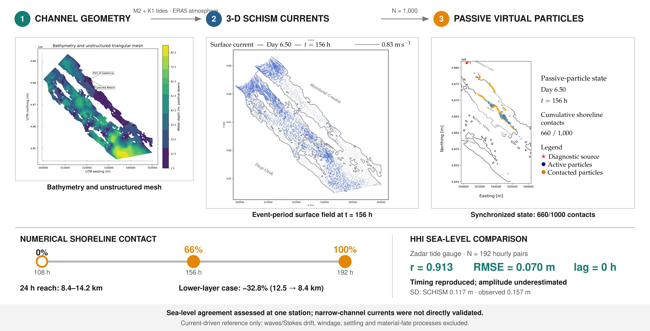
After exclusion of the first 24 h ramping period and matching of the common timestamps, 192 hourly observation–model pairs were available. The unshifted simulated and measured series were strongly correlated ($r=0.913$), with a mean bias of 0.012 m, an MAE of 0.051 m, and an RMSE of 0.070 m (Figure 6;

Table 6. Validation of simulated sea level against independent hourly observations at the MP Zadar tide gauge. Bias is defined as SCHISM minus HHI. The primary statistics use the matched series after exclusion of the first 24 h ramping period; no fitted temporal or vertical offset was applied.

Metric	SCHISM vs. HHI
Number of hourly pairs	192
Mean bias	0.012 m
Mean absolute error (MAE)	0.051 m
Root-mean-square error (RMSE)	0.070 m
Centred RMSE (series separately demeaned)	0.069 m
Pearson correlation	0.913
Optimal integer-hour lag	0 h
Correlation at optimal lag	0.913
HHI standard deviation	0.157 m
SCHISM standard deviation	0.117 m
Standard-deviation ratio (SCHISM/HHI)	0.745

).

Cross-correlation analysis identified an optimal integer-hour lag of 0 h, at which the correlation remained $r=0.913$. Thus, no temporal displacement of either series was required to obtain the reported agreement. The corresponding RMSE after separately demeaning the observed and modelled series was 0.069 m.

The principal discrepancy concerned amplitude. The standard deviation was 0.117 m for SCHISM and 0.157 m for the HHI observations, giving a model-to-observation standard-deviation ratio of 0.745. Thus, the simulated standard deviation was 74.5% of the observed value. The model reproduced the timing and temporal evolution of the observed oscillations but underestimated their magnitude.

3.4. Copernicus Grid Coverage and Representativeness

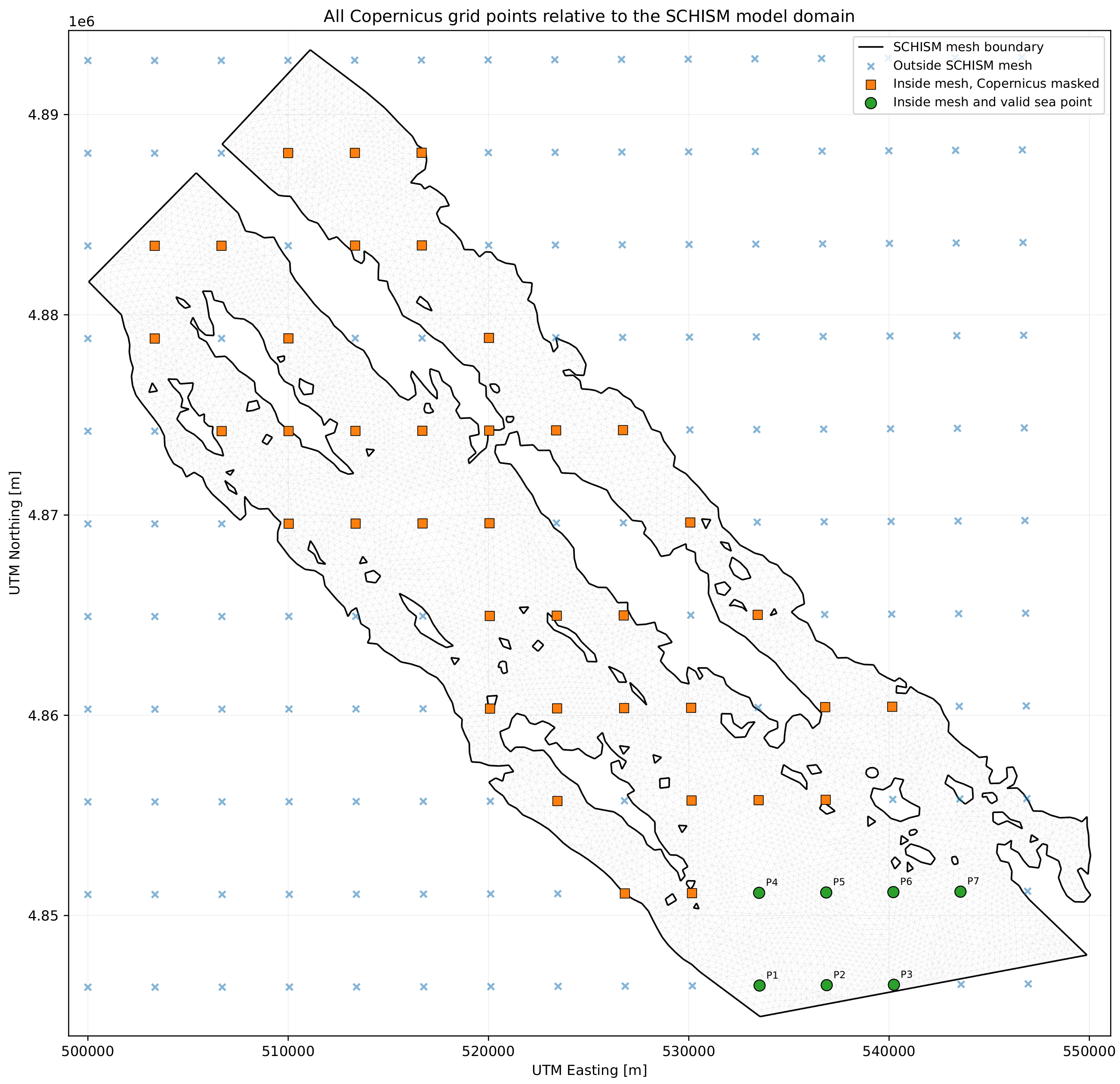
The Copernicus Marine Mediterranean Sea Physics Analysis and Forecast product [25] has approximately 4 km ($1/24°$) horizontal spacing and is designed for regional circulation. Every Copernicus grid centre within and around the SCHISM boundary was classified against the SCHISM coastline, and the validity mask was checked throughout the complete event interval. Figure 7 distinguishes points outside the SCHISM domain, points that lie inside the domain but are masked by Copernicus, and points that are valid sea cells in both products. The set of valid cells was invariant over the examined interval: the interior island passages in which the reported transport develops remained classified as land or masked cells, while only seven valid Copernicus sea points (P1–P7) occurred along the southern offshore edge of the SCHISM domain.

A comparison with the Copernicus regional current product was initially explored. However, the available offshore cells do not sample the hydraulically constrained channel interior, and the corresponding SCHISM and Copernicus velocity series agree poorly in timing and direction. The point-to-point statistics are therefore not presented as evidence of model skill. The comparison is retained only to demonstrate why the regional product is not spatially representative of the channel-scale velocity field.

The availability of HF-radar observations was also investigated. The operational HFR-NAdr network is located in the Gulf of Trieste, with a documented maximum radial coverage of approximately 35–40 km, and does not extend to the Zadar Channel [26]. No HF-radar dataset providing event-period coverage of the present model domain was identified. Consequently, HF-radar velocities could not be used for direct validation of this simulation; such validation would require measurements from an acoustic Doppler current profiler (ADCP), drifters, or equivalent instruments collected within the modelled passages.

The independent HHI tide-gauge comparison in Section 3.3 replaces the regional velocity comparison as the quantitative observational assessment of the modelled free-surface response. The change of validation variable is deliberate: sea level is substantially less sensitive than current velocity to the unresolved small-scale geometry separating the regional and channel-scale grids. The distinct limits of free-surface and current validation are addressed in Section 4.3.

3.5. June 2025 Event-Window: Synchronized Current–Particle Sequence

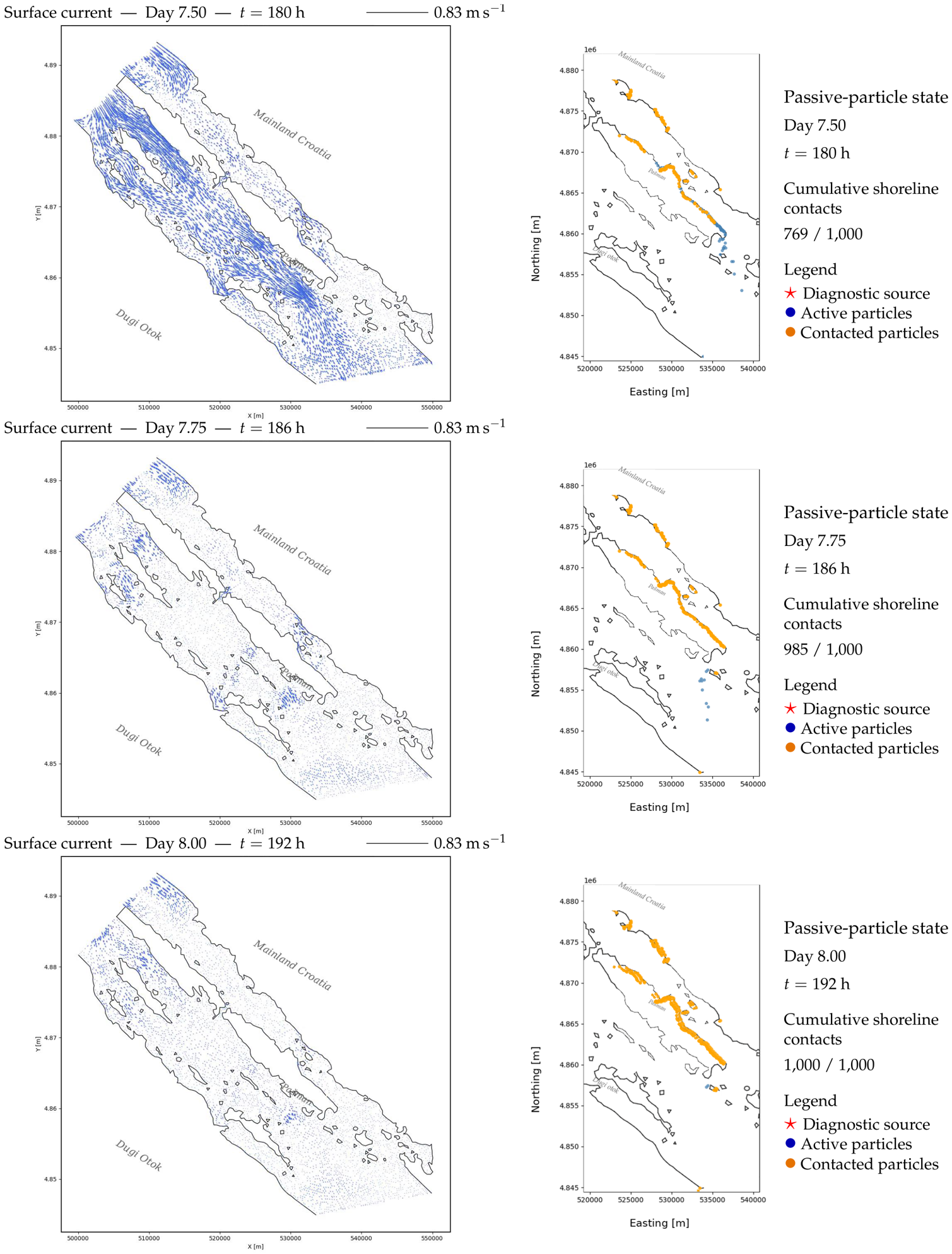
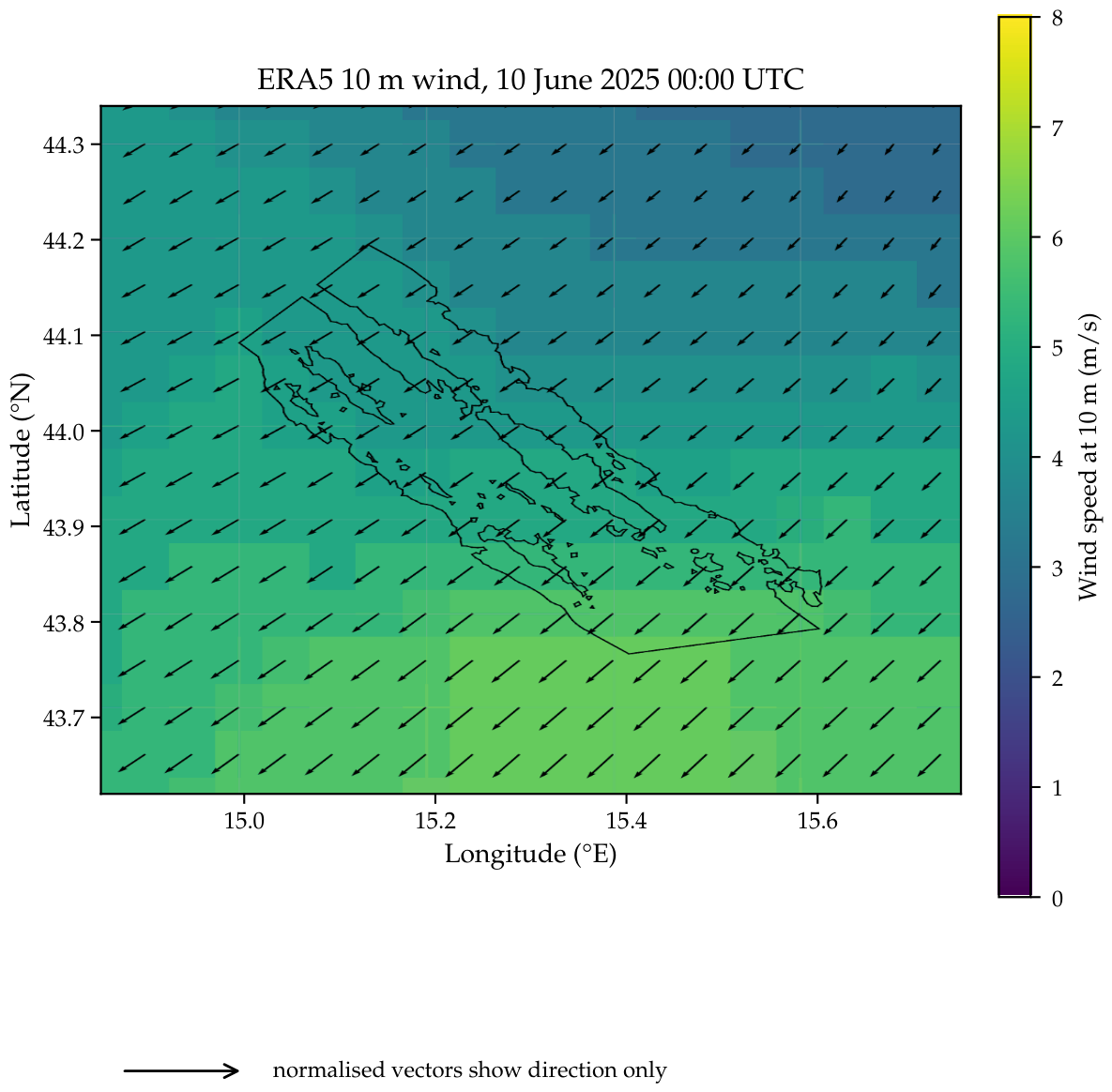
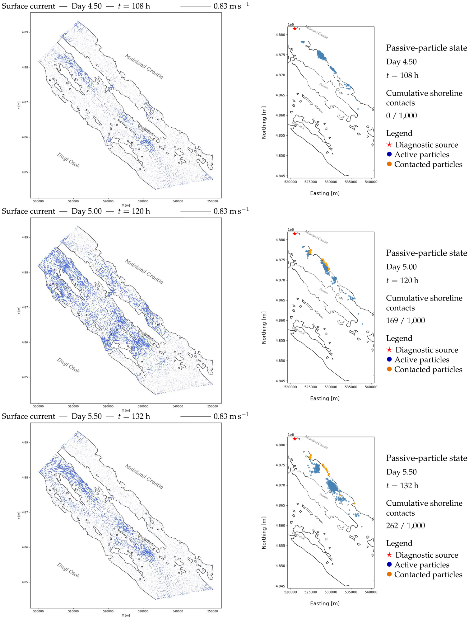
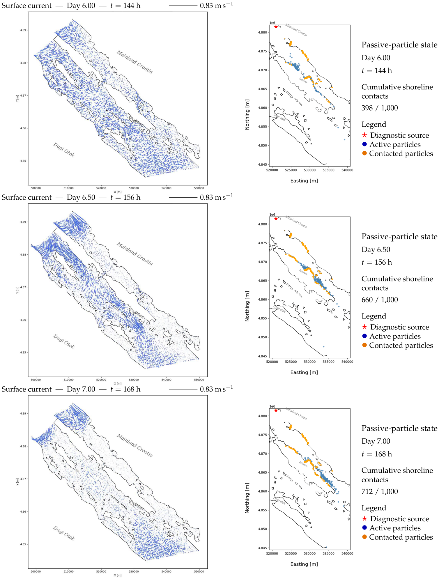
Figure 8 provides the event-period wind context over the Zadar Channel domain. The synchronized current–particle sequence is then shown on three full pages (Figure 9, Figure 10 and Figure 11) using nine matched states from $t=108$ to 192 h (days 4.50–8.00). The cumulative numerical shoreline-contact counts across those nine states are 0, 169, 262, 398, 660, 712, 769, 985, and 1000 particles.

Forcing interpretation and limitation. Figure 8 is a forcing diagnostic, not a validation plot. It shows the first hourly event record, not the storm-maximum field. The $81\times 81$, $0.05°\times 0.05°$ sflux grid is spatially interpolated from ERA5, so its spacing does not add information or resolve local convective gusts below the source-data scale. Arrow lengths are normalized and show direction only; speed is read from the color bar. A complete, quality-controlled set of local wind observations was unavailable for the full interval.

The cumulative-contact series is strongly non-linear. Contact first appears between 108 and 120 h, then rises from 39.8% to 66.0% between 144 and 156 h. A slower interval follows through 180 h, after which the cumulative fraction rises from 76.9% to 98.5% by 186 h and reaches 100% at 192 h. With $t=0$ at 10 June 2025 00:00 UTC, 120 h corresponds to 15 June 00:00 UTC and 156 h to 16 June 12:00 UTC. A substantial part of the cumulative contact therefore predates the documented storm on the evening of 16 June. These changes describe when the evolving current-driven pathway family intersects the model shoreline under the fixed 50 m rule across the full event window; they are neither estimates of a physical deposition rate nor evidence that the storm alone caused the contact sequence.

Because all 1000 particles are released simultaneously and no particles are added later, $G\left(t\right)$ is an empirical cumulative distribution of first numerical shoreline-contact time for one fixed forcing and stochastic realization. The displayed states are 12 h apart from 108 through 180 h and 6 h apart thereafter. The sequence therefore resolves the broad progression of contact, while the exact contact-time distribution remains conditional on the selected output times, random seed, diffusivity, and shoreline rule.

Taken together, Figure 9, Figure 10 and Figure 11 show a staged response rather than an instantaneous collapse of the ensemble onto the shoreline. Cumulative shoreline contact remains zero at 108 h, first appears by 120 h, exceeds one half of the ensemble by 156 h, and all 1000 particles have made numerical shoreline contact by 192 h. The contacted band develops along the channel boundary rather than uniformly across the domain. Under the adopted 50 m hard-contact rule, this is a numerical shoreline-contact diagnostic rather than a physical deposition or permanent-retention model.

4. Discussion

4.1. Resolved Advection, Horizontal Spreading, and Sampled Depth

The sensitivity experiments separate the effects of resolved advection, stochastic horizontal spreading, and sampled depth. Across the three surface-layer cases, a 15-fold change in $K_h$ changes maximum reach from 11.8 to 14.2 km, whereas the corresponding diffusive scale changes from 0.186 to 0.720 km. The resulting reach-to-diffusive-scale ratios of 19.7–63.4 identify resolved channel advection as the dominant control on longitudinal displacement. Horizontal diffusivity remains important because it changes the width of the pathway family and therefore the range of shoreline segments that can be contacted.

The vertical-layer experiment produces the strongest tested response. Sampling L15 rather than L19 reduces 24 h reach by 4.1 km, or 32.8%. This result is consistent with a vertically sheared coastal current and shows why a single depth-independent trajectory cannot represent floating, suspended, and lower-water-column material equally well. In a source–pathway–receptor assessment, the selected velocity layer therefore has a first-order effect on travel time and apparent receptor connectivity.

The current field is calculated by SCHISM from the specified tidal boundary elevations, southern-boundary velocity harmonics, atmospheric forcing, and resolved geometry rather than prescribed from a regional velocity product. During the event period, the imposed southern–northern water-level difference reached approximately 0.07 m. The resulting pressure-gradient response, acceleration through constrictions, and conservation of mass provide a physically coherent process explanation for the along-channel pathways. They do not, however, replace observational validation of the velocity field.

4.2. Meaning of the Virtual-Particle and Shoreline-Contact Results

The 1000-particle ensemble is a numerical sample of possible passive trajectories under one fixed forcing realization, not a representation of 1000 grains, fragments, or units of pollutant mass. The cumulative contact fraction is useful because it records when and where the simulated pathway family first intersects the model shoreline under an explicit 50 m rule. It should not be interpreted as a measured grounding time, deposited mass, or permanent retention probability.

The event sequence therefore answers a limited but clear process question: how does a current-driven passive ensemble encounter the model shoreline when the hydrodynamic field, random seed, diffusivity, release protocol, and contact rule are fixed? Settling, deposition, resuspension, flocculation, particle inertia, direct windage, and Stokes drift are absent. Their inclusion would require material-class parameters and, for wave effects, a locally representative wave solution. The approximately 8 km MFWAM grid is valuable for regional wave context but cannot resolve the sub-kilometre island passages represented by SCHISM. Because a local SCHISM–WWM calculation was not performed, the magnitude of wave–current feedback and Stokes drift remains unknown. The present sequence is consequently a current-driven reference case, not a complete fate model or an estimate of total surface drift.

4.3. Validation Scope and Copernicus Representativeness

The tide-gauge comparison provides an independent observational assessment of the modelled free-surface response that is more appropriate for the present coastal-scale application than comparison with the regional Copernicus current product. The zero-hour optimal lag and high correlation ($r=0.913$) show that SCHISM reproduced the timing and phase of the observed sea-level variations well. The mean bias of 0.012 m indicates close mean alignment over the matched sample under the reference-level convention used for the comparison; it should not be interpreted as a geodetic validation of the vertical datum.

The principal discrepancy was an underestimation of sea-level amplitude. The simulated standard deviation was 0.117 m, or 74.5% of the observed 0.157 m. The tide-gauge record represents total sea-level variability and contains both astronomical-tidal and meteorological contributions, whereas the simulated response depends on the reduced M2–K1 tidal boundary specification, the imposed atmospheric fields, and the representation of regional-scale sea-level variability at the model boundaries. These differences may contribute to the amplitude deficit, but the present comparison does not identify their separate causal effects. Nevertheless, the close phase agreement and zero temporal lag show that the dominant temporal structure of the observed sea-level variations was reproduced during the validation interval.

Agreement in sea level does not constitute direct validation of current velocities within the narrow channel. In the absence of suitable in situ current measurements for the simulation period, direct velocity validation was not possible. The tide-gauge comparison should therefore be interpreted as validation of the modelled sea-level response and its timing rather than as direct observational verification of the local current field.

The all-point Copernicus coverage analysis reinforces this distinction. The narrow interior passages are not represented by valid regional-product sea cells, and the available velocities originate from the southern offshore edge. Their poor agreement with the channel-resolving SCHISM series combines spatial-representativeness error with dynamical differences and cannot isolate SCHISM accuracy. Copernicus is therefore used only to document the absence of a suitable regional validation field inside the passages, not as a substitute for observations.

5. Conclusions

The Zadar Channel simulations identify a clear hierarchy of passive-transport controls under the tested grid, forcing, particle ensemble, and parameterization. Across the 24 h surface-layer tests, a 15-fold change in $K_h$ changes maximum reach from 11.8 to 14.2 km, while sampling the lower L15 velocity field reduces reach from 12.5 to 8.4 km, a 32.8% decrease and the largest tested response. Resolved channel advection controls longitudinal excursion, stochastic diffusion mainly broadens the pathway, and sampled depth has a first-order effect on transport speed and connectivity in this configuration.

Independent hourly observations at the MP Zadar tide gauge provide quantitative validation of the modelled free-surface response. After the first 24 h ramping period, 192 matched pairs give $r=0.913$, a mean bias of 0.012 m, an MAE of 0.051 m, and an RMSE of 0.070 m, with maximum cross-correlation at zero lag. SCHISM reproduces the phase and timing well but underestimates amplitude: the model-to-observation standard-deviation ratio is 0.745. These results support the modelled sea-level response and its timing, but do not directly validate local current vectors.

Under the documented 1000-particle, $K_h=0.5$ m² s⁻¹, $\Delta t_p=450$ s, and 50 m numerical-contact configuration, the June 2025 event-window sequence progresses from zero to full cumulative shoreline contact. Because the release precedes the 16–17 June storm and substantial contact occurs before storm onset, this is a current-driven event-window diagnostic rather than a storm-attribution result or a physical deposition prediction. Copernicus masks the narrow interior passages, and the available offshore velocities agree poorly with SCHISM; the regional product is therefore not used for validation. Suitable HF-radar coverage was also unavailable. Finally, wave–current feedback, Stokes drift, and material-specific fate processes are excluded, so the reported pathways should not be interpreted as total surface drift or pollutant fate.