Multimodal-Augmented Conditional Diffusion Model for Maritime Waypoint-Level Tropical Cyclone Intensity Prediction

Abstract

Accurately forecasting waypoint-level tropical cyclone (TC) intensity, defined as the local wind speed at specific maritime route waypoints under TC influence, is crucial for navigation safety and voyage planning. Conventional studies mainly focus on the central intensity of TC systems and underutilize the complementary value of multimodal meteorological data with inconsistent sampling intervals. To address these challenges, this study proposes a multimodal-augmented conditional diffusion model (MADiff) for waypoint-level TC intensity prediction. To exploit the potential of multimodal inputs, we first design a temporal-adaptive dynamic convolution module (TDConv) to capture multi-timescale features, mitigating multimodal sampling discrepancies without rigid temporal alignment. Second, we develop a discriminative cross-fusion module (DisCF) to aggregate multi-timescale features across diverse modalities, quantifying multimodal heterogeneity and integrating valuable modality-specific features while suppressing noise interference. Fused features are fed into a diffusion model with physics-informed regularization to generate final intensity forecasts. Extensive experiments on four Western North Pacific datasets show that MADiff achieves average MAE and RMSE values of 2.08 kt and 2.37 kt, respectively, for 12 h intensity forecasting. Compared with the state-of-the-art baseline (TC-Clouds-DP), MADiff yields substantial performance improvements, reducing MAE by 16.3% and RMSE by 10.6% on average. This study provides an effective framework for fine-grained TC intensity forecasting, offering valuable insights for extreme marine weather early warning and intelligent navigation decision-making.

1. Introduction

Tropical cyclones (TCs) are extreme systems that produce strong winds, heavy rainfall, and complex mixed sea states characterized by coexisting wind-sea and swell components [1], thereby threatening maritime navigation and transportation safety [2,3,4]. Vessel navigation follows pre-planned routes consisting of discrete waypoints. In this context, the local wind speed induced by TCs (i.e., waypoint-level TC intensity) acts as a critical determinant of local sea state evolution, directly governing navigation safety and operational efficiency. Without accurate forecasts of this intensity, shipping operators are confronted with a dilemma where underestimation risks severe maritime accidents, while overestimation incurs unnecessary costs and delays through excessive route adjustments. Consequently, accurate waypoint-level TC intensity prediction is a prerequisite for optimal navigation decision-making.

TC intensity prediction is inherently a time series forecasting task. Existing research can be classified into dynamical methods [5] and data-driven methods [6,7]. Dynamical methods simulate atmosphere–ocean coupling processes for large-scale forecasts but suffer from coarse spatial resolution and high computational latency. In contrast, data-driven approaches learn evolutionary patterns from historical records via statistical or deep learning architectures, with fast inference and strong generalization [8], and have thus attracted extensive attention. However, existing data-driven methods still have two critical limitations when applied to waypoint-level maritime scenarios.

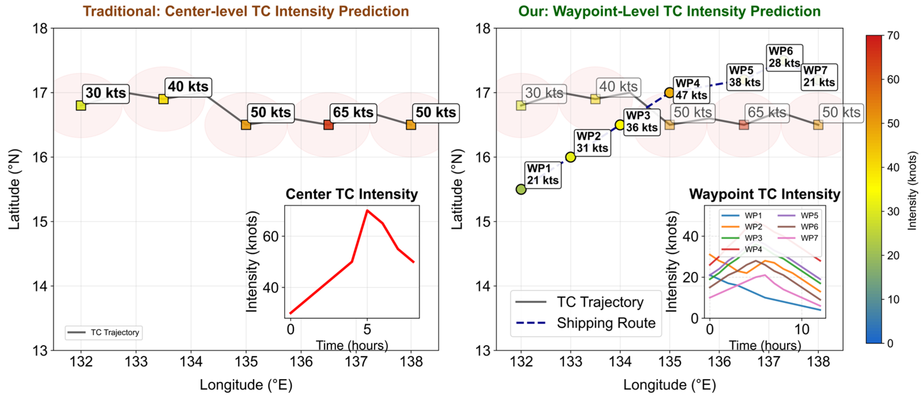
On the one hand, existing studies primarily focus on center-level TC intensity prediction (i.e., the central intensity of the cyclone). In real-world maritime scenarios, center-level TC intensity forecasts provide only limited guidance for navigation decision-making and cannot precisely reflect the actual risks at individual waypoints. Figure 1 illustrates the differences between center-level and waypoint-level TC intensity forecasts. The pink circular area represents the influence range of a tropical cyclone, with the cyclone center at its geometric center. WP denotes a fixed maritime waypoint along shipping routes, which remains independent of the TC movement track.

On the other hand, TC intensity evolution is a dynamically coupled process governed by atmospheric, oceanic, and geographic factors, exhibiting strong nonlinearity and inherent uncertainty. Most existing methods rely heavily on unimodal data (e.g., satellite imagery), posing significant challenges in capturing such complex dynamics. Although a few studies have attempted to incorporate multimodal data, they often struggle to align the distinct sampling intervals and inherent heterogeneity of these diverse inputs. More critically, these methods follow a deterministic prediction paradigm [9,10] that outputs only a single, fixed intensity value without probabilistic uncertainty quantification, reducing robustness in complex and variable marine environments.

To address these challenges, this study proposes a multimodal-augmented conditional diffusion model (MADiff) for waypoint-level TC intensity prediction. By combining the complementary properties of multimodal data and the powerful probabilistic modeling capability of diffusion models, the proposed MADiff is naturally well-suited for waypoint-level TC intensity prediction. The main contributions of this study are summarized as follows:

(1) A multimodal-augmented conditional diffusion model (MADiff) is proposed for waypoint-level TC intensity prediction, tailored to fine-grained maritime navigation safety demands.

(2) A temporal-adaptive dynamic convolution module (TDConv) is designed, which adaptively adjusts kernel sizes within predefined physical temporal windows and generates convolutional parameters via timestamp embeddings, thus mitigating multimodal sampling discrepancies and yielding consistent multi-timescale features without requiring rigid temporal alignment.

(3) A discriminative cross-fusion module (DisCF) is developed, which quantifies cross-modal heterogeneity via information entropy and adopts sparse attention with discriminative selection to integrate valuable complementary features while filtering out redundant interference, thus generating robust and comprehensive multimodal representations.

(4) Extensive experiments demonstrate the superior performance and remarkable cross-basin generalization of MADiff for waypoint-level TC intensity prediction.

The remainder of this article is organized as follows. Section 2 reviews related work on TC intensity prediction and diffusion models. Section 3 introduces the multimodal meteorological data and formulates the waypoint-level TC intensity prediction problem. Section 4 elaborates on the proposed MADiff model in detail. Section 5 presents the experimental results and their analysis. Finally, Section 6 summarizes this work and discusses the limitations along with potential directions for future work.

2. Related Work

2.1. TC Intensity Prediction

TC intensity prediction is a significant challenge in oceanic meteorology. Against the backdrop of meteorological big data, the development of data-driven approaches for TC intensity prediction has emerged as a prominent research focus. These methods can be roughly divided into statistical methods and deep learning methods.

Statistical Methods. In the early stages, constrained by the insufficient quantity and limited diversity of meteorological data as well as the limitations of forecasting techniques, researchers manually design and extract predictive features from historical meteorological records and adopt statistical models for TC intensity prediction. Neumann et al. [11] proposed the Climatology and Persistence (CLIPER) model, which integrates climate patterns and the persistence of features observed during the early phases of TC development. DeMaria et al. [12] developed the Statistical Hurricane Intensity Prediction Scheme (SHIPS), incorporating sea surface temperature, vertical wind shear, and persistence as key predictive factors. Chavas et al. [13] introduced an efficient linear empirical model that incorporates maximum wind speed, wind radius, TC center latitude, and ambient pressure as input parameters. However, such methods fail to characterize complex and nonlinear atmospheric variations, particularly when faced with unseen events like extreme TCs or substantial climate change impacts. This inherent limitation leads to degraded predictive accuracy and reliability, ultimately restricting the practical effectiveness of these statistical methods.

Deep Learning Methods. With the massive and continuous accumulation of meteorological data and the remarkable breakthroughs in deep learning, developing diverse deep learning models for TC intensity prediction has become a promising approach. Early studies mainly relied on unimodal data, with satellite imagery serving as the most prevalent modality for TC analysis. Alijoyo et al. [14] proposed a hybrid architecture based on CNN and Bi-LSTM, which can effectively capture the complex TC evolution patterns from infrared satellite imagery. Wang et al. [15] combined convolutional neural networks with low-rank tensor analysis techniques to process multispectral satellite imagery and proposed an integrated framework for TC data augmentation and analysis. Wu et al. [16] introduced a multi-task machine learning framework based on satellite imagery, which is capable of predicting both the track and intensity of TCs simultaneously. However, unimodal data is inadequate to fully depict the entire TC evolution process, especially when the input data is incomplete or unavailable. Therefore, researchers have attempted to incorporate multimodal data [17]. Wang et al. [18] proposed a multi-modal multi-scale causal autoregressive model (MSCAR), which integrates satellite imagery and numerical data for global TC intensity autoregressive forecasting. Li et al. [19] introduced a multimodal adversarial fusion approach, which fuses TC observational data and ERA-Interim reanalysis data by using adversarial learning to eliminate the modal gap, thereby improving the accuracy of TC intensity forecasting. In addition, many classic general-purpose [20] and application-oriented [21] time-series forecasting models can be applied to TC intensity prediction, and they often outperform traditional statistical and shallow machine learning models. However, these methods cannot effectively handle the distinct sampling intervals and inherent heterogeneity of multimodal meteorological inputs, and fail to model the probabilistic distribution of prediction outputs. More critically, they only focus on the central intensity and overall structural characteristics of TCs, thereby being unable to provide fine-grained intensity forecasts for specific maritime waypoints. This limitation severely restricts their practical applicability in real-world maritime transportation scenarios.

2.2. Diffusion Models

Diffusion models are a powerful generative framework, comprising a diffusion process and a reverse process. The former gradually adds noise to real data, while the latter removes the introduced noise to generate realistic data [22]. Moreover, diffusion models can generate samples that meet specific requirements through the integration of conditional information. The authenticity and diversity of these generated samples are far superior to those of conventional deep learning models [23,24,25]. Zhu et al. [26] proposed a conditional text-image generation method, which can generate realistic and diverse 2D image samples under given image, text, and style conditions. Höllein et al. [27] proposed a 3D image generation diffusion model by incorporating pre-trained text-image models as prior knowledge. Hao et al. [28] proposed a motion-aware text-to-video (T2V) diffusion model that generates high-quality, fluid videos guided by text prompts.

Additionally, several studies have applied diffusion models to time series completion [29,30] and prediction [31]. For example, Shen et al. [32] proposed a novel multimodal view framework that takes time series images as conditional information and leverages diffusion models for long-term time series prediction. The unique advantages of diffusion models render them well-suited for characterizing multimodal data distributions, thereby offering a promising solution for mitigating the inherent limitations of current TC intensity prediction methods. However, TC intensity prediction faces unique challenges, including multimodal sampling discrepancies, inherent cross-modal heterogeneity, and physical constraints governing TC evolutionary processes. Unfortunately, existing diffusion-based time series models struggle to achieve reliable performance in this meteorological-specific task. To tackle these practical issues, this study proposes a multimodal-augmented conditional diffusion model (MADiff) for waypoint-level TC intensity prediction. MADiff takes multimodal meteorological data as conditional inputs and integrates customized TDConv for multi-timescale feature extraction, DisCF for heterogeneous cross-modal fusion, and physics-informed regularization. These dedicated designs enable MADiff to capture waypoint-level TC intensity distribution more precisely and comprehensively, with improved physical rationality and stronger adaptability to complex multimodal meteorological data.

3. Problem Definition

3.1. Multimodal Meteorological Data and Their Timestamps

This study focuses on waypoint-level TC intensity prediction, and emphasizes the use of multimodal data, including numerical meteorological data, infrared satellite imagery, and TC-related texts. Next, we describe these data in detail.

(1) Numerical meteorological data are used to precisely characterize the meteorological changes at maritime waypoints. For a maritime waypoint, the meteorological numerical data at time $t$ can be denoted as $X_N^t\in {\mathbb{R}}^{C_N}$, where $C_N$ represents the number of meteorological elements. Based on the TC generation mechanism, this study focuses on three elements: sustained wind speed (quantitative indicator of TC intensity), temperature, and air pressure, so $C_N=3$. These data are obtained from the ERA5 dataset [33] according to the latitude and longitude of the target waypoints. The ERA5 dataset, released by the European Centre for Medium-Range Weather Forecasts, has a spatial resolution of ${0.25}^{\circ }\times {0.25}^{\circ }$ and a time sampling interval of 1 h.

(2) Infrared satellite imagery is utilized to visually present the cloud distribution over the local sea area of a maritime waypoint. For a maritime waypoint, the infrared satellite imagery at time $t$ can be denoted as $X_I^t\in {\mathbb{R}}^{H\times W}$, where $H$ and $W$ represent the height and width of the image, respectively. Raw infrared satellite imagery covers a broad area and contains a large amount of redundant information irrelevant to the target waypoints. To address this, this study crops the original infrared satellite imagery to obtain a local satellite image (256 $\times$ 256 pixels, corresponding to 20 latitude units multiplied by 20 longitude units) centered on the target waypoints. The original infrared satellite imagery used in this study is from the GridSat-B1 dataset [34], with a spatial resolution of ${0.07}^{\circ }\times {0.07}^{\circ }$ and a time sampling interval of 3 h.

(3) TC-related texts are used to represent TC conditions and their spatial relationships with maritime waypoints. These texts are composed of two natural components without any artificial construction. The first component is the TC state information, which is directly extracted from the CMA Best Track Dataset (CMA_BT) released by the China Meteorological Administration [35,36], including the TC center location, maximum sustained wind speed and minimum central pressure. The second component is the relative positional relationship between the TC center and the target waypoint, which is calculated in real time from the TC center coordinates (from CMA_BT) and the fixed waypoint coordinates. All data are sampled at a 6 h temporal interval. A typical example is as follows: TC Aiyunni is located at 23.1 °N, 112.3 °E, with a maximum sustained wind of 18 m/s and a minimum central pressure of 996 hPa. The TC center is 50 km away from the target waypoint. For a maritime waypoint, the TC-related texts at time $t$ can be denoted as $X_T^t\in {\mathsf{\Omega }}^{C_T}$, where $\mathsf{\Omega }$ represents the set of words and $C_T$ denotes the text length.

The aforementioned multimodal data simultaneously encode both the global features of TC systems and the specific attributes of individual maritime waypoints, thereby enabling accurate prediction of waypoint-level TC intensity. These multimodal meteorological data present inconsistent temporal sampling intervals. Therefore, beyond the aforementioned data, this study further incorporates timestamps as auxiliary features. For each timestamp, we extract the season, month, day, hour, minute, and second to form a feature vector. For example, for the timestamp 2020-10-25 08:30:00 at time $t$, its feature vector is $S^t=\left(3, 10, 25, 08, 30, 00\right)\in {\mathbb{R}}^6$.

3.2. Problem Definition of Waypoint-Level TC Intensity Prediction

For a maritime waypoint, given the historical multimodal meteorological data over the past $p$ time steps, including numerical meteorological data $X_N=\left\{X_N^{t-p}, X_N^{t-p+1}, \dots , X_N^t\right\}\in {\mathbb{R}}^{l_N\times 3}$ and its timestamps $S_N=\left\{S_N^{t-p}, S_N^{t-p+1}, \dots , S_N^t\right\}\in {\mathbb{R}}^{l_N\times 6}$, infrared satellite imagery $X_I=\left\{X_I^{t-p}, X_I^{t-p+3}, \dots ,{ X}_I^t\right\}\in {\mathbb{R}}^{l_I\times H\times W}$ and its timestamps $S_I=\left\{S_I^{t-p},{ S}_I^{t-p+3}, \dots , S_I^t\right\}\in {\mathbb{R}}^{l_I\times 6}$, TC-related texts $X_T=\left\{X_T^{t-p}, X_T^{t-p+6}, \dots , X_T^t\right\}\in {\mathsf{\Omega }}^{l_T\times C_T}$ and its timestamps $S_T=\left\{S_T^{t-p}, S_T^{t-p+6}, \dots ,{ S}_T^t\right\}\in {\mathbb{R}}^{l_T\times 6}$, where $l_N=p+1$, $l_I={\displaystyle \frac{p}{3}}+1$, $l_T={\displaystyle \frac{p}{6}}+1$ represent the number of records for numerical, imagery, and text data, respectively. Our objective is to predict the waypoint-level TC intensity (i.e., the local wind speed at this waypoint under TC influence). The problem is defined as:

$$Y^{t+n}=f\left(X_N,{ S}_N,{ X}_I, S_I, X_T, S_T\right)$$

(1)

where $Y^{t+n}$ represents the predicted waypoint-level TC intensity at time $t+n$ and $n$ denotes the time interval between the current time and the future time, and $f$ is our predictive model trained on historical multimodal meteorological data. To better utilize multimodal data, $p$ is set as a common multiple of the time intervals of the multimodal data, for instance, 12, 24, and so on.

For clarity, the notations and corresponding descriptions are listed in

Table 1. Summary of frequently used notations.

Notation	Description
$X_N,X_I,X_T$	The multimodal data, numerical meteorological data ($X_N$), infrared satellite imagery ($X_I$), TC-related texts ($X_T$)
$X_N^t,X_I^t, X_T^t$	The multimodal data at time t
$S_N, S_I,S_T$	The timestamps of multimodal data
$S_N^t, S_I^t, S_T^t$	The feature vectors of timestamps at time t
$l_N, l_I, l_T$	The number of records of multimodal data
$Y^{t+n}$	The TC intensity at time $t+n$
$Y_k^{t+n}$	The output of the k-th diffusion step, $Y_0^{t+n}=Y^{t+n}$
$k, K$	The diffusion step and its maximum value
${\beta }_k$	The variance of Gaussian noise during the k-th diffusion step
$z_k, {\tilde{z}}_k$	The Gaussian noise during the k-th diffusion step and its prediction
$d$	The feature dimension
$D^t$	The distance between the waypoint and TC center at time t
${\tilde{Y}}_{max}^t$	The maximum sustained wind speed of TC center at time t
$D_{max}^{t+n}$	The radius of maximum sustained wind of TC at time t
$Z_N,Z_I,Z_T$	The preprocessing representations of multimodal data
$Z_{N,m}, Z_{I,m}, Z_{T,m}$	The multimodal features extracted at the m-th timescale
$F_m$	The multimodal fusion vector of the m-th timescale
$F_{MC}$	The final multimodal fusion result
$g, G$	The number of generations and its maximum value

.

4. Multimodal-Augmented Conditional Diffusion Model

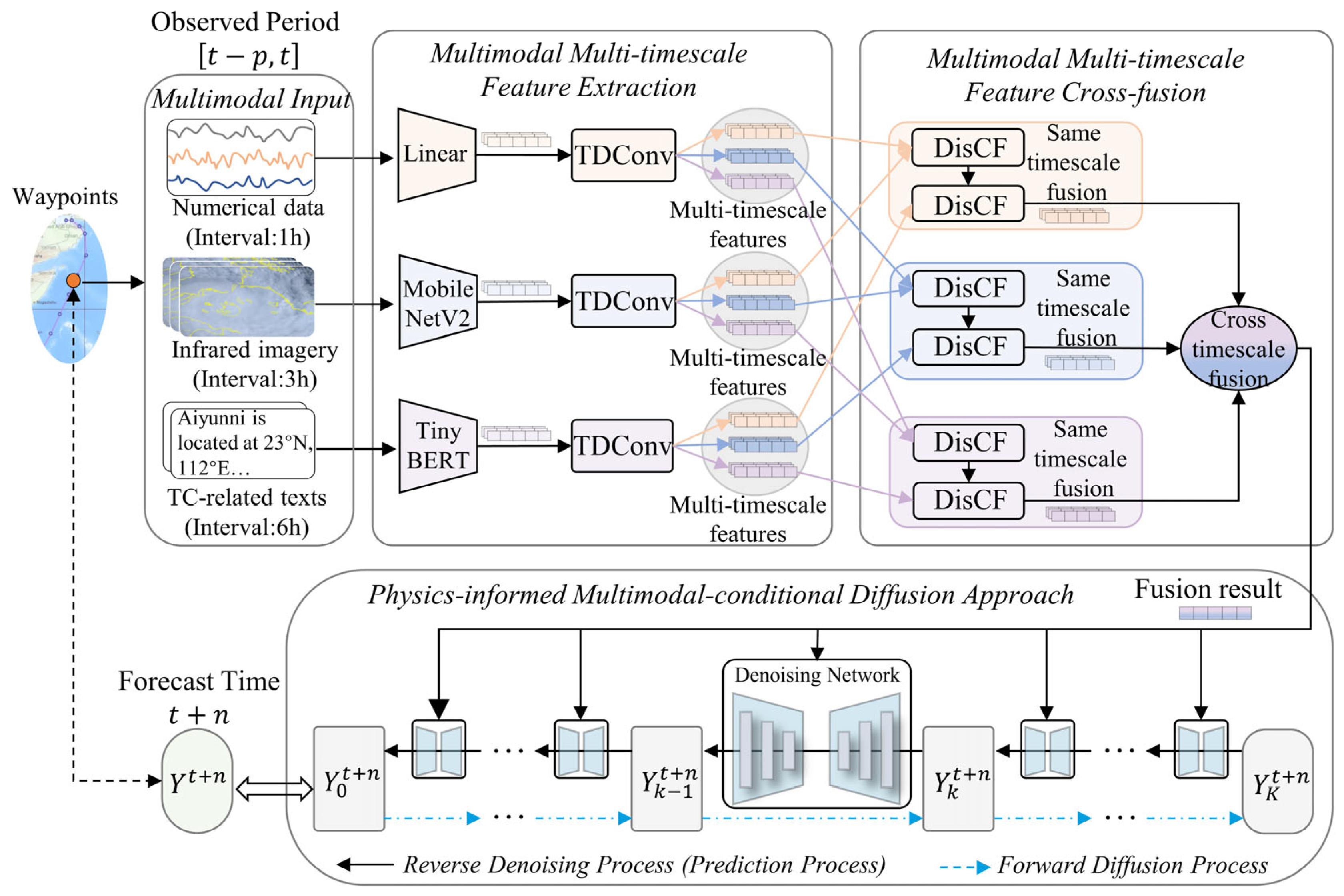
In this section, we propose a multimodal-augmented conditional diffusion model (MADiff) for waypoint-level TC intensity prediction. Figure 2 illustrates the overall framework of the proposed MADiff. First, we elaborate on the process of leveraging the diffusion model, which serves as the backbone of our framework, to predict waypoint-level TC intensity. Subsequently, we introduce the multi-timescale feature extraction and fusion processes for multimodal data, both of which are critical for enhancing the accuracy of TC intensity prediction.

4.1. Physics-Informed Multimodal-Conditional Diffusion Approach

Waypoint-level TC intensity prediction involves inevitable predictive uncertainty. As a typical generative paradigm, diffusion models can effectively characterize this inherent stochasticity. However, as a purely data-driven approach, standard diffusion models tend to generate physically unreasonable intensity trajectories, especially for long-horizon forecasting tasks. To this end, this study proposes a physics-informed multimodal-conditional diffusion approach for waypoint-level TC intensity prediction. This approach adopts multimodal meteorological data as conditional guidance and introduces a physics-informed dynamics loss to regularize the diffusion process, thereby ensuring that predicted results conform to the fundamental laws of atmospheric dynamics.

Our approach consists of a forward diffusion process and a reverse denoising process. Specifically, in the forward diffusion process, Gaussian noise is gradually added K times to transform the original TC intensity $Y_0^{t+n}=Y^{t+n}$ into $Y_K^{t+n}$. This process is defined as follows:

$$\begin{gathered} q\left(Y_{1:K}^{t+n}|Y_0^{t+n}\right)={\displaystyle \prod _{k=1}^K}q\left(Y_k^{t+n}|Y_{k-1}^{t+n}\right) \\ q\left(Y_k^{t+n}|Y_{k-1}^{t+n}\right)=\mathcal{N}\left(Y_k^{t+n}; \sqrt{1-{\beta }_k}{Y}_{k-1}^{t+n}, {\beta }_k\mathbf{I}\right) \end{gathered}$$

(2)

where $k\in \left\{1, 2, 3, ..., K\right\}$ represents the diffusion step, ${\beta }_k\in \left(0, 1\right)$ denotes the incremental hyperparameter that controls the variance of added noise. When K is sufficiently large, $Y_K^{t+n}$ approximates Gaussian noise. To enhance the efficiency of the diffusion process, we employ the reparameterization technique [22] to modify Equation (2) into $q\left(Y_k^{t+n}|Y_0^{t+n}\right)=\mathcal{N}\left(Y_k^{t+n}; \sqrt{{\overline{\alpha }}_k}{Y}_0^{t+n},\left(1-{\overline{\alpha }}_k\right)\mathbf{I}\right)$. Then, we directly sample $Y_k^{t+n}$ as $Y_k^{t+n}=\sqrt{{\overline{\alpha }}_k}{Y}_0^{t+n}+\sqrt{1-{\overline{\alpha }}_k}{z}_k$, where ${\alpha }_k=1-{\beta }_k$, ${\overline{\alpha }}_k={\prod }_{i=1}^k{\alpha }_i$, and $z_k\in \mathcal{N}\left(0,\mathbf{I}\right)$ is the Gaussian noise.

The inverse process is conditioned on multimodal meteorological data. Its goal is to recover the original TC intensity $Y_0^{t+n}$ from the Gaussian noise $Y_K^{t+n}$ by accurately predicting and removing the noise introduced during the diffusion process. This process is defined as follows:

$$\begin{gathered} p_{\theta }\left(Y_{1:K}^{t+n}|F_{MC}\right)=p\left(Y_K^{t+n}\right){\displaystyle \prod _{k=1}^K}{p}_{\theta }\left(Y_{k-1}^{t+n}|Y_k^{t+n}, F_{MC}\right) \\ {p}_{\theta }\left(Y_{k-1}^{t+n}|Y_k^{t+n}, F_{MC}\right)=\mathcal{N}\left(Y_{k-1}^{t+n}; {\mu }_{\theta }\left(Y_k^{t+n}, k, F_{MC}\right), {\sigma }_k^2\mathbf{I}\right) \end{gathered}$$

(3)

where $F_{MC}=\mathrm{F}\mathrm{usion}\left(X_N, X_I, X_T, S_N,{ S}_I, S_T\right)$ represents the conditional information, i.e., the multimodal fusion vector, $\mathrm{Fusion}\left(·\right)$ denotes the multimodal fusion function. ${\mu }_{\theta }$ and ${\sigma }_k^2$ represent the mean and variance of the conditional distribution $p_{\theta }\left(Y_{k-1}^{t+n}|Y_k^{t+n}, F_{MC}\right)$, respectively. In this work, ${\sigma }_k^2={\displaystyle \frac{1-{\overline{\alpha }}_{k-1}}{1-{\overline{\alpha }}_k}}{\beta }_k$, and the parameterization of ${\mu }_{\theta }$ can be defined as follows:

$${\mu }_{\theta }\left(Y_k^{t+n}, k,{ F}_{MC}\right)={\displaystyle \frac{1}{\sqrt{{\alpha }_k}}}\left(Y_k^{t+n}-{\displaystyle \frac{{\beta }_k}{\sqrt{1-{\overline{\alpha }}_k}}}{z}_{\theta }\left(Y_k^{t+n}, k, F_{MC}\right)\right)$$

(4)

where $z_{\theta }$ is the denoising network, which takes the noisy sample $Y_k^{t+n}$, denoising step k, and condition $F_{MC}$ as inputs to estimate the noise $z_k$ added during the diffusion process and gradually recovers the original TC intensity.

During training, the diffusion model typically relies on the noise prediction loss, which guides the denoising network to predict the injected Gaussian noise and perform gradual denoising to generate waypoint-level TC intensity:

$${\mathcal{L}}_{diff}={\mathbb{E}}_{Y_0^{t+n}, z_k}\left[{\Vert z_k-z_{\theta }\left(Y_k^{t+n}, k, F_{MC}\right)\Vert }_2^2\right]$$

(5)

To enforce physical consistency in predictions, we introduce a physics-informed dynamics loss that embeds essential atmospheric dynamic principles, guiding predictions to conform to fundamental laws of atmospheric motion:

$${\mathcal{L}}_{phy}={\mathbb{E}}_{t, n}\left[{\Vert {\displaystyle \frac{d{Y}^{t+n}}{dt}}-{\displaystyle \frac{d{\tilde{Y}}^{t+n}}{dt}}\Vert }_2^2\right]$$

(6)

where ${\displaystyle \frac{d{Y}^{t+n}}{dt}}$ and ${\displaystyle \frac{d{\tilde{Y}}^{t+n}}{dt}}$ are the temporal derivatives of the predicted TC intensity and theoretical TC intensity, respectively. In practice, the temporal derivatives are approximated using first-order finite differences between consecutive time steps, to adapt to the discrete characteristics of TC intensity prediction. The theoretical TC intensity ${\tilde{Y}}^{t+n}$ is derived from the Jelesnianski hurricane model [37,38] and is formulated as:

$${\tilde{Y}}^{t+n}=\left\{\begin{array}{cc}\hfill {\tilde{Y}}_{max}^{t+n},& D^{t+n}\le D_{max}^{t+n}\hfill \\ {\tilde{Y}}_{max}^{t+n}\times {\left({\displaystyle \frac{D_{max}^{t+n}}{D^{t+n}}}\right)}^{\delta },& D^{t+n}>D_{max}^{t+n}\hfill \end{array}\right.$$

(7)

where $D^{t+n}$ is the distance between the target waypoint and TC center, $D_{max}^{t+n}$ is the radius of maximum wind, ${\tilde{Y}}_{max}^{t+n}$ is the maximum sustained wind speed, and $\delta \in \left[1.0, 2.0\right]$ is the radial decay index. Notably, all TC structural parameters used to calculate the theoretical intensity ${\tilde{Y}}^{t+n}$ at the target time $t+n$ are sourced from official operational forecasts (China Meteorological Administration). These forecast products are publicly available at the forecast initialization moment in real operational scenarios, which ensures the information boundary is completely consistent between model training and inference, and no post-event observation data that is unavailable at initialization is introduced.

Finally, we integrate the two losses into the total objective function:

$${\mathcal{L}}_{total}={\mathcal{L}}_{diff}+{\lambda \mathcal{L}}_{phy}$$

(8)

where $\lambda$ is a hyperparameter for balancing the noise prediction loss and physics-informed dynamics loss. This total loss preserves the probabilistic generative capability of the diffusion model while explicitly imposing atmospheric dynamics constraints, enhancing the robustness of long-horizon TC intensity forecasts.

With the above framework, waypoint-level TC intensity prediction can be effectively implemented. However, fully exploiting and fusing multimodal meteorological data remains critical for further improving prediction accuracy. To this end, this study develops a dedicated multimodal fusion method, which is elaborated in the subsequent sections.

4.2. Multimodal Multi-Timescale Feature Extraction

Across different timescales, TC intensity variations exhibit distinct patterns, such as short-term fluctuations and long-term evolutionary trends. However, capturing these multi-timescale patterns from multimodal meteorological data remains challenging due to inherent cross-modal heterogeneity in feature representations, dimensional discrepancies, and inconsistent sampling intervals across modalities. To address these issues, this section first unifies heterogeneous multimodal data into consistent embeddings and further proposes a temporal-adaptive dynamic convolution (TDConv) to extract multi-timescale features under interval-inconsistent sampling conditions. This design enables the extracted multi-timescale features to maintain consistent temporal semantics and alleviate sampling-induced misalignment, laying a solid foundation for subsequent multimodal feature fusion.

4.2.1. Multimodal Embedding and Dimension Unification

To prepare unified inputs for multi-timescale feature learning, this study extracts unified-dimensional embeddings for each modality from meteorological numerical data, infrared satellite imagery, and TC-related texts via modality-specific encoders.

First, we map numerical meteorological data $X_N\in {\mathbb{R}}^{l_N\times 3}$ into $Z_N\in {\mathbb{R}}^{l_N\times d}$ via linear projection, formalized as $Z_N=W^N\left(W^L{X}_N\right)\in {\mathbb{R}}^{l_N\times d}$, where $W^L$ denotes the linear projection matrix, $W^N$ represents the alignment parameters for multimodal dimension unification, and $d$ is the unified embedding dimension.

Second, we employ a pre-trained MobileNetV2 [39] to encode infrared satellite imagery $X_I\in {\mathbb{R}}^{l_I\times H\times W}$ into $Z_I\in {\mathbb{R}}^{l_I\times d}$, formalized as $Z_I=W^I\left(\mathrm{Flatten}\left(\mathrm{MobileNetV}2\left(X_I\right)\right)\right)$, where $\mathrm{Flatten}\left(\cdot \right)$ denotes the operation of flattening the convolutional feature map into a 1D vector, and $W^I$ also represents alignment parameters.

Finally, we employ a pre-trained TinyBERT [40] to obtain the feature representation $Z_T\in {\mathbb{R}}^{l_T\times d}$ of TC-related texts $X_T\in {\mathsf{\Omega }}^{l_T\times C_T}$, formalized as $Z_T=W^T\left(\mathrm{T}\mathrm{i}\mathrm{n}\mathrm{y}\mathrm{B}\mathrm{E}\mathrm{R}\mathrm{T}\left(X_T\right)\right)$, where $W^T$ also acts as alignment parameters.

4.2.2. Multi-Timescale Feature Extraction

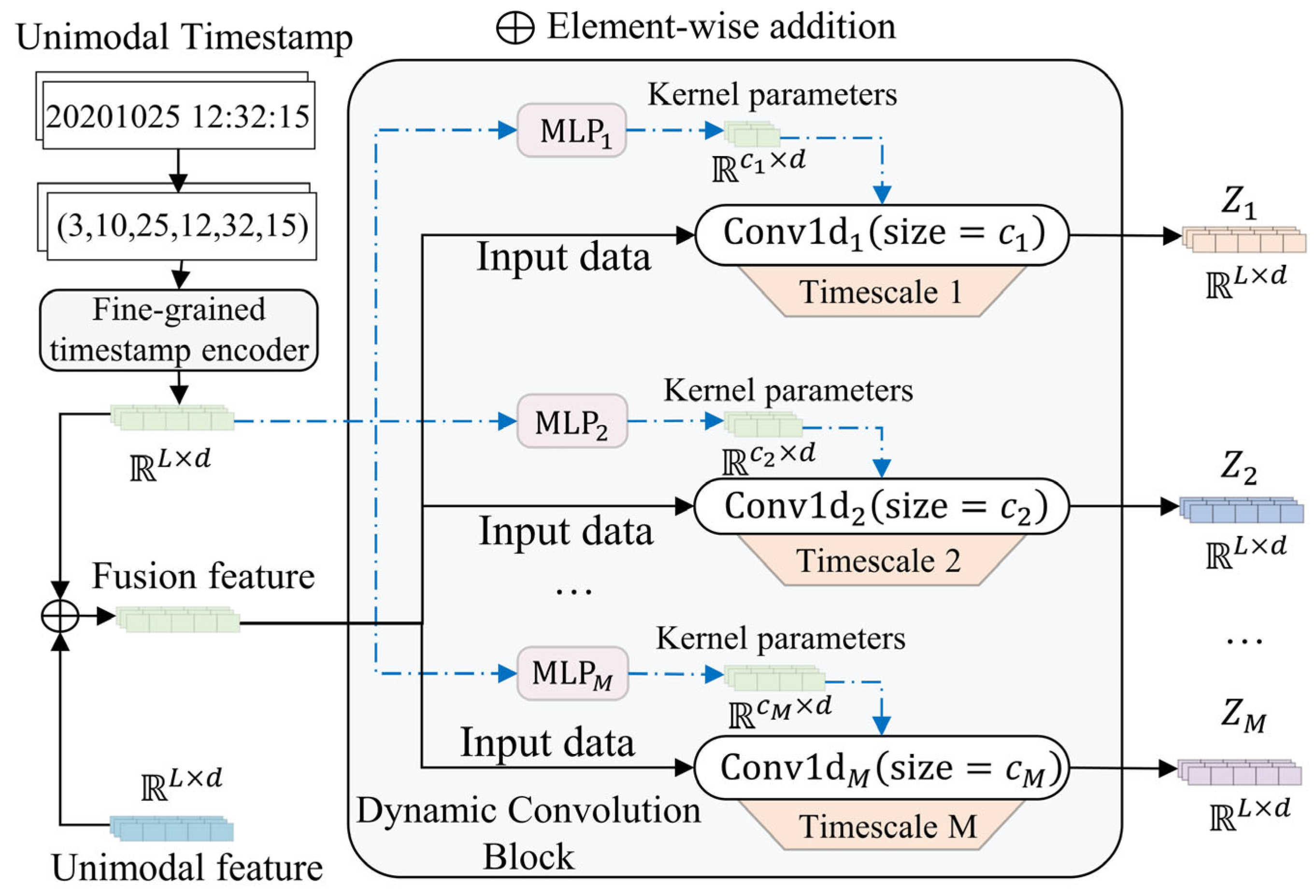
Multimodal meteorological data naturally presents interval-inconsistent sampling characteristics (e.g., hourly numerical data, 3-hourly satellite imagery). Extracting multi-timescale features via 1D convolutions with different kernel sizes is a classic approach, yet such methods require strictly synchronized time series. Forced multimodal temporal alignment via trimming or interpolation inevitably impairs data fidelity and induces redundant noise. In contrast, direct modeling without alignment leads to cross-modal temporal semantic misalignment. These issues significantly degrade multimodal fusion performance. To address these challenges, this study proposes a temporal-adaptive dynamic convolution module (TDConv), which leverages fine-grained temporal information from timestamps to dynamically generate convolutional parameters, simultaneously realizing interval inconsistency adaptation and multi-timescale feature extraction without mandatory temporal alignment. The overall architecture of TDConv is illustrated in Figure 3, which mainly consists of a fine-grained timestamp encoder and a dynamic convolution block.

Given a unimodal feature sequence $Z=\left\{z^1, z^2, \dots , z^L\right\}\in {\mathbb{R}}^{L\times d}$ and its corresponding timestamps $S=\left\{S^1, S^2, \dots ,{ S}^L\right\}\in {\mathbb{R}}^{L\times 6}$. To fully exploit the temporal information contained in timestamps, TDConv first generates a continuous embedding for each timestamp via the fine-grained timestamp encoder, which leverages sine and cosine functions based on meteorological periodicity priors of each temporal feature (e.g., a 12-month period for monthly features, and a 24 h period for hourly features). For a timestamp $S^l\in S$, its embedding $h^l$ can be calculated as follows:

$$h^l=\mathrm{Concat}\left(h^{l,1}, h^{l,2},\dots ,{ h}^{l,6}\right)W^S$$

(9)

where $h^l\in {\mathbb{R}}^d$, $\mathrm{Concat}\left(\cdot \right)$ denotes vector concatenation, and $W^S\in {\mathbb{R}}^{6d\times d}$ represents the linear transformation parameters. $h^{l,i}\in {\mathbb{R}}^d$ denotes the embedding of the i-th temporal feature $S^{l,i}$ of timestamp $S^l$, which can be computed as follows:

$$\left\{\begin{array}{c}{h}_{2j}^{l,i}=\sin \left(2\pi S^{l,i}/{\left({\tau }_i\right)}^{{\displaystyle \frac{2j}{d}}}\right)\\ h_{2j+1}^{l,i}=\cos \left(2\pi S^{l,i}/{\left({\tau }_i\right)}^{{\displaystyle \frac{2j}{d}}}\right)\end{array}\right.$$

(10)

where $h_{2j}^{l,i}$ and $h_{2j+1}^{l,i}$ denote the even and odd dimensions of $h^{l,i}$, respectively, and ${\tau }_i$ represents the periodic value of the i-th temporal feature. As a result, this study denotes the embeddings of all timestamps as $H=\left\{h^1, h^2, \dots ,{ h}^L\right\}\in {\mathbb{R}}^{L\times d}$.

Then, the unimodal feature sequence and its timestamp embeddings are fed into the dynamic convolution block to extract multi-timescale features. Different from traditional convolutions that define timescales based on fixed sampling points and adopt globally invariant kernel parameters, TDConv defines each timescale with a fixed physical temporal window (e.g., 6 h, 12 h). It generates adaptive kernel weights from the timestamp embedding at each time step. This design allows convolution kernels to perceive temporal intervals, sampling rates and periodic features in real time, automatically filter valid samples in the predefined physical window based on absolute timestamps, and adapt to multimodal meteorological data with distinct sampling intervals. For the m-th 1D convolution (${\mathrm{C}\mathrm{o}\mathrm{n}\mathrm{v}1\mathrm{D}}_m$) with kernel size $c_m$, the parameters ${\mathrm{W}}_m^l$ at time $l$ are dynamically generated via a scale-specific multilayer perceptron (MLP). The generation process can be defined as follows:

$${\mathrm{W}}_m^l=\mathrm{R}\mathrm{e}\mathrm{s}\mathrm{h}\mathrm{a}\mathrm{p}\mathrm{e}\left({\mathrm{M}\mathrm{L}\mathrm{P}}_m\left(h^l\right)\right)$$

(11)

where ${\mathrm{W}}_m^l\in {\mathbb{R}}^{c_m\times d}$, ${\mathrm{MLP}}_m(·)$ is the function of the m-th MLP, and $\mathrm{Reshape}(·)$ transforms the flattened output of ${\mathrm{M}\mathrm{L}\mathrm{P}}_m\left(h^l\right)$ (a vector of length $c_m\times d$) into the $c_m\times d$ kernel matrix.

With dynamically generated kernels, the output of ${\mathrm{C}\mathrm{o}\mathrm{n}\mathrm{v}1\mathrm{D}}_m$ can be further obtained and denoted as $Z_m=\left\{z_m^1, z_m^2, \dots , z_m^L\right\}\in {\mathbb{R}}^{L\times d}$, where $z_m^l$ represents the output at time l and can be computed as follows:

$$z_m^l=\mathrm{R}\mathrm{e}\mathrm{L}\mathrm{U}\left(\mathrm{s}\mathrm{u}\mathrm{m}\left({\tilde{Z}}^{\left[l-{\alpha }_m, l+{\alpha }_m\right]}\odot {\mathrm{W}}_m^l\right)\right)$$

(12)

where $\tilde{Z}=Z+H$ denotes the fused features of unimodal features and timestamp embeddings; ${\tilde{Z}}^{\left[l-{\alpha }_m, l+{\alpha }_m\right]}\in {\mathbb{R}}^{c_m\times d}$ denotes the fused features within the physical temporal window $\left[l-{\alpha }_m, l+{\alpha }_m\right]$, ${\alpha }_m={\displaystyle \frac{c_m-1}{2}}$; $\odot$ represents the Hadamard product, $\mathrm{sum}(·)$ is the summation operation performed along the time dimension of the temporal window for each feature channel independently.

After traversing all scales, M groups of 1D convolution outputs are obtained, forming the final multi-timescale feature set $\left\{Z_1, Z_2, \dots , Z_M\right\}$. These features capture short-term fluctuations, medium-term trends and long-term evolutionary patterns of TC intensity, providing comprehensive temporal information for subsequent multimodal fusion.

Based on the designed TDConv module, multi-timescale features can be extracted independently for each data modality: meteorological numerical data $\left\{Z_{N,1}, Z_{N,2}, \dots , Z_{N,M}\right\}=\mathrm{TDConv}\left(Z_N, S_N\right)$, infrared satellite imagery $\left\{Z_{I,1}, Z_{I,2}, \dots ,Z_{I,M}\right\}=\mathrm{TDConv}\left(Z_I, S_I\right)$, and TC-related texts $\left\{Z_{T,1}, Z_{T,2}, \dots , Z_{T,M}\right\}=\mathrm{TDConv}\left(Z_T, S_T\right)$, where TDConv$(·)$ denotes the TDConv module. In short, TDConv adaptively extracts unified multi-timescale features from interval-inconsistent multimodal data, thus facilitating subsequent multimodal fusion.

4.3. Multimodal Multi-Timescale Feature Cross-Fusion

The effective fusion of multimodal meteorological data is essential for the accurate prediction of waypoint-level TC intensity. With the proposed TDConv, multi-timescale features can be extracted from multimodal data. Notably, multimodal features at the same timescale reveal the evolutionary patterns of TC intensity from different perspectives and yield strong inter-modal correlations and complementarity. To exploit this characteristic, this study first fuses multimodal features at the same timescale to construct unified single-scale fusion representations and then integrates these representations to derive the final fused representation. These comprehensive representations can provide more comprehensive temporal information for waypoint-level TC intensity prediction.

4.3.1. Multimodal Feature Fusion at Same Timescale

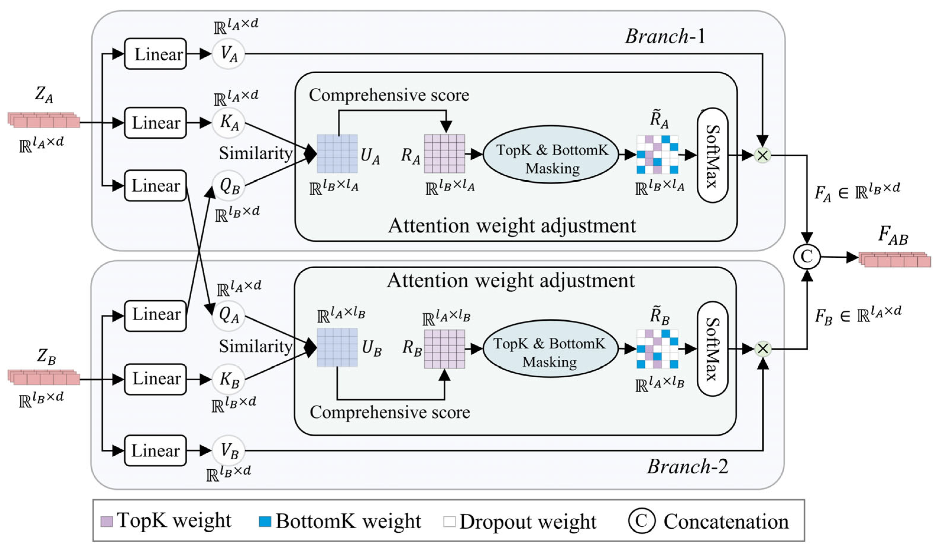
Multimodal features exhibit inherent complementarity and significant heterogeneity. On the one hand, not all information hidden in multimodal features is valuable, and interfering information (e.g., sensor noise) readily degrades fusion performance. On the other hand, while highly correlated multimodal information enhances feature representation, low-correlation yet discriminative details (e.g., sudden atmospheric pressure changes) are also critical for TC intensity prediction. However, existing cross-attention-based multimodal fusion methods assign weights solely based on inter-modal correlation and only prioritize highly correlated features, leading to biased feature representations and degraded model robustness. To this end, we propose a discriminative cross-fusion module (DisCF), which adopts information entropy to quantify cross-modal heterogeneity and information uncertainty, thereby providing solid theoretical support for adaptive feature screening. The architecture of DisCF is illustrated in Figure 4 and consists of two symmetric interaction branches. Through dual-branch interaction, both input modalities actively mine valuable complementary information from each other while retaining their inherent attribute characteristics, thus effectively boosting fused feature representations.

Given two inputs $Z_A=\left\{z_A^1, z_A^2,\dots , z_A^{l_A}\right\}\in {\mathbb{R}}^{l_A\times d}$ and $Z_B=\left\{z_B^1, z_B^2,\dots , z_B^{l_B}\right\}\in {\mathbb{R}}^{l_B\times d}$. In Branch 1, $Z_B$ serves as guidance feature to construct the query and mine valuable complementary information from $Z_A$. First, $Z_A$ and $Z_B$ are projected to $Q_B=Z_B{W}^Q$, $K_A=Z_A{W}^K$, and $V_A=Z_A{W}^V$, where $W^Q$, $W^V$, $W^K$ are learnable linear projection matrices. The cross-modal similarity matrix $U_A\in {\mathbb{R}}^{l_B\times l_A}$ is computed as:

$$U_A={\displaystyle \frac{Q_B{K}_A^{\mathrm{T}}}{\sqrt{d}}}$$

(13)

where $u_{ij}$ in $U_A$ denotes the similarity score between the i-th element in $Q_B$ and the j-th element in $K_A$. To effectively distinguish interfering information from valid feature information, we construct a comprehensive score matrix $R_A$ derived from $U_A$ by integrating feature similarity and information entropy. This integration balances inter-modal correlation and modal uncertainty, overcoming the inherent limitation of correlation-only fusion strategies. The score $r_{ij}$ in $R_A$ is formulated as:

$$r_{ij}=\alpha \left|u_{ij}\right|+\left(1-\alpha \right)H\left(U_{A,i}\right)$$

(14)

where $U_{A,i}$ denotes the i-th row of the similarity matrix $U_A$; $H\left(U_{A,i}\right)=-{\displaystyle {\sum }_{j=1}^{l_A}}{\widehat{u}}_{ij}\mathrm{l}\mathrm{o}\mathrm{g}{\widehat{u}}_{ij}$ is the information entropy of $U_{A,i}$, where ${\widehat{u}}_{ij}={\mathrm{S}\mathrm{o}\mathrm{f}\mathrm{t}\mathrm{M}\mathrm{a}\mathrm{x}\left(U_{A,i}\right)}_j$ denotes the row-wise normalized probability; and $\alpha \in \left(0, 1\right)$ is a balancing hyperparameter. An extremely small $r_{ij}$ represents pure noise or redundant interference with negligible valid information. A moderate $r_{ij}$ corresponds to low-correlation but physically discriminative features. A large $r_{ij}$ represents highly correlated complementary features with consistent modal semantics. Based on the hierarchical distribution of $r_{ij}$ scores, we construct a mask matrix $\mathcal{M}$ with the same dimension as $R_A$ to implement adaptive feature screening, and derive the attention weights as follows:

$${\tilde{R}}_A=\mathcal{M}+R_A$$

(15)

The element ${\mathcal{m}}_{ij}\in \mathcal{M}$ is defined by:

$${\mathcal{m}}_{ij}=\left\{\begin{array}{cc}\hfill 0,& r_{ij}\in {\mathrm{Topk}}_i\left(R_{A,i}\right)\hfill \\ \hfill 0,& r_{ij}\in {\mathrm{Bottomk}}_i\left(\mathrm{R}\mathrm{e}\mathrm{m}\mathrm{o}\mathrm{v}\mathrm{e}\left(R_{A,i},{ r}_{min}\right)\right)\hfill \\ \hfill -\infty ,& \mathrm{Otherwise}\hfill \end{array}\right.$$

(16)

where ${\mathrm{Topk}}_i\left(·\right)$ is the TopK operation selecting $k_i$ elements to retain high-correlation complementary features, improving multimodal representation consistency; $\mathrm{R}\mathrm{e}\mathrm{m}\mathrm{o}\mathrm{v}\mathrm{e}\left(R_{A,i}, r_{min}\right)$ filters out interference elements of $R_{A,i}$ below the threshold $r_{min}$ to eliminate pure noise with almost no effective information; $\mathrm{B}\mathrm{o}\mathrm{t}\mathrm{t}\mathrm{o}\mathrm{m}{\mathrm{k}}_i\left(·\right)$ is the BottomK operation selecting ${\mathit{k}}_i$ elements to preserve low-correlation but critical discriminative features, compensating for the information omission issue of traditional correlation-based fusion methods. The three operations coordinate with entropy constraints to achieve comprehensive and robust feature screening. Notably, to adapt to the dynamic uncertainty of multimodal data, $k_i$ is dynamically adjusted according to entropy magnitude, formulated as:

$$k_i=\max \left(\lfloor k_{base}H\left(U_{A,i}\right)\rfloor , k_{min}\right)$$

(17)

where $k_{base}$ and $k_{min}$ are the base value and minimum value of $k_i$ to avoid zero feature screening and invalid screening operations, respectively. The entropy of $U_{A,i}$ directly reflects the dispersion of cross-modal similarity values. A higher entropy indicates more dispersed information, requiring a larger $k_i$ to retain sufficient detailed information, while a lower entropy signals concentrated information, necessitating a smaller $k_i$ to suppress redundant contents. This dynamic $k_i$ mechanism enables adaptive information screening for diverse similarity distributions.

Finally, the output for Branch 1 is obtained as:

$$F_A=\mathrm{SoftMax}\left({\tilde{R}}_A\right)V_A$$

(18)

Branch 2 takes $Z_A$ as guidance to construct the query feature and generates the output $F_B$ following the same pipeline as Branch 1. Then, outputs of the two branches are concatenated along the sequence dimension to obtain the fusion result $F_{AB}=\mathrm{C}\mathrm{o}\mathrm{n}\mathrm{c}\mathrm{a}\mathrm{t}\left(F_A, F_B\right)\in {\mathbb{R}}^{\left({l_A+l}_B\right)\times d}$, which fully preserves the sequence features of both modalities without information compression loss.

Based on the DisCF, the same-timescale multimodal fusion result is expressed as follows:

$$F_m=\mathrm{DisCF}\left(\mathrm{DisCF}\left(Z_{N,m}, Z_{I,m}\right), Z_{T,m}\right)$$

(19)

where $\mathrm{DisCF}\left(·\right)$ denotes the function of DisCF, and $Z_{N,m}$, $Z_{I,m}$, $Z_{T,m}$ denote the numerical, satellite, and textual features at the m-th timescale, respectively.

4.3.2. Multimodal Feature Fusion Across All Timescales

In this section, the final multimodal fusion representation is generated by integrating the fusion results across all timescales. Since critical information contained in multi-timescale features differs significantly, small-timescale features capture local details (e.g., instantaneous fluctuations and sudden peaks), while large-timescale features depict global patterns (e.g., long-term trends and periodic variations) of TC intensity. To this end, this study adopts a hierarchical fusion strategy, which first performs weighted fusion on adjacent timescale pairs to produce intermediate results, and then aggregates all such intermediate results to form the final representation:

$$F_{MC}={\displaystyle {\sum }_{m=1}^{M-1}}{\beta }_m\left({\alpha }_m{F}_m+{\alpha }_{m+1}{F}_{m+1}\right)$$

(20)

where $F_m$ denotes the multimodal fusion result at the m-th timescale; ${\alpha }_m$ and ${\alpha }_{m+1}$ are learnable local coefficients used to modulate the contributions of adjacent paired timescale features; and ${\beta }_m$ is the learnable global coefficient for weighting the corresponding intermediate fusion results. This refined fusion strategy fully exploits the complementarity of multi-timescale features and provides reliable, comprehensive feature inputs for waypoint-level TC intensity prediction.

4.4. Denoising Network and Model Training Procedure

After obtaining the multimodal fusion results, this study uses the denoising network $z_{\theta }$ to predict the noise to be removed at each step, thereby obtaining waypoint-level TC intensity predictions. Due to the high real-time requirements of TC forecasting tasks, we adopt a fully connected network (FCN) as the denoising backbone to simplify network structure and reduce computational overhead. At denoising step k, the inputs of the denoising network include the noisy sample $Y_k^{t+n}$, denoising step k, and the multimodal condition $F_{MC}$. We first apply a linear transformation to each input and concatenate these transformed inputs to generate an intermediate representation. Then, we feed this representation into the FCN to output the predicted noise ${\tilde{z}}_k$. At this stage, the reverse denoising process is completed. Subsequently, we train the model using Equation (8). The overall training procedure is summarized in Algorithm 1.

Algorithm 1: The Training Procedure of MADiff

Input: total diffusion step K, total epoch number E, TC intensity dataset $D_{SI}$, multimodal dataset $D_{MC}$, model parameters $\theta$   Output: The trained MADiff model

1 for e = 1, …, E do

2  $Y_0^{t+n}\leftarrow$ Sample$\left(D_{SI}\right)$;

3  $\left(X_N, S_N, X_I, S_I, X_T,{ S}_T\right)\leftarrow$ ExtractMultimodalCondition$\left(D_{MC}\right)$;

4  $F_{MC}\leftarrow \mathrm{Fusion}\left(X_N, S_N, X_I, S_I, X_T,{ S}_T\right)$;

5  $k~\mathrm{Uniform}\left(\left\{1, 2, 3, ..., K\right\}\right)$;

6  $z_k~\mathcal{N}\left(\mathbf{0},\mathbf{I}\right)$;

7  $Y_k^{t+n}=\sqrt{{\overline{\alpha }}_k}{Y}_0^{t+n}+\sqrt{1-{\overline{\alpha }}_k}{z}_k$;

8  ${\mathcal{L}}_{total}={\mathcal{L}}_{diff}+{\lambda \mathcal{L}}_{phy}$;

9  Take gradient descent step on $\nabla {\mathcal{L}}_{total}$;

10 end

11 return $\theta$

4.5. MADiff-Based Waypoint-Level TC Intensity Prediction Procedure

After model training is completed, we can generate waypoint-level TC intensity predictions using Equation (3). Specifically, we first randomly sample $Y_K^{t+n}~\mathcal{N}\left(\mathbf{0},\mathbf{I}\right)$ from a standard Gaussian distribution with the same size as the target output. Then, via K-step reverse denoising, we obtain the corresponding waypoint-level TC intensity prediction $Y_0^{t+n}$. To improve prediction stability and reliability, we repeat the generation process G times and compute the average as the final output. The prediction procedure of the proposed MADiff is summarized in Algorithm 2.

Algorithm 2: The Prediction Procedure of MADiff

Input: total diffusion step K, total generation number G, multimodal dataset $D_{MC}$, well-trained model θ

Output: Waypoint-level TC intensity predictions $Y^{t+n}$

1 $\left(X_N, S_N, X_I, S_I, X_T,{ S}_T\right)\leftarrow$ ExtractMultimodalCondition$\left(D_{MC}\right)$;

2 $F_{MC}\leftarrow \mathrm{Fusion}\left(X_N, S_N, X_I, S_I, X_T,{ S}_T\right)$;

3 for $g=1, \dots , \mathrm{G}$ do

4   $Y_{K,g}^{t+n}~\mathcal{N}\left(\mathbf{0}, \mathbf{I}\right)$;

5   for $k=K, \dots , 1$ do

6   $z_k~\mathcal{N}\left(\mathbf{0},\mathbf{I}\right) \mathbf{i}\mathbf{f} k>1$, else $z_k=\mathbf{0}$;

7   $Y_{k-1,g}^{t+n}\leftarrow {\displaystyle \frac{1}{\sqrt{{\alpha }_k}}}\left(Y_{k,g}^{t+n}-{\displaystyle \frac{{\beta }_k}{\sqrt{1-{\overline{\alpha }}_k}}}{z}_{\theta }\left(Y_{k,g}^{t+n}, k, F_{MC}\right)\right)+{\sigma }_k{z}_k$;

8   end

9 end

10 return $Y^{t+n}\leftarrow {\displaystyle \frac{1}{G}}{\displaystyle {\sum }_{g=1}^G}{Y}_{0,g}^{t+n}$

5. Experiment

5.1. Experimental Setup

5.1.1. Datasets

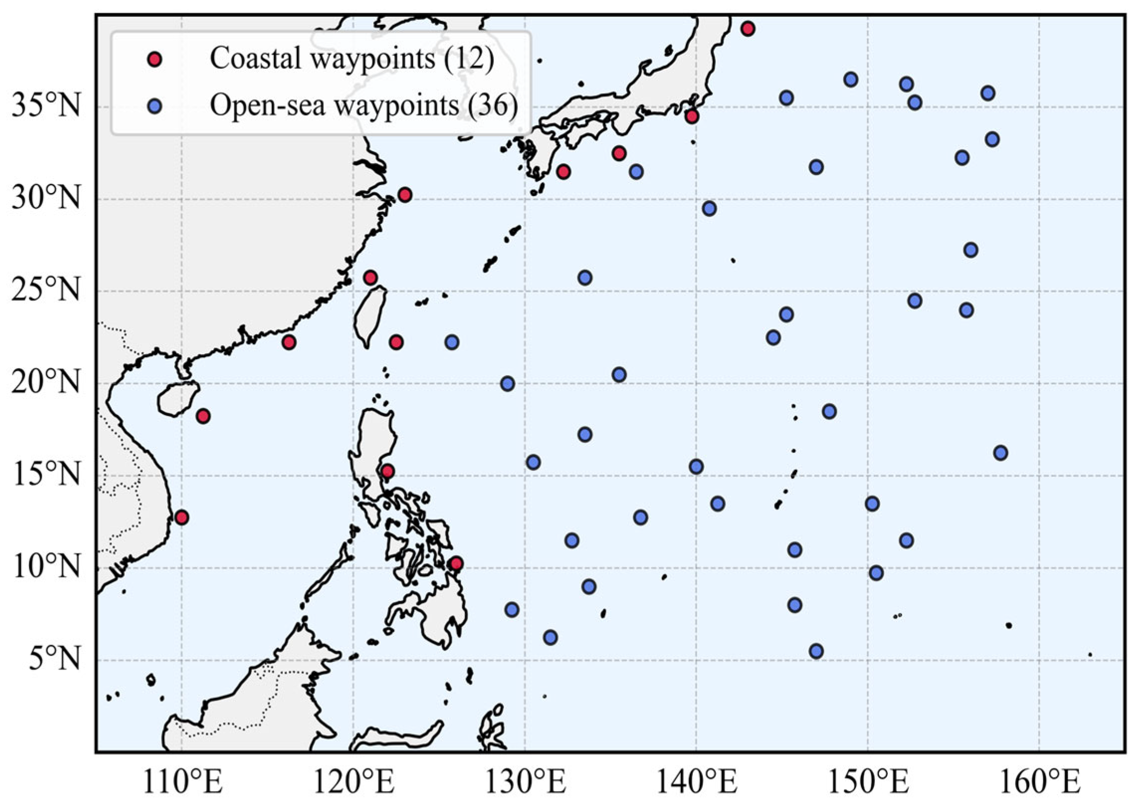
Maritime waypoints, TC records and multimodal data. To verify the applicability and effectiveness of the proposed MADiff in maritime transportation scenarios, this study selects 48 representative waypoints in the Western North Pacific, including 12 coastal waypoints (CWs) and 36 open-sea waypoints (OWs). The CWs are distributed across major ports and nearshore shipping lanes, while the OWs are distributed along key maritime routes. Detailed geographical coordinates of all selected waypoints are listed in

Table 2. Geographic coordinates of maritime waypoints.

Coastal Waypoints (CWs)		Open-Sea Waypoints (OWs)
ID	Coordinates (°E, °N)	ID	Coordinates (°E, °N)	ID	Coordinates (°E, °N)	ID	Coordinates (°E, °N)
1	111.25, 18.25	1	136.50, 31.50	13	140.75, 29.50	25	145.75, 11.00
2	116.25, 22.25	2	129.25, 7.75	14	130.50, 15.75	26	147.75, 18.50
3	121.00, 25.75	3	133.50, 25.75	15	140.00, 15.50	27	150.50, 9.75
4	123.00, 30.25	4	157.25, 33.25	16	131.50, 6.25	28	133.75, 9.00
5	122.50, 22.25	5	145.25, 35.50	17	144.50, 22.50	29	157.00, 35.75
6	122.00, 15.25	6	152.25, 11.50	18	150.25, 13.50	30	152.75, 24.50
7	126.00, 10.25	7	155.75, 24.00	19	125.75, 22.25	31	141.25, 13.50
8	139.75, 34.50	8	152.25, 36.25	20	135.50, 20.50	32	156.00, 27.25
9	132.25, 31.50	9	129.00, 20.00	21	147.00, 31.75	33	133.50, 17.25
10	110.00, 12.75	10	152.75, 35.25	22	145.25, 23.75	34	149.00, 36.50
11	143.00, 39.25	11	136.75, 12.75	23	132.75, 11.50	35	155.50, 32.25
12	135.50, 32.50	12	157.75, 16.25	24	147.00, 5.50	36	145.75, 8.00

. In addition, the spatial distribution of these waypoints is illustrated in Figure 5 to demonstrate their overall layout.

Subsequently, we collect 219 historical TC records across the Western North Pacific for the period from 1 January 2015 to 31 December 2022. These records are obtained from the CMA Best Track Dataset (CMA_BT) [35,36]. Meanwhile, we obtain multimodal data for the 48 selected waypoints covering the same period. Detailed information on the multimodal data is presented in Section 3.1. In situ wind observations over open-ocean waypoints are highly sparse, and satellite wind retrievals only yield intermittent spatiotemporal snapshots that cannot support continuous sequential forecasting. Accordingly, hourly sustained wind speeds extracted from the ERA5 reanalysis dataset are adopted as the reference labels for waypoint-level TC intensity prediction.

Dataset construction. To fully verify the generalization capability of the proposed MADiff, we construct four datasets corresponding to coastal and open-sea regions. These datasets are denoted as Coastal-S, Open-S, Coastal-US, and Open-US, where S denotes seen waypoints used in training, while US denotes unseen waypoints never observed during training. Specifically, Coastal-S and Open-S are used to evaluate the performance of our MADiff on seen waypoints, while Coastal-US and Open-US are employed to test the generalization ability on unseen waypoints in the two regions. For training and validation, all datasets use the same waypoints (CW1-8 and OW1-24). The test set is designed to evaluate generalization across different regions and unseen waypoints. In each dataset, we employ a sliding window strategy to construct samples, where 24 h of historical multimodal data are used to predict the waypoint-level TC intensity for the next 12 h, with a sliding step of 6 h. The details of the time spans, TC counts, sample counts, and waypoints for the training, validation, and test sets across each of the four datasets are presented in

Table 3. Dataset details.

Subset	Category	Coastal-S	Open-S	Coastal-US	Open-US
Training set	Time span	1 January 2015, to 31 December 2019
	Waypoint	CW1-8, OW1-24
	TC count	138
	TC identity	TC1-TC138
	Sample count	54,400
Validation set	Time span	1 January 2020, to 31 December 2020
	Waypoint	CW1-8, OW1-24
	TC count	26
	TC identity	TC139-TC164
	Sample count	11,680
Test set	Time span	1 January 2021, to 31 December 2022
	Waypoint	CW1-8	OW1-24	CW9-12	OW25-36
	TC count	55
	TC identity	TC165-TC219
	Sample count	2920	8760	1460	4380

.

5.1.2. Implementation Details

For data preprocessing, min-max normalization is applied to all numerical meteorological features to scale values into the range [0, 1]. All normalization parameters are calculated solely based on the training set, and the same parameters are applied to the validation and test sets to avoid data leakage. Infrared satellite images and text features are preprocessed by their respective pre-trained encoders (MobileNetV2 for imagery and TinyBERT for text) without additional normalization.

The Adam optimizer with β₁ = 0.9 and β₂ = 0.999 is employed for model training. The model is trained for a maximum of 100 epochs, and an early stopping strategy is adopted to terminate training when the validation loss exhibits no significant improvement for 10 consecutive epochs. The initial learning rate is set to 1 × 10⁻⁴, and the learning rate is decayed by a factor of 0.1 every 10 epochs. A training batch size of 16 is adopted, and L2 regularization with a coefficient of 0.0001 is applied to all trainable parameters to alleviate overfitting. No dropout layer is adopted in the model, and overfitting is jointly constrained by L2 regularization and early stopping strategy.

In terms of network dimensions, the timestamp embedding dimension is set to 32 for encoding the periodic temporal information of multimodal data, and the diffusion timestep embedding dimension is set to 32. All other hidden layers across the entire model adopt a unified hidden dimension of 64, including the modality projection layers, the TDConv module, the DisCF module, and the fully connected layers of the denoising network.

The TDConv module adopts the triple-scale kernel combination (6, 12, 18) for temporal feature extraction. The DisCF module has an entropy balance coefficient of 0.5. The noise filtering threshold of the DisCF module is configured as 0.08 to filter noisy features, and the minimum and base values for the dynamic TopK/BottomK selection mechanism are set to 2 and 3, respectively.

For the diffusion model configuration, the total diffusion step is set to 200 to control the denoising level. We adopt a standard linear noise schedule, where the noise variance β increases linearly from 10⁻⁴ at the first step to 0.02 at the last step. During inference, the number of generation rounds is fixed at 8 for output stability.

All experiments are implemented with the PyTorch 2.9 framework and run on an NVIDIA GeForce RTX 3080 GPU. We utilize different random seeds (0, 1, 2, 3, 4) to conduct the experiments five times and report the mean and standard deviation.

5.1.3. Evaluation Metrics

Mean Absolute Error (MAE), Root Mean Square Error (RMSE), and Continuous Ranked Probability Score (CRPS) are employed as the evaluation metrics to assess the predictive performance of the proposed MADiff. MAE and RMSE quantify the average absolute deviation between the predicted values and the ground truth, while CRPS evaluates the consistency between the estimated probabilistic distribution and the observed ground-truth values.

$$MAE={\displaystyle \frac{1}{B}}{\displaystyle {\sum }_{b=1}^B}\left|{\widehat{y}}_b-y_b\right|$$

(21)

$$RMSE=\sqrt{{\displaystyle \frac{1}{B}}{\displaystyle {\sum }_{b=1}^B}{\left({\widehat{y}}_b-y_b\right)}^2}$$

(22)

$$CRPS={\displaystyle \frac{1}{B}}{\displaystyle {\sum }_{b=1}^B}\left({\displaystyle \frac{1}{G}}{\displaystyle {\sum }_{g=1}^G}\left|x_{b,g}-y_b\right|-{\displaystyle \frac{1}{2G^2}}{\displaystyle {\sum }_{g=1}^G}{\displaystyle {\sum }_{m=1}^G}\left|x_{b,g}-x_{b,m}\right|\right)$$

(23)

Here, $B$ denotes the total number of test samples, $G$ is the generation number, ${\widehat{y}}_b$ is the predicted value, $y_b$ is the corresponding ground truth, and $x_{b,g}$ denotes the g-th sample drawn from the predictive distribution for the b-th test sample.

5.2. Comparison with the State-of-the-Art Baselines

To validate the effectiveness of the proposed MADiff, we compare it with 10 representative baselines, which are divided into three groups according to their inputs.

Unimodal baselines: ConvLSTM [41] uses satellite imagery as input. GRU [9], Informer [10], ARIMA [42], and TimeGrad [43] adopt only numerical data as inputs.

Dual-modal baselines: TCIP-Net [17], MSCAR [18], TC-Diffuser [44], TCIF-fusion [45], and TC-Clouds-DP [46] are multimodal approaches that take both satellite imagery and numerical data as inputs. To ensure a fair comparison under identical input and preprocessing settings, we design a dual-modal variant termed MADiff-NS, which uses exactly the same two modalities and data processing pipelines as these baselines.

All-modal MADiff: The MADiff further incorporates TC-related text data on the basis of dual-modal inputs. The comparison between MADiff and MADiff-NS quantifies the performance gain brought by the introduction of the additional text modality.

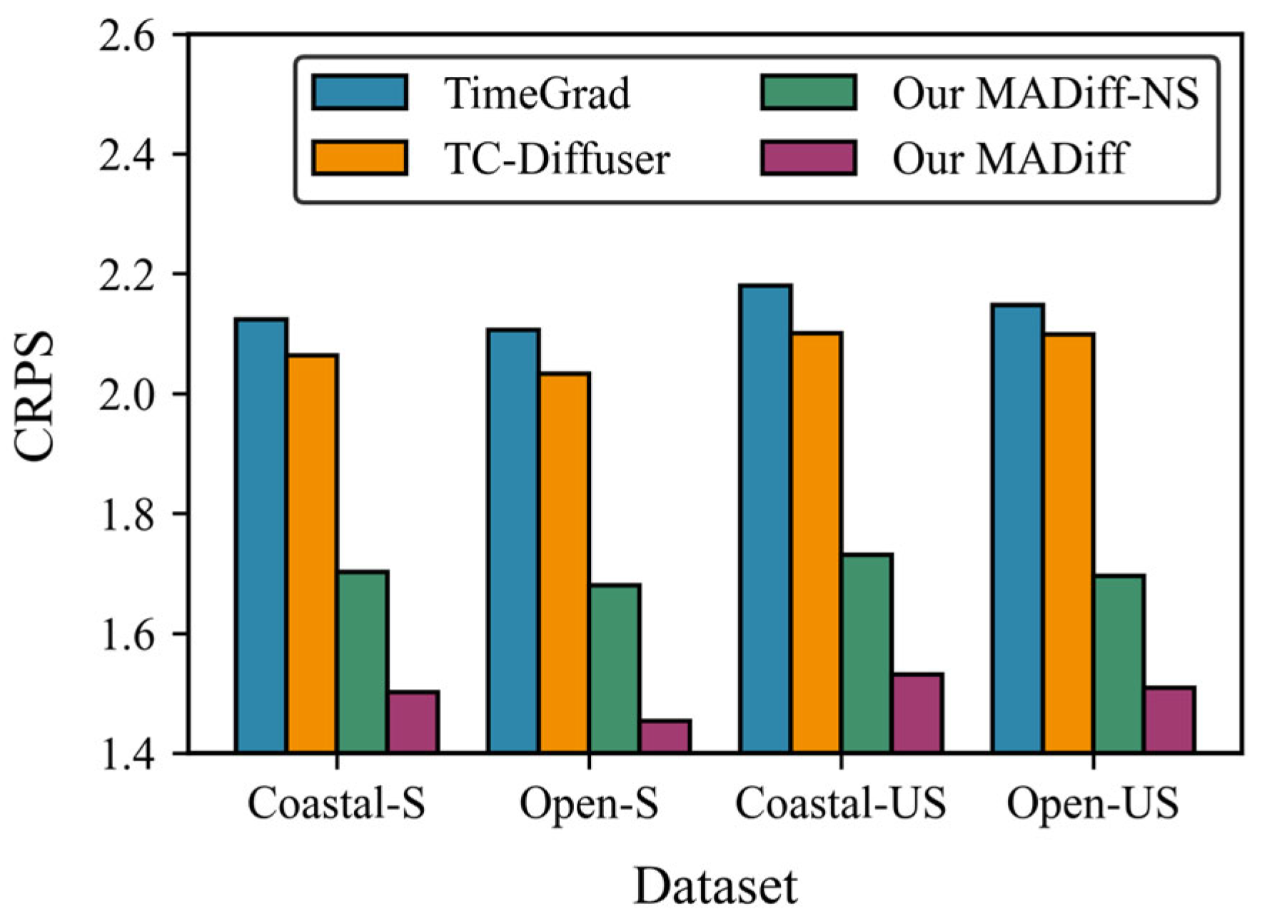
For probabilistic forecasting methods, including TimeGrad, TC-Diffuser, MADiff-NS, and MADiff, we generate 100 prediction samples to characterize the predictive probability distribution. We evaluate these distributions using the CRPS metric for quantitative evaluation, and take the sample mean as the deterministic prediction.

Table 4. Experimental results compared with different baselines.

Input	Method	Coastal-S		Open-S		Coastal-US		Open-US
		MAE	RMSE	MAE	RMSE	MAE	RMSE	MAE	RMSE
Unimodal	ConvLSTM	2.66 ± 0.19	2.88 ± 0.22	2.65 ± 0.18	2.86 ± 0.22	2.68 ± 0.21	2.93 ± 0.23	2.67 ± 0.20	2.91 ± 0.22
	ARIMA	3.51 ± 0.35	3.80 ± 0.41	3.50 ± 0.33	3.69 ± 0.38	3.65 ± 0.38	3.88 ± 0.42	3.64 ± 0.36	3.87 ± 0.41
	GRU	2.70 ± 0.17	3.04 ± 0.20	2.68 ± 0.15	2.89 ± 0.19	2.83 ± 0.19	3.11 ± 0.20	2.79 ± 0.17	3.05 ± 0.19
	Informer	2.44 ± 0.13	2.65 ± 0.15	2.41 ± 0.12	2.61 ± 0.15	2.53 ± 0.15	2.66 ± 0.16	2.50 ± 0.15	2.61 ± 0.17
	TimeGrad	2.52 ± 0.29	2.70 ± 0.31	2.50 ± 0.26	2.71 ± 0.29	2.60 ± 0.30	2.87 ± 0.33	2.55 ± 0.26	2.79 ± 0.31
Dual-modal	MSCAR	2.61 ± 0.16	2.79 ± 0.16	2.59 ± 0.15	2.77 ± 0.16	2.65 ± 0.18	2.89 ± 0.19	2.63 ± 0.17	2.86 ± 0.19
	TCIP-Net	2.56 ± 0.13	2.79 ± 0.15	2.53 ± 0.13	2.81 ± 0.15	2.62 ± 0.14	2.89 ± 0.15	2.60 ± 0.13	2.84 ± 0.13
	TCIF-fusion	2.51 ± 0.15	2.73 ± 0.18	2.47 ± 0.13	2.70 ± 0.17	2.59 ± 0.15	2.75 ± 0.19	2.53 ± 0.15	2.71 ± 0.17
	TC-Diffuser	2.49 ± 0.27	2.65 ± 0.30	2.45 ± 0.25	2.59 ± 0.29	2.53 ± 0.29	2.71 ± 0.31	2.50 ± 0.26	2.69 ± 0.27
	TC-Clouds-DP	2.45 ± 0.10	2.62 ± 0.12	2.41 ± 0.10	2.53 ± 0.11	2.50 ± 0.13	2.68 ± 0.15	2.47 ± 0.13	2.63 ± 0.15
	MADiff-NS	2.32 ± 0.08	2.50 ± 0.09	2.25 ± 0.07	2.41 ± 0.07	2.39 ± 0.09	2.61 ± 0.10	2.37 ± 0.09	2.56 ± 0.09
All-modal	MADiff	2.07 ± 0.07 *	2.31 ± 0.06 *	2.05 ± 0.06 *	2.30 ± 0.06 *	2.10 ± 0.07 *	2.45 ± 0.07 *	2.08 ± 0.07 *	2.41 ± 0.07 *

* denotes statistical significance (p < 0.05) compared to the best baseline TC-Clouds-DP.

summarizes the experimental results in terms of MAE and RMSE, and Figure 6 reports the CRPS scores. Experimental results demonstrate that MADiff outperforms all baselines across all datasets. Notably, under the same dual-modal input setting, MADiff-NS consistently outperforms all existing dual-modal baselines on all four datasets. This result fully demonstrates that our proposed architectural innovations (TDConv for multi-timescale feature alignment, DisCF for discriminative cross-modal fusion, and physics-constrained diffusion modeling) can effectively exploit multimodal information and bring significant performance improvements that are independent of data volume. After further introducing the TC-related text modality, the full MADiff model achieves substantial further performance improvement on the basis of MADiff-NS. For example, on the Coastal-S dataset, MAE decreases from 2.32 kt to 2.07 kt, which verifies that the text modality containing TC global state and relative position information has strong complementary value, and our DisCF module can effectively integrate cross-modal information to tap the potential of multi-modal data.

5.3. Performance Across Diverse Scenarios

To validate the performance of the proposed MADiff over different forecast lengths, this experiment sets multiple prediction intervals to meet maritime transportation requirements for short-term to long-term TC intensity forecasts. The experimental results are presented in

Table 5. Experimental results at different forecast lengths.

Forecast Lengths	Coastal-S		Open-S		Coastal-US		Open-US
	MAE	RMSE	MAE	RMSE	MAE	RMSE	MAE	RMSE
3 h	1.67 ± 0.06	1.86 ± 0.06	1.66 ± 0.06	1.84 ± 0.07	1.71 ± 0.07	1.88 ± 0.09	1.70 ± 0.08	1.86 ± 0.08
6 h	1.77 ± 0.06	1.97 ± 0.05	1.75 ± 0.06	1.93 ± 0.06	1.83 ± 0.09	2.10 ± 0.09	1.81 ± 0.08	2.06 ± 0.08
9 h	1.90 ± 0.07	2.23 ± 0.06	1.95 ± 0.08	2.17 ± 0.07	2.09 ± 0.10	2.28 ± 0.11	2.07 ± 0.09	2.13 ± 0.10
12 h	2.07 ± 0.07	2.31 ± 0.06	2.05 ± 0.06	2.30 ± 0.06	2.10 ± 0.07	2.45 ± 0.07	2.08 ± 0.07	2.41 ± 0.07
15 h	2.26 ± 0.07	2.64 ± 0.08	2.19 ± 0.06	2.58 ± 0.06	2.28 ± 0.08	2.68 ± 0.08	2.24 ± 0.07	2.60 ± 0.06
18 h	2.36 ± 0.07	2.81 ± 0.09	2.33 ± 0.07	2.75 ± 0.07	2.41 ± 0.10	2.83 ± 0.12	2.38 ± 0.09	2.80 ± 0.10
21 h	2.70 ± 0.09	3.15 ± 0.10	2.66 ± 0.09	3.13 ± 0.10	2.84 ± 0.13	3.29 ± 0.14	2.77 ± 0.10	3.31 ± 0.13
24 h	2.85 ± 0.11	3.29 ± 0.12	2.82 ± 0.10	3.22 ± 0.11	2.90 ± 0.15	3.38 ± 0.16	2.88 ± 0.12	3.32 ± 0.15

. For short-term forecasting tasks (e.g., 3 h, 6 h), both MAE and RMSE remain consistently low. These findings confirm that the proposed MADiff can effectively capture dynamic short-term trends in TC-related marine conditions. As forecast lengths extend (e.g., 12 h and beyond), both metrics exhibit a gradual upward trend. This is because waypoint-level TC evolution is governed by complex nonlinear factors such as atmospheric circulation and ocean currents. Longer prediction lengths amplify the cumulative effects of environmental uncertainties, increasing forecasting difficulty. Nevertheless, the MAE and RMSE of the proposed MADiff remain below 3 kt and 3.5 kt, respectively, which validates its high prediction accuracy and stability.

To further verify the model performance, we conduct stratified error analysis from three dimensions including TC intensity, cyclone evolution phase, and waypoint distance from the cyclone center. First, to evaluate model performance across different TC intensity levels, we classify all test samples into three intensity tiers based on the maximum sustained wind speed of the TC center ($V_{\mathrm{m}\mathrm{a}\mathrm{x}}$), following the official TC classification standard of the China Meteorological Administration: weak level ($V_{\mathrm{m}\mathrm{a}\mathrm{x}}$ < 48 kt), medium level (48 kt ≤ $V_{\mathrm{m}\mathrm{a}\mathrm{x}}$ ≤ 80 kt), and strong level ($V_{\mathrm{m}\mathrm{a}\mathrm{x}}$ ≥ 81 kt). Furthermore, to evaluate model performance under different cyclone evolution phases, we classify all test samples into three evolution phases based on the 24 h change in maximum sustained wind speed ($∆V_{\mathrm{m}\mathrm{a}\mathrm{x}}$), per standard international definitions for tropical cyclone intensity change: rapid intensification ($∆V_{\mathrm{m}\mathrm{a}\mathrm{x}}$ ≥ 30 kt), rapid weakening ($∆V_{\mathrm{m}\mathrm{a}\mathrm{x}}$≤ −30 kt), and steady variation (all remaining cases). Finally, to evaluate model performance at different positions relative to the cyclone core, we classify all test samples into three groups according to the great-circle distance between the waypoint and the TC center ($D_{wt}$). Considering the average scale of TCs in the Western North Pacific, the three groups include short distance ($D_{wt}$ < 150 km), medium distance (150 km ≤ $D_{\mathrm{m}\mathrm{a}\mathrm{x}}$ < 350 km), and long distance ($D_{wt}$ ≥ 350 km).

The experimental results are presented in

Table 6. Stratified error analysis under different TC scenarios.

Scenarios	Category	Coastal-S		Open-S		Coastal-US		Open-US
		MAE	RMSE	MAE	RMSE	MAE	RMSE	MAE	RMSE
TC central intensity	Weak level	1.74 ± 0.06	2.01 ± 0.05	1.68 ± 0.05	1.96 ± 0.05	1.82 ± 0.06	2.19 ± 0.06	1.77 ± 0.06	2.13 ± 0.06
	Medium level	2.02 ± 0.07	2.25 ± 0.06	2.00 ± 0.06	2.23 ± 0.06	2.05 ± 0.07	2.39 ± 0.07	2.03 ± 0.07	2.35 ± 0.07
	Strong level	2.51 ± 0.09	2.73 ± 0.07	2.40 ± 0.08	2.63 ± 0.07	2.56 ± 0.09	2.88 ± 0.08	2.49 ± 0.09	2.79 ± 0.08
TC evolution Phase	Rapid Intensification	2.55 ± 0.09	2.79 ± 0.08	2.46 ± 0.09	2.72 ± 0.08	2.64 ± 0.10	3.00 ± 0.09	2.56 ± 0.10	2.90 ± 0.09
	Rapid Weakening	2.23 ± 0.08	2.46 ± 0.07	2.18 ± 0.07	2.42 ± 0.07	2.28 ± 0.08	2.62 ± 0.07	2.24 ± 0.08	2.56 ± 0.07
	Steady variation	2.03 ± 0.07	2.27 ± 0.06	2.01 ± 0.06	2.25 ± 0.06	2.07 ± 0.07	2.42 ± 0.07	2.04 ± 0.07	2.37 ± 0.07
Distance from waypoint to TC center	Short distance	2.56 ± 0.09	2.78 ± 0.07	2.44 ± 0.08	2.69 ± 0.07	2.60 ± 0.09	2.95 ± 0.08	2.52 ± 0.09	2.85 ± 0.08
	Medium distance	2.02 ± 0.07	2.24 ± 0.06	2.01 ± 0.06	2.22 ± 0.06	2.06 ± 0.07	2.39 ± 0.07	2.03 ± 0.07	2.34 ± 0.07
	Long distance	1.80 ± 0.06	2.04 ± 0.05	1.76 ± 0.05	2.01 ± 0.05	1.87 ± 0.06	2.21 ± 0.06	1.82 ± 0.06	2.15 ± 0.06

. Prediction errors rise consistently with stronger TC center intensity, during rapid intensification phases, and for waypoints closer to the TC center. Specifically, stronger TC intensity is associated with more dramatic wind field structure changes, which increase fluctuations and nonlinearity in local waypoint wind speeds and raise forecasting difficulty. During rapid intensification, the TC undergoes rapid internal dynamic restructuring, and local wind speeds at waypoints show sharp non-stationary variations. Greater cross-modal heterogeneity and uncertainty in multimodal observations further complicate temporal modeling and cross-modal fusion. In terms of distance from the TC center, waypoints near the core eyewall region have steeper wind speed gradients and more complex turbulent flow structures, which naturally lead to higher forecasting difficulty. Overall, MADiff maintains consistent performance advantages across all high-risk scenarios, including strong intensity levels, rapid intensification phases and near-core regions. This robust forecasting capability provides reliable support for fine-grained maritime navigation safety assessment and route planning.

5.4. Ablation Study

5.4.1. Ablation Study of Multimodal Input Combinations

To systematically evaluate the effectiveness of different multimodal input combinations for the proposed MADiff, we conduct comprehensive ablation studies with single-modal, dual-modal, and all-modal input configurations including numerical meteorological data, infrared satellite imagery, and TC-related texts. Specifically, single-modal setups use only one of these modalities, dual-modal setups fuse any two of them, and the all-modal setup simultaneously integrates all three modalities.

Table 7. Experimental results of different multimodal combinations.

Numerical Data	Satellite Imagery	TC-Related Texts	Coastal-S		Open-S		Coastal-US		Open-US		Trainable Parameters (K)	Inference Time (s)
			MAE	RMSE	MAE	RMSE	MAE	RMSE	MAE	RMSE
√			3.04 ± 0.10	3.13 ± 0.11	2.99 ± 0.10	3.06 ± 0.11	3.20 ± 0.13	3.40 ± 0.15	3.13 ± 0.11	3.39 ± 0.14	147.97	0.003010
	√		4.31 ± 0.15	4.69 ± 0.16	4.15 ± 0.13	4.39 ± 0.15	4.51 ± 0.24	4.83 ± 0.26	4.49 ± 0.20	4.63 ± 0.22	165.26	0.003038
		√	5.44 ± 0.21	5.61 ± 0.22	5.09 ± 0.18	5.32 ± 0.20	5.56 ± 0.25	5.70 ± 0.26	5.56 ± 0.24	5.69 ± 0.26	173.45	0.003052
√	√		2.32 ± 0.08	2.50 ± 0.09	2.25 ± 0.07	2.41 ± 0.07	2.39 ± 0.09	2.61 ± 0.10	2.37 ± 0.09	2.56 ± 0.09	269.93	0.003216
√		√	2.55 ± 0.09	2.71 ± 0.10	2.50 ± 0.08	2.86 ± 0.11	2.73 ± 0.11	3.16 ± 0.12	2.70 ± 0.10	3.12 ± 0.11	278.12	0.003230
	√	√	4.43 ± 0.13	4.53 ± 0.15	4.06 ± 0.11	4.32 ± 0.13	4.51 ± 0.14	4.70 ± 0.17	4.43 ± 0.14	4.63 ± 0.16	294.41	0.003258
√	√	√	2.07 ± 0.07	2.31 ± 0.06	2.05 ± 0.06	2.30 ± 0.06	2.10 ± 0.07	2.45 ± 0.07	2.08 ± 0.07	2.41 ± 0.07	399.08	0.003435

presents the experimental results, which demonstrate that the all-modal scheme significantly outperforms both single-modal and dual-modal schemes.

Notably, single-modal setups exhibit subpar performance due to insufficient input information, whereas dual-modal setups are constrained by insufficient complementarity among the selected modalities. For instance, combining numerical meteorological data with TC-related texts can lead to the loss of critical spatial morphological features. In contrast, the all-modal framework integrates the quantitative precision of numerical data, spatial morphological details from satellite imagery, and semantic context from TC texts, thereby enabling a more comprehensive characterization of the dynamic evolution patterns of TCs. This synergistic integration improves the robustness of MADiff to environmental disturbances, thereby achieving more reliable predictive performance.

5.4.2. Ablation Study of Key Components

This section validates the effectiveness of each key component in MADiff for waypoint-level TC intensity prediction through ablation experiments. Specifically, we compare the full MADiff with the following four variants:

• w/o TDConv: Remove the TDConv module and replace it with standard 1D convolution.
• w/o DisCF: Remove the DisCF module and replace it with standard cross-attention fusion.
• w/o Diff: Remove the diffusion model and replace it with a multi-layer perceptron (MLP).
• w/o PhyLoss: Remove the physics-informed loss from the overall training objective.

The experimental results are shown in

Table 8. Ablation results of key components in terms of MAE.

Variants	Coastal-S	Open-S	Coastal-US	Open-US	Trainable Parameters (K)	Inference Time (s)
MADiff	2.07 ± 0.07	2.05 ± 0.06	2.10 ± 0.07	2.08 ± 0.07	399.08	0.003435
w/o TDConv	3.30 ± 0.12	3.27 ± 0.13	3.46 ± 0.15	3.29 ± 0.16	196.33	0.003167
w/o DisCF	3.67 ± 0.17	3.53 ± 0.15	3.70 ± 0.20	3.68 ± 0.19	390.97	0.003368
w/o Diff	3.44 ± 0.15	3.31 ± 0.14	3.67 ± 0.17	3.50 ± 0.17	396.97	0.000680
w/o PhyLoss	2.29 ± 0.12	2.16 ± 0.11	2.41 ± 0.15	2.40 ± 0.13	399.08	0.003435

. As observed across all datasets, all variants exhibit significant performance degradation compared with the complete MADiff model. This consistent phenomenon fully demonstrates the effectiveness of each proposed core module. For the w/o TDConv variant, removing TDConv fails to capture multi-timescale temporal dependencies and cannot adapt to multimodal inputs with distinct sampling intervals. The w/o DisCF variant lacks the ability to measure cross-modal heterogeneity, thereby being unable to filter redundant interference and extract useful modal features. Without the diffusion module, the w/o Diff variant loses strong probabilistic modeling capacity, and thus cannot characterize the inherent uncertainty of complex marine environments. The w/o PhyLoss variant exhibits noticeable performance degradation, especially on long-horizon forecasts and rapid intensification samples. This indicates that the physics-informed regularization term can effectively constrain unreasonable intensity mutations, thus improving the robustness of predictions. In summary, TDConv, DisCF, conditional diffusion and physics-informed loss make distinct contributions. The combination and synergy of these four core designs enable MADiff to achieve accurate and stable waypoint-level TC intensity prediction.

5.5. Hyperparameter Analysis

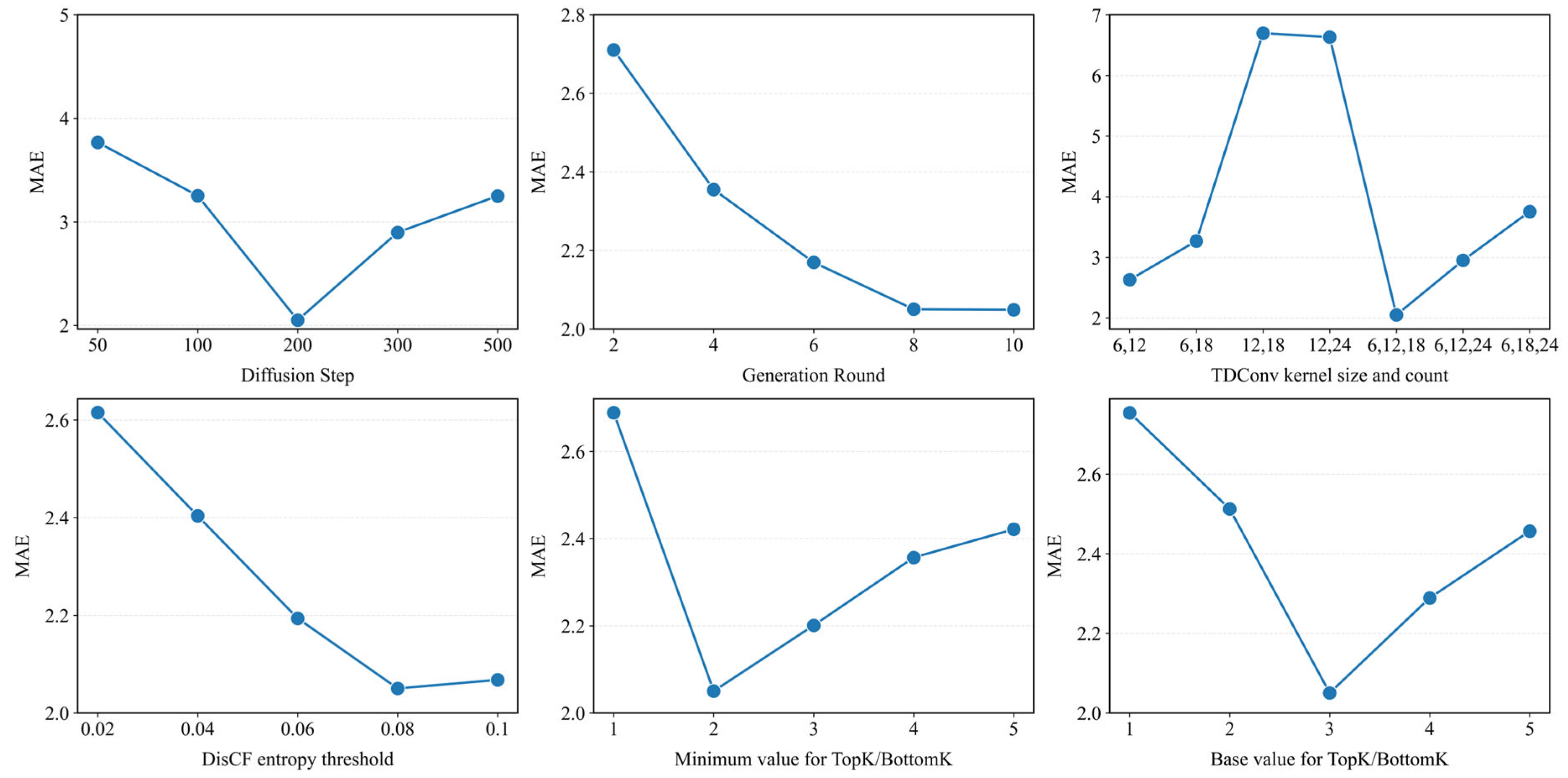
In this section, we analyze six key hyperparameters based on the Coastal-S dataset as a representative experimental scenario. All hyperparameter selections are determined solely on the validation set, and the test set is never accessed during model tuning to avoid data leakage. We apply the identical set of hyperparameters to all four datasets without any dataset-specific optimization. The experimental results are shown in Figure 7.

The diffusion step controls the denoising level during model inference. Both excessively large and small values degrade prediction performance. According to the results in Figure 7, we set the diffusion step to 200. The number of generation rounds governs the stability of model outputs. More rounds can reduce random fluctuations but increase computational overhead. As observed in Figure 7, we set this number to 8.

The TDConv kernel combination determines the capability of temporal feature extraction. Improper kernel scales fail to capture effective temporal patterns or introduce excessive noise interference. As shown in Figure 7, we employ the triple-scale combination (6, 12, 18).

The DisCF entropy threshold regulates the filtering of weak and noisy features. Inappropriate threshold values prevent the model from effectively retaining discriminative information. From the results in Figure 7, we set the DisCF entropy threshold to 0.08. The minimum value for TopK/BottomK defines the lower bound of retained features. A small value leads to insufficient feature preservation, while a large value introduces feature redundancy. Guided by Figure 7, we set this value to 2. The base value for TopK/BottomK adjusts the adaptive range of feature retention. An inappropriate value degrades the performance of adaptive feature selection. Based on Figure 7, we set this value to 3.

The coordinated configuration of these hyperparameters achieves a favorable balance among prediction accuracy, model stability, and computational efficiency.

5.6. Generalization Performance for Unseen Ocean Basins

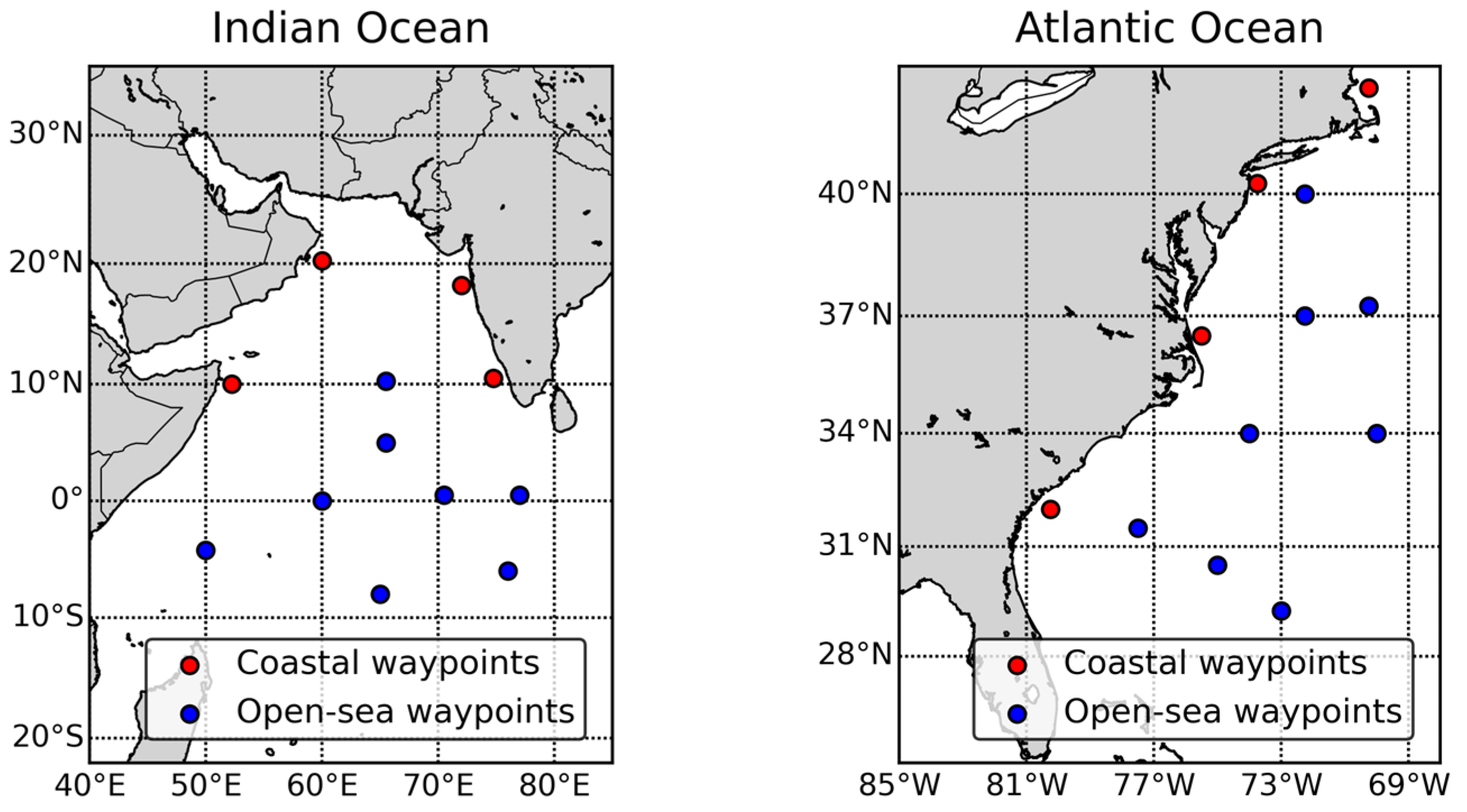
To evaluate the generalization ability of the proposed MADiff toward unseen ocean basins, we conduct cross-basin generalization experiments on the Atlantic and Indian Oceans. For each basin, we select 4 coastal and 12 open-sea waypoints as independent test sites, with their spatial distribution visualized in Figure 8. The model is trained exclusively on data from the Western North Pacific Ocean, without incorporating any samples from the Atlantic or Indian Oceans during training. The experimental results are presented in

Table 9. Generalization performance in the Indian and Atlantic Oceans.

Region	Forecast Lengths	Coastal Waypoints		Open-Sea Waypoints
		MAE	RMSE	MAE	RMSE
Atlantic Ocean	12 h	2.29 ± 0.10	2.61 ± 0.13	2.25 ± 0.09	2.59 ± 0.12
	24 h	3.10 ± 0.11	3.53 ± 0.13	3.07 ± 0.10	3.43 ± 0.12
Indian Ocean	12 h	2.24 ± 0.09	2.59 ± 0.11	2.31 ± 0.13	2.53 ± 0.13
	24 h	3.26 ± 0.13	3.77 ± 0.15	3.20 ± 0.13	3.61 ± 0.13

. Across both ocean basins, prediction performance is comparable for coastal and open-sea waypoints. Although the model performs marginally better in the Atlantic Ocean than in the Indian Ocean, this performance gap is particularly evident for 24 h forecasts. Nevertheless, it maintains reliable predictive accuracy in both basins. These cross-basin results confirm that MADiff exhibits strong generalization capability toward unseen ocean basins, verifying its promising applicability for practical deployment.

5.7. Calibration and Reliability Analysis

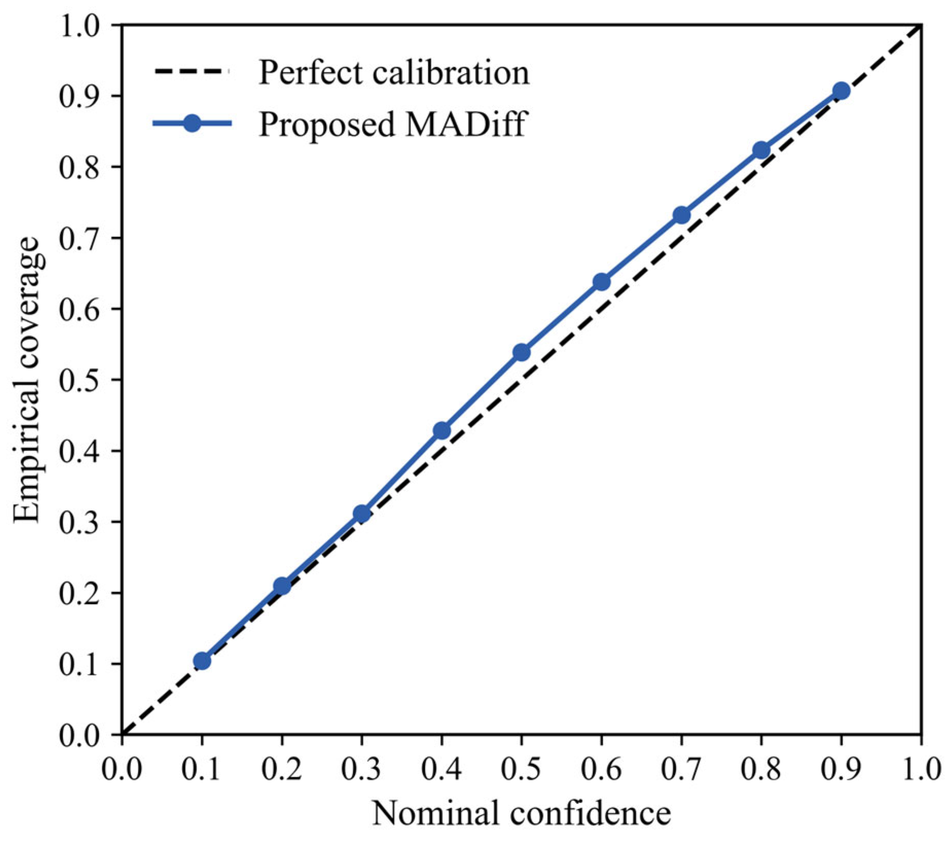
Different from CRPS-based quantitative comparison, this section emphasizes the uncertainty calibration and prediction reliability of the proposed MADiff to verify its practical performance for TC intensity forecasting. We systematically evaluate the model from multiple perspectives, including the 95% prediction interval, interval coverage rate, expected calibration error (ECE), and reliability diagram. All results are reported as the average across all four datasets. MADiff produces a physically reasonable 95% prediction interval ranging from 7.7313 kt to 22.8875 kt. The corresponding interval coverage reaches 94.12%, which is very close to the nominal 95% confidence level and reflects good overall calibration performance. This slight undercoverage falls within an acceptable range for maritime safety forecasting, ensuring stable uncertainty quantification. Meanwhile, the low ECE value of 0.0215 further confirms the superior calibration accuracy of MADiff, with only a minor mismatch between predicted confidence and observed probability. The reliability diagram is illustrated in Figure 9, where the dashed diagonal line denotes the ideal perfect calibration state. The calibration curve of MADiff closely aligns with the diagonal, which is consistent with the low ECE and the near-nominal coverage rate of the 95% prediction interval. Collectively, these quantitative results demonstrate that MADiff achieves accurate, stable and reliable uncertainty estimation, supporting trustworthy waypoint-level TC intensity prediction for real-world marine application scenarios.

5.8. Time Complexity

We further analyze the time complexity of the core MADiff framework, excluding frozen pre-trained image and text encoders (treated as fixed overhead). In the multimodal preprocessing stage, for a mini-batch containing B samples, the complexity is dominated by the linear projection of numerical meteorological data, denoted as $O\left(BLd\right)$. In the multimodal multi-timescale feature extraction and cross-fusion stage, the TDConv extracts multi-timescale unimodal features, while the DisCF module performs discriminative cross-modal fusion at each timescale. For a single timescale, TDConv yields a complexity of $O\left(BLd\right)$, and DisCF achieves a complexity of $O\left(BL{d}^2\right)$. Accordingly, the total complexity for M timescales is $O\left(BLd+BLM{d}^2\right)$. The final multi-timescale feature fusion only involves linear weighting, with negligible complexity $O\left(BMd\right)$. Thus, the overall complexity of this feature fusion stage is $O\left(BLM{d}^2\right)$. In the conditional diffusion denoising stage, the diffusion model performs K-step reverse denoising and averages G independent generation results to obtain stable waypoint-level TC intensity predictions. The time complexity of this stage is $O\left(BGK{d}^2\right)$. Overall, the time complexity of MADiff is $O\left(BLd+BLM{d}^2+BGK{d}^2\right)\approx O\left(BLM{d}^2+BGK{d}^2\right)\approx O\left(BL{d}^2+BK{d}^2\right)$.

Additionally, MADiff contains approximately 0.40 M trainable parameters (Table 7 and Table 8), making it a lightweight architecture. Although the K-step denoising process introduces some latency overhead, the single-sample inference latency is approximately 0.003435 s. These findings indicate that our model holds potential for deployment on resource-constrained maritime onboard devices, such as Jetson Orin NX, Jetson AGX Orin, and Jetson AGX Xavier.

5.9. Visualization Analysis

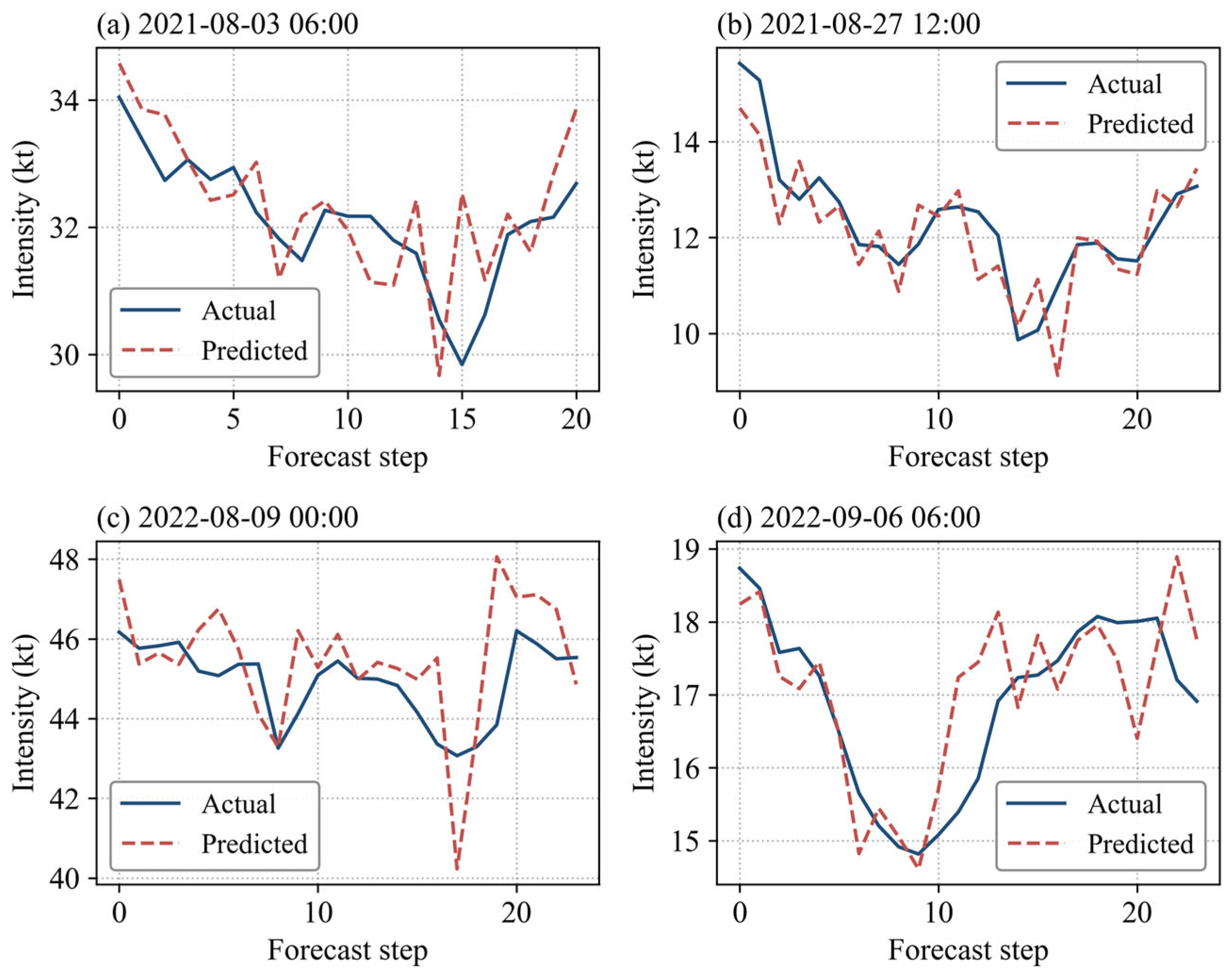
In this section, we present visual analysis of prediction results. As shown in Figure 10, four cases are selected via stratified random sampling stratified by year: two samples are randomly drawn from the 2021 test set and two from the 2022 test set, all with a uniform forecast lead time of 21 h. In this figure, solid blue curves correspond to ground-truth intensity values over the forecast horizon, and dashed red curves denote predictions generated by MADiff. The forecast initialization time is labeled above each subplot. Across all four cases, predicted intensity trajectories closely match the ground truth in terms of overall trend. Non-negligible deviations appear, however, at intensity inflection points and during episodes of rapid intensity fluctuation. This limitation is primarily attributable to the limited temporal resolution of multimodal meteorological inputs, which cannot fully resolve the fine-scale dynamical processes governing rapid TC intensity changes.

6. Conclusions

In this paper, we propose a multimodal-augmented conditional diffusion model (MADiff), the first dedicated framework for waypoint-level TC intensity prediction. By taking multimodal data, including numerical meteorological data, infrared satellite imagery, and TC-related texts, as conditional guidance, MADiff comprehensively characterizes the intensity evolution patterns of TCs at maritime waypoints. The TDConv module captures unified multi-timescale features from multimodal data with inconsistent sampling intervals, eliminating the need for rigid temporal alignment. The DisCF module quantifies cross-modal heterogeneity via information entropy and performs discriminative feature screening, balancing complementary information integration and noise suppression. The Physics-informed regularization term regularizes the diffusion process, further boosting the accuracy of waypoint-level intensity predictions. Across all four Western North Pacific datasets, MADiff achieves average MAE and RMSE values of 2.08 kt and 2.37 kt, outperforming the state-of-the-art baseline by reducing the average MAE by 16.3% and the average RMSE by 10.6%. With approximately 0.40 M trainable parameters and low inference latency, MADiff exhibits promising deployment potential on resource-constrained maritime devices.

Nevertheless, this study still has several limitations. First, the numerical meteorological features and intensity labels used are derived from the ERA5 reanalysis dataset rather than direct in situ observations. Reanalysis data contain inherent systematic uncertainties from numerical assimilation processes, which may affect the absolute accuracy of model training and evaluation. Second, in situ wind observations over open-ocean regions are extremely sparse. The model performance on open-sea waypoints is only verified with reanalysis data, lacking validation from real shipborne or buoy measurements. Third, the model is trained on historical archived datasets with complete quality control. In practical operational scenarios, real-time input data may have latency, missing values and quality fluctuations, leading to potential domain shifts that could degrade prediction performance.

To address these limitations, our future work will focus on four aspects. First, we will collect more buoy and shipborne in situ observation data to construct multi-source benchmark datasets, reduce reliance on reanalysis products, and complete independent performance validation for open-ocean waypoints. Moreover, we will conduct domain adaptation and robustness research for real-time operational data and design targeted adaptation strategies for data latency, missing values and quality fluctuations to narrow the performance gap between historical training and operational deployment. In addition, we will further investigate the key dynamical characteristics across the TC lifecycle and integrate more refined atmospheric dynamic principles as regularization constraints to improve the accuracy and reliability of waypoint-level TC intensity prediction for practical maritime applications. Beyond these methodological improvements, we will also attempt to deploy our method on resource-limited maritime devices to further validate its practical effectiveness.

For practical maritime applications, the model supports two primary use cases. First, for vessel operators and maritime management authorities, MADiff can be embedded within navigation decision support systems, providing quantitative inputs for route risk assessment and voyage planning adjustments. Second, for meteorological technology developers, the modular architecture of MADiff enables flexible reuse and extension. Core components, including TDConv and DisCF, can be directly adapted for other marine meteorological forecasting tasks, and the full framework can be scaled to batch forecasting for large networks of maritime waypoints. For detailed deployment guidance and customized implementation solutions, interested readers may contact the corresponding author.

References

1. Martell-Dubois, R.; Silva-Casarín, R.; Mendoza-Baldwin, E.G.; Muñoz-Pérez, J.J.; Cerdeira-Estrada, S.; Escalante-Mancera, E.; Laiz, I. Spectral bimodality of waves produced by hurricanes in the Caribbean coastal zone off Mexico. Cienc. Mar. 2018, 44, 33–48. [Google Scholar] [CrossRef] [Scilit]
2. Yang, B.; Deng, L.; Xu, N.; Lv, Y.; Cui, Y. Maximum Wave Height Prediction Based on Buoy Data: Application of LightGBM and TCN-BiGRU. J. Mar. Sci. Eng. 2025, 13, 2009. [Google Scholar] [CrossRef] [Scilit]
3. Shi, H.; Song, D.; Yang, G.; Jiang, L.; Wang, X.; He, S. A Three-Stage Deep Learning Framework for Short-Term Tropical Cyclone Track Prediction. J. Mar. Sci. Eng. 2026, 14, 1159. [Google Scholar] [CrossRef] [Scilit]
4. Xiao, Y.; Li, X.; Yao, W.; Chen, J.; Hu, Y. Bidirectional Data-driven Trajectory Prediction for Intelligent Maritime Traffic. IEEE Trans. Intell. Transp. Syst. 2023, 24, 1773–1785. [Google Scholar] [CrossRef] [Scilit]
5. Wang, Y. How Do Outer Spiral Rainbands Affect Tropical Cyclone Structure and Intensity. J. Atmos. Sci. 2009, 66, 1250–1273. [Google Scholar] [CrossRef] [Scilit]
6. Wang, H.; Xu, Q.; Yin, X.; Cheng, Y. Determination of Low-Intensity Tropical Cyclone Centers in Geostationary Satellite Images Using a Physics-Enhanced Deep-Learning Model. IEEE Trans. Geosci. Remote Sens. 2024, 62, 1–10. [Google Scholar] [CrossRef] [Scilit]
7. Wang, F.; Zhang, G.; Yang, D.; Kuang, H. Single-Pass Tropical Cyclone Detector and Scene-Classified Wind Speed Retrieval Model for Spaceborne GNSS Reflectometry. IEEE Trans. Geosci. Remote Sens. 2023, 61, 1–16. [Google Scholar] [CrossRef] [Scilit]
8. Pradhan, R.; Aygun, R.; Maskey, M.; Ramachandran, R.; Cecil, D.J. Tropical Cyclone Intensity Estimation Using a Deep Convolutional Neural Network. IEEE Trans. Image Process. 2018, 27, 692–702. [Google Scholar] [CrossRef] [Scilit] [PubMed]
9. Cho, K.; Merriënboer, B.; Gulcehre, C.; Bahdanau, D.; Bougares, F.; Schwenk, H.; Bengio, Y. Learning Phrase Representations Using RNN Encoder-Decoder for Statistical Machine Translation. In Proceedings of the 2014 Conference on Empirical Methods in Natural Language Processing (EMNLP), Doha, Qatar, 25–29 October 2014; pp. 1724–1734. [Google Scholar]
10. Zhou, H.; Zhang, S.; Peng, J.; Zhang, S.; Li, J.; Xiong, H.; Zhang, W. Informer: Beyond Efficient Transformer for Long Sequence Time-Series Forecasting. In Proceedings of the AAAI Conference on Artificial Intelligence, Online, 2–9 February 2021. [Google Scholar]
11. Neumann, C. An Alternate to the HURRAN (Hurricane Analog) Tropical Cyclone Forecast System; National Weather Service: Silver Spring, MD, USA, 1972; pp. 1–24.
12. DeMaria, M.; Kaplan, J. A Statistical Hurricane Intensity Prediction Scheme (SHIPS) for the Atlantic Basin. Weather Forecast. 1994, 9, 209–220. [Google Scholar] [CrossRef] [Scilit]
13. Chavas, D.; Knaff, J.; Klotzbach, P. A Simple Model for Predicting Tropical Cyclone Minimum Central Pressure from Intensity and Size. Weather Forecast. 2025, 40, 333–346. [Google Scholar] [CrossRef] [Scilit]
14. Alijoyo, F.; Gongada, T.; Kaur, C.; Mageswari, N.; Sekhar, J.; Ramesh, J.V.N.; El-Ebiary, Y.A.; Ulmas, Z. Advanced Hybrid CNN-Bi-LSTM Model Augmented with GA and FFO for Enhanced Cyclone Intensity Forecasting. Alex. Eng. J. 2024, 92, 346–357. [Google Scholar] [CrossRef] [Scilit]
15. Wang, C.; Xiu, Y.; Chen, Z. Cyclone Intensity Prediction via Multispectral Image Sharpening. IEEE Geosci. Remote Sens. Lett. 2024, 21, 1–5. [Google Scholar] [CrossRef] [Scilit]
16. Wu, Y.; Geng, X.; Liu, Z.; Shi, Z. Tropical Cyclone Forecast Using Multitask Deep Learning Framework. IEEE Geosci. Remote Sens. Lett. 2022, 19, 1–5. [Google Scholar] [CrossRef] [Scilit]
17. Tian, W.; Chen, Y.; Song, P.; Xu, H.; Wu, L.; Zhang, Y.; Xiang, C.; Hao, S. TCIP-Net: Quantifying Radial Structure Evolution for Tropical Cyclone Intensity Prediction. IEEE Trans. Geosci. Remote Sens. 2024, 62, 1–14. [Google Scholar] [CrossRef] [Scilit]
18. Wang, X.; Chen, K.; Liu, L.; Han, T.; Li, B.; Bai, L. Global Tropical Cyclone Intensity Forecasting with Multi-Modal Multi-Scale Causal Autoregressive Model. In Proceedings of the IEEE International Conference on Acoustics, Speech and Signal Processing (ICASSP), Hyderabad, India, 6–11 April 2025; pp. 1–5. [Google Scholar]
19. Li, W.; Li, Y.; Yang, Y.; Song, D.; Wei, Z.; Liu, A.-A. Multimodal Adversarial Fusion for Typhoon Intensity Forecasting. IEEE Trans. Geosci. Remote Sens. 2024, 62, 1–12. [Google Scholar] [CrossRef] [Scilit]
20. Wu, H.; Xu, J.; Wang, J.; Long, M. Autoformer: Decomposition Transformers with Auto-Correlation for Long-Term Series Forecasting. In Proceedings of the Annual Conference on Neural Information Processing Systems, Online, 6–14 December 2021. [Google Scholar]
21. Bastami, A.; Aasi, A.; Arghand, H. Estimation of Remaining Useful Life of Rolling Element Bearings Using Wavelet Packet Decomposition and Artificial Neural Network. Iran. J. Sci. Technol. Trans. Electr. Eng. 2019, 43, 233–245. [Google Scholar] [CrossRef] [Scilit]
22. Ho, J.; Jain, A.; Abbeel, P. Denoising Diffusion Probabilistic Models. In Proceedings of the Conference on Neural Information Processing Systems, Online, 6–12 December 2020; pp. 6840–6851. [Google Scholar]
23. Qu, L.; Wang, W.; Li, Y.; Zhang, H.; Nie, L.; Chua, T.-S. Discriminative Probing and Tuning For Text-to-Image Generation. In Proceedings of the IEEE Conference on Computer Vision and Pattern Recognition, Seattle, WA, USA, 16–22 June 2024; pp. 7434–7444. [Google Scholar]
24. Rombach, R.; Blattmann, A.; Lorenz, D.; Esser, P.; Ommer, B. High-Resolution Image Synthesis with Latent Diffusion Models. In Proceedings of the IEEE Conference on Computer Vision and Pattern Recognition, New Orleans, LA, USA, 18–24 June 2022; pp. 10684–10695. [Google Scholar]
25. Ho, J.; Salimans, T.; Gritsenko, A.; Chan, W.; Norouzi, M.; Fleet, D.J. Video Diffusion Models. In Proceedings of the Conference on Neural Information Processing Systems, New Orleans, LA, USA, 28 November–9 December 2022; pp. 1–14. [Google Scholar]
26. Zhu, Y.; Li, Z.; Wang, T.; He, M.; Yao, C. Conditional Text Image Generation with Diffusion Models. In Proceedings of the IEEE Conference on Computer Vision and Pattern Recognition, Vancouver, BC, Canada, 17–24 June 2023; pp. 14235–14253. [Google Scholar]
27. Höllein, L.; Božič, A.; Müller, N.; Novotny, D.; Tseng, H.-Y.; Richardt, C.; Zollhöfer, M.; Nießner, M. ViewDiff: 3D-consistent Image Generation with Text-to-Image Models. In Proceedings of the IEEE Conference on Computer Vision and Pattern Recognition, Seattle, WA, USA, 16–22 June 2024; pp. 5043–5052. [Google Scholar]
28. Hao, F.; Wu, S.; Wei, J.; Zhang, H.; Chua, T.-S. Dysen-VDM: Empowering Dynamics-Aware Text-to-Video Diffusion with LLMs. In Proceedings of the IEEE Conference on Computer Vision and Pattern Recognition, Seattle, WA, USA, 16–22 June 2024; pp. 7641–7653. [Google Scholar]
29. Liu, M.; Huang, H.; Feng, H.; Sun, L.; Du, B.; Fu, Y. PriSTI: A Conditional Diffusion Framework for Spatiotemporal Imputation. In Proceedings of the IEEE 39th International Conference on Data Engineering, Anaheim, CA, USA, 3–7 April 2023; pp. 1927–1939. [Google Scholar]
30. Tashiro, Y.; Song, J.; Song, Y.; Ermon, S. CSDI: Conditional Score-Based Diffusion Models for Probabilistic Time Series Imputation. In Proceedings of the Conference on Neural Information Processing Systems, Online, 6–14 December 2021; pp. 24804–24816. [Google Scholar]
31. Shen, L.; Chen, W.; Kwok, J. Multi-Resolution Diffusion Models for Time Series Forecasting. In Proceedings of the International Conference on Learning Representations (ICLR), Vienna, Austria, 7–11 May 2024. [Google Scholar]
32. Shen, C.; Yu, W.; Zhao, Z.; Song, D.; Cheng, W.; Chen, H.; Ni, J. Multi-modal View Enhanced Large Vision Models for Long-Term Time Series Forecasting. In Proceedings of the Conference on Neural Information Processing Systems, San Diego, CA, USA, 2–7 December 2025. [Google Scholar]
33. Hersbach, H.; Bell, B.; Berrisford, P.; Biavati, G.; Horányi, A.; Muñoz Sabater, J.; Nicolas, J.; Peubey, C.; Radu, R.; Rozum, I.; et al. ERA5 Hourly Data on Single Levels From 1940 to Present. In Copernicus Climate Change Service (C3S) Climate Data Store (CDS); Copernicus Climate Change Service (C3S): Bonn, Germany, 2018. [Google Scholar] [CrossRef]
34. Knapp, K.; Ansari, S.; Bain, C.; Bourassa, M.A.; Dickinson, M.J.; Funk, C.; Helms, C.N.; Hennon, C.C.; Holmes, C.D.; Huffman, G.J.; et al. Globally Gridded Satellite (Gridsat) Observations for Climate Studies. Bull. Am. Meteorol. Soc. 2011, 92, 893–907. [Google Scholar] [CrossRef] [Scilit]
35. Ying, M.; Zhang, W.; Yu, H.; Lu, X.; Feng, J.; Fan, Y.; Zhu, Y.; Chen, D. An Overview of the China Meteorological Administration Tropical Cyclone Database. J. Atmos. Ocean. Technol. 2014, 31, 287–301. [Google Scholar] [CrossRef] [Scilit]
36. Lu, X.; Yu, H.; Ying, M.; Zhao, B.; Zhang, S.; Lin, L.; Bai, L.; Wan, R. Western North Pacific Tropical Cyclone Database Created by the China Meteorological Administration. Adv. Atmos. Sci. 2021, 38, 690–699. [Google Scholar] [CrossRef] [Scilit]
37. Jelesnianski, C. A Numerical Calculation of Storm Tides Induced by A Tropical Storm Impinging on A Continental Shelf. Mon. Weather Rev. 1965, 93, 343–358. [Google Scholar] [CrossRef] [Scilit]
38. Jelesnianski, C.; Chen, J.; Wilson, A. Sea, Lake, and Overland Surges from Hurricanes (SLOSH): Technical Report; National Oceanic and Atmospheric Administration (NOAA): Washington, DC, USA, 1992.
39. Sandler, M.; Howard, A.; Zhu, M.; Zhmoginov, A.; Chen, L. MobileNetV2: Inverted Residuals and Linear Bottlenecks. In Proceedings of the IEEE Conference on Computer Vision and Pattern Recognition (CVPR), Salt Lake City, UT, USA, 18–23 June 2018; pp. 4510–4520. [Google Scholar]
40. Jiao, X.; Yin, Y.; Shang, L.; Jiang, X.; Chen, X.; Li, L.; Wang, F.; Liu, Q. TinyBERT: Distilling BERT for Natural Language Understanding. In Proceedings of the International Conference on Learning Representations (ICLR), Online, 3–7 May 2021. [Google Scholar]
41. Shi, X.; Chen, Z.; Wang, H. Convolutional LSTM Network: A Machine Learning Approach for Precipitation Nowcasting. In Proceedings of the Annual Conference on Neural Information Processing Systems, Montreal, QC, Canada, 7–12 December 2015. [Google Scholar]
42. Hill, D.; McMillan, D.; Bell, K.; Infield, D. Application of Auto-Regressive Models to U.K. Wind Speed Data for Power System Impact Studies. IEEE Trans. Sustain. Energy 2012, 3, 134–141. [Google Scholar] [CrossRef] [Scilit]
43. Rasul, K.; Seward, C.; Schuster, I.; Vollgraf, R. Autoregressive Denoising Diffusion Models for Multivariate Probabilistic Time Series Forecasting. In Proceedings of the International Conference on Learning Representations (ICLR), Online, 3–7 May 2021. [Google Scholar]
44. Shen, L.; Kwok, J.; Zhang, S.; Bai, C. TC-Diffuser: Bi-Condition Multi-Modal Diffusion for Tropical Cyclone Forecasting. In Proceedings of the Thirty-Ninth AAAI Conference on Artificial Intelligence (AAAI), Philadelphia, PA, USA, 25 February–4 March 2025. [Google Scholar]
45. Wang, C.; Li, X.; Zheng, G. Tropical Cyclone Intensity Forecasting Using Model Knowledge Guided Deep Learning Model. Environ. Res. Lett. 2024, 19, 024006. [Google Scholar] [CrossRef] [Scilit]
46. Zhang, X.; Zhuo, J.; Bao, X.; Tan, Z.; Guo, S.; Zhu, K. Integrating Diurnal Pulsing Signatures for AI-Driven Tropical Cyclone Intensity Prediction. Geophys. Res. Lett. 2025, 53, e2025GL119496. [Google Scholar] [CrossRef] [Scilit]
Figure 1. Schematic of center-level and waypoint-level TC intensity prediction. Center-level prediction focuses on the central intensity of the cyclone. Our waypoint-level prediction targets the local wind speed at specific maritime waypoints under TC influence.
Jmse 14 01550 g001
Figure 2. The overall architecture of the proposed MADiff model. Historical multimodal meteorological data are first preprocessed using dedicated encoders and then fed into the TDConv module to extract unified multi-timescale features. The DisCF module then performs discriminative cross-modal fusion at the same timescale and across all timescales to generate comprehensive conditional representations. Finally, fused features are input into the physics-informed conditional diffusion model to produce waypoint-level TC intensity forecasts via reverse denoising.
Jmse 14 01550 g002
Figure 3. The schematic structure of the TDConv module. This module takes unimodal sequential features and corresponding timestamp embeddings as inputs. It generates dynamic convolution parameters via timescale-specific MLP from timestamp embeddings and performs convolution within fixed physical temporal windows. This design adapts to multimodal data with inconsistent sampling intervals and extracts unified multi-timescale features without rigid temporal alignment.
Jmse 14 01550 g003
Figure 4. The schematic structure of the DisCF module. This module consists of two symmetric interaction branches for bidirectional cross-modal information mining. It constructs a comprehensive score matrix by integrating feature similarity and information entropy and implements discriminative feature screening through TopK and BottomK operations to retain both high-correlation complementary features and low-correlation discriminative details. Outputs of the two branches are concatenated to generate the final fusion representation.
Jmse 14 01550 g004
Figure 5. The spatial distribution of all waypoints.
Jmse 14 01550 g005
Figure 6. CRPS compared with different baselines.
Jmse 14 01550 g006
Figure 7. The sensitivity study of key parameters.
Jmse 14 01550 g007
Figure 8. The spatial distribution of waypoints in the Indian and Atlantic Oceans.
Jmse 14 01550 g008
Figure 9. Reliability diagram of uncertainty calibration.
Jmse 14 01550 g009
Figure 10. Visualization of waypoint-level TC intensity prediction for randomly selected samples. Each subplot corresponds to one forecast sample with start time labeled above. The blue curve denotes ground-truth intensity, and the red dashed curve denotes predictions from MADiff.
Jmse 14 01550 g010