Research on Hydrodynamic Performance of a 30 kW Rim-Driven Thruster and Its Coupling Mechanism with an AUV

Abstract

With the continuous expansion of deep-sea resource exploration, marine environmental monitoring, and underwater operations, Autonomous Underwater Vehicles (AUVs) have been increasingly widely applied. Aiming at the demand for high-performance main propulsion systems of Autonomous Underwater Vehicles (AUVs), this paper conducts research on the structural design and hydrodynamic performance of a 30 kW rim-driven thruster (RDT) and its coupling mechanism with AUVs. By combining computational fluid dynamics (CFD) simulations and experimental methods, the influence of the advance coefficient on the open-water performance of the thruster is revealed. An integrated coupling simulation model of the AUV and RDT is established to analyze the performance attenuation law of the thruster and the characteristics of the coupled flow field under wake flow conditions, and to clarify the two-way interaction mechanism between the thruster and AUV. Towing tank tests were carried out at sailing speeds ranging from 1 to 4 kn, which verifies the reliability of the numerical simulation model and the matching performance between the thruster and AUV. The results show that the open-water efficiency of the thruster reaches a peak value of 0.536 at the advance coefficient $\mathrm{J}=0.8$, which is close to the optimal efficiency range with good matching performance of the propulsion system Under wake flow conditions, the attenuation range of the thrust coefficient of the thruster is 12.45–16.53% with the increase in advance coefficient. The main reasons are the uneven inflow velocity and unstable flow field pressure distribution caused by the non-uniform wake flow at the AUV stern. At the ship speeds of 2 kn, 3 kn and 4 kn, the self-propulsion rotational speeds obtained from test fitting are in good agreement with the simulation results, with all relative errors less than 8%. This study provides a theoretical basis and technical reference for the engineering design of medium and high-power rim-driven thrusters as well as the matching optimization of AUV-thruster systems.

1. Introduction

With the continuous expansion of deep-sea resource exploration, marine environmental monitoring, and underwater operations, Autonomous Underwater Vehicles (AUVs) have been increasingly widely applied [1,2]. Higher requirements have been put forward for their sailing speed, endurance, concealment, and reliability [3,4,5]. As the core power unit of an AUV, the main propulsion system directly determines the overall maneuverability and operational efficiency of the vehicle. The traditional shaft-driven propeller adopts a motor-shaft-propeller transmission structure, which suffers from inherent drawbacks, including large transmission losses [6,7] intense vibration and noise, and frequent shaft seal leakage. Hence, it can no longer meet the demands of new-generation AUVs for high power density, low noise, and high reliability [8].

The Rim-Driven Thruster (RDT) is a novel integrated shaftless electric propulsion device [9]. Its rotor and propeller blades are designed as a single unit, while the stator is embedded inside the duct, which completely eliminates the traditional shaft and intermediate transmission components [10,11]. Featuring a compact structure, high propulsion efficiency, low operating noise, and reliable sealing, RDT has become a major development direction for AUV main propulsion systems.

Recent studies on RDTs have mainly focused on the open-water hydrodynamic performance of individual thrusters. Owing to the unique hydraulic structural components of rim-driven thrusters (RDTs), the division of computational domains during simulation modeling is critical to calculation accuracy. Relying on computational fluid dynamics (CFD), Li et al. [12] analyzed the effects of different rotating domain partitioning schemes on the hydrodynamic performance of hub-type rim-driven thrusters. Their study revealed that, for the complex curved walls within the duct region, variations in rotating domain division exert a notable influence on the flow field within the thruster clearance and the spatial distribution characteristics of the wake [13]. Dubas et al. [14] developed a CFD method suitable for steady-state calculations of rim-driven thrusters, and achieved high computational accuracy at low advance coefficients using the SST k-ω turbulence model. Based on the RANS solver, Cao et al. proposed a prediction method for the hydrodynamic performance of rim-driven thrusters and uncovered the distribution law of vortices around propeller blades [15]. Combining the finite element method with CFD techniques, Freeman et al. investigated the hydrodynamic performance of shaftless rim-driven thrusters and verified the potential of this structural layout. The above studies verify that rim-driven thrusters exhibit favorable hydrodynamic performance under single-unit operating conditions [16,17,18].

In terms of ship-engine-propeller coupling research: Newacheck et al. designed a steerable integrated shaftless marine propulsion system and verified its feasibility via ship model tests [19,20]. The Office of Naval Research of the United States, in cooperation with Pacific Marine Supply Company and other institutions, jointly developed megawatt-class rim-driven thrusters (RDTs) [21,22,23]. Mounted on the bow of ships through steel V-shaped struts, this equipment enables vessels to perform rapid turning, emergency collision avoidance, and other maneuvers. Based on the Ka4-70 propeller and Marin 37A duct, Hughes et al. designed and tested a hub-type RDT and analyzed its matching performance with the hull. Taking the dedicated ducted propeller for remotely operated vehicles (ROVs) as the research object [24], Aldias et al. established a complete propeller-duct coupling optimization framework by adopting a technical route integrating parametric modeling, genetic algorithm optimization, and computational fluid dynamics (CFD) simulation verification [25].

The matching performance between RDTs and the hull directly determines the overall propulsive efficiency and maneuverability of marine vessels. Relevant research mainly focuses on three core directions: the flow field mechanism of ship-propeller coupling, layout optimization, and self-propulsion performance verification. A preliminary theoretical and experimental system has been established, which provides crucial support for the practical onboard application of RDTs.

Nevertheless, most existing investigations concentrate on the open-water performance of RDTs under uniform incoming flow, as well as the structural optimization and internal flow evolution of individual thrusters. Research on the coupling mechanism between RDTs and AUV hulls is still insufficient. In practical navigation, the non-uniform wake generated around the AUV stern alters the inflow conditions of the thruster, resulting in considerable changes in its thrust, torque, and efficiency compared with open-water conditions. In addition, most existing studies adopt low-power prototypes (usually below several kilowatts), while numerical simulation and experimental verification for medium-power RDTs (tens of kilowatts) are still limited, which cannot satisfy the engineering requirements of large-tonnage and high-speed AUVs [26].

In view of the above problems, a 30 kW rim-driven thruster matched for a hundred-ton-class AUV is studied in this paper. This study adopts a cylindrical full-flow computational domain and employs the RANS method as well as the SST k-ω turbulence model; a numerical model is established to simulate the open-water performance of the RDT, and the hydrodynamic characteristics under different advance coefficients are analyzed. The reliability of the numerical model is verified by towing tank tests. Furthermore, an integrated coupling simulation model of the AUV and RDT is built to explore the performance degradation and coupled flow field characteristics of the thruster under stern wake conditions [27]. Combined with the comparative analysis of self-propulsion simulation and experimental data, the interaction mechanism between the thruster and AUV hull is revealed.

2. Numerical Simulation on Hydrodynamics of Rim-Driven Thruster

2.1. CFD Numerical Setup for RDT Simulation

Numerical simulations based on the RANS method are carried out to investigate the viscous flow fields of a 30 kW rim-driven thruster under two operating conditions: open water and behind-hull wake. Since the temperature variation in underwater flow is negligible and heat exchange can be ignored, the continuity equation and Reynolds-averaged momentum equations are adopted as the governing equations to resolve complex viscous flow characteristics, including propeller blade rotation, rim gap leakage, and non-uniform stern wake. The complete details of the solver configuration are elaborated as follows.

(1)

Core solver and coupling algorithm

A pressure-based transient solver is selected to solve the viscous flow field. The SIMPLEC algorithm is adopted for pressure–velocity coupling, which provides stable convergence for narrow-rim clearance flow and rotating-blade flow. For spatial discretization, a second-order upwind scheme is applied to the convection terms of momentum, turbulent kinetic energy, and specific dissipation rate; a central differencing scheme is used for all diffusion terms to reduce numerical dissipation.

(2)

Turbulence model and wall treatment

The $SST k\text{-}\omega$ two-equation turbulence model is utilized, which balances the near-wall boundary-layer prediction and far-field wake capture for ducted propulsors. To match the target Y⁺ range of 30–60 on all solid walls, the scalable wall function is activated instead of low-Reynolds wall treatment, avoiding extra mesh refinement inside the viscous sublayer and guaranteeing calculation efficiency.

(3)

Transient sliding mesh settings

The sliding mesh interface is defined between the rotating domain and stationary domain. The rotational speed of the moving zone is assigned according to working conditions, with variable time steps configured to control the blade rotation angle per time step. Three step sizes are tested for uncertainty quantification: $3.47\times {10}^{-3} \mathrm{s}$ ($5°$ per step), $1.39\times {10}^{-3} \mathrm{s}$ ($2°$ per step), $6.94\times {10}^{-3} \mathrm{s}$ ($1°$ per step). For all formal simulations, the time step of $6.94\times {10}^{-3} \mathrm{s}$ is adopted to balance accuracy and computational cost.

(4)

Boundary condition configuration

The far-field inlet boundary is set as a velocity inlet, where axial flow velocity is input according to the target advance coefficient J; initial turbulence intensity is fixed at 5% and turbulent viscosity ratio at 10, consistent with the water tunnel environment. The outlet boundary is defined as a pressure outlet with relative static pressure equal to zero gauge pressure. All surfaces of the blades, rim, and duct are set to no-slip stationary walls, except the rotating region assigned rigid-body rotation motion. Symmetry boundary conditions are applied to the lateral cylindrical faces of the outer computational domain to eliminate far-field boundary interference.

2.2. Numerical Simulation of Rim-Driven Thruster

The research object of this paper is a large, hundred-ton heavy-load autonomous underwater vehicle (AUV), which is mainly applied to long-duration operations in shallow and medium seas, with the capacity to undertake emergency deep-water tasks. Its main body adopts a streamlined revolving hull similar to the SUBOFF standard model. Such a streamlined configuration can effectively reduce frictional resistance and form resistance during navigation. The main propulsion system is mounted at the stern propulsion section of the AUV, providing core power for forward, backward, and depth-keeping cruising motions.

The overall length of the full-scale vehicle model is 36 m, its maximum hull radius is 1.5 m, and its three-dimensional geometric model is shown in Figure 1.

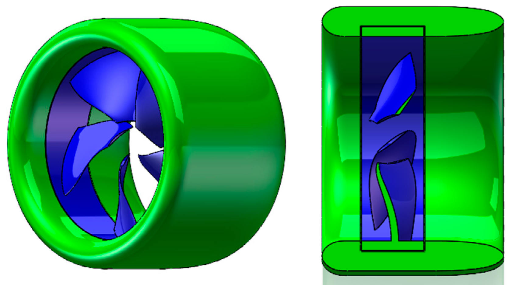
The blade tip of the rim-driven thruster is rigidly connected to the rim while the blade root is free, resulting in the maximum bending moment occurring at the blade tip. Therefore, a reverse thickness distribution design with thick blade tips and thin blade roots is adopted to meet the strength requirements. The main geometric parameters of the thruster are as follows: blade diameter of 800 mm, 5 blades, disk area ratio of 0.7, and duct length of 687.5 mm. The geometric parameters and model of the rim-driven thruster are shown in

Table 1. Main geometric parameters of the thruster.

Item	Unit	Value
Duct length	mm	687.5
Maximum outer diameter of duct	mm	1035
Inner diameter of duct	mm	800
Blade diameter	mm	800
Number of blades	–	5
Disk area ratio	–	0.7
Pitch ratio at 0.7R	–	1.5

and Figure 2.

To calculate the thrust of the designed rim-driven thruster, the design speed of 4 kn $2.0576 \mathrm{m}/\mathrm{s}$, propeller diameter of 0.8 m, fluid density $\mathsf{\rho }=1000 \mathrm{k}\mathrm{g}/{\mathrm{m}}^3$ (fresh water) and design power of 30 kW are adopted as basic parameters. The thrust under ideal inviscid conditions and the actual thrust after viscous correction are calculated, respectively. The detailed calculation procedures and results are presented as follows:

(1)

Thrust Calculation under Ideal Inviscid Conditions

Referring to ducted propellers, the relationship between thrust T and power P for a constant-area ducted propeller is derived based on the momentum theory and energy conservation principle:

$$P={\displaystyle \frac{T}{4}}(3V_{\infty }+\sqrt{V_{\infty }^2+{\displaystyle \frac{4T}{\rho A}}})$$

(1)

where P denotes power, T is thrust, $V_{\infty }$ represents sailing speed, and A is the propeller disk area. Substitute the known parameters into the formula:

$$30000={\displaystyle \frac{T}{4}}(3\times 2.0576+\sqrt{{2.0576}^2+{\displaystyle \frac{4T}{1000\times 0.5027}}})$$

(2)

After simplification:

$$120000=T(6.1728+\sqrt{4.2338+0.007955T})$$

(3)

This is a nonlinear equation requiring numerical solution. Define the function:

$$f\left(T\right)=T(6.1728+\sqrt{4.2338+0.007955T})-120000$$

(4)

The root of $f\left(T\right)=0$ is solved, and the final thrust is obtained as $T=8256 \mathrm{N}$. Verification is conducted by substituting the result back into the formula:

$$P_{cal}={\displaystyle \frac{8256}{4}}\times (6.1728+8.3612)\approx 30000$$

(5)

(2)

Viscous Correction

The actual thrust is corrected from the ideal value via the overall propulsion efficiency:

$$T_{actual}=T_{ideal}\cdot \eta$$

(6)

where $\eta$ denotes the overall propulsion efficiency, which consists of two components:

Hydraulic efficiency ${\mathsf{\eta }}_{\mathrm{h}}$: accounts for losses caused by fluid viscosity, including friction, vortex flow, and flow separation;

Mechanical efficiency ${\mathsf{\eta }}_{\mathrm{m}}$: accounts for losses induced by mechanical motion such as friction and vibration.

The hydraulic efficiency is determined by the thrust loading coefficient ${\mathrm{C}}_{\mathrm{T}}:$

$$C_T={\displaystyle \frac{T}{\frac{1}{2}\rho V_{\infty }^2}}$$

(7)

Substituting the target thrust $T=8256 \mathrm{N} \mathrm{y}\mathrm{i}\mathrm{e}\mathrm{l}\mathrm{d}\mathrm{s} C_T=7.76,$ which corresponds to a medium loading condition. According to marine propulsion experience, the typical hydraulic efficiency range of ducted rim-driven thrusters under this load coefficient is 0.75 to 0.85.

Adopting representative characteristic values, where the mechanical efficiency ${\eta }_m=0.97$ and hydraulic efficiency ${\eta }_h=0.85$, the overall propulsion efficiency is calculated as 0.8245. The actual thrust is expressed as

$${\mathrm{T}}_{\mathrm{a}\mathrm{c}\mathrm{t}\mathrm{u}\mathrm{a}\mathrm{l}}=0.8245\times 8256 \mathrm{N}=6807 \mathrm{N}$$

(8)

Therefore, the propeller with a diameter of $800 \mathrm{m}\mathrm{m}$ can generate a thrust of 6807 N at the sailing speed of 4 kn.

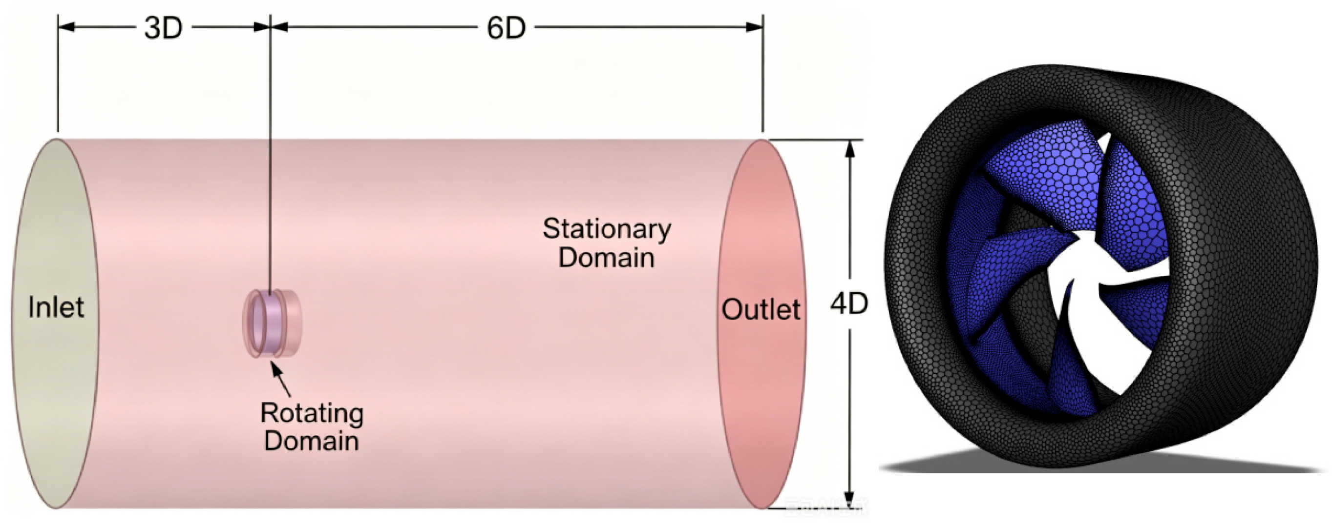
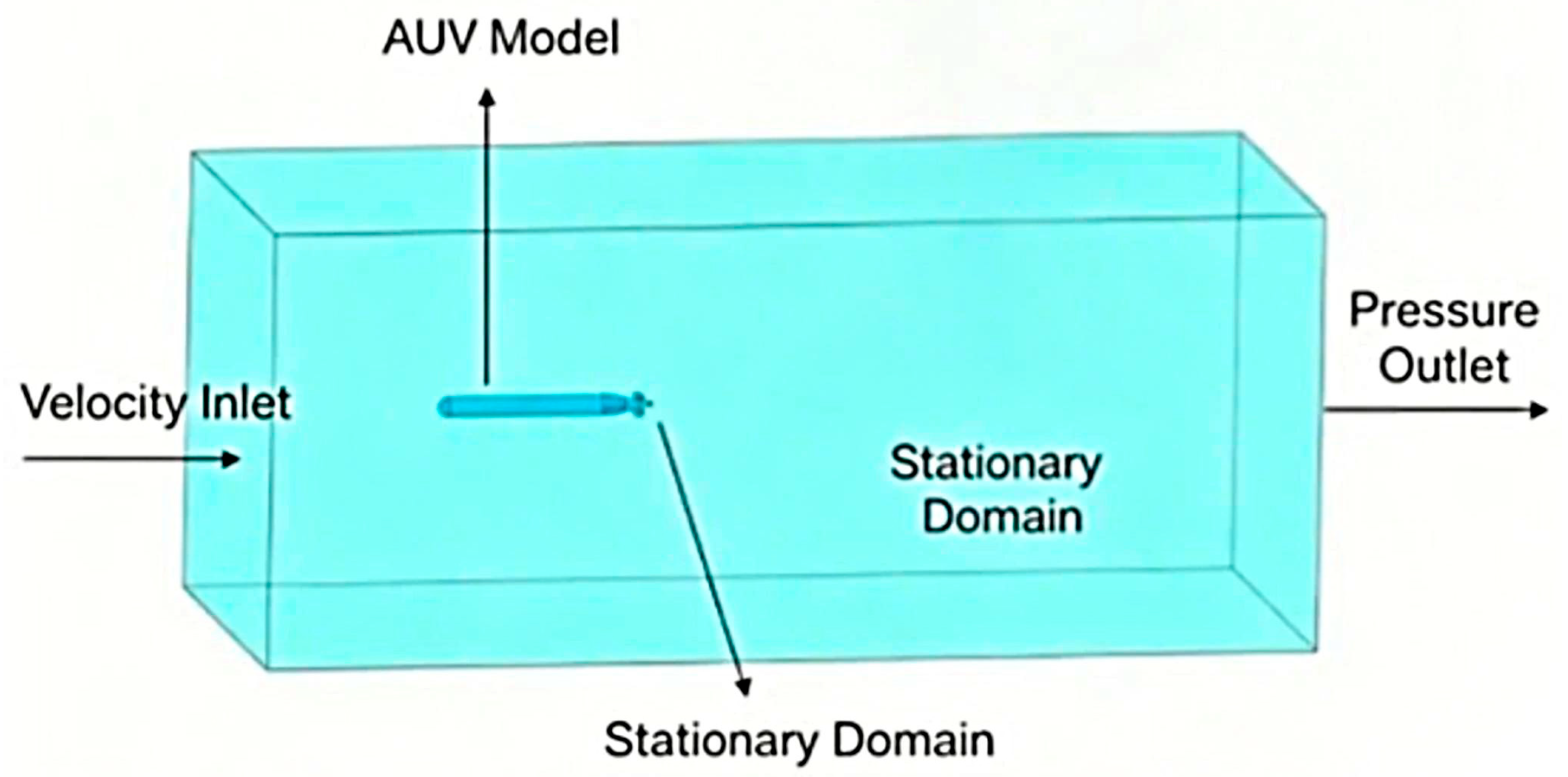
A cylindrical full-flow computational domain is adopted for simulation, which is divided into a rotating domain and a stationary domain. The diameter of the stationary domain is 4D, with an inlet length of 3D and an outlet length of 6D (D refers to the blade diameter). The diameter of the rotating domain is 2 mm larger than the outer diameter of the rim. For the complex curved walls within the duct region and propeller rotating domain, to accurately resolve the near-wall flow characteristics, the dimensionless wall distance Y⁺ is controlled within the range of 30–60 for all solid walls. This target range is deliberately selected in accordance with the standard practice for wall-function-based simulations. In the present study, the scalable wall function is employed in conjunction with the $SST k\text{-}\omega$ turbulence model. This Y⁺ range ensures that the first near-wall cell lies safely within the log-law region, where the wall function is theoretically valid, while avoiding the buffer layer (5 < Y⁺ < 30) and the viscous sublayer (Y⁺ < 5), where the standard wall function would lose accuracy.

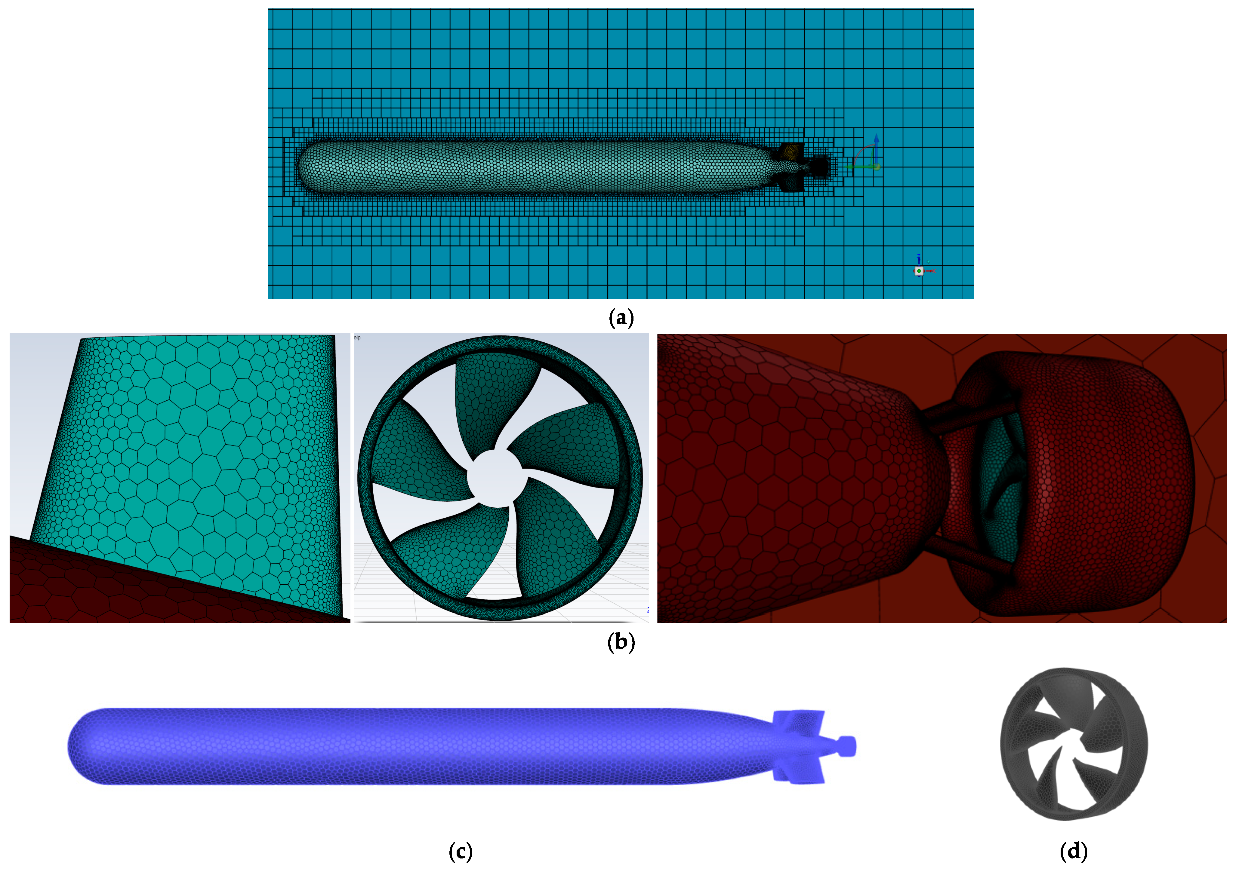
To accurately capture critical flow details, including pressure gradients, flow field variations, and tip clearance vortices within the gap, local mesh refinement is implemented for the clearance region with a refined mesh size of 0.05 mm. The first layer thickness of the boundary layer inflation adjacent to the blade and hub surfaces in the rotating domain is set to 0.01 mm, with a total of 15 inflation layers generated. Given the narrow clearance between the propeller blades and the duct, the maximum gap dimension is specified as 0.1 mm, and the mesh size on the blade surfaces is limited to 1 mm. The Reynolds-Averaged Navier–Stokes (RANS) method and SST $\mathrm{k}\text{-}\mathsf{\omega }$ turbulence model are employed. The inlet is set as a velocity inlet and the outlet as a pressure outlet. The walls of the propeller and duct are defined as no-slip walls, and the rotating domain adopts a rotating coordinate system. The computational domain and surface mesh of the rim-driven thruster are illustrated in Figure 3.

In CFD numerical simulations, mesh quality and cell count directly govern the solution accuracy of flow fields, while exerting notable impacts on computational efficiency and convergence performance. To eliminate the interference of mesh density on numerical results and balance simulation precision with computational efficiency, six sets of computational cases with total mesh cells increasing gradually from 1 million to 8 million are designed in this study for grid independence verification. The advance coefficient $J=0.6$ and rotational speed of 240 rpm are selected as the validation conditions, with thrust coefficient $K_T$ adopted as the primary evaluation indicator. The mesh cell numbers corresponding to each case are listed in

Table 2. Mesh cell counts for different computational cases.

Case Number	Total Mesh Cells/104
Case 1	100
Case 2	200
Case 3	400
Case 4	520
Case 5	680
Case 6	800

.

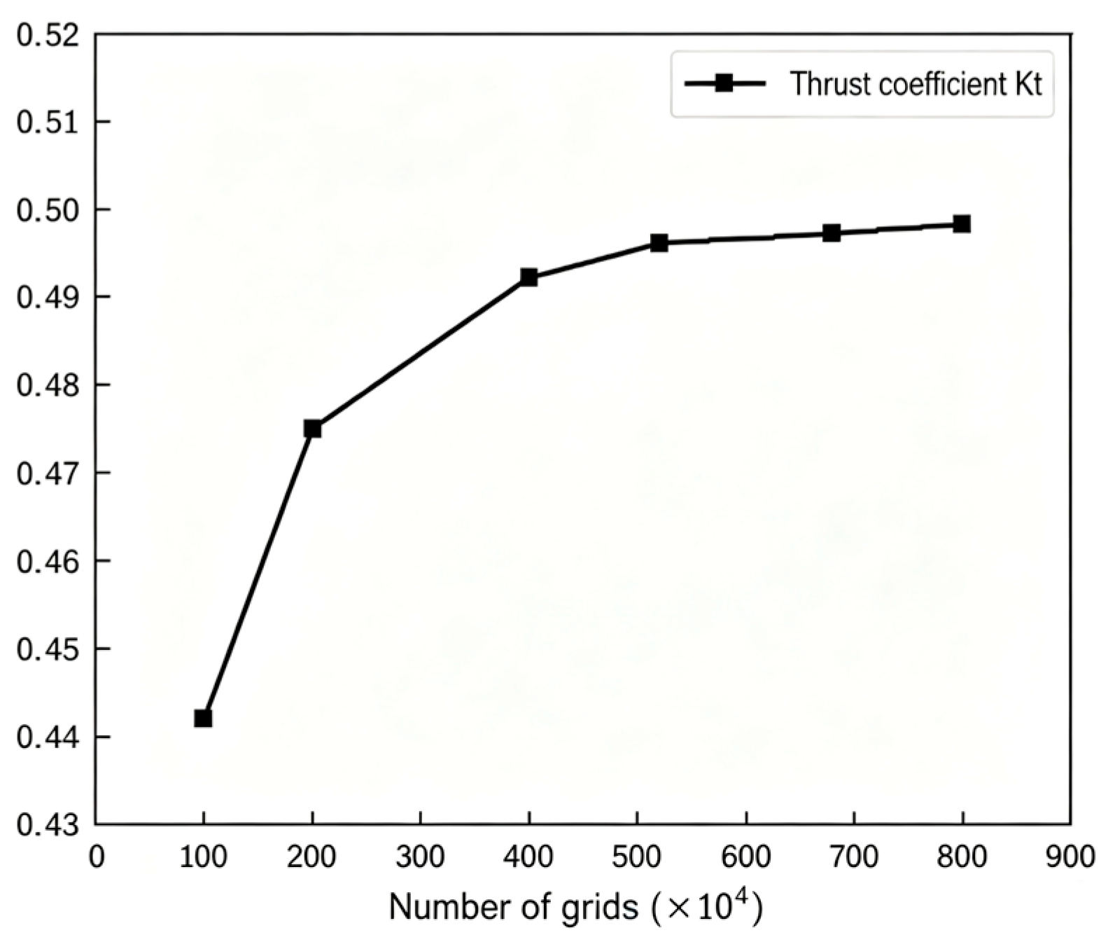
With all other computational conditions maintained identical, numerical simulations are conducted on six rim-driven thruster models with distinct mesh cell counts. The calculated thrust coefficients and corresponding relative errors under each mesh scheme are acquired, and the computational results for various mesh quantities are illustrated in Figure 4.

As indicated by the grid independence verification results, the numerical predictions gradually converge without obvious fluctuations once the total mesh cell count exceeds 5.2 million. This demonstrates that adopting a mesh size of approximately 5.2 million cells for subsequent calculations can effectively reduce hardware resource consumption and computational costs while guaranteeing numerical accuracy. Accordingly, all follow-up numerical simulations of the rim-driven thruster model are performed with mesh quantities ranging from 5.2 million to 6.8 million cells.

To systematically investigate the open-water performance of the rim-driven thruster, the rotational speed is set to 240 rpm, and the advance coefficient is adjusted by changing the axial incoming flow velocity. The open-water performance results of the thruster at the advance coefficient $\mathrm{J}=0.2\sim 0.8$ are listed in

Table 3. Simulation results of open-water performance of the rim-driven thruster.

Advance Coefficient J	Thrust Coefficient KT	Torque Coefficient 10 KQ	Open-Water Efficiency η0
0.2	0.7755	1.009	0.2447
0.3	0.6922	0.986	0.3352
0.4	0.6139	0.952	0.4104
0.5	0.5354	0.917	0.4645
0.6	0.4610	0.868	0.5073
0.7	0.3877	0.813	0.5314
0.8	0.3151	0.748	0.5360

.

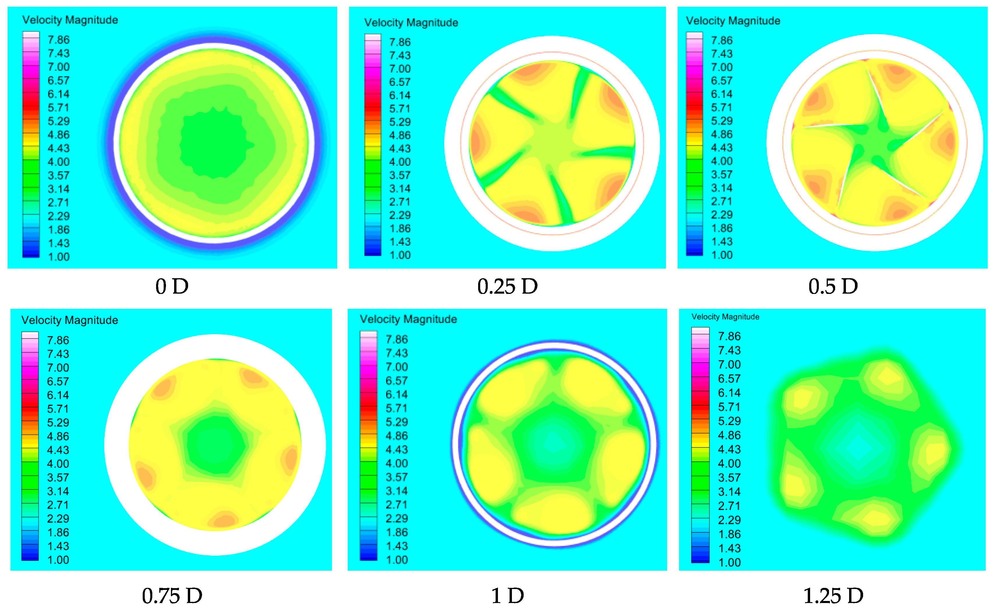
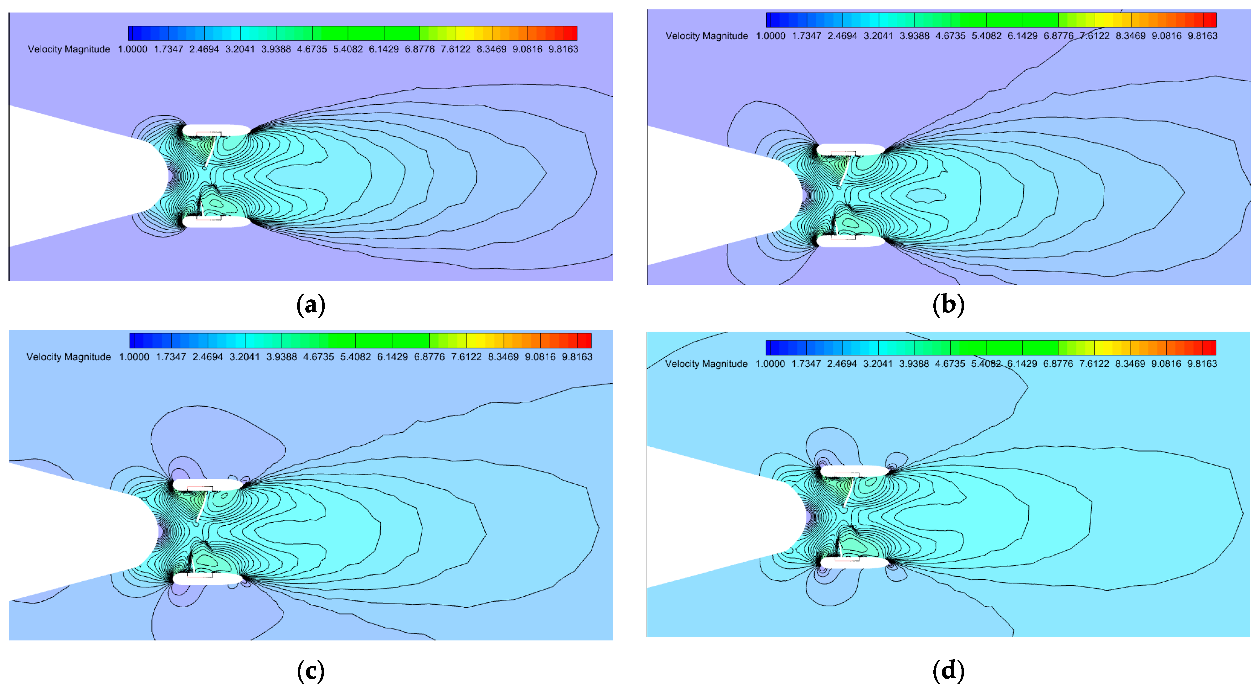
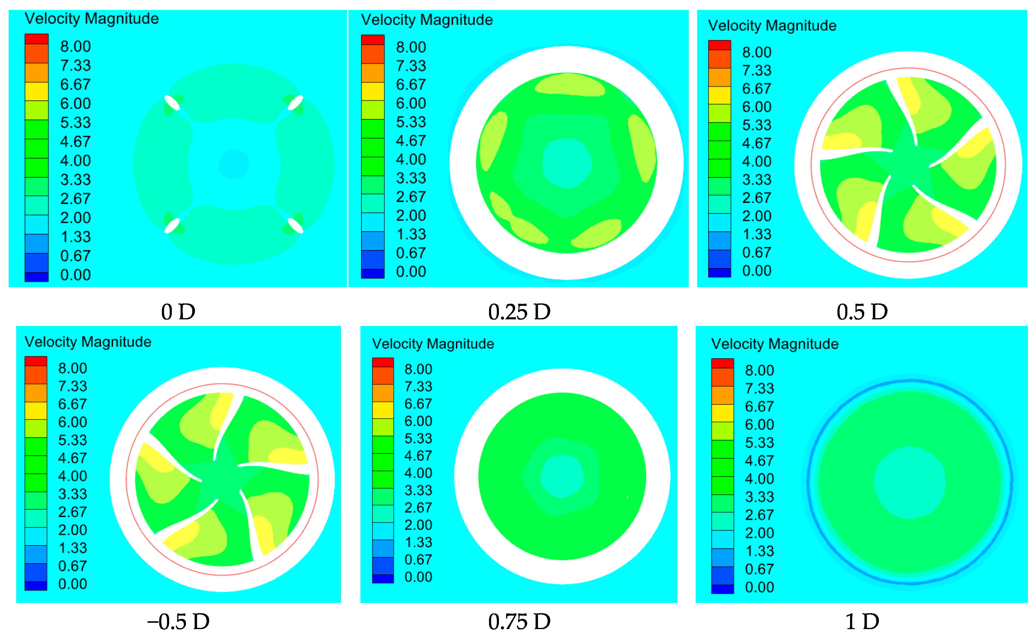
Taking the inlet section of the thruster (0 D) as the starting point and defining the flow direction at the outlet as the positive axial direction, the velocity distributions at six characteristic axial sections of 0 D, 0.25 D, 0.5 D, 0.75 D, 1 D, and 1.25 D are extracted to analyze the axial evolution characteristics of the flow field. The contour plots of different sections are shown in Figure 5.

In terms of the axial evolution of the flow field, the incoming flow remains uniform in the upstream region of the thruster (0 D~−0.55 D). A slight rise in flow velocity occurs near the duct inlet, which reflects the suction effect of the rim-driven thruster. At the propeller disk (0.5 D), the flow field is disturbed by rotating blades, resulting in obvious circumferential non-uniformity of velocity distribution, where the high-velocity regions correspond exactly to the positions of the blades. In the downstream area of the rim-driven thruster (0.75 D~1 D), the swirling flow generated by blade rotation gradually diffuses, and the flow velocity decreases along the axial direction until the flow field returns to a uniform state. The intensity of swirling flow at sections downstream of 0.5 D decays by more than 40%. The flow field basically restores an axisymmetric distribution at the sections of 1 D and 1.25 D.

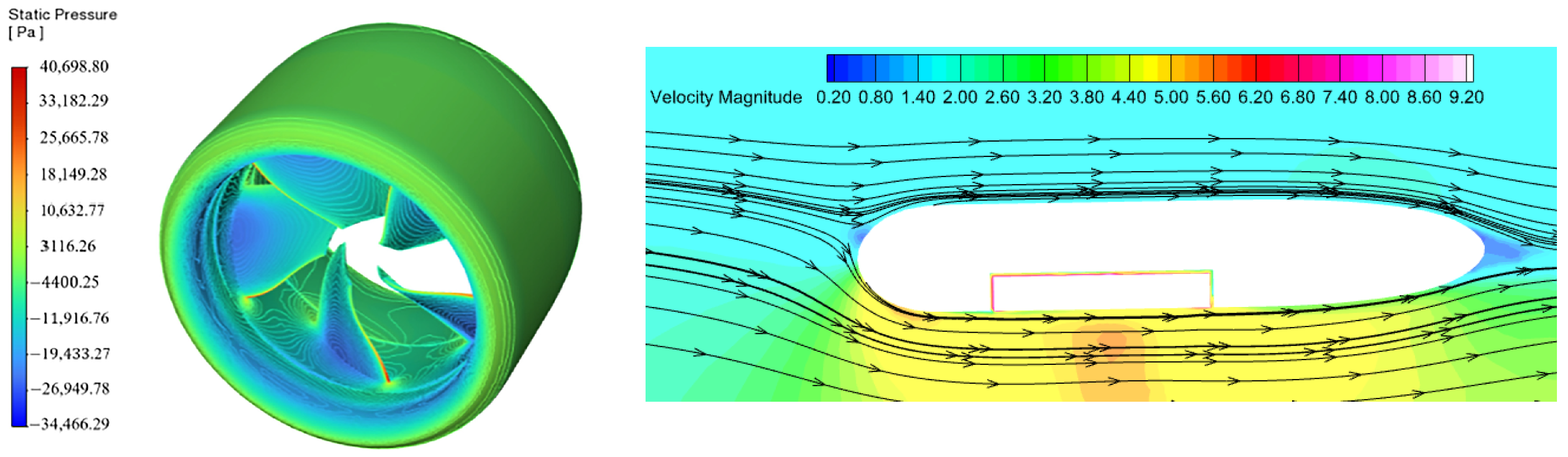
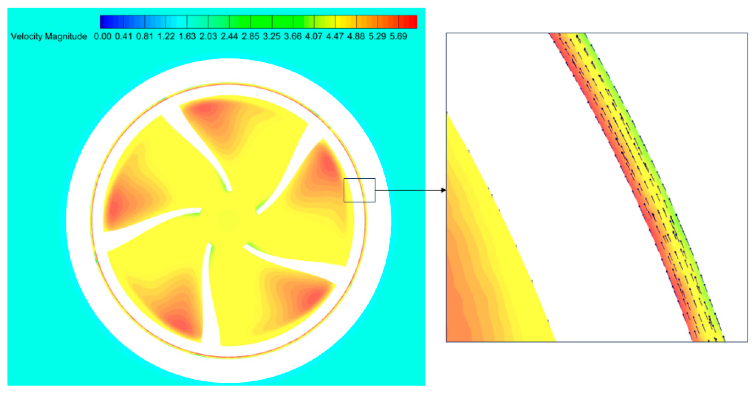
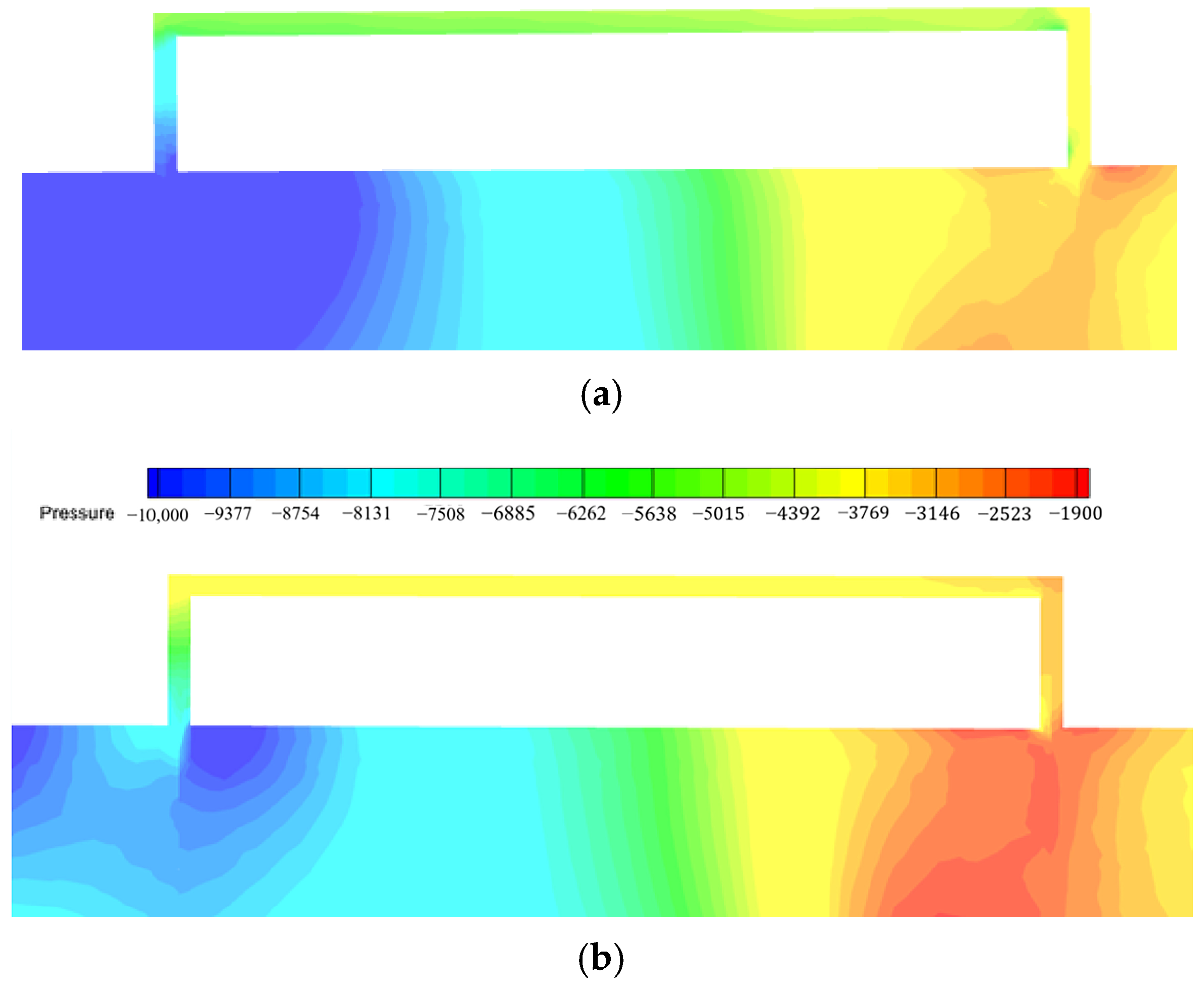
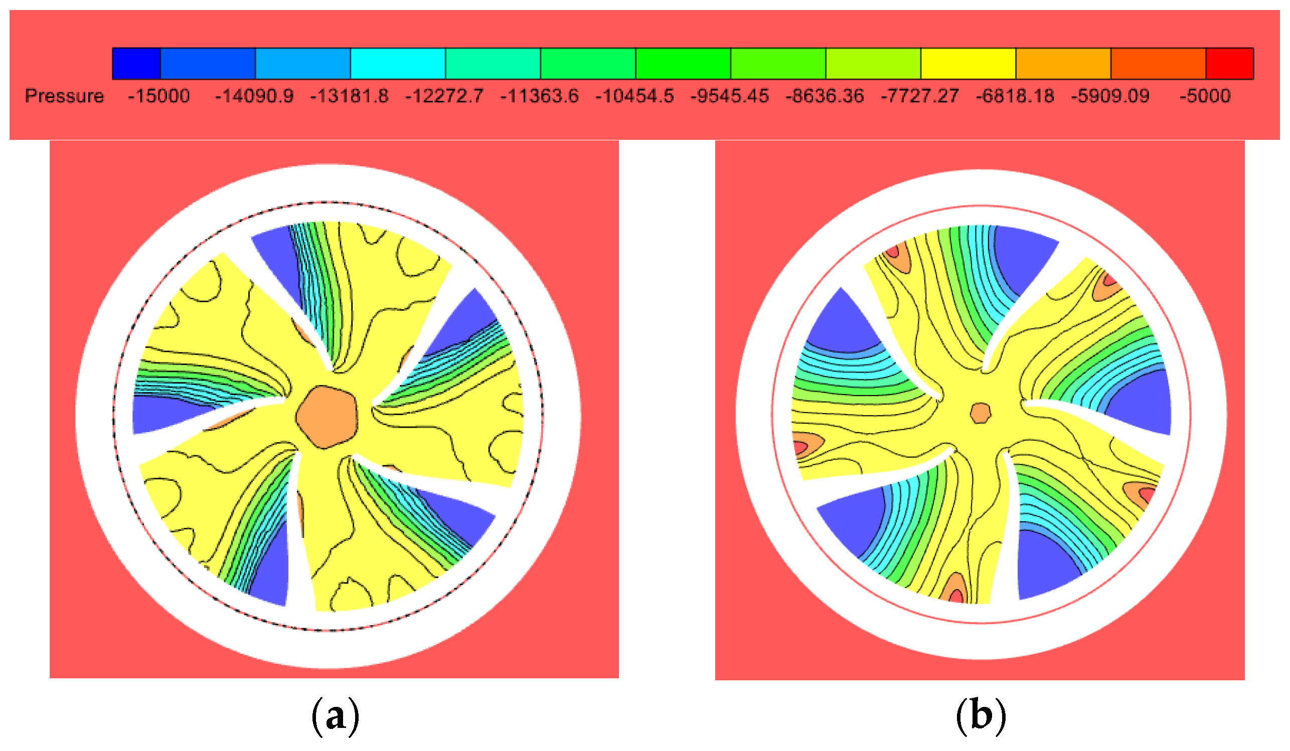
According to the simulation results for axial velocity contours (Figure 6) and global pressure and flow field contours (Figure 6), the pressure on the outer wall of the duct is distributed uniformly and is roughly equal to the ambient pressure of the incoming flow. Pressure variation is mainly concentrated inside the duct passage. Divided by the propeller disk, the interior of the duct presents a distinct three-stage pressure distribution: the area ahead of the propeller disk is a low-pressure zone, the middle throat section serves as a medium-pressure transition zone, and the area behind the propeller disk is a high-pressure zone. The axial pressure difference between the inlet and outlet of the duct produces positive thrust on the duct itself, indicating that the duct can achieve an obvious thrust-augmentation effect under heavy-load and low advance-coefficient conditions.

2.3. CFD Uncertainty Quantification Analysis

The CFD uncertainty quantification analysis in this paper covers three independent components: grid discretization uncertainty, temporal discretization uncertainty, and iterative convergence uncertainty. A full set of uncertainty quantification analyses is carried out for the benchmark open-water condition of the single thruster with advance coefficient (J = 0.6) and rotational speed (n = 240 rpm). The calculation of grid discretization uncertainty in this study strictly complies with the ITTC standard for CFD verification. Meanwhile, the systematic procedure proposed by Eça for estimating numerical uncertainties of CFD computations via grid refinement studies is also adopted [28,29].

2.3.1. Mesh Discretization Uncertainty Quantification

(1)

Mesh Scheme Design

Three sets of unstructured meshes with identical topology and systematic uniform refinement are adopted. Only the mesh size is changed proportionally, while all other boundary conditions, discretization schemes, and turbulence models remain exactly the same. The basic mesh parameters are listed in

Table 4. Basic mesh parameters.

Mesh Level	Total Cell Count	Height of the First Near-Wall Cell	Controlled Range of Y+	Refinement Ratio r
Coarse Mesh	200	0.02 mm	40–70	-
Medium Mesh	400	0.015 mm	35–55	1.26
Fine Mesh	800	0.01 mm	30–45	1.26

.

(2)

Computational method

Based on Richardson extrapolation theory, the actual convergence order p is first solved using the target physical quantity (thrust coefficient $K_T$) obtained from the three sets of meshes, and then the Grid Convergence Index (GCI) of the fine mesh is calculated. The formulas are given as follows:

Convergence Order Calculation:

$$p={\displaystyle \frac{ln\left(\frac{f_1-f_2}{f_2-f_3}\right)}{\ln r}}$$

where $f_1,f_2,f_3$ are the target physical quantities under coarse, medium, and fine meshes, respectively; r denotes the mesh refinement ratio.

Grid Convergence Index (GCI):

$${GCI}_{fine}=F_s·{\displaystyle \frac{\left|\frac{f_1-f_2}{f_{3.}}\right|}{r^p-1}}$$

where $F_s$ represents the safety factor, which takes a standard value of 1.25 for three mesh sets; ${GCI}_{fine}$ denotes the relative mesh discretization uncertainty $U_{grid}$ of the fine mesh.

(3)

Quantification Results

The thrust coefficients calculated from the three mesh sets are: $f_1=0.4750$, $f_2=0.4660$, $f_3=0.4588$. Substituting these values into the formulas yields:

The actual convergence order is approximately $p\approx 0.97$, which falls within the monotonic asymptotic convergence range and conforms to the law of numerical convergence.

The Grid Convergence Index of the fine mesh is ${GCI}_{fine}=2.12\%$, meaning the mesh discretization uncertainty $U_{grid}=2.12\%$.

This result indicates that for the computational meshes of 5.20 million~6.80 million cells adopted in this work, the discretization error falls within the engineering-acceptable range (the generally accepted industry threshold is less than 3%), and the mesh resolution satisfies the requirement for computational accuracy.

The computational domain of the AUV-thruster coupled system includes the complete AUV hull, X-shaped rudders, and thruster. The total mesh count is approximately three times that of the single-thruster model, which brings a considerable rise in transient computational cost. Limited by computational resources, the full three-mesh GCI analysis was not repeated for the coupled system. However, the coupled system adopts exactly the same mesh-generation strategy, boundary-layer growth ratio, local refinement criteria, and Y⁺ control range as the single-thruster model throughout the simulation. Convergence has been verified via mesh-refinement comparisons in key regions. Consequently, its mesh discretization uncertainty is the same order of magnitude as that of the single-thruster model, laying a consistent foundation for the reliability of numerical results.

2.3.2. Temporal Discretization Uncertainty Quantification

A transient sliding-mesh approach is adopted in this paper to simulate the rotation of propeller blades. The discretization error induced by time-step size constitutes an essential component of numerical uncertainty, and its quantification method shares the same origin as the mesh-based GCI.

(1)

Time Step Scheme

Three sets of proportionally scaled time-step sizes are selected. The corresponding propeller blade rotation angles per time step are $5°$, $2°$, and $1°$. At a rotational speed of 240 rpm, the corresponding time-step sizes are $3.47\times {10}^{-3} \mathrm{s}$, $1.39\times {10}^{-3}\mathrm{s}$, and $6.94\times {10}^{-4}\mathrm{s}$, respectively. All other computational settings remain identical.

(2)

Quantification Results

Adopting the same calculation method as the mesh-based GCI, the time-step convergence order $p_t\approx 1.15$ is obtained, and the temporal convergence index for the fine time-step ${\mathrm{G}\mathrm{C}\mathrm{I}}_{\mathrm{t}}\approx 0.87\mathrm{\%}$, namely, the temporal discretization uncertainty ${\mathrm{U}}_{\mathrm{t}\mathrm{i}\mathrm{m}\mathrm{e}}=0.87\mathrm{\%}$.

The results demonstrate that the time-step setup adopted in this work is sufficiently convergent. The temporal discretization error is very small and contributes little to the overall numerical uncertainty.

2.3.3. Iterative Convergence Uncertainty Quantification

Iteration error refers to the fluctuation error induced by iterative solving within each time step, which is quantified by a statistical method in this work:

1. After the computation is fully converged, the thrust coefficient is continuously monitored over 20 complete propeller-blade rotation cycles, and sample data in the steady-state segment are extracted.

2. The relative standard deviation within the 95% confidence interval is taken as the iterative uncertainty:

$${\mathrm{U}}_{\mathrm{i}\mathrm{t}\mathrm{e}\mathrm{r}}={\displaystyle \frac{2s}{\overline{f}}}\times 100\%$$

where S denotes the sample standard deviation, and $\overline{f}$ represents the mean value of the physical quantity.

The calculated relative iterative-convergence uncertainty under the baseline condition is ${\mathrm{U}}_{\mathrm{i}\mathrm{t}\mathrm{e}\mathrm{r}}\approx 0.32\%$. This indicates that the dual convergence criteria for residuals and physical quantities are reasonably set, and the iteration error can be neglected.

2.3.4. Synthesis of Total Numerical Uncertainty

The three types of errors, i.e., mesh discretization error, temporal discretization error, and iterative convergence error, are mutually independent. The root-sum-square method is adopted to synthesize the total numerical uncertainty:

$${\mathrm{U}}_{\mathrm{n}\mathrm{u}\mathrm{m}}=\sqrt{U_{grid}^2+U_{time}^2+U_{iter}^2}$$

Substituting each component for calculation yields that the total relative numerical uncertainty ${\mathrm{U}}_{\mathrm{n}\mathrm{u}\mathrm{m}}\approx 2.31\%$ under the baseline condition. The overall result achieves a relatively high-accuracy level and satisfies the engineering accuracy requirements for CFD numerical prediction of marine propulsors.

3. Tank Towing Test

Tank towing tests are conducted to verify the actual hydrodynamic performance of the 30 kW rim-driven thruster and check the reliability of the numerical simulation model.

The main dimensions of the towing tank are 120 m in length, 8 m in width, and 4 m in depth, with a constant water depth of 4 m. The water temperature during tests is maintained within the range of 15.5–25.5 °C. The tank is equipped with an all-electric towing carriage with a maximum design speed of 5 m/s and a velocity control accuracy of ±0.001 m/s, which enables accurate simulation of the designed cruising speed of the AUV ranging from 1 kn to 4 kn. The parallelism error of the carriage rails is no greater than 0.1 mm/m, guaranteeing stable and disturbance-free towing conditions. Regular waves (period: 0.4–4.0 s, wave height: 0.05–0.4 m) and irregular waves (ITTC spectrum, ISSC spectrum, significant wave height: 0.05–0.32 m) can be generated to reproduce complex marine environmental conditions. The test facility is illustrated in Figure 7 and Figure 8.

Figure 8. Physical photograph of the 30 kW rim-driven thruster.

Figure 8. Physical photograph of the 30 kW rim-driven thruster.

The main contents of the test are as follows: the carriage travels at a speed ranging from 1 kn to 4 kn. The frequency converter is adjusted to output speed signals to start the rim-driven thruster and drive the rotor to rotate in water. The thruster operates at different rotational speeds starting from 0 rpm, and parameters such as rated thrust and power are recorded when each working condition runs stably.

The specific test procedures are described below:

(1)

The calibrated rim-driven thruster is mounted at the stern of the full-scale fairing model, and positioning tooling is used to ensure the alignment accuracy between the thruster axis and the model axis.

(2)

Control the carriage to move at a constant preset speed. After the carriage speed, thruster rotational speed, and thrust value all become stable, collect parameters including thrust, rotational speed, and input power synchronously via the data acquisition system.

(3)

Keep the sailing speed unchanged, and increase the rotational speed of the thruster step by step at an increment of 30 rpm to complete the tests of all rotational speed conditions under the current speed.

(4)

Adjust the carriage speed to 1 kn, 2 kn, 3 kn and 4 kn in sequence, and repeat Steps (2) and (3) to finish all tests.

According to the experimental data, the rotational speed-thrust characteristic curves at different sailing speeds are plotted, as shown in Figure 9.

It can be observed that the thrust of the rim-driven thruster increases nonlinearly with rotational speed at all speeds, which approximately conform to the hydrodynamic law that thrust is proportional to the square of rotational speed, matching the design expectation. To further verify the reliability of the numerical simulation method, simulation results are compared with towing test data under different rotational speeds at 1 kn and 4 kn (see Figure 10).

The comparison results show that the thrust obtained by simulation is in good agreement with test data at low speed, with a relative error of 0.75~10.81%. The error is less than 3% at medium and high rotational speeds (120~180 rpm), which verifies the reliability of the numerical simulation model under uniform inflow conditions.

At high speed (4 kn), except for the low rotational speed critical region, the relative error ranges from 10.92% to 22.92%, which is higher than that at low speed. The main reasons are as follows: the non-uniformity of the wake flow at the AUV stern is enhanced at high speed, leading to more complex flow-field disturbance in the test; the simplified treatment of wake flow in the simulation model causes deviations. In addition, the assembly gap between the thruster and the fairing, as well as profile transition deviation in the test, induces local flow separation. Meanwhile, the flow field of the thruster installed behind the fairing in the test differs from the actual wake flow of AUVs.

4. Simulation on Coupling Performance of Rim-Driven Thruster and AUV

4.1. Analysis of Hydrodynamic Performance Under Wake Flow Conditions

For the flow field characteristics of the coupled system consisting of an AUV and a rim-driven thruster, a cuboid full-flow computational domain is established. The computational domain is divided into two subdomains: a stationary domain and a rotating domain. The stationary domain covers the entire AUV and far-field flow region, while the rotating domain fully encloses the propeller blades and rim rotor of the rim-driven thruster. Flow field data exchange between the two subdomains is realized via the Interface boundary.

All peripheral surfaces of the computational domain are defined as symmetry boundaries to construct a numerical towing tank. The specific dimensional settings are as follows: the distance from the inlet boundary to the AUV bow is 2L, and the distance from the outlet boundary to the AUV stern is 3L (where L denotes the overall length of the AUV). The vertical and lateral boundaries are all spaced 2L away from the AUV surface. Such dimensions can fully contain the flow around the AUV hull and the wake induced by the thruster, eliminating the interference of far-field boundaries on numerical results. The computational domain model is presented in Figure 11.

Hexahedron-dominated meshes are adopted for discretization, with local refinement on the AUV surface, X-shaped rudders, thruster blades, and gaps. The growth rate of boundary layer meshes is set to 1.2 to meet the requirements of turbulence-model calculations (see Figure 12).

By varying the effective inflow velocity, corrected from the AUV speed with wake effects, the thrust and torque of the thruster at different advance coefficients under the wake field behind the AUV hull are calculated. The hydrodynamic results under wake conditions are listed in

Table 5. Hydrodynamic results of the rim-driven thruster under wake flow conditions.

Advance Coefficient J	Thrust Coefficient KT	Torque Coefficient 10 KQ	Efficiency η
0.2	0.679	0.992	0.218
0.3	0.614	0.968	0.303
0.4	0.544	0.933	0.371
0.5	0.476	0.886	0.427
0.6	0.409	0.837	0.466
0.7	0.338	0.779	0.486
0.8	0.263	0.712	0.471

.

The hydrodynamic calculation results of the rim-driven thruster under wake flow conditions in Table 5 are compared with its open-water data, and the comparison is presented in Figure 13.

The hydrodynamic data under wake flow conditions are compared with the open-water data of the thruster (see Figure 13). It is found that the variation rules of hydrodynamic performance of the stern-mounted thruster with advance coefficient are consistent with those under open-water conditions: the thrust coefficient and torque coefficient decrease gradually with the increase in flow velocity, while the efficiency rises first and then drops. Compared with open-water conditions, the thrust coefficient, torque coefficient, and efficiency of the thruster all decrease obviously under stern wake flow, and the attenuation degree increases with the rise in advance coefficient. When $\mathrm{J}=0.2$, the thrust coefficient decreases by about 12.45%; when $\mathrm{J}=0.8$, the attenuation amplitude reaches 16.53%.

4.2. Self-Propulsion Simulation

Based on the self-propulsion analysis method, this section carries out self-propulsion numerical simulations within the designed speed range to solve the self-propulsion equilibrium points at various sailing speeds and quantify the power-matching characteristics between the propulsion system and the AUV.

The mesh generation scheme, computational domain setup, and boundary condition configurations adopted in the simulations remain consistent with those described in Section 4.1. The rotational speed of the rim-driven thruster inside the rotating subdomain is adjusted to balance the thrust generated by the thruster against the total resistance of the AUV, whereby the self-propulsion points corresponding to different sailing speeds are determined.

After obtaining the characteristic curves of rotational speed versus thrust, the curves are combined with the resistance data of the AUV. The Origin 2025 software is utilized to plot curves with rotational speed on the horizontal axis and thrust/resistance on the vertical axis. The coordinate values of the intersection points of the two curves are extracted via the built-in analysis tools of the software. Combined with interpolation and iterative solving algorithms, the simulated thrust values at various rotational speeds within the sailing speed range of 1–4 kn are acquired, as presented in Figure 14.

The self-propulsion equilibrium points at different speeds are calculated and listed in

Table 6. Calculation results of self-propulsion equilibrium points for AUV-rim-driven thruster system.

Speed (kn)	Speed (m/s)	Calculated Self-Propulsion Speed (rpm)	Calculated Thrust at Self-Propulsion Point (N)
1.0	0.514	61.31	292.75
2.0	1.028	135.1	1111.19
3.0	1.542	199.8	2510.46
4.0	2.056	284.8	4564.51

.

The self-propulsion analysis results show that the equilibrium rotational speed increases approximately linearly with the rise in sailing speed. From 1 kn to 4 kn, the rotational speed increases by about 4.6 times, which is basically consistent with the trend that resistance increases with the square of speed. The self-propulsion results prove that the 30 kW rim-driven thruster matches well with the target AUV within the full speed range, and the designed thruster has stable thrust response characteristics under all sailing conditions.

Combined with the navigation resistance data of the target AUV at speeds of 1–4 kn, the towing test results are fitted to obtain the self-propulsion equilibrium points of the rim-driven thruster at different sailing speeds. The obtained results are then compared with the self-propulsion rotational speeds calculated by coupled simulation, as shown in

Table 7. Comparison of self-propulsion points between towing tests.

Speed	Test Self-Propulsion Speed (rpm)	Simulated Self-Propulsion Speed (rpm)	Relative Deviation (%)
1 kn	48	61.31	21.7
2 kn	136	135.1	0.67
3 kn	197	199.8	1.40
4 kn	264	284.8	7.30

.

To intuitively demonstrate the differences and variation trends between the self-propulsion speeds obtained from experimental fitting and coupled simulation at different sailing speeds, the data in Table 6 are plotted into comparison curves, as shown in Figure 15.

The results show that both the fitted and numerically calculated self-propulsion speeds increase in an approximately linear manner. At speeds of 2 kn, 3 kn, and 4 kn, the fitted speeds agree well with the simulation results, with all relative errors below 8%. The relative error reaches 21.7% at the low speed of 1 kn. This is mainly because the flow field in the towing tank is vulnerable to minor disturbances and low-range measurement errors under low-speed conditions. Meanwhile, the total resistance of the AUV is small at this speed, making the equilibrium point between thrust and resistance highly sensitive to measurement errors. Overall, the findings verify that the adopted coupled simulation method can accurately predict the self-propulsion matching performance of the AUV and rim-driven thruster. The obtained self-propulsion equilibrium points can provide a reliable reference for determining the actual operating conditions of the AUV main propulsion system.

4.3. Analysis of Characteristics of Coupled Flow Field and Pressure Field

To reveal the internal flow mechanism of performance variation in the thruster under wake flow conditions, the flow field differences between the operating and non-operating states of the thruster at 240 rpm under 4 kn are compared (see Figure 16).

An obvious velocity gradient zone is formed in the transition area from the bow to the parallel section due to profile variation. Compared with open-water conditions, the upstream flow field of the stern-mounted thruster is affected by the surrounding flow of the AUV stern, featuring an evident velocity gradient and uneven inflow velocity. This leads to different hydrodynamic loads at different circumferential positions of the propeller disk, which is a major cause of increased torque coefficient. The accelerated flow at the AUV stern has little influence on the boundary layer state of the front and middle parts of the AUV.

The wake diffusion degree increases with the rise in sailing speed, evolving from axisymmetric contraction at 1 kn to asymmetric diffusion at 3 kn. The intensified wake diffusion causes the effective thrust generated by the thruster to diffuse to the surrounding flow field and reduces the thrust transmission efficiency (see Figure 17).

Taking the inlet of the rim-driven thruster as the reference, the velocity distributions at six axial characteristic sections including 0 D, −0.25 D, 0 D, 0.25 D, 0.5 D and 1 D are extracted toward the outlet to analyze the axial evolution characteristics of the flow field. The corresponding contour plots are presented in Figure 18.

The flow characteristics are analyzed based on the velocity contours. At the upstream sections of 0 D and 0.5 D, the flow field suffers obvious velocity distortion due to the hull wake and non-uniform incoming flow behind the AUV stern. The incoming flow no longer maintains a uniform state, and the circumferential velocity difference across the sections increases significantly. At the core sections where the blades are located $0.5 D \mathrm{a}\mathrm{n}\mathrm{d}-0.5 D$ velocity variation is highly concentrated around the blades and the gaps of the rim structure. High-velocity regions appear on the working surfaces of the blades and within the rim gaps. As the fluid flows downstream away from the rim-driven blades, the driving effect of the blades gradually weakens at the subsequent sections of 0.5 D, 0.75 D, and 1 D. The diffusion path of blade trailing vortices deviates, the velocity gradient becomes gentle, the flow turbulence is remarkably reduced, and the flow velocity declines at a lower rate.

To further explore the flow evolution characteristics inside the gap, the velocity and pressure fields in the rotor ring gap are analyzed. The axial velocity distribution of the flow field in the rotor ring gap is shown in Figure 19, and the longitudinal section pressure distribution of the rotor ring is presented in Figure 20a.

It can be observed that after the fluid enters the rotor gap, it gradually deflects in the circumferential direction under the inertial effect of the rotor ring, accompanied by a decrease in axial velocity. This explains the occurrence of velocity peaks on the right-side wall in Figure 19. Restricted by the geometric configuration of the rotor-ring gap, flow separation takes place when the fluid passes through the corners of the flow passage, and local vortices form near the wall, resulting in substantial local energy loss. Combined with the local high pressure at each corner, an annular main flow is generated inside the passage, which further intensifies the non-uniformity of the flow field.

Comparing the gap pressure distributions at different incoming flow velocities in Figure 20, it is found that the local high-pressure area at the gap inlet shrinks as the incoming flow velocity increases, while the opposite trend appears at the gap outlet. At the sailing speed of 4 kn, an obvious pressure boundary forms between the blade surface and the surrounding flow field. Compared with the condition at 1 kn, the pressure difference between the blade face and blade back decreases remarkably, which directly leads to a reduction in the thrust output of the rim-driven thruster. Based on the above analysis of velocity and pressure fields, the flow within the gap is highly complex and unstable. Flow separation at the gap inlet, vortex structures inside the gap, and backflow at the gap outlet are the typical characteristics of gap leakage flow. Such flow not only directly consumes the effective energy of the thruster, but also disturbs the main flow field, thereby indirectly reducing the overall efficiency of the thruster.

Further comparative analysis of the flow-field pressure distribution of the thruster under open-water conditions and AUV stern-mounting conditions is carried out to explore the hydrodynamic performance differences between the uniform ideal flow field and the actual stern wake flow field (see Figure 21).

There are remarkable differences in pressure distribution between the open-water flow field and the AUV stern flow field. Under open-water conditions, the pressure distribution around the rim-driven thruster is uniform and axisymmetric. The pressure variation rule on the blades is clear: the leading edge is a high-pressure area, and the trailing edge is a low-pressure area, with pressure transitioning steadily from the leading edge to the trailing edge. The overall pressure of the propeller disk remains at a high level, which creates favorable flow conditions for thrust output. Under stern wake flow conditions, the flow field of the thruster is directly affected by the non-uniform wake flow at the AUV stern and presents an obvious left-right asymmetry. The high-pressure area on the right side of the thruster is larger, with a more significant pressure gradient.

4.4. Limitations

Despite the valuable findings obtained in this study, several limitations should be acknowledged that constrain the scope and generalizability of the results.

(1) The numerical simulations are based on the RANS equations combined with the SST k-ω turbulence model, which inherently adopts the Reynolds-averaging approach. While this method captures time-averaged flow characteristics effectively, it may not fully resolve intricate unsteady flow phenomena within the rim gap and detailed vortex structures in the stern wake region. The unsteady interaction between the rotating blades and the non-uniform wake flow, as well as the transient pressure fluctuations on the blade surfaces, could be underestimated by the steady-state simulation framework adopted in this work.

(2) The investigated speed range is limited to 1–4 kn, which primarily covers the low-to-medium cruising conditions of the AUV. The hydrodynamic performance and coupling characteristics at higher sailing speeds, where the wake flow becomes more complex and the boundary-layer separation may intensify, remain unexplored. Additionally, only the straight-ahead navigation condition is considered; maneuvering conditions such as turning, diving, and ascending, which involve significantly different inflow angles and wake distributions, are not included in the current analysis.

(3) The self-propulsion simulation employs a quasi-steady approach by matching the thrust and resistance curves, rather than performing a fully coupled dynamic self-propulsion calculation. This simplification may overlook transient mutual feedback between AUV motion and thruster performance during actual navigation. Furthermore, the fluid–structure interaction (FSI) effects, including structural deformation of the blades and rim under hydrodynamic loads, are not incorporated in the present simulations, which could affect the accuracy of performance prediction, especially under high-load operating conditions.

5. Conclusions

Combined with the structural characteristics of the rim-driven thruster and the simulation requirements for rotating machinery, this paper adopts a cylindrical full-flow computational domain, which is divided into two parts: a rotating inner domain and a stationary outer domain. The RANS equations and SST k-ω turbulence model are employed for numerical calculations, and the sliding mesh technique is applied at the interface between the stationary domain and the propeller rotating domain of the rim-driven thruster. This paper establishes an integrated coupling simulation model of an AUV and a 30 kW rim-driven thruster for a hundred-ton-class AUV. Comparative analyses on open-water performance, performance under wake flow conditions, and self-propulsion matching characteristics are conducted, and the main conclusions are drawn as follows:

(1)

The towing tank tests verify the actual hydrodynamic performance of the thruster. The thrust increases nonlinearly with rotational speed and approximately follows the square law. The open-water efficiency reaches a peak of 0.536 at the advance coefficient $\mathrm{J}=0.8$, which is well matched with the cruising condition of the AUV.

(2)

The coupling interaction mechanism between the AUV and rim-driven thruster is clarified. The hydrodynamic performance of the thruster degrades obviously under wake-flow conditions. The attenuation range of the thrust coefficient is 12.45~16.53% with the increase in advance coefficient. The fundamental reasons are the uneven inflow velocity and unstable pressure distribution of the flow field induced by the non-uniform wake flow at the AUV stern.

(3)

At speeds of 2 kn, 3 kn and 4 kn, the fitted speeds agree well with the simulation results, with all relative errors below 8%, which verifies the reliability of the established numerical model. The thrust data show good agreement. This research provides a theoretical basis and technical reference for the operating condition setting of AUV main propulsion systems and for the engineering design of medium- and high-power rim-driven thrusters.

This paper systematically investigates the design, numerical simulation, and experimental tests of a 30 kW rim-driven thruster (RDT), and some research achievements have been obtained. Nevertheless, several limitations remain to be further explored in future work: the investigation of the cavitation performance of rim-driven thrusters. The effects of cavitation on thruster performance are not fully considered in the numerical simulations and experimental tests of this work. Under operating conditions of high rotational speed and low advance coefficient, cavitation easily occurs on the suction side of propeller blades, which deteriorates thrust output and induces vibration and noise. Further numerical simulations and experimental research on RDT cavitation performance will be carried out to reveal the evolution law of cavitation and provide support for cavitation suppression design.