ODARRL: Obstacle- and Disturbance-Aware End-to-End Residual Reinforcement Learning for Underwater Robot Trajectory Tracking with Obstacle Avoidance

Abstract

ROVs are essential for marine exploration and underwater operations, yet conventional teleoperation relies heavily on skilled human operators, and many autonomous methods stop at high-level planning rather than low-level actuation, limiting robustness in disturbed and cluttered environments. This paper proposes ODARRL, an obstacle- and disturbance-aware sensor-to-thruster (ST) end-to-end residual reinforcement learning framework for safe trajectory execution of underwater robots. Using a three-stage curriculum, ODARRL first acquires a basic policy from MPC demonstrations in a static obstacle-free environment, then improves disturbance-robust tracking under random currents, and finally extends to scenarios involving both currents and obstacles. A Dual-Horizon Attention Disturbance Encoder is further designed to capture current-related features from long- and short-term histories, which are fused with robot states and reference information as the input to the ST end-to-end policy. Experiments in Marine Gym with BlueROV2 Heavy demonstrate that ODARRL achieves more stable and robust trajectory tracking under random currents, reducing the mean total tracking error by 69.3%, 31.9%, 45.8%, 73.0% and 25.8% relative to the MPC-imitation policy, PPO, SAC, A2C and VNRS-SAC, respectively. With obstacles introduced, curriculum-initialized policies also exhibit higher path progress and more stable task completion during obstacle-avoidance training.

1. Introduction

Underwater robots play a critical role in modern ocean exploration and underwater operations. In recent years, increasing investment in ocean exploration and exploitation has further emphasized the importance of underwater robotic systems. Among these systems, remotely operated vehicles (ROVs) have become indispensable platforms because they enable operations in environments that are inaccessible or highly challenging for divers, and they support tasks that are difficult to complete manually, including deep-sea resource exploration, equipment maintenance, and aquaculture support [1,2,3].

Despite these advantages, the operation of ROVs still depends heavily on experienced human operators. Long-duration missions impose a considerable workload on operators and may reduce both the safety and efficiency of task execution. Therefore, improving the autonomy of ROVs has become an important objective. Previous studies have introduced a range of classical control methods into underwater robot control, including PID [4], MPC [5], and SMC [6]. Although these methods are effective in specific scenarios, they usually rely on strong prior assumptions about the system structure or model accuracy [7].

To improve robustness against nonlinear dynamics and environmental disturbances, many control methods introduce artificial neural networks [8,9,10,11]. Compared with purely classical methods, these approaches provide stronger adaptability to complex dynamics and uncertain environments. However, most existing methods still depend on manually designed control structures or nominal models, and their performance is sensitive to the distribution of training data and the selection of network hyperparameters. As a result, limitations in sample efficiency, stability, and generalization remain evident in complex underwater tasks [12].

In response to these challenges, machine learning methods have attracted growing attention, with imitation learning (IL) and reinforcement learning (RL) forming two major technical directions. IL has achieved strong results in quadruped robots [13], humanoid robots [14], and aerial robots [15] because of its training efficiency and reduced sensitivity to hyperparameters [13]. However, since IL essentially learns from expert datasets, the performance of the learned policy is often bounded by the quality and coverage of the demonstrations [16]. In addition, as discussed above, the difficulty of obtaining expert datasets is a major bottleneck for IL [13]. This issue is particularly severe for underwater robots and partly explains why IL-based studies remain limited in this field. By contrast, RL has been widely used in various robotic domains because of its strong optimization capability [17], and deep RL has shown the potential to exceed human experts in certain robotic tasks [18]. Deep RL has also been widely applied to underwater robots [19,20,21]. Nevertheless, it usually requires extensive simulation before convergence. The problems of sparse rewards and high exploration cost become especially pronounced when the controller directly acts at the low-level execution layer [12].

To balance training efficiency and final policy performance, a common strategy is to initialize a policy with prior data and then refine it through RL [22,23]. Related efforts have also emerged in underwater robotics. For example, Zhang et al. [24] propose VNRS-SAC, a reward-shaping-based soft actor–critic method for random trajectory tracking of AUVs. This method uses expert data for policy pretraining and potential-based reward shaping to strengthen the initial reward signal and alleviate sparse rewards during the early stage of training. Other studies learn a reward predictor from human expert preferences to provide an improved reward signal [25]. Although these expert-data-based methods can mitigate sparse rewards during early training, they still face the practical difficulty of collecting human expert data in underwater environments. Lyu et al. [26] avoid the use of human expert data by adopting a hierarchical structure that separates the perception-to-planning process from the planning-to-execution process, and they introduce hindsight experience replay (HER) to alleviate sparse rewards. However, this strategy is limited to off-policy learning. Another important limitation of many existing underwater robot control studies is that controller validation often still relies on simplified numerical simulations. In such settings, underwater robots are commonly abstracted as point masses, planar vehicles, or low-dimensional dynamical systems, while the execution-layer constraints of real ROVs are not explicitly considered. These simplifications facilitate algorithm development and rapid testing, but they may ignore key physical factors such as thrust allocation constraints, actuator saturation, nonlinear hydrodynamic coupling, and restoring forces. Consequently, policies developed under such settings may face substantial difficulties when deployed on real robotic platforms.

Beyond these issues, the complexity and uncertainty of ocean environments introduce additional challenges for policy learning [27]. To address this problem, previous studies have explored different methods for perceiving flow fields or reducing the influence of ocean currents on control performance. Specifically, Gao et al. [28] introduce learnable Fourier features that map the state into a learnable Fourier basis space, and they initialize the variance of the Fourier basis so that the Q-network first captures low-frequency signals while filtering high-frequency noise. However, this method focuses more on extracting noise-resistant information than on perceiving the specific influence of currents on the robot. Gunnarson et al. [29] directly measure surrounding flow velocity by adding extra sensors, but this approach increases system cost. Yao et al. [30] and Chu et al. [31] adopt teacher-student frameworks to learn latent representations of flow fields. However, this paradigm relies on privileged information during training, and the performance of the student network is affected by teacher quality and distillation error. In particular, Yao et al. [30] focus on flow-field adaptation for amphibious quadruped propulsion without considering obstacle avoidance. To address the above problems, this paper proposes ODARRL, an obstacle- and disturbance-aware residual reinforcement learning framework for underwater robot trajectory tracking with obstacle avoidance. The main contributions of this paper are summarized as follows:

• This paper develops an end-to-end trajectory tracking controller under full six-degree-of-freedom dynamics, actuator dynamics, and practical control constraints. By reducing the gap between theoretical validation and practical execution caused by the simplified numerical models widely used in existing studies, the proposed setting improves the physical fidelity of the learned policy and its potential for real-world application.
• This paper proposes a three-stage curriculum learning framework with policy initialization guided by non-human expert data. In this framework, MPC-guided imitation learning provides a feasible initial policy, while reinforcement learning further improves the initialized policy beyond expert demonstrations. This design greatly reduces the difficulty of obtaining expert datasets, improves the feasibility of data collection, and enhances training efficiency and stability.
• This paper designs a Dual-Horizon Attention Disturbance Encoder (DADE) to learn control-relevant disturbance representations from long-horizon and short-horizon observation histories. This module improves disturbance-aware decision making without explicitly estimating flow-field variables.

All experiments are conducted in Marine Gym [32] using the BlueROV2 Heavy platform. The experimental results show that ODARRL outperforms classical control methods and general RL baselines. In the trajectory tracking task under ocean current disturbances, ODARRL reduces the mean tracking error by 69.3%, 31.9%, 45.8%, 73.0% and 25.8% compared with MPC-imitation policy, PPO, SAC, A2C and VNRS-SAC, respectively. In environments with both currents and obstacles, the proposed method achieves stronger path-progress capability and a more stable learning process than other initialization strategies, which further demonstrates the effectiveness of the three-stage curriculum learning framework.

The rest of this paper is organized as follows. Section 2 formulates the ROV trajectory tracking problem in environments with ocean currents and obstacles. Section 3 introduces the proposed staged reinforcement learning algorithm, ODARRL. Section 4 presents the Marine Gym simulation platform, the training procedure, the experimental results, and the corresponding discussion. Finally, Section 5 concludes this paper and discusses future work.

2. Background

2.1. Mathematical Model of ROV

In this work, simulations are conducted using BlueROV2 Heavy (Blue Robotics, Torrance, CA, USA). BlueROV2 Heavy is a highly extensible remotely operated vehicle (ROV) with an open-frame structure that can accommodate a wide range of electronic devices, battery packs, thrusters, buoyancy foam, and payloads. This simple and robust design makes it convenient to install additional modules, such as stereo cameras, forward-looking sonar, and a DVL. BlueROV2 Heavy has a length of 457 mm, a width of 575 mm, a height of 254 mm, and a weight of 11 kg. It can operate at depths greater than 100 m, reach a maximum cruising speed of 3 knots, and support an endurance of approximately 3 h. BlueROV2 Heavy is equipped with eight thrusters. Four thrusters are used for horizontal motion control, while the remaining thrusters support vertical motion and attitude regulation. Through these thrusters, BlueROV2 Heavy can generate up to 9 kgf of forward and lateral thrust and up to 14 kgf of vertical thrust. With multiple onboard sensors, BlueROV2 Heavy is capable of performing various tasks, including automatic heading regulation, path tracking, and path planning.

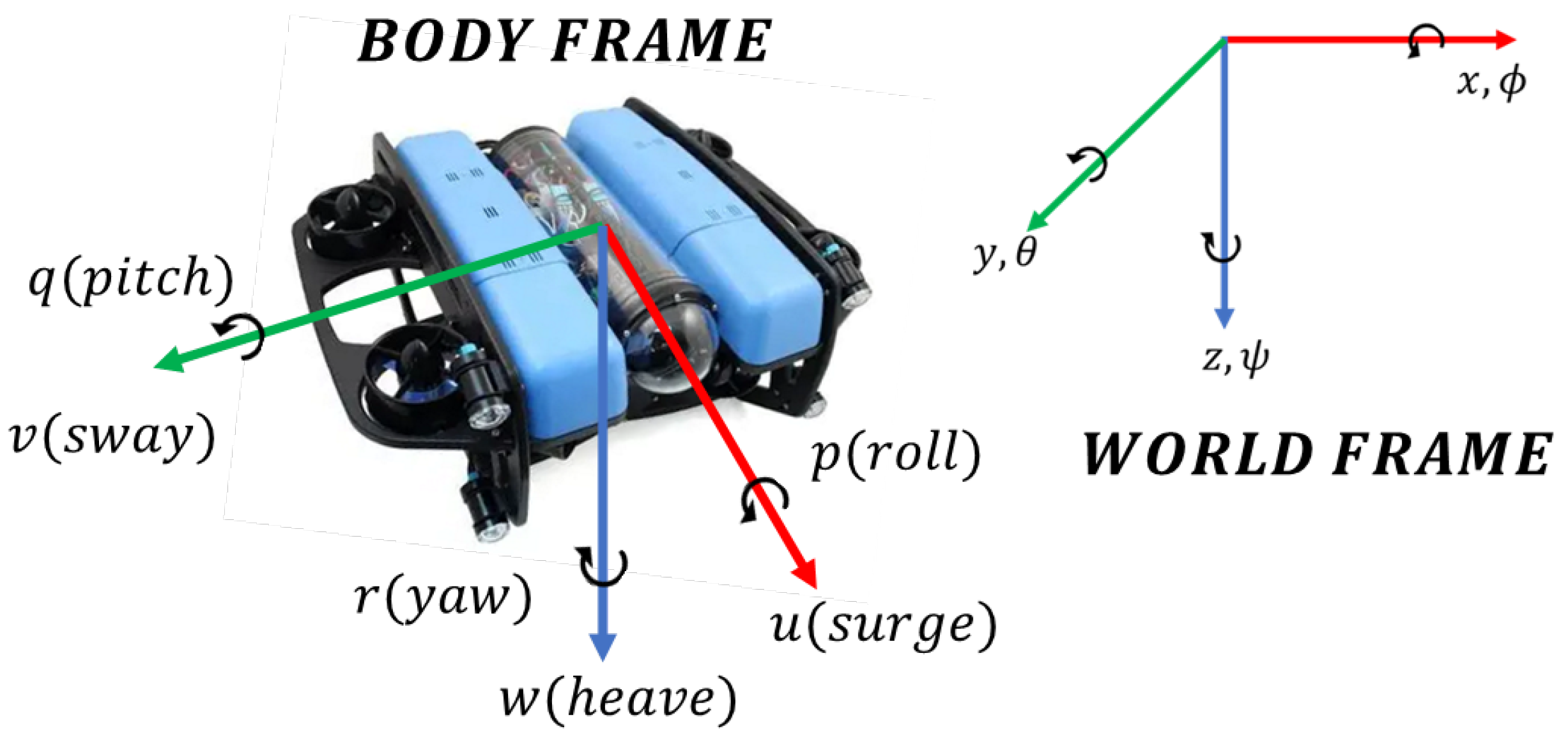
BlueROV2 Heavy has six degrees of freedom. The definitions of the body frame and the world frame are illustrated in Figure 1. In this work, the dynamic representation of Fossen [33] is adopted, and the kinematic model of the vehicle is described as

$$\dot{\eta }=J\left(\eta \right)\nu ,$$

(1)

where $\dot{\eta }$ denotes the time derivative of the position and attitude vector, and

$$\eta ={\left[\begin{array}{cccccc}x& y& z& \varphi & \theta & \psi \end{array}\right]}^T,$$

(2)

which represents the position and Euler angles with respect to the world coordinate system. The vector $\nu$ denotes the body-frame velocity, and $J\left(\eta \right)$ is the Jacobian matrix that maps the body-frame velocity to the time derivatives of position and attitude. More specifically,

$$\dot{\eta }={\left[\begin{array}{cccccc}\dot{x}& \dot{y}& \dot{z}& \dot{\varphi }& \dot{\theta }& \dot{\psi }\end{array}\right]}^T=\left[\begin{array}{cc}{J}_1\left({\eta }_1\right)& {\mathbf{0}}_{3\times 3}\\ {\mathbf{0}}_{3\times 3}& J_2\left({\eta }_2\right)\end{array}\right]\left[\begin{array}{c}{\nu }_1\\ {\nu }_2\end{array}\right],$$

(3)

with

$${\nu }_1={\left[\begin{array}{ccc}u& v& w\end{array}\right]}^T,{\nu }_2={\left[\begin{array}{ccc}p& q& r\end{array}\right]}^T,$$

(4)

where ${\nu }_1$ and ${\nu }_2$ denote the translational and angular velocity vectors, respectively. The matrices $J_1\left({\eta }_1\right)$ and $J_2\left({\eta }_2\right)$ are given by

$$J_1\left({\eta }_1\right)=\left[\begin{array}{ccc}{c}_{\psi }{c}_{\theta }& -s_{\psi }{c}_{\varphi }+c_{\psi }{s}_{\theta }{s}_{\varphi }& s_{\psi }{s}_{\varphi }+c_{\psi }{s}_{\theta }{c}_{\varphi }\\ s_{\psi }{c}_{\theta }& c_{\psi }{c}_{\varphi }+s_{\psi }{s}_{\theta }{s}_{\varphi }& -c_{\psi }{s}_{\varphi }+s_{\psi }{s}_{\theta }{c}_{\varphi }\\ -s_{\theta }& c_{\theta }{s}_{\varphi }& c_{\theta }{c}_{\varphi }\end{array}\right],$$

(5)

and

$$J_2\left({\eta }_2\right)=\left[\begin{array}{ccc}1& s_{\varphi }\tan \theta & c_{\varphi }\tan \theta \\ 0& c_{\varphi }& -s_{\varphi }\\ 0& s_{\varphi }\sec \theta & c_{\varphi }\sec \theta \end{array}\right],$$

(6)

where $s_{(·)}$ and $c_{(·)}$ denote the sine and cosine functions of the corresponding angle variables, respectively.

The dynamic model of the vehicle is expressed as

$$M\dot{\nu }+C\left(\nu \right)\nu +D\left(\nu \right)\nu +g\left(\eta \right)=\tau +d,$$

(7)

where M is the mass matrix that describes the mass distribution and inertia properties of the system, and

$$\nu ={\left[\begin{array}{cccccc}u& v& w& p& q& r\end{array}\right]}^T,$$

(8)

which represents the body-frame velocity, including surge, sway, heave, roll, pitch, and yaw velocities. The term $C\left(\nu \right)$ denotes the Coriolis and centripetal matrix, $D\left(\nu \right)$ denotes the hydrodynamic damping matrix, and $g\left(\eta \right)$ denotes the restoring force and moment vector. The control input is defined as

$$\tau ={\left[\begin{array}{cccccc}X& Y& Z& K& M& N\end{array}\right]}^T,$$

(9)

which represents the forces and torques acting on the vehicle, and d denotes the external disturbance vector. Equation (7) describes the motion of the system under the combined effects of inertia, Coriolis and centripetal terms, hydrodynamic damping, restoring forces, control inputs, and external disturbances. In the simulations of this study, these dynamic characteristics and system parameters are integrated into Marine Gym together with the simulated marine environment.

For the ROV trajectory-tracking task considered in this work, independent reference commands are specified only for x, y, z, and $\psi$. Roll and pitch are not commanded as task variables and remain close to zero owing to restoring moments and attitude stabilization. Therefore, $\varphi \approx 0$ and $\theta \approx 0$ are introduced only to derive the reduced kinematic relationship used for the four-degree-of-freedom tracking objective in Equation (10). The full six-degree-of-freedom vehicle dynamics and thruster-level actuation remain represented in the Marine Gym simulation. Under this assumption, (3) can be simplified as

$$\dot{\eta }=\left[\begin{array}{c}\dot{x}\\ \dot{y}\\ \dot{z}\\ \dot{\psi }\end{array}\right]=\left[\begin{array}{cccc}\cos \psi & -\sin \psi & 0& 0\\ \sin \psi & \cos \psi & 0& 0\\ 0& 0& 1& 0\\ 0& 0& 0& 1\end{array}\right]\left[\begin{array}{c}u\\ v\\ w\\ r\end{array}\right].$$

(10)

2.2. Problem Formulation in the Framework of RL

To achieve safe trajectory execution under random current disturbances and obstacle-constrained environments, the ROV control task in this work is formulated as a partially observable Markov decision process (POMDP), denoted by

$$M=(O,A,P,r,\gamma ),$$

(11)

where

• Observation O: Denotes the observation space available to the agent at each time step. For the ROV trajectory execution task considered in this work, the observation consists of the current motion state of the robot, reference-trajectory-related information, local environmental observations, and temporal context. This definition allows the policy to make decisions based not only on the current state but also on the complex interaction of underwater disturbances and obstacle constraints.
• Action A: Denotes the action space available to the agent. Unlike methods that output only high-level control commands, such as desired velocity or desired attitude, the action space in this work is directly defined as thruster-level continuous control commands, thereby forming an ST end-to-end control scheme.
• Transition probability P: Denotes the state transition probability, which represents the probability distribution over transitions from the current state to the next state after the execution of an action. In the task considered here, state transitions are jointly affected by robot dynamics, current disturbances, and obstacle constraints, and therefore exhibit significant uncertainty and environment dependence.
• Reward function r: Denotes the reward function, which evaluates the immediate return of the agent after taking an action under a given observation. The reward design in this work jointly considers trajectory tracking accuracy, motion safety, control smoothness, and effective progress along the reference trajectory, so as to guide the policy toward safe and robust trajectory execution.
• Discount factor $\gamma$: Denotes the discount factor, which determines the relative importance of future rewards with respect to immediate rewards and controls the contribution of long-term return in policy optimization.

At each time step t, the agent receives an observation $o_t\in O$. This observation contains the current motion state of the robot, reference-trajectory-related information, local environmental observations, and the required temporal context, so as to characterize the key information relevant to control decisions during trajectory execution. Based on the observation $o_t$, the policy outputs an action $a_t\in A$. The reward function is used to jointly characterize multiple objectives of the trajectory execution task, including tracking accuracy, motion safety, control smoothness, and effective progress along the reference path. Accordingly, the one-step reward is defined as

$$r_t=r(o_t,a_t).$$

(12)

Through continuous interaction with the environment, the policy learns control behaviors that achieve higher cumulative returns under different disturbance and obstacle conditions.

Under the above definition, the objective of the policy ${\pi }_{\theta }(a_t\mid o_t)$ is to maximize the expected cumulative discounted return, which can be written as

$$J\left({\pi }_{\theta }\right)={\mathbb{E}}_{{\pi }_{\theta }}\left[{\displaystyle \sum _{t=0}^T}{\gamma }^t{r}_t\right],$$

(13)

where $\theta$ denotes the parameters of the policy network and T denotes the maximum number of time steps in one episode.

In addition, several hard termination conditions are introduced. An episode terminates when a collision occurs, when the robot deviates from the reference trajectory beyond a predefined threshold, when the maximum simulation step is reached, or when the trajectory execution task is successfully completed.

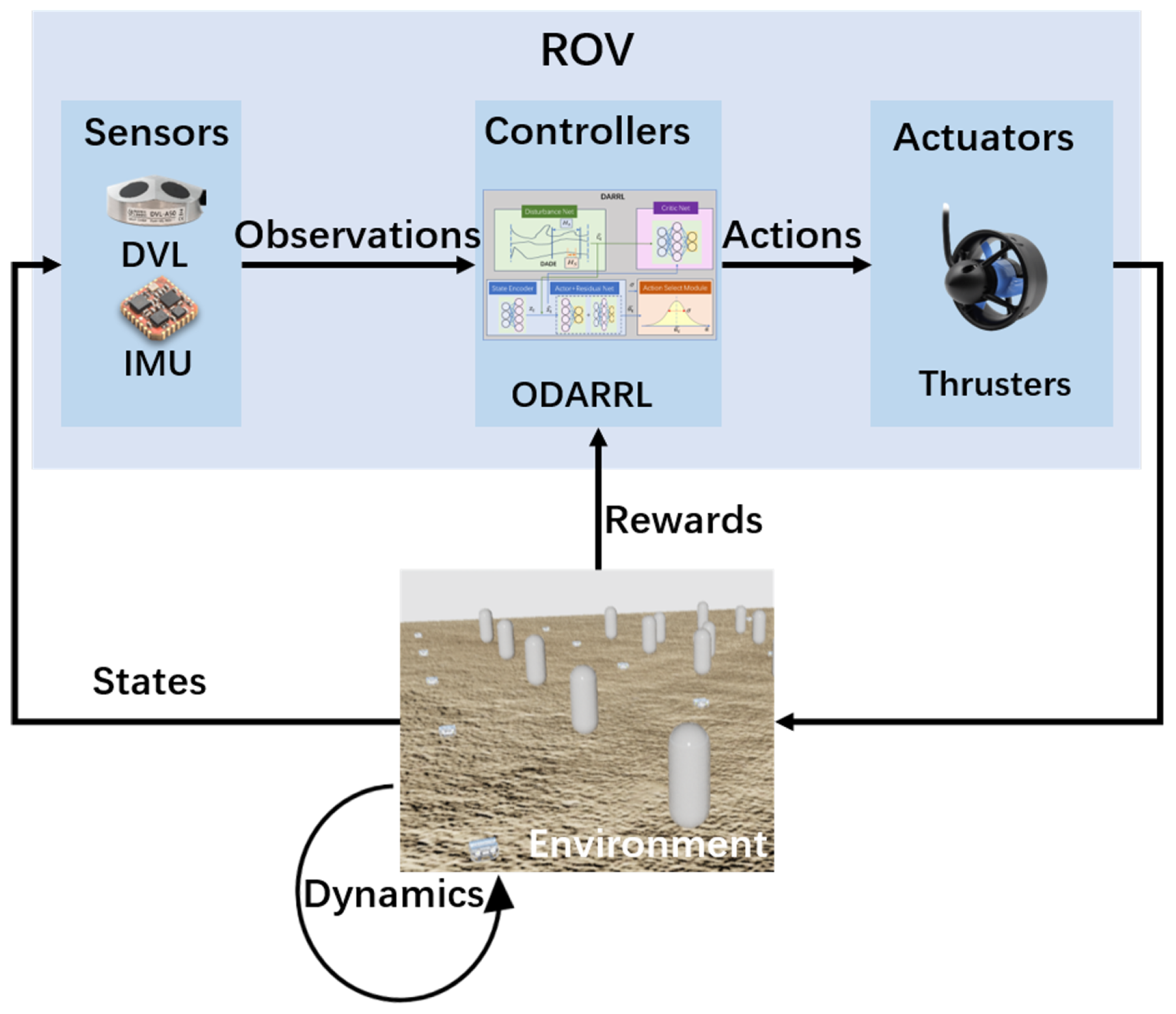
The reinforcement learning agent learns a control policy that maps observations to actions through continuous interaction with the environment. As shown in Figure 2, at each time step t, the agent first receives the current observation $o_t$, then selects an action $a_t$ according to the policy, and applies it to the environment. After the action is executed, the environment evolves to the next time step, and the agent receives the immediate reward $r_t$ together with a new observation $o_{t+1}$. By continuously interacting with the environment during training and optimizing the policy according to the obtained returns, the agent progressively learns a control policy that maximizes the expected cumulative discounted return.

3. Methodology

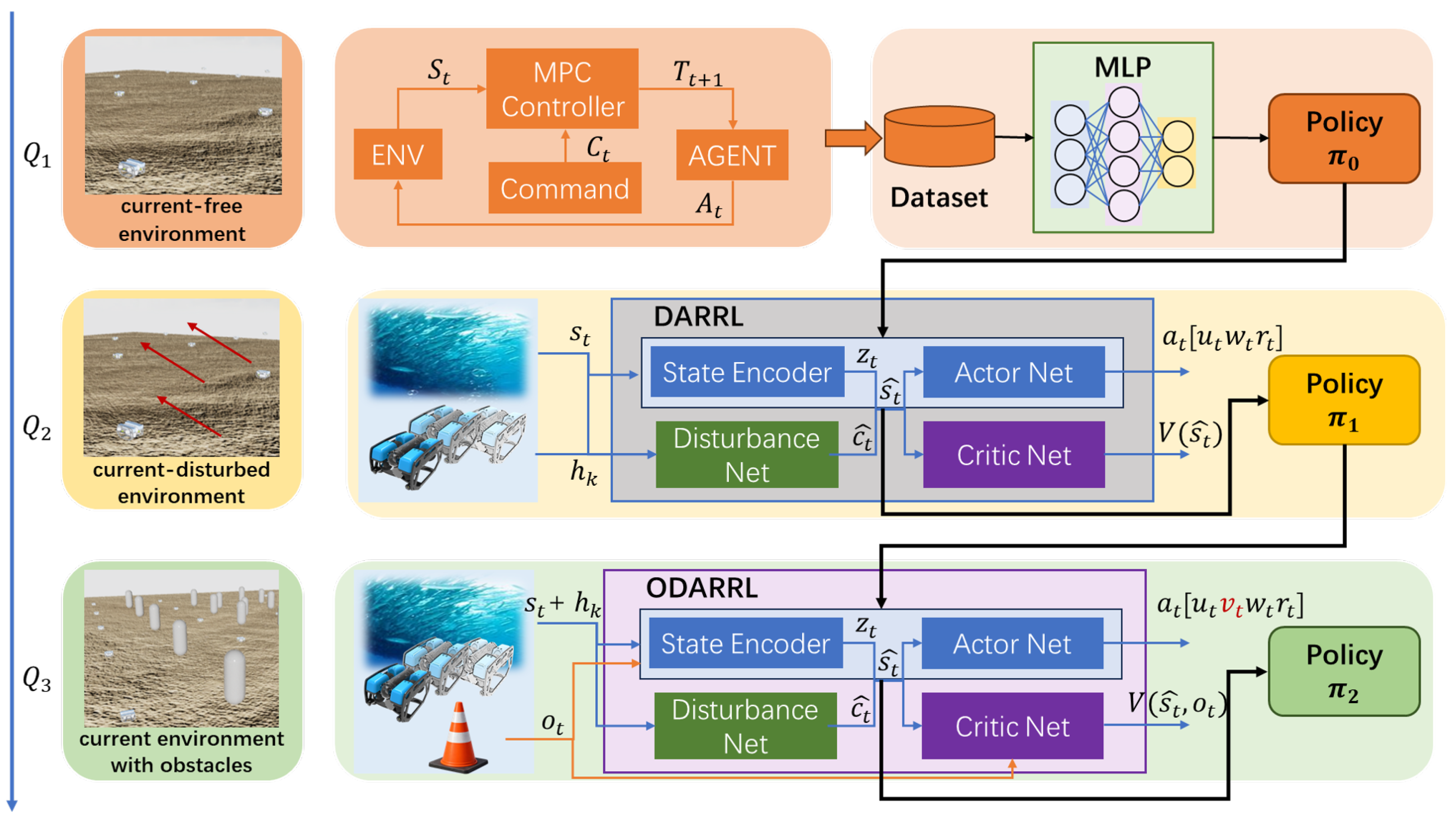
In this section, the proposed Obstacle- and Disturbance-Aware end-to-end Residual Reinforcement Learning (ODARRL) framework for underwater robot trajectory tracking with obstacle avoidance, is presented. ODARRL is designed as a three-stage curriculum learning framework for safe trajectory execution of underwater robots, and its overall pipeline is illustrated in Figure 3. Following an easy-to-hard and prior-guided-to-interaction-driven design principle, the policy learning process is progressively expanded from basic trajectory execution to disturbance-aware tracking and finally to obstacle-aware safe execution in complex underwater environments. The stage progression can be summarized as

$${\mathcal{T}}^{\left(1\right)}\prec {\mathcal{T}}^{\left(2\right)}\prec {\mathcal{T}}^{\left(3\right)},$$

(14)

and the corresponding policy evolution is given by

$${\pi }_0\to {\pi }_1\to {\pi }_2.$$

(15)

In the first stage, the robot operates in a simplified environment without currents or obstacles. Since direct training of a thruster-level end-to-end policy from scratch suffers from a large search space, slow convergence, and unstable optimization, an MPC controller is first used to generate demonstration data in the disturbance-free environment. An initial policy ${\pi }_0$ is then obtained through imitation learning. The purpose of this stage is not to derive the final controller directly, but to transfer the structured control knowledge of the classical controller in a simple environment into the learning policy, thereby providing a stable and feasible starting point for subsequent reinforcement learning.

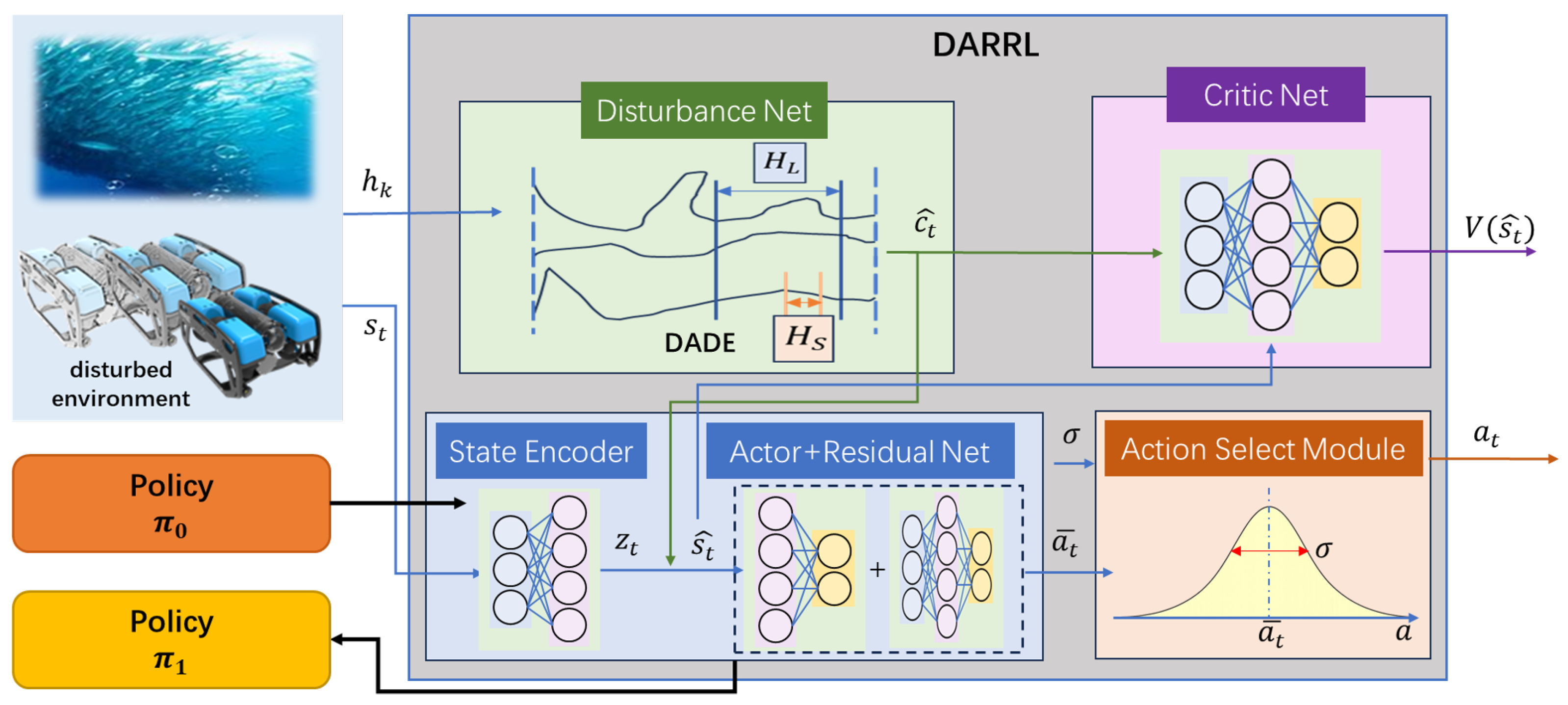
In the second stage, the environment is extended to a scenario with random current disturbances but without obstacles. The imitation-learned policy ${\pi }_0$ obtained in Stage I is transferred to Stage II and retained as a frozen base policy, whose parameters are not updated during subsequent reinforcement learning. A trainable residual branch, consisting of a state encoder, a disturbance representation module, a residual actor, and a critic, is introduced to learn disturbance-compensation actions from the current state and historical observations. The frozen base action and the learned residual correction are combined to construct the disturbance-aware policy ${\pi }_1$.

In the third stage, the environment is further extended to a complex scenario containing both current disturbances and obstacles, which yields the final ODARRL framework. Besides the robot state and disturbance-related historical information, the policy additionally receives obstacle-related observations, so that disturbance compensation and obstacle avoidance can be considered simultaneously during trajectory execution. The state encoder and the disturbance representation module learned in the previous stage are retained, while obstacle perception is incorporated into the actor–critic structure to support safe action selection in locally constrained environments. Through this progressive training procedure, the policy evolves from the imitation-based initialization policy ${\pi }_0$ to the disturbance-aware policy ${\pi }_1$, and finally to the obstacle- and disturbance-aware policy ${\pi }_2$.

Overall, the design of ODARRL reflects the coordination of three complementary components. First, MPC-guided imitation learning alleviates the difficulty of training from scratch by providing a feasible initialization policy. Second, disturbance-aware representation learning improves the ability of the policy to identify and compensate for the effects of random currents. Third, curriculum-based task expansion enables smooth transfer from basic trajectory execution to safe trajectory execution in complex underwater environments. Based on this overall framework, the following subsections introduce the policy initialization process, the design of the disturbance encoder, the structure of DARRL, and the stage-wise training mechanism in detail.

3.1. MPC-Guided Policy Initialization via Imitation Learning

In the first stage, an initial policy is obtained through imitation learning in a simplified environment without currents or obstacles. The motivation for introducing this stage is that direct training of a thruster-level end-to-end policy from scratch usually encounters a large continuous action space, unstable exploration, and low sample efficiency. To alleviate these difficulties, an MPC controller is employed as the expert controller to provide structured demonstration data for policy initialization.

Specifically, in the disturbance-free environment, the robot interacts with the environment under the control of the MPC controller. At each time step t, the controller receives the current robot state together with reference-related commands, and produces an expert control action by solving the corresponding constrained optimization problem. By rolling out this expert controller over multiple reference trajectories, the following demonstration dataset can be constructed:

$${\mathcal{D}}_{\mathrm{IL}}={\left\{(x_t,a_t^{\mathrm{MPC}})\right\}}_{t=1}^N,$$

(16)

where $x_t$ denotes the policy input at time step t, which contains the robot state and reference-related information, and $a_t^{\mathrm{MPC}}$ denotes the control action generated by the MPC controller.

After the demonstration dataset is obtained, a multilayer perceptron (MLP) is trained to approximate the expert policy through behavioral cloning. Let the initial policy be denoted by ${\pi }_0(·)$. The objective of imitation learning is then formulated as

$${\mathcal{L}}_{\mathrm{IL}}={\displaystyle \frac{1}{N}}{\displaystyle \sum _{t=1}^N}{∥{\pi }_0\left(x_t\right)-a_t^{\mathrm{MPC}}∥}_2^2,$$

(17)

which minimizes the mean squared error between the policy output and the expert action over the entire demonstration dataset. After supervised training, the resulting policy ${\pi }_0$, hereafter referred to as the MPC-imitation policy, is able to reproduce the basic control behavior of the MPC controller in the simplified environment. It should be emphasized that the MPC expert controller and ${\pi }_0$ are two different controllers: the former solves an online optimization problem and is used to generate expert demonstrations, whereas the latter is a neural policy trained through behavioral cloning and does not perform online MPC optimization.

It should be emphasized that ${\pi }_0$ is not regarded as the final controller. Instead, it serves as a feasible and stable initialization policy for the subsequent reinforcement learning stages. In this way, the policy can inherit the structured control prior contained in the expert demonstrations, thereby effectively reducing the search space of subsequent learning and improving the stability of further optimization in disturbed environments. Therefore, the first stage provides a reliable starting point for the transition from expert-guided control to interaction-driven policy refinement.

3.2. Dual-Horizon Attention Disturbance Encoder

The influence of ocean currents on the motion of the robot body is usually difficult to identify from the observation at a single time step, and instead depends more strongly on temporal patterns reflected by a history of state evolution. To address this issue, a Dual-Horizon Attention Disturbance Encoder (DADE) is designed to extract disturbance-related representation features from historical observations and to provide explicit disturbance-aware information for subsequent policy learning.

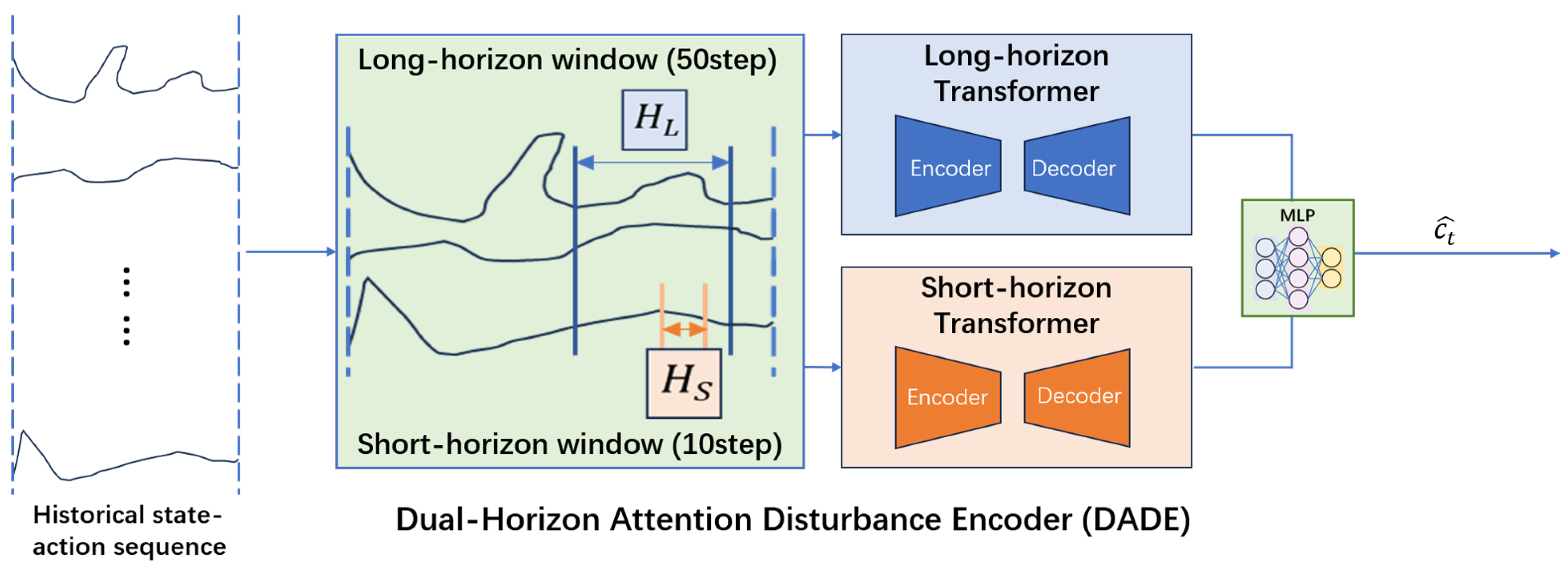
As shown in Figure 4, DADE divides the historical observation sequence into two temporal windows with different scales, namely a long-horizon window and a short-horizon window. The long-horizon window is used to capture slowly varying trends induced by ocean currents over an extended period, whereas the short-horizon window focuses on transient variations and rapid fluctuations within a local temporal range. Through this dual-horizon design, the encoder can simultaneously account for the long-term accumulated effect of disturbances and the short-term dynamic response, thereby improving the representation capability for complex underwater disturbances. Let the short-horizon and long-horizon observation sequences at time step t be denoted by

$$h_t^S=\{o_{t-T_S+1},\dots ,o_t\},h_t^L=\{o_{t-T_L+1},\dots ,o_t\},$$

(18)

where $T_S$ and $T_L$ denote the lengths of the short-horizon and long-horizon windows, respectively.

For each temporal window, a Transformer-based [34] temporal encoder is adopted to model the input sequence. Compared with temporal modeling methods that rely only on local convolution or fixed recurrent structures, the Transformer can capture cross-time-step dependencies more effectively and is therefore well suited for extracting disturbance-related temporal features from historical observations. Specifically, the long-horizon branch and the short-horizon branch perform embedding projection and attention-based encoding on the corresponding input sequences, yielding two temporal feature representations:

$$z_t^S=\mathrm{Pool}\left({\mathrm{Transformer}}_S\left({\mathrm{Embed}}_S\left(h_t^S\right)\right)\right),$$

(19)

$$z_t^L=\mathrm{Pool}\left({\mathrm{Transformer}}_L\left({\mathrm{Embed}}_L\left(h_t^L\right)\right)\right),$$

(20)

where $z_t^S$ and $z_t^L$ denote the pooled short-horizon and long-horizon temporal features, respectively. The outputs of the two branches are then fused by an MLP to generate the final disturbance-aware feature:

$${\widehat{c}}_t=f_{\mathrm{fuse}}\left([z_t^S;z_t^L]\right),$$

(21)

where $[·;·]$ denotes feature concatenation.

It should be emphasized that ${\widehat{c}}_t$ does not correspond to any explicitly observable current variable. Instead, it is an equivalent disturbance representation for control decision-making, which characterizes the overall influence of ocean currents on the robot motion under the current historical context. In the subsequent DARRL framework, ${\widehat{c}}_t$ is combined with the state encoding feature as the input of the policy network and the value network. In this way, the policy can explicitly utilize historical disturbance information during decision-making, rather than relying only on the instantaneous state for action selection.

In the implementation, the length of the short-horizon window is set to 10 time steps, and the length of the long-horizon window is set to 50 time steps. Each branch contains one Transformer encoder layer, with an input embedding dimension of 64, four attention heads, a feed-forward network dimension of 128, and a dropout rate of 0.1. To obtain a fixed-dimensional temporal representation, mean pooling is adopted in both branches. The fusion MLP is configured as 128-64-64, and the final output is a disturbance-aware feature with dimension 64. The corresponding hyperparameter settings are summarized in

Table 1. Hyperparameter configuration of the proposed DADE module.

Parameter	Configuration
Short-horizon window	10 steps
Long-horizon window	50 steps
Input embedding dimension	64
Attention heads	4
Feed-forward dimension	128
Dropout	0.1
Pooling	Mean pooling
Fusion MLP	128-64-64
Disturbance feature dimension	64

.

3.3. Disturbance-Aware Residual Reinforcement Learning

Based on the initial policy ${\pi }_0$ obtained through imitation learning, the second stage introduces Disturbance-Aware Residual Reinforcement Learning (DARRL) to improve the robustness of trajectory execution under random current disturbances. As shown in Figure 5, DARRL consists of four main components, namely a state encoder, a disturbance representation module, an actor network, and a critic network. The core objective of DARRL is not to update or replace the imitation-learned policy ${\pi }_0$, but to retain it as a frozen base policy and learn an additional disturbance-aware residual correction. Therefore, the parameters of ${\pi }_0$ remain fixed throughout Stage-II training, whereas the newly introduced residual-learning components are optimized to construct the disturbance-aware policy ${\pi }_1$.

At each time step t, the robot first receives the current state $s_t$ together with the corresponding historical observation sequence $h_t$. The current state is mapped by the state encoder into a compact state feature,

$$z_t=f_{\mathrm{enc}}\left(s_t\right),$$

(22)

while the DADE module extracts a disturbance-aware feature from the historical observations, denoted by

$${\widehat{c}}_t=f_d\left(h_t\right).$$

(23)

In addition, a reference-related guidance command $c_t$ is generated at each time step according to the current robot state and the reference trajectory information, namely,

$$c_t=g(s_t,P_{\mathrm{ref}}).$$

(24)

These features are then concatenated to form the input of both the actor network and the critic network:

$${\widehat{s}}_t=[z_t,c_t,{\widehat{c}}_t].$$

(25)

Under this construction, the policy no longer makes decisions only from the encoded instantaneous state. Instead, it jointly exploits the inferred disturbance effect and the reference-related command, thereby enabling adaptive control under random current disturbances.

Rather than directly replacing the initialized policy, DARRL adopts a residual policy learning formulation. Let ${\pi }_0\left(x_t\right)$ denote the frozen base policy inherited from Stage I, and let ${\pi }_{\theta }(·\mid {\widehat{s}}_t)$ denote the trainable residual actor introduced in Stage II. The final control action is defined as

$$a_t=a_t^{\mathrm{base}}+\Delta a_t,a_t^{\mathrm{base}}={\pi }_0\left(x_t\right).$$

(26)

where the residual correction term is sampled from the residual actor,

$$\Delta a_t\sim {\pi }_{\theta }(·\mid {\widehat{s}}_t).$$

(27)

Equivalently, the deployed disturbance-aware policy can be written as

$${\pi }_1(x_t,h_t)={\pi }_0\left(x_t\right)+{\pi }_{\theta }\left({\widehat{s}}_t\right),{\widehat{s}}_t=[z_t,c_t,{\widehat{c}}_t].$$

(28)

Under this formulation, the parameters of ${\pi }_0$ remain fixed, thereby preserving the basic trajectory-execution behavior learned from the MPC demonstrations. The trainable residual branch uses the encoded state, reference command, and DADE feature to compensate for deviations induced by current disturbances.

To optimize the residual actor, DARRL adopts a PPO-based actor–critic framework. The actor network outputs the residual action distribution conditioned on ${\widehat{s}}_t$, whereas the critic network estimates the value function $V_{\psi }\left({\widehat{s}}_t\right)$ for policy evaluation. Following the PPO formulation, the residual actor is updated by maximizing the clipped surrogate objective

$$L^{\mathrm{clip}}\left(\theta \right)={\mathbb{E}}_t\left[min\left(r_t\left(\theta \right){\widehat{A}}_t,\mathrm{clip}\left(r_t\left(\theta \right),1-ϵ,1+ϵ\right){\widehat{A}}_t\right)\right],$$

(29)

where

$$r_t\left(\theta \right)={\displaystyle \frac{{\pi }_{\theta }(\Delta a_t\mid {\widehat{s}}_t)}{{\pi }_{{\theta }_{\mathrm{old}}}(\Delta a_t\mid {\widehat{s}}_t)}}.$$

(30)

Here, ${\widehat{A}}_t$ denotes the estimated advantage function, and $ϵ$ is the clipping parameter used to limit the magnitude of policy updates. The training procedure of DARRL is summarized in Algorithm 1.

After training in this stage, the resulting policy ${\pi }_1$ serves as the disturbance-aware control policy obtained in the second stage. Compared with the initialization policy ${\pi }_0$ learned by imitation learning, ${\pi }_1$ can explicitly utilize temporal disturbance representations together with residual correction, thereby improving the ability of adaptive compensation in random current environments. The overall training procedure of the third stage is largely identical to that of the second stage, except that obstacle observations are additionally introduced. Therefore, the details are omitted here.

Algorithm 1 Disturbance-Aware Residual Reinforcement Learning (DARRL)

Input: Disturbed environment $\mathcal{E}$, command generator $g(·)$, state encoder $f_{\mathrm{enc}}(·)$, disturbance estimator $f_d(·)$, base imitation policy ${\pi }_0$, residual actor ${\pi }_{\theta }$, critic $V_{\psi }$, PPO hyperparameters $(H,K,B,\gamma ,\lambda )$ Output: Trained residual policy ${\pi }_{\theta }$ and deployed policy ${\pi }_1$ Freeze base imitation policy ${\pi }_0$ Initialize residual actor parameters $\theta$ Initialize critic parameters $\psi$ Initialize disturbance network parameters $\omega$ for each iteration do     Reset environment and obtain initial state $s_0$     Initialize rollout buffer $\mathcal{D}\leftarrow \varnothing$     for $t=0$ to $H-1$ do         Generate nominal command $c_t=g\left(s_t\right)$         Encode state feature $z_t=f_{\mathrm{enc}}\left(s_t\right)$         Estimate disturbance feature ${\widehat{c}}_t=f_d\left(h_t\right)$         Construct observation ${\widehat{s}}_t=[z_t,c_t,{\widehat{c}}_t]$         Compute the frozen base action $a_t^{\mathrm{base}}={\pi }_0\left(x_t\right)$         Sample residual action $\Delta a_t\sim {\pi }_{\theta }(·\mid {\widehat{s}}_t)$         Compose final action $a_t=a_t^{\mathrm{base}}+\Delta a_t$         Execute $a_t$ in $\mathcal{E}$ and observe $r_t,s_{t+1}$         Store $({\widehat{s}}_t,\Delta a_t,a_t,r_t,s_{t+1})$ in $\mathcal{D}$     end for     Compute returns ${\widehat{R}}_t$ and advantages ${\widehat{A}}_t$ using GAE$(\gamma ,\lambda )$     for $k=1$ to K do         Sample mini-batch $\mathcal{B}\subset \mathcal{D}$         Update residual actor by PPO objective:              ${max}_{\theta }\mathbb{E}\left[min\left(r_t\left(\theta \right){\widehat{A}}_t,\mathrm{clip}(r_t\left(\theta \right),1-ϵ,1+ϵ){\widehat{A}}_t\right)\right]$         Update critic by minimizing:              ${\mathcal{L}}_V=\mathbb{E}\left[{(V_{\psi }\left({\widehat{s}}_t\right)-{\widehat{R}}_t)}^2\right]$         Update disturbance network jointly     end for end for Define deployed policy:       ${\pi }_1(x_t,h_t)={\pi }_0\left(x_t\right)+{\pi }_{\theta }\left({\widehat{s}}_t\right)$ return ${\pi }_1$

3.4. Training Strategy and Network Optimization

To maintain consistency of the network structure throughout the overall training process, each newly introduced disturbance-related input is represented by a corresponding zero-valued placeholder in earlier stages rather than being removed from the network input. In this work, the newly introduced factors refer to current disturbances in the second stage and obstacle observations in the third stage. This design ensures architectural consistency across stages and avoids the influence of network structure changes on training performance. Specifically, in the initialization stage, the influence of the environmental current on the robot is represented by a zero vector,

$${\widehat{c}}_t=\mathbf{0},$$

(31)

which indicates that no current disturbance is present. For obstacle perception, the observation includes not only relative position information but also a mask term. In the first two stages, the mask is always set to one, which indicates that no obstacle exists within the observable range. In this way, the input dimensionality remains unchanged across different training stages.

In the second and third stages, the policy is further optimized using a PPO-based actor–critic scheme [35]. For each rollout, the agent interacts with the environment for H time steps, and the collected transition samples are stored in the rollout buffer. Based on the collected trajectories, the advantage function is estimated using generalized advantage estimation (GAE):

$${\widehat{A}}_t={\displaystyle \sum _{l=0}^{T-t-1}}{\left(\gamma \lambda \right)}^l{\delta }_{t+l},$$

(32)

where

$${\delta }_t=r_t+\gamma V_{\psi }\left({\widehat{s}}_{t+1}\right)-V_{\psi }\left({\widehat{s}}_t\right).$$

(33)

Here, $\gamma$ denotes the discount factor, and $\lambda$ denotes the GAE coefficient. The critic network is updated by minimizing the value loss

$$L_V={\mathbb{E}}_t\left[{\left(V_{\psi }\left({\widehat{s}}_t\right)-{\widehat{R}}_t\right)}^2\right],$$

(34)

where ${\widehat{R}}_t$ denotes the estimated return. To encourage sufficient exploration during training, an entropy regularization term is further introduced. The overall optimization objective is therefore written as

$$L=-L^{\mathrm{clip}}+c_1{L}_V-c_2{L}_{\mathrm{ent}},$$

(35)

where $L^{\mathrm{clip}}$ denotes the clipped surrogate objective of PPO, $L_{\mathrm{ent}}$ denotes the entropy regularization term, and $c_1$ and $c_2$ are balancing coefficients.

During optimization, the rollout data collected in each iteration are shuffled and divided into several mini-batches, after which the actor network and the critic network are updated for multiple epochs. In the second stage, the residual branch is optimized on top of the policy initialized by imitation learning, thereby producing the disturbance-aware policy ${\pi }_1$. In the third stage, ${\pi }_1$ is further used as the initialization policy in the obstacle-constrained environment, and continued training yields the final policy ${\pi }_2$. Through this stage-wise optimization process, the policy progressively acquires basic trajectory execution capability, disturbance compensation capability, and safe control capability under obstacle constraints.

To make the stage-wise reward design explicit, the reward functions used in the second and third training stages are summarized as follows. In the second stage, the reward is defined as

$$r_t^{\left(2\right)}=w_{\mathrm{prog}}\Delta {\mathcal{l}}_t-w_{xy}{e}_t^H-w_{\mathrm{yaw}}{e}_t^{\psi }-w_z{e}_t^V,$$

(36)

where $\Delta {\mathcal{l}}_t=\mathcal{S}\left(q_t\right)-\mathcal{S}\left(q_{t-1}\right)$ denotes the path-progress increment along the reference trajectory, $e_t^H$ and $e_t^V$ denote the horizontal and vertical tracking errors, respectively, and

$$e_t^{\psi }=\left|\mathrm{wrap}({\psi }_t-{\psi }_t^{*})\right|$$

(37)

denotes the yaw-tracking error with respect to the reference path direction. This reward encourages effective advancement along the reference path while penalizing planar deviation, depth error, and yaw misalignment under current disturbances.

In the third stage, the task objective is further extended from robust trajectory tracking under random currents to safe trajectory execution under both current disturbances and obstacle constraints. In environments with obstacles, strict trajectory tracking is not always the primary objective. When an obstacle is located near the reference trajectory, a consistently strong tracking penalty may attract the policy toward the nominal path and cause the vehicle to pass excessively close to the obstacle. Therefore, a segmented obstacle-aware reward mechanism is introduced to adaptively adjust the relative importance of trajectory tracking and obstacle clearance according to the local task condition.

Let ${\mu }_t\in \{\mathrm{TRACKING},\mathrm{AVOIDING},\mathrm{RECOVERING}\}$ denote the reward mode at time step t. The mode transition follows

$$\mathrm{TRACKING}\to \mathrm{AVOIDING}\to \mathrm{RECOVERING}\to \mathrm{TRACKING}.$$

(38)

In the $\mathrm{TRACKING}$ mode, no relevant forward obstacle is detected within the local activation range, and the policy focuses on tracking the reference trajectory. When a relevant obstacle enters the activation range, lies ahead of the current path progress, and intersects the safety corridor of the reference trajectory, the system switches to the $\mathrm{AVOIDING}$ mode. In this mode, the tracking penalties are temporarily reduced, while path progress, clearance growth, and safety-shortfall penalties are emphasized. After the obstacle is classified as passed, the system enters the $\mathrm{RECOVERING}$ mode, where the tracking penalties are gradually restored to avoid abrupt control changes after obstacle avoidance.

Let $s_t$ denote the projected progress of the vehicle along the reference trajectory, $s_{\mathrm{obs}}$ denote the projected progress of the obstacle center along the reference trajectory, $d_{\mathrm{obs},t}$ denote the horizontal center distance between the vehicle and the active obstacle, and $c_{\mathrm{obs},t}$ denote the horizontal surface clearance from the obstacle. An obstacle is activated when

$$\begin{array}{cc}\hfill d_{\mathrm{obs},t}& <d_{\mathrm{act}},\hfill \\ \hfill s_{\mathrm{obs}}& >s_t,\hfill \\ \hfill d(p_{\mathrm{obs}},\mathsf{\Gamma })& <r_{\mathrm{obs}}+d_{\mathrm{safe}},\hfill \end{array}$$

(39)

and the obstacle has not been passed previously. Here, $\mathsf{\Gamma }$ denotes the reference trajectory, $d_{\mathrm{act}}$ is the obstacle activation distance, $r_{\mathrm{obs}}$ is the obstacle radius, and $d_{\mathrm{safe}}$ is the target safety clearance. Once activated, the obstacle is locked as the active obstacle until it is classified as passed, which prevents mode chattering near the activation boundary.

The active obstacle is considered to be passed when

$$\begin{array}{cc}\hfill s_t& >s_{\mathrm{obs}}+{\Delta }_{\mathrm{pass}},\hfill \\ \hfill c_{\mathrm{obs},t}& >d_{\mathrm{pass}},\hfill \\ \hfill d_{\mathrm{obs},t}-d_{\mathrm{obs},t-1}& >{ϵ}_d,\hfill \end{array}$$

(40)

where

$${\Delta }_{\mathrm{pass}}=r_{\mathrm{obs}}+d_{\mathrm{safe}}+d_{\mathrm{margin}}.$$

(41)

These conditions require the vehicle not only to move laterally away from the obstacle, but also to advance beyond the obstacle along the reference-path direction and continue moving away from it. Compared with a simple distance-based criterion, this progress-based pass condition more reliably determines whether the vehicle has truly passed the obstacle or has merely moved to its side.

After the obstacle is classified as passed, a half-cosine schedule is used in the $\mathrm{RECOVERING}$ mode to smoothly restore the tracking-penalty weights:

$$\beta \left(k\right)={\displaystyle \frac{1-\cos (\pi k/N_{\mathrm{rec}})}{2}},0\le k\le N_{\mathrm{rec}},$$

(42)

$${\alpha }_{xy}\left(k\right)={\alpha }_{xy}^A+(1-{\alpha }_{xy}^A)\beta \left(k\right),$$

(43)

$${\alpha }_{\mathrm{yaw}}\left(k\right)={\alpha }_{\mathrm{yaw}}^A+(1-{\alpha }_{\mathrm{yaw}}^A)\beta \left(k\right).$$

(44)

Here, k is the number of elapsed steps in the $\mathrm{RECOVERING}$ mode, $N_{\mathrm{rec}}$ is the recovery duration, and ${\alpha }_{xy}^A$ and ${\alpha }_{\mathrm{yaw}}^A$ are the tracking-penalty scaling factors used in the $\mathrm{AVOIDING}$ mode. When both scaling factors reach one, or when the horizontal tracking error becomes smaller than the threshold $e_{\mathrm{rec}}$, the system switches back to the $\mathrm{TRACKING}$ mode.

Accordingly, the third-stage reward is formulated as a mode-dependent function:

$$r_t^{\left(3\right)}=\left\{\begin{array}{cc}{r}_t^{\mathrm{trk}},\hfill & {\mu }_t=\mathrm{TRACKING},\hfill \\ r_t^{\mathrm{avo}},\hfill & {\mu }_t=\mathrm{AVOIDING},\hfill \\ r_t^{\mathrm{rec}},\hfill & {\mu }_t=\mathrm{RECOVERING}.\hfill \end{array}\right.$$

(45)

In the $\mathrm{TRACKING}$ mode, the reward retains the same tracking-oriented structure as the second-stage reward:

$$r_t^{\mathrm{trk}}=w_{\mathrm{prog}}\Delta {\mathcal{l}}_t-w_{xy}{e}_t^H-w_{\mathrm{yaw}}{e}_t^{\psi }-w_z{e}_t^V.$$

(46)

In the $\mathrm{AVOIDING}$ mode, the reward is defined as

$$\begin{array}{cc}\hfill r_t^{\mathrm{avo}}=& w_{\mathrm{prog}}\Delta {\mathcal{l}}_t^{+}+w_{\mathrm{prog}}^A\Delta {\mathcal{l}}_t^{+}+w_{\Delta d}\Delta d_t^{+}-w_{xy}{\alpha }_{xy}^A{e}_t^H\hfill \\ \hfill & -w_{\mathrm{yaw}}{\alpha }_{\mathrm{yaw}}^A{e}_t^{\psi }-w_z{e}_t^V-w_{\mathrm{obs}}{q}_{\mathrm{safe}}-w_{\mathrm{entry}}{I}_{\mathrm{entry}},\hfill \end{array}$$

(47)

where $\Delta {\mathcal{l}}_t^{+}=max(\Delta {\mathcal{l}}_t,0)$ denotes the positive path-progress increment, $\Delta d_t^{+}=max(d_{\mathrm{obs},t}-d_{\mathrm{obs},t-1},0)$ denotes the positive increase in the distance from the active obstacle, and $I_{\mathrm{entry}}$ is an event indicator that is activated only when the vehicle first enters the safety zone of the active obstacle. The safety-shortfall penalty is defined as

$$q_{\mathrm{safe}}=\mathrm{clip}{\left({\displaystyle \frac{d_{\mathrm{safe}}-c_{\mathrm{obs},t}}{d_{\mathrm{safe}}}},0,3\right)}^2.$$

(48)

It should be noted that $d_{\mathrm{safe}}$ denotes the target clearance encouraged by the reward function, rather than a hard safety guarantee.

In the $\mathrm{RECOVERING}$ mode, the reward is defined as

$$r_t^{\mathrm{rec}}=w_{\mathrm{prog}}\Delta {\mathcal{l}}_t-w_{xy}{\alpha }_{xy}\left(k\right)e_t^H-w_{\mathrm{yaw}}{\alpha }_{\mathrm{yaw}}\left(k\right)e_t^{\psi }-w_z{e}_t^V.$$

(49)

Sparse event rewards or penalties, including obstacle-pass bonuses, collision penalties, avoidance-stall penalties, and goal-reaching bonuses, are handled by the event-detection and termination logic of the environment. These terms are omitted from the compact reward expressions above for clarity. The main training hyperparameters of the second stage are summarized in

Table 2. Parameters used in Stage-II training.

Symbol	Description	Value
$v_{\mathrm{ref}}$	Reference speed	0.85 m/s
$L_{\mathrm{path}}$	Path length	35.0 m
$N_w$	Reference window length	20
$d_{\mathrm{la}}$	Path look-ahead distance	1.5 m
$[V_{min},V_{max}]$	Ocean current speed range	$[0.2,0.4]$ m/s
${\theta }_c$	Ocean current direction	Random
${\alpha }_p$	Planar residual coefficient	0.1
${\alpha }_v$	Vertical residual coefficient	0.05
$N_{\mathrm{env}}$	Number of parallel environments	64
T	Rollout steps	1024
K	PPO epochs	4
$N_{\mathrm{mb}}$	Number of minibatches	64
${\eta }_a$	Actor learning rate	$1.5\times {10}^{-4}$
${\eta }_c$	Critic learning rate	$1.5\times {10}^{-4}$
$\gamma$	Discount factor	0.99
$\lambda$	GAE parameter	0.95
$ϵ$	PPO clip parameter	0.15
$c_e$	Entropy coefficient	$5\times {10}^{-4}$
$w_{\mathrm{prog}}$	Progress reward weight	15.0
$w_{xy}$	XY error penalty weight	2.0
$w_{\mathrm{yaw}}$	Yaw error penalty weight	0.8
$w_z$	Depth error penalty weight	0.1

, while the additional parameters introduced in the third stage are listed in

Table 3. Key parameters used in Stage-III obstacle-aware training.

Symbol	Description	Value
$N_{\mathrm{obs}}$	Number of obstacles	2
$P_{\mathrm{obs}}$	Relative obstacle positions along path	$[0.35,0.68]$
$d_{\det }$	Obstacle detection range	5.0 m
$R_{\mathrm{obs}}$	Obstacle radius	0.45 m
$d_{\mathrm{safe}}$	Target obstacle-surface clearance	0.8 m
$d_{\mathrm{pass}}$	Pass-decision clearance	0.6 m
$d_{\mathrm{margin}}$	Additional pass-progress margin	0.5 m
$\Delta s_{\mathrm{pass}}$	Pass-progress offset	1.75 m
$N_{\mathrm{rec}}$	Recovery duration	100 steps
$e_{\mathrm{rec}}$	Early recovery-error threshold	0.35 m
${\alpha }_{xy}^A$	XY-tracking scale in AVOIDING	0.15
${\alpha }_{\mathrm{yaw}}^A$	Yaw-tracking scale in AVOIDING	0.10
$w_{\mathrm{prog}}^A$	Additional avoidance-progress weight	80.0
$w_{\Delta d}$	Clearance-growth reward weight	6.0
$w_{\mathrm{obs}}$	Safety-shortfall penalty weight	6.0
$w_{\mathrm{entry}}$	Safety-zone entry penalty weight	4.0
$w_{\mathrm{col}}$	Collision penalty weight	50.0

.

4. Simulation, Results and Analysis

This section presents a systematic simulation-based validation and performance analysis of the proposed ODARRL framework. All experiments were conducted on the Marine Gym platform, with BlueROV2 Heavy used as the controlled robotic platform. First, the simulation environment, task settings, and evaluation metrics are introduced. Then, under random current disturbance scenarios, DARRL is compared with baseline methods, including MPC-imitation policy, PPO, SAC, A2C and VNRS-SAC, in order to verify its advantages in trajectory execution accuracy and robustness. On this basis, the obstacle-avoidance capability and training efficiency of the proposed three-stage curriculum learning framework are further evaluated in environments with obstacles.

4.1. Simulation Platform and Experimental Setup

All experiments in this study were conducted on the MarineGym v1.0 platform, with BlueROV2 Heavy used as the controlled underwater robotic platform. Marine Gym provides a high-performance underwater simulation environment for reinforcement learning and supports robot dynamics, current disturbances, obstacle interaction, and parallel multi-episode sampling. A sensor-to-thruster (ST) end-to-end control setting was adopted, in which the policy directly output continuous thruster-level control commands.In addition, the vehicle mass was randomized at the beginning of each training episode to expose the policy to payload variations and model uncertainty. This setting was used to evaluate the effectiveness of the proposed method in closed-loop control at the execution layer.

To match the three-stage curriculum learning framework of ODARRL, the experimental tasks are organized into three progressively more challenging scenarios. The first stage corresponds to a basic trajectory execution task without currents or obstacles, and is used to collect expert demonstrations from the MPC controller and to train the imitation-initialized policy ${\pi }_0$. The second stage introduces random current disturbances in order to evaluate the robustness of DARRL under disturbed conditions and to obtain the disturbance-aware policy ${\pi }_1$. The third stage further introduces obstacles into the current-disturbed environment, and is used to train and evaluate the final ODARRL policy ${\pi }_2$, thereby verifying the effectiveness of stage-wise policy transfer in complex tasks.

In the simulation environment, the reference trajectory is generated as a smooth spatial curve from randomly sampled key points. To avoid unrealistically sharp turns that rarely occur in practical underwater operations, a three-dimensional extension of the quadratic polynomial interpolation (QPMI) method is adopted [36]. Current disturbances are randomly sampled at the beginning of each episode, with both magnitude and direction varying within predefined ranges, while remaining fixed during the same episode to simulate unknown ocean currents acting on the robot. In the third-stage task, several obstacles are further placed in the environment to construct obstacle-constrained scenarios. An episode is regarded as a collision failure once physical contact occurs between the robot and an obstacle. All methods are trained and evaluated under the same environment distribution and task settings in order to ensure a fair comparison. Detailed configurations of the reference trajectory, current field, and obstacle settings are summarized in Table 2 and Table 3.

To evaluate the performance of the proposed method, DARRL in the second stage is compared with PPO, SAC, A2C, VNRS-SAC and the imitation-initialized policy ${\pi }_0$. In the third stage, ODARRL initialized from ${\pi }_1$, ODARRL initialized from ${\pi }_0$, and ODARRL trained from scratch are compared in obstacle-involved environments. Through this stage-wise comparison protocol, the contributions of policy initialization, disturbance-aware residual learning, and stage-wise transfer to obstacle-constrained environments can be evaluated separately.

The evaluation metrics mainly include horizontal tracking error, vertical tracking error, total tracking error, and total RMSE, which are used to measure tracking accuracy in current-disturbed environments without obstacles. Let the robot position at time step t be denoted by

$$p_t=(x_t,y_t,z_t),$$

(50)

and let the nearest point on the reference trajectory $\mathsf{\Gamma }$ be

$$q_t=(x_t^{*},y_t^{*},z_t^{*})=\arg \underset{q\in \mathsf{\Gamma }}{min}{\parallel p_t-q\parallel }_2.$$

(51)

The horizontal, vertical, and total tracking errors are then defined as

$$e_t^H=\sqrt{{(x_t-x_t^{*})}^2+{(y_t-y_t^{*})}^2},$$

(52)

$$e_t^V=|z_t-z_t^{*}|,$$

(53)

$$e_t^T={\parallel p_t-q_t\parallel }_2.$$

(54)

Over N sampled time steps, the total RMSE is computed as

$${\mathrm{RMSE}}_T=\sqrt{{\displaystyle \frac{1}{N}}\sum _{t=1}^N{\left(e_t^T\right)}^2}.$$

(55)

In obstacle-involved environments, path progress is further introduced to quantify the effective advancement of the robot along the reference path. In addition to representative single-trajectory visualizations, all quantitative results are reported over multiple independent evaluations in order to reduce randomness and to provide a more objective assessment of the overall performance of each method.

4.2. Stage-I MPC-Guided Policy Initialization

This subsection first evaluates the effectiveness of the MPC-guided policy initialization in the first stage. The purpose of this stage is not to outperform the expert controller in the disturbance-free environment, but rather to examine whether the imitation-initialized policy ${\pi }_0$ can reproduce the control behavior of MPC in the basic trajectory execution task with sufficient fidelity, thereby providing a feasible initialization for the subsequent reinforcement learning stages.

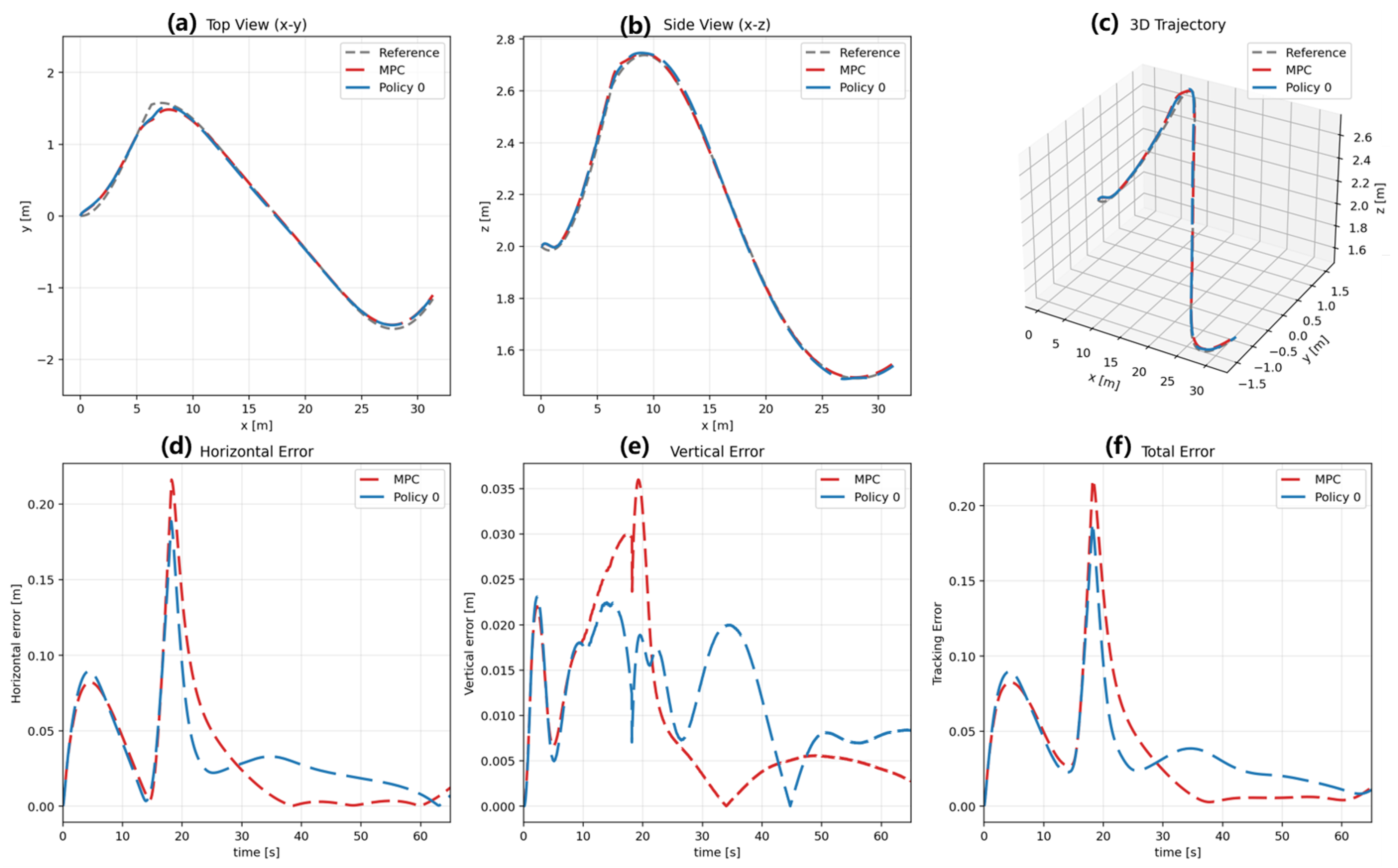
The demonstration dataset contains 50 rollout trajectories with 250,000 samples in total, among which 200,000 samples are used for training and 50,000 samples are used for validation. The best validation loss reaches 0.00394, indicating that the learned policy can closely reproduce the expert actions. As shown in Figure 6, the trajectory tracking performance of the MPC controller and the imitation-initialized policy ${\pi }_0$ is compared in the environment without currents or obstacles. Figure 6a–c present the top view, side view, and three-dimensional trajectory, respectively. It can be observed that the overall motion of ${\pi }_0$ remains highly consistent with that of the MPC controller, and the robot can stably advance along the reference path. Figure 6d–f further show the horizontal error, vertical error, and total error, respectively. The results indicate that ${\pi }_0$ is able to follow the reference trajectory well throughout the execution process. Except for the turning region, the tracking error remains below 0.05 m during most of the trajectory, and no obvious divergence or instability is observed. This result suggests that, by generating demonstration data from MPC in a simplified environment and performing behavioral cloning, the learned initialization policy has already captured the main control of the basic trajectory execution task.

Therefore, the first-stage experiment verifies the effectiveness of MPC-guided imitation learning for policy initialization. The resulting policy ${\pi }_0$ can serve as the starting point of the disturbance-aware residual reinforcement learning stage and provides a stable initialization basis for subsequent policy refinement under random current disturbances.

4.3. Stage-II Trajectory Execution Under Current Disturbances

4.3.1. Comparison with Baseline Methods

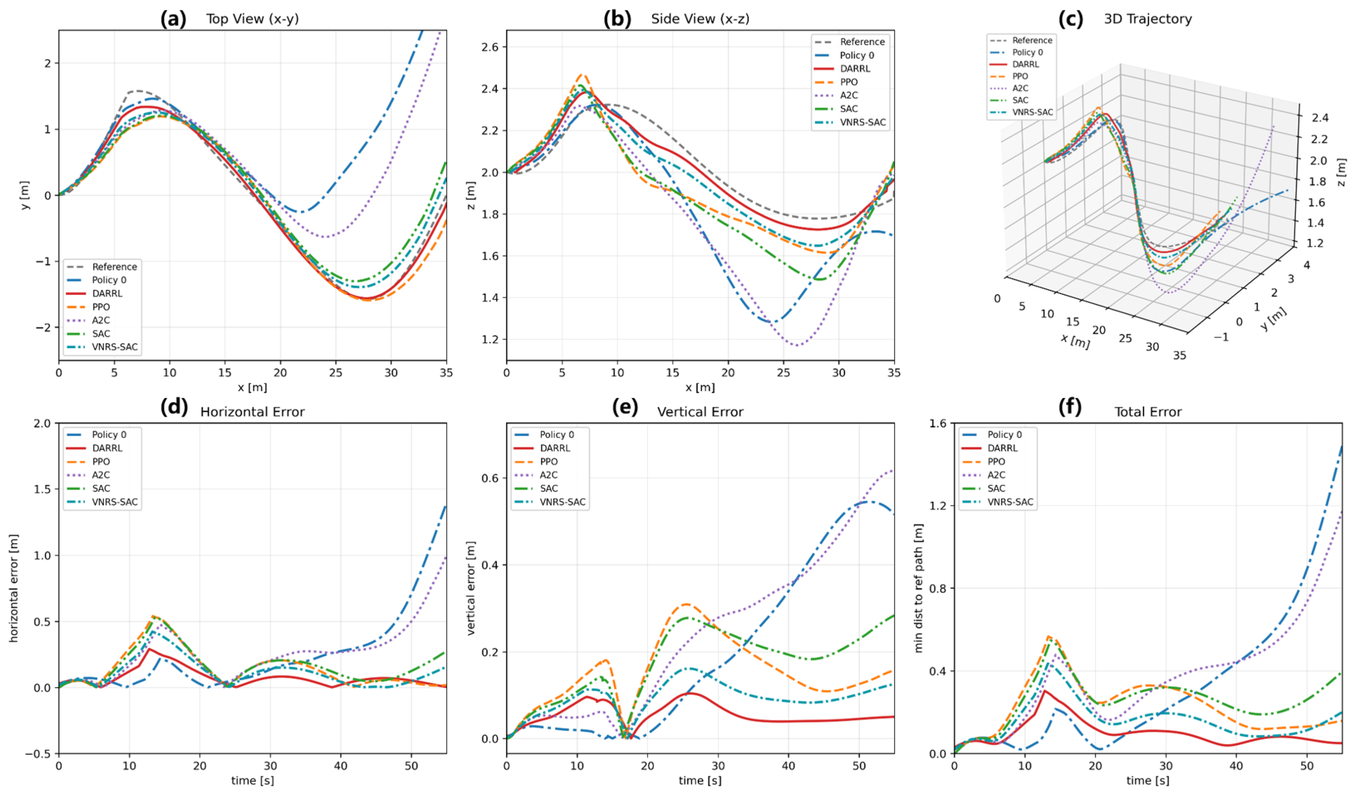
This subsection focuses on evaluating the trajectory execution performance of the proposed DARRL in the second stage under random current disturbances. Before presenting the detailed results, it should be clarified that all quantitative results in

Table 4. Test results for all controllers under current disturbances. All error metrics are reported in meters.

Controller	Horizontal Mean Error	Vertical Mean Error	Mean 3D Error	3D RMSE
DARRL	0.146	0.068	0.175	0.312
MPC-IL policy	0.514	0.175	0.570	0.894
PPO	0.228	0.074	0.257	0.436
A2C	0.574	0.202	0.649	0.903
SAC	0.277	0.113	0.323	0.582
VNRS-SAC	0.216	0.095	0.236	0.391

are reported as the mean values over 50 independent evaluations with different random seeds, whereas the trajectory and error curves shown in Figure 7 correspond to the representative result of seed 38 and are used for qualitative comparison of behavioral differences among methods.

As shown in Figure 7, the trajectory execution performance of DARRL is compared with that of MPC-imitation policy, PPO, A2C, SAC and VNRS-SAC in environments with random current disturbances. To ensure a fair comparison, the actor and critic backbone networks of PPO, A2C, SAC and VNRS-SAC all adopt an MLP architecture with two hidden layers and 256 neurons per layer, which matches the backbone network scale of DARRL. It should also be noted that the DADE module is used only in DARRL, and all learning-based methods are trained under the same training budget, and their actor networks are initialized from the imitation-learned policy ${\pi }_0$. The MPC-imitation policy represents the performance of the imitation-initialized policy when it is directly evaluated in the disturbed environment without further reinforcement learning refinement. Figure 7a–c show the top view, side view, and three-dimensional trajectories, respectively. It can be observed that all methods are generally able to complete the tracking task, and the major tracking errors occur mainly in turning regions. A plausible reason is that, during heading adjustment, the thrusters are not able to simultaneously maintain strong current rejection. Among all compared methods, the overall trajectory of DARRL is the closest to the reference path, and it exhibits better path-retention capability in both turning segments and regions where the disturbance effect is more pronounced. In contrast, Policy 0 shows more obvious trajectory deviation after currents are introduced, and the error gradually accumulates during execution, which indicates that the basic policy obtained from the first-stage imitation learning alone is not sufficient to cope with unknown current disturbances. PPO and SAC are able to complete trajectory advancement to some extent, but their deviations remain clearly larger than those of DARRL. A2C yields the worst tracking performance, with large deviations appearing in multiple segments of the trajectory. The horizontal, vertical, and total error curves in Figure 7d–f further show that DARRL maintains lower and smoother error levels for most of the execution process, and its advantage becomes particularly clear in regions where turning maneuvers and current disturbances are coupled.

The quantitative results are summarized in Table 4. DARRL achieves the best performance among all compared methods in all four metrics, with a horizontal mean error of 0.146 m, a vertical mean error of 0.068 m, a total mean three-dimensional error of 0.175 m, and a total three-dimensional RMSE of 0.312 m. Compared with Policy 0, DARRL reduces these four metrics by 71.6%, 61.1%, 69.3%, and 65.1%, respectively. Compared with PPO, the reductions are 36.0%, 8.1%, 31.9%, and 28.4%, respectively. Compared with A2C, the corresponding reductions reach 74.6%, 66.3%, 73.0%, and 65.4%, respectively. Compared with SAC, the reductions are 47.3%, 39.8%, 45.8%, and 46.4%, respectively. Compared with VNRS-SAC, the corresponding reductions reach 32.4%, 28.4%, 25.8%, and 20.2% respectively. These results indicate that DARRL not only improves the average tracking accuracy, but also significantly reduces the overall trajectory fluctuation and the accumulation of tracking deviation.

A further analysis shows that the improvement of DARRL is especially significant in the horizontal direction. For example, relative to Policy 0 and A2C, the horizontal mean error is reduced by 71.6% and 74.6%, respectively. This result indicates that, under random current disturbances, the proposed disturbance-aware representation and residual correction mechanism mainly enhance the compensation capability of the policy against planar deviation caused by external flow. Meanwhile, DARRL also maintains a stable advantage in the vertical direction. Although the reduction in vertical mean error relative to PPO is only 8.1%, DARRL still achieves the best result among all methods, which shows that the proposed method does not improve only one specific direction, but instead provides stronger overall performance in three-dimensional trajectory execution. VNRS-SAC generally follows the reference trajectory more closely than the conventional PPO, A2C, and SAC baselines. Nevertheless, its tracking deviations remain larger than those of DARRL, particularly in trajectory segments involving coupled turning maneuvers and current disturbances.

Taken together, Figure 7 and Table 4 show that the improvement in the second stage does not come merely from increased training iterations, but from the key structural design of DARRL. DADE explicitly extracts disturbance-related representations associated with current effects from historical observations, so that the policy no longer depends only on instantaneous states for decision-making. For this reason, DARRL is able to outperform both the initialization policy and multiple reinforcement learning baselines in random current environments, which verifies the effectiveness of the disturbance-aware residual reinforcement learning design in the second stage.

4.3.2. Generalization Under Time-Varying Current Disturbances

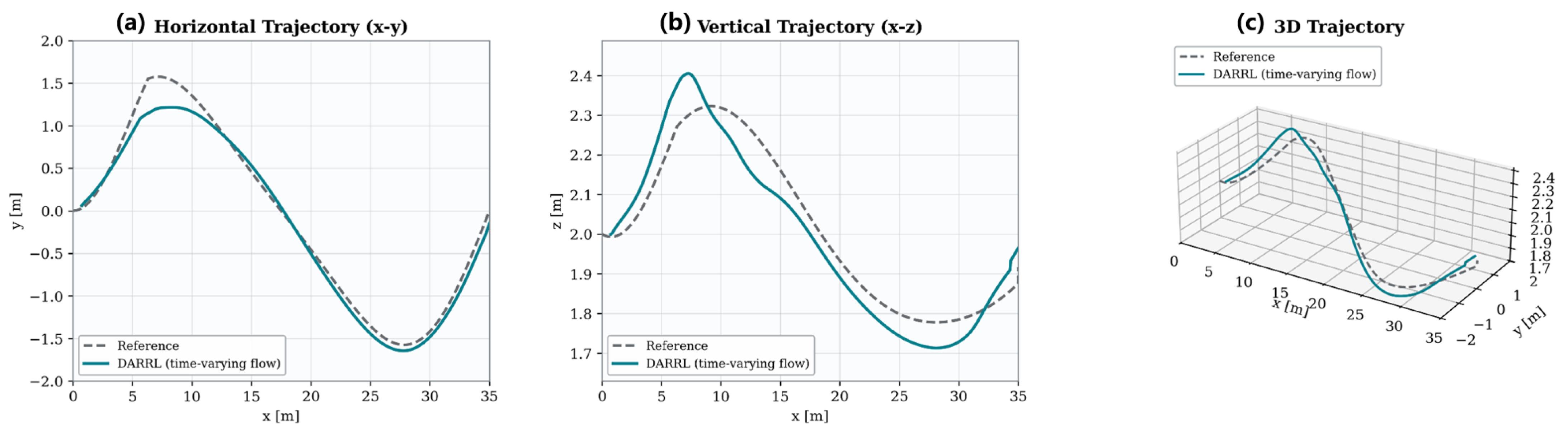
In the Stage-II training environment, the current magnitude and direction are randomly sampled at the beginning of each episode and remain constant throughout the episode. To further evaluate the temporal generalization capability of DARRL under a more complex current condition, the trained policy is directly tested under a time-varying current without any additional training or fine-tuning. The same reference trajectory and initial conditions corresponding to the representative seed 38 in Figure 7 are retained. During the evaluation, the current direction remains fixed, while its magnitude varies according to

$$V_c\left(t\right)=0.3+0.1\sin \left({\displaystyle \frac{2\pi }{20}}t\right),$$

(56)

where $V_c\left(t\right)$ denotes the current speed in $\mathrm{m}/\mathrm{s}$ at time t in seconds. Therefore, the current speed varies sinusoidally between $0.2\mathrm{m}/\mathrm{s}$ and $0.4\mathrm{m}/\mathrm{s}$, with a mean value of $0.3\mathrm{m}/\mathrm{s}$ and a period of $20\mathrm{s}$. Although this magnitude range is consistent with the Stage-II training range, its continuous temporal variation is not included in the training distribution.

As shown in Figure 8, DARRL remains capable of completing the trajectory-tracking task under the time-varying current disturbance. A noticeable deviation occurs around the first curved segment, particularly in the horizontal plane, but the policy subsequently corrects the accumulated error and continues to follow the reference trajectory without divergence. The horizontal and vertical RMSEs are $0.349\mathrm{m}$ and $0.121\mathrm{m}$, respectively, resulting in a 3D RMSE of $0.369\mathrm{m}$. These results demonstrate that DARRL retains effective closed-loop tracking capability under a current condition that changes continuously during execution. They also provide preliminary evidence that the history-based disturbance representation learned by DADE enables the policy to respond to temporal variations in current effects, despite being trained only under episode-wise constant currents.

4.3.3. Component Ablation of DARRL

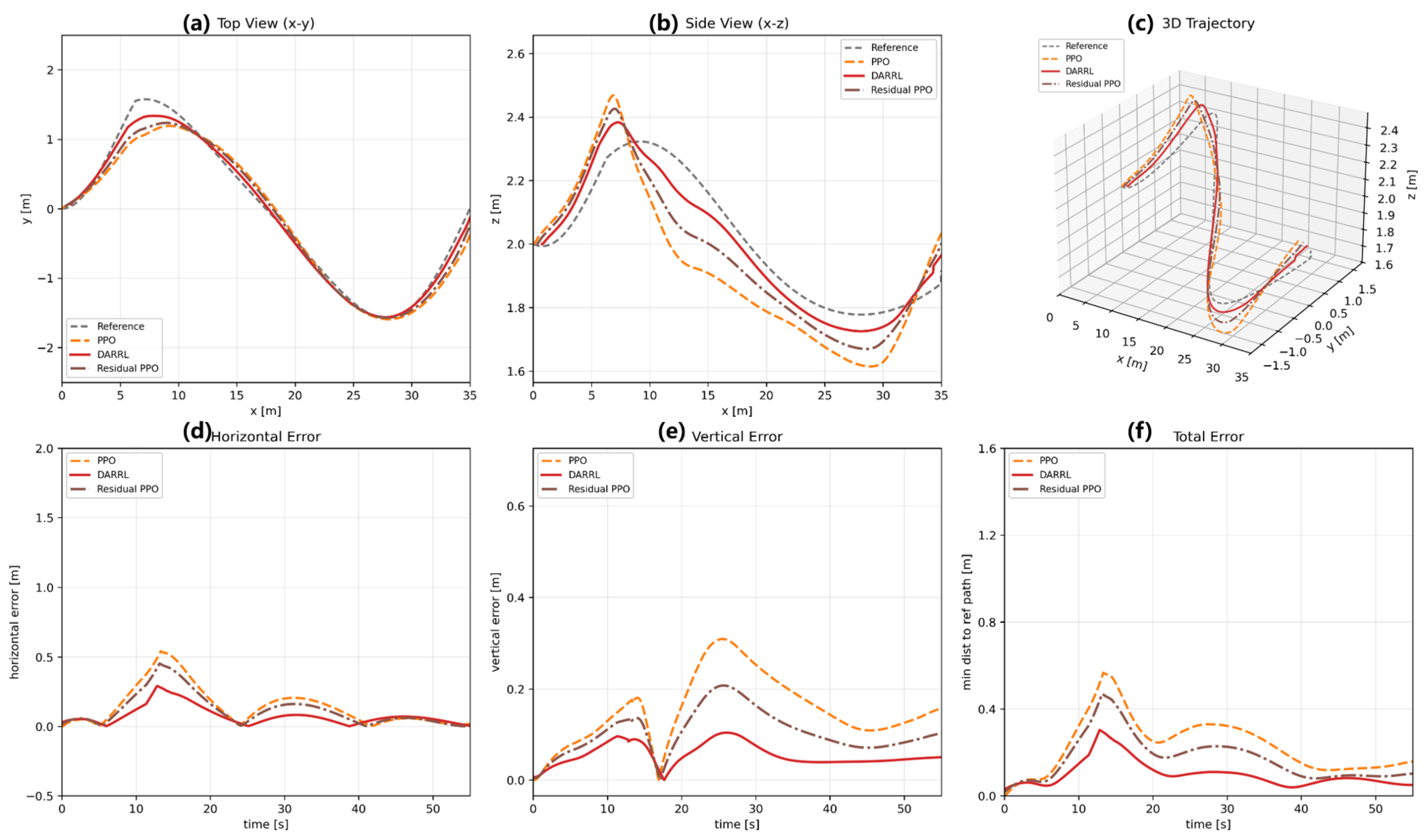
To isolate the respective contributions of residual policy learning and DADE, three configurations are compared: conventional PPO, Residual PPO without DADE, and the complete DARRL. PPO directly optimizes the complete policy without using either the residual policy structure or DADE. Residual PPO retains the frozen MPC-IL base policy and learns only residual action corrections but does not use the historical disturbance representation provided by DADE. The complete DARRL combines residual policy learning with DADE. All configurations use the same environment distribution, policy initialization, training budget, optimization settings, and evaluation protocol. The quantitative results are averaged over 50 independent evaluations with different random seeds, while Figure 9 shows the representative trajectories and tracking errors corresponding to seed 38. As summarized in

Table 5. Component ablation results of DARRL under random current disturbances. The best-performing values are shown in bold.

Method	Residual Learning	DADE	Horizontal Mean Error	Vertical Mean Error	Mean 3D Error	3D RMSE
PPO	No	No	0.228	0.074	0.257	0.436
Residual PPO w/o DADE	Yes	No	0.213	0.071	0.224	0.388
DARRL	Yes	Yes	0.146	0.068	0.175	0.312

, Residual PPO without DADE reduces the horizontal mean error, vertical mean error, mean 3D error, and 3D RMSE by 6.6%, 4.1%, 12.8%, and 11.0%, respectively, compared with conventional PPO. This improvement indicates that restricting reinforcement learning to residual action corrections reduces the policy-optimization difficulty and helps preserve the nominal tracking behavior provided by the MPC-IL policy. Incorporating DADE further improves the tracking performance. Compared with Residual PPO without DADE, DARRL reduces the horizontal mean error, vertical mean error, mean 3D error, and 3D RMSE by 31.5%, 4.2%, 21.9%, and 19.6%, respectively. As shown in Figure 9, Residual PPO generally produces smaller trajectory deviations than PPO, whereas DARRL maintains the lowest and smoothest tracking errors, particularly in segments involving turning maneuvers and current disturbances. The improvement in the vertical mean error is relatively small because Residual PPO already achieves a low vertical error. Nevertheless, the clear reductions in the horizontal error, mean 3D error, and 3D RMSE demonstrate that DADE provides useful historical disturbance information for residual action correction. Overall, these results verify the complementary contributions of residual policy learning and DADE to the complete DARRL framework.

4.3.4. Sensitivity Analysis of the DADE Architecture

To further examine the design choices of DADE, sensitivity analyses are conducted with respect to its temporal-horizon structure and number of attention heads. All variants are trained and evaluated using the same environment distribution, policy architecture, training budget, optimization hyperparameters, and evaluation protocol. Except for the factor being investigated, all other DADE configurations are kept identical to those of the default model. The 3D RMSE is adopted as the evaluation metric because it directly reflects the overall trajectory-tracking performance under current disturbances.

First, the contribution of the dual-horizon structure is evaluated by comparing a short-horizon-only encoder, a long-horizon-only encoder, and the complete dual-horizon encoder. The short-horizon branch uses the most recent 10 observation steps to emphasize the local motion response, whereas the long-horizon branch uses 50 observation steps to capture the accumulated influence of the disturbance over a broader temporal context. The dual-horizon configuration combines these two temporal scales. The corresponding results are reported in

Table 6. Ablation results for different temporal-horizon configurations of DADE. The best-performing values are shown in bold.

Configuration	Short Horizon	Long Horizon	3D RMSE (m)
Short-horizon only	10	–	0.405
Long-horizon only	–	50	0.347
Dual horizon	10	50	0.312

.

As shown in Table 6, the short-horizon-only configuration obtains the highest 3D RMSE of 0.405 m, indicating that a short local history alone is insufficient to represent the accumulated effect of current disturbances on the vehicle motion. Extending the temporal context to 50 steps reduces the RMSE to 0.347 m, showing that the longer-term state evolution provides useful information for disturbance-aware control. Combining the two horizons further reduces the RMSE to 0.312 m. This corresponds to reductions of 23.0% and 10.1% relative to the short-horizon-only and long-horizon-only configurations, respectively. These results indicate that the short- and long-horizon branches provide complementary temporal information: the short branch emphasizes recent motion responses, while the long branch captures broader accumulated trends. Therefore, both branches are retained in the complete DADE architecture.

Second, the sensitivity of DADE to the number of attention heads is investigated. The embedding dimension is fixed at 64 for all variants; consequently, the per-head feature dimensions are 32, 16, and 8 when using two, four, and eight attention heads, respectively. The short- and long-horizon window lengths are fixed at 10 and 50 steps. The results are summarized in

Table 7. Sensitivity of DADE to the number of attention heads. The results are reported as mean ± standard deviation over 20 independent evaluations with different random seeds. The best-performing values are shown in bold.

Configuration	Attention Heads	Dimension per Head	3D RMSE (m)
Dual-H2	2	32	$0.368\pm 0.031$
Dual-H4	4	16	$\mathbf{0}.\mathbf{312}\pm \mathbf{0}.\mathbf{019}$
Dual-H8	8	8	$0.317\pm 0.024$

, where the RMSE values are reported as the mean and standard deviation over 20 independent evaluations with different random seeds.

As shown in Table 7, increasing the number of attention heads from two to four reduces the mean 3D RMSE from 0.368 m to 0.312 m, corresponding to a reduction of 15.2%. This result suggests that two attention heads provide insufficient diversity for representing the temporal dependencies contained in the observation history. Dual-H8 obtains an RMSE of $0.317\pm 0.024$ m, which is close to the $0.312\pm 0.019$ m achieved by Dual-H4. The small difference between these two configurations relative to their observed variability indicates that increasing the number of heads from four to eight does not provide a meaningful additional reduction in tracking error. Moreover, dividing the fixed 64-dimensional embedding into eight heads reduces the dimension of each attention subspace from 16 to 8 and introduces additional head-wise partitioning and implementation overhead without a corresponding performance benefit.

Consequently, the four-head configuration is retained as the default setting because it achieves the lowest mean RMSE while maintaining a balanced representation dimension for each attention head. Overall, the sensitivity results support the use of the dual-horizon structure and show that four attention heads provide an appropriate balance between temporal-representation diversity and per-head representation capacity for the considered disturbance-aware trajectory-tracking task.

4.4. Stage-III Trajectory Execution Under Current Disturbances and Obstacles

4.4.1. Evaluation Protocol and Path-Progress Metric

This section evaluates trajectory execution in the Stage-III environment, which contains both current disturbances and obstacles. In this environment, the goal-reaching rate alone is insufficient to fully characterize the differences among policies. The two key obstacles are located at approximately 12 m and 24 m along the reference path, respectively, resulting in a task with a clear staged difficulty structure. Moreover, an episode may terminate before the robot reaches the goal because of a collision, excessive trajectory or yaw deviation, or the maximum episode length. Therefore, even when a policy fails to reach the goal, the distance traveled along the reference path still provides useful information about its effective execution capability and learning progress.

Accordingly, average path progress is introduced as an additional evaluation metric. Let the path progress achieved in the i-th evaluation episode be

$$P^{\left(i\right)}=\underset{t}{max}\mathcal{S}\left(q_t^{\left(i\right)}\right),$$

(57)

where $q_t^{\left(i\right)}$ denotes the nearest point on the reference trajectory to the robot position at time step t in the i-th episode, and $\mathcal{S}(·)$ denotes the arc-length coordinate along the reference path. The average path progress is then defined as

$$\overline{P}={\displaystyle \frac{1}{N_{\mathrm{eval}}}}{\displaystyle \sum _{i=1}^{N_{\mathrm{eval}}}}{P}^{\left(i\right)},$$

(58)

where $N_{\mathrm{eval}}$ is the number of independent evaluation episodes.

For each initialization strategy and training checkpoint, the quantitative path-progress results are averaged over five repeated evaluations for each of ten evaluation seeds, yielding 50 evaluation episodes in total. The trajectories presented below correspond to one representative evaluation case in which the policies initialized from ${\pi }_0$ and ${\pi }_1$ both reach the goal region. The policy trained from scratch is not included in the representative trajectory comparison because it fails to achieve effective path advancement in most evaluation episodes.

4.4.2. Ablation of Stage-Wise Curriculum Initialization

To isolate the contribution of the proposed stage-wise curriculum, three initialization strategies are compared in the same Stage-III environment. The first policy is trained directly from scratch in the environment with currents and obstacles and therefore receives no prior curriculum. The second policy is initialized from ${\pi }_0$, which inherits the basic trajectory-execution capability learned through MPC-guided imitation learning in Stage I but skips the disturbance-aware training in Stage II. The third policy is initialized from ${\pi }_1$ and follows the complete three-stage curriculum, entering Stage III with both basic trajectory-execution and disturbance-compensation capabilities. Thus, the comparison between ${\pi }_1$ initialization and training from scratch evaluates the overall benefit of curriculum-based policy initialization, whereas the comparison between ${\pi }_1$ and ${\pi }_0$ isolates the contribution of the intermediate disturbance-aware stage.

All three strategies are evaluated at nominal Stage-III training budgets ranging from 100k to 500k frames. To construct a conservative comparison that favors the weaker initialization strategies, the policies initialized from ${\pi }_0$ and from scratch are additionally given 60k and 120k pretraining frames, respectively, in the Stage-III environment. This setting reduces the possibility that the advantage of ${\pi }_1$ initialization is caused merely by unequal opportunities to adapt to the final task.

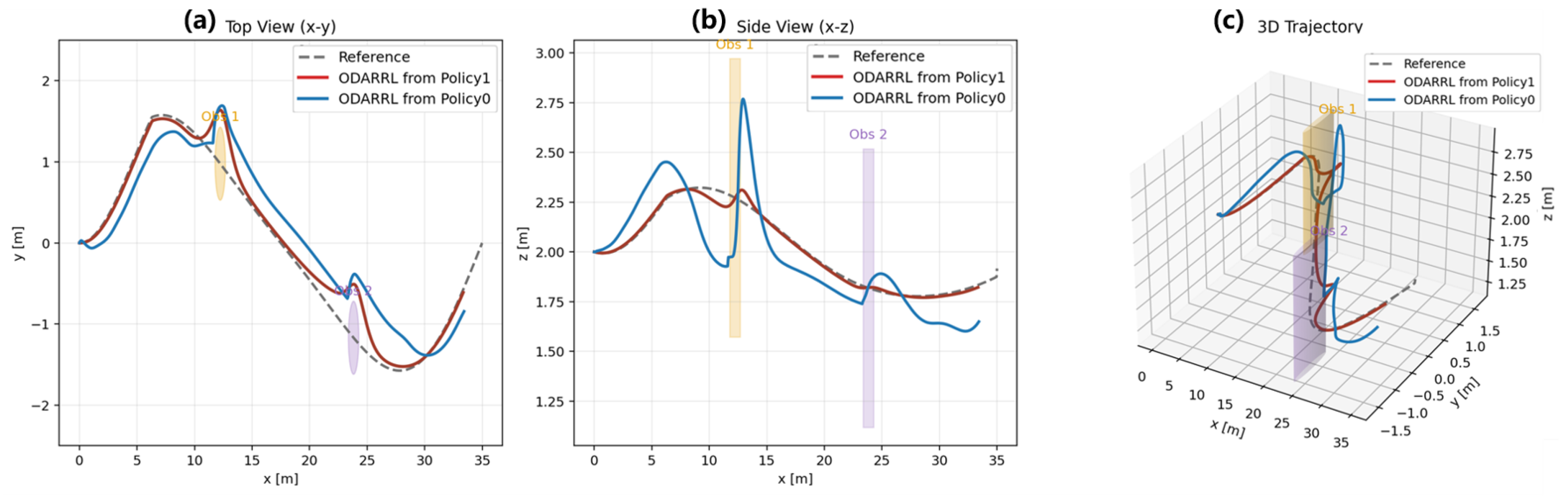
Figure 10 presents representative trajectories for ODARRL initialized from ${\pi }_1$ and ODARRL initialized from ${\pi }_0$. The policy initialized from ${\pi }_1$ follows the reference trajectory more closely in obstacle-free regions and generates smoother, more localized deviations near the obstacles. Around Obs 1, it performs a moderate avoidance maneuver and subsequently returns smoothly toward the reference path. Around Obs 2, it again produces a localized detour while maintaining stable forward progress and recovering toward the reference path after passing the obstacle.

By contrast, the policy initialized from ${\pi }_0$ can avoid the obstacles and advance along the path in the representative case, but it exhibits larger deviations from the reference trajectory, particularly near the obstacle regions. A pronounced vertical excursion is observed around Obs 1, indicating a more abrupt and less coordinated avoidance response. Since ${\pi }_0$ is learned only in the current-free and obstacle-free environment, a policy initialized from ${\pi }_0$ must simultaneously acquire disturbance compensation and obstacle avoidance during Stage III. Consequently, switching into and out of obstacle-avoidance behavior is more likely to degrade its tracking stability under current disturbances. This behavior is reflected in the larger vertical excursion around Obs 1 and the weaker post-avoidance recovery after Obs 2. In comparison, initialization from ${\pi }_1$ results in smoother and more localized trajectory adjustments, suggesting that the disturbance-compensation capability learned in Stage II provides a more favorable prior for obstacle-aware policy learning.

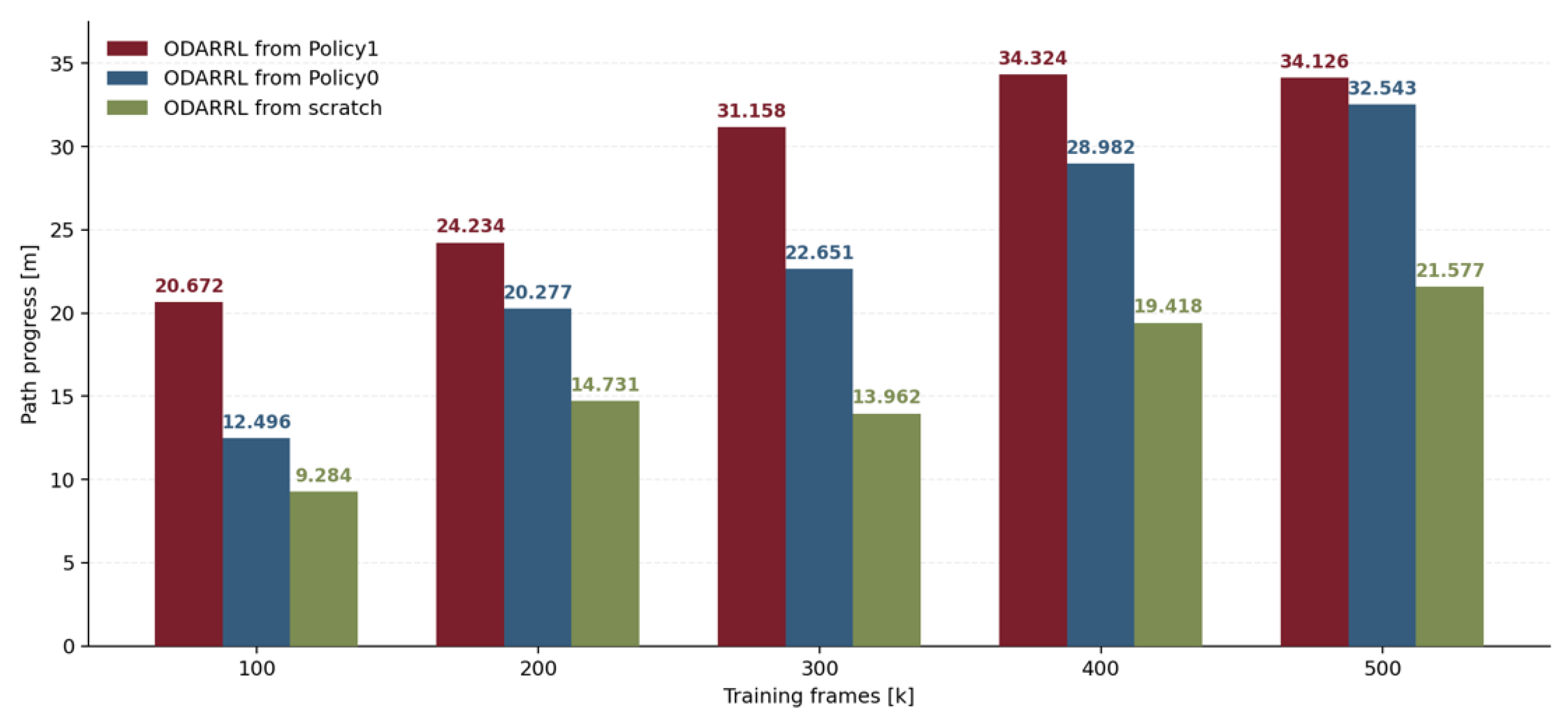
Figure 11 and

Table 8. Performance comparison under different initialization strategies and training budgets in the obstacle-avoidance stage. All values are percentages.

Initialization	Budget	Terminated by Yaw Deviation (%)	Passed at Least One Obstacle (%)	Reached Goal (%)
From scratch	100k	36	0	0
From policy ${\pi }_0$	100k	14	26	0
From policy ${\pi }_1$	100k	0	72	0
From scratch	200k	28	40	0
From policy ${\pi }_0$	200k	4	68	2
From policy ${\pi }_1$	200k	0	92	10
From scratch	300k	26	36	0
From policy ${\pi }_0$	300k	0	74	16
From policy ${\pi }_1$	300k	0	100	72
From scratch	400k	10	68	6
From policy ${\pi }_0$	400k	0	100	46
From policy ${\pi }_1$	400k	0	100	94
From scratch	500k	10	82	10
From policy ${\pi }_0$	500k	0	100	74
From policy ${\pi }_1$	500k	0	100	92

provide quantitative comparisons of the three curriculum-initialization strategies as the Stage-III training budget increases. The policy initialized from ${\pi }_1$ is not terminated by excessive yaw deviation at any of the evaluated checkpoints and consistently achieves the highest path progress and obstacle-passing rate. Its goal-reaching rate increases to 72% at 300k frames and 94% at 400k frames, demonstrating both rapid acquisition of effective obstacle-avoidance behavior and strong final task performance.

The policy initialized from ${\pi }_0$ also improves as training proceeds, but its learning speed and final performance remain inferior to those of the policy initialized from ${\pi }_1$. At 300k frames, the goal-reaching rate of the ${\pi }_0$-initialized policy is only 16%, compared with 72% for the ${\pi }_1$-initialized policy. Even at 500k frames, its goal-reaching rate reaches 74%, whereas the ${\pi }_1$-initialized policy achieves 92%. The policy trained from scratch performs worst overall. It maintains a relatively high yaw-deviation termination rate over a substantial portion of training and reaches a goal-reaching rate of only 10% at 500k frames. These results show that the performance difference is not explained solely by additional exposure to the Stage-III environment, particularly because the weaker initialization strategies are given additional pretraining frames in the conservative comparison.

The observed differences can be explained by the capabilities transferred from the preceding curriculum stages. The policy ${\pi }_0$ primarily learns basic trajectory-execution behavior in a current-free and obstacle-free environment. After entering Stage III, it must therefore adapt simultaneously to the current-compensation requirement and the obstacle-avoidance requirement. This explains why it can advance rapidly to the first obstacle region near 12 m but still struggles to maintain stable behavior afterward. In contrast, the policy ${\pi }_1$ has already acquired disturbance-compensation capability in Stage II. More of its Stage-III learning capacity can consequently be devoted to obstacle avoidance and post-avoidance path recovery instead of relearning current compensation and basic forward progression.

Taken together, the qualitative trajectories in Figure 10, the learning curves in Figure 11, and the quantitative results in Table 8 constitute a stage-wise curriculum ablation. The comparison with training from scratch demonstrates the overall benefit of curriculum-based initialization, the comparison between ${\pi }_0$ and training from scratch demonstrates the value of the Stage-I trajectory-execution prior, and the comparison between ${\pi }_1$ and ${\pi }_0$ demonstrates the additional contribution of the Stage-II disturbance-aware prior. These results show that the complete three-stage curriculum improves both training efficiency and final trajectory-execution performance in environments containing current disturbances and obstacles.

4.5. Discussion

4.5.1. Mechanistic Interpretation of ODARRL

The performance improvement of ODARRL results from the complementary roles of stage-wise curriculum learning, residual policy optimization, and history-based disturbance representation. The three-stage curriculum progressively decomposes the original task into basic trajectory execution, disturbance compensation, and obstacle-aware control. MPC-guided imitation learning first provides a feasible nominal policy, after which the disturbance-aware policy learned in Stage II offers a more suitable initialization for obstacle-aware training. This interpretation is supported by the Stage-III ablation, where initialization from ${\pi }_1$ achieves a goal-reaching rate of 94% at 400k frames, compared with 46% for initialization from ${\pi }_0$ and 6% for training from scratch. Residual learning preserves the basic control behavior of the imitation policy while restricting reinforcement learning to disturbance-induced action corrections. Consequently, the residual actor does not need to relearn the complete thruster-level policy, which reduces the effective optimization difficulty and limits the degradation of previously acquired trajectory-execution capability. Meanwhile, DADE extracts control-relevant disturbance information from observation history to compensate for the limited information available in an instantaneous state. The temporal-horizon ablation shows that combining short- and long-horizon features reduces the 3D RMSE to 0.312 m, compared with 0.405 m and 0.347 m for the corresponding single-horizon variants, confirming the complementary roles of local motion responses and longer-term accumulated effects. Overall, curriculum learning determines how control capabilities are introduced progressively, DADE provides the temporal disturbance context, and residual reinforcement learning converts this information into corrective thruster commands while preserving the nominal policy. Their coordination explains the improved training stability and trajectory-execution performance of the complete ODARRL framework.

4.5.2. Sim-to-Real Considerations and Limitations

Although the proposed method is evaluated using a high-fidelity BlueROV2 Heavy model in Marine Gym, a gap remains between the simulated environment and a physical ROV. In the present study, vehicle-mass randomization is introduced during training to expose the policy to payload variation and model uncertainty. This randomization partially improves robustness to dynamics mismatch; however, it addresses only one source of sim-to-real discrepancy. Other factors, including uncertainties in hydrodynamic coefficients and inertia parameters, thruster dead zones and response delays, sensor noise and state-estimation errors, communication latency, and perception uncertainty, are not fully represented in the current simulation.

Future work will introduce more comprehensive perturbations and uncertainties into the simulation to further evaluate robustness and facilitate sim-to-real transfer. On this basis, the proposed method will be progressively validated and deployed on a physical ROV platform.

5. Conclusions

This paper proposes ODARRL, an obstacle- and disturbance-aware end-to-end residual reinforcement learning framework for safe trajectory execution of underwater robots. To address the challenges posed by random current disturbances, obstacle constraints, and the difficulty of training thruster-level end-to-end control policies in complex underwater environments, a three-stage curriculum learning framework is constructed. First, an initial policy is obtained in a current-free and obstacle-free environment through MPC-guided demonstrations and imitation learning. Second, the robustness of the policy against environmental disturbances is improved through disturbance-aware residual reinforcement learning in random current environments. Finally, the policy is further extended to complex environments involving both currents and obstacles, resulting in a final control policy for safe trajectory execution. Simulation results on the Marine Gym platform with BlueROV2 Heavy demonstrate that the proposed method achieves better trajectory tracking accuracy and robustness under random currents, while also providing higher path progress and more stable training performance in obstacle-involved environments.

Although the effectiveness of the proposed method has been validated in simulation, several directions remain worthy of further investigation. First, the current study mainly focuses on trajectory execution for a single ROV. In future work, the proposed framework can be extended to UVMS scenarios, so that motion control of the vehicle body and disturbance compensation induced by manipulator operation can be learned in a unified framework. Second, the present study is still centered on simulation-based validation. Future work will further investigate the sim-to-real transfer problem, including the influence of perception noise, dynamics mismatch, and environmental uncertainty on policy deployment. Finally, real-world experimental validation will be carried out in subsequent work, including water-tank experiments and open-water sea trials, in order to further assess the feasibility, robustness, and engineering potential of the proposed method in real and complex marine environments.

References

1. Aguirre-Castro, O.A.; Inzunza-González, E.; García-Guerrero, E.E.; Tlelo-Cuautle, E.; López-Bonilla, O.R.; Olguín-Tiznado, J.E.; Cárdenas-Valdez, J.R. Design and Construction of an ROV for Underwater Exploration. Sensors 2019, 19, 5387. [Google Scholar] [CrossRef] [Scilit] [PubMed]
2. Khalid, O.; Hao, G.; Desmond, C.; Macdonald, H.; McAuliffe, F.D.; Dooly, G.; Hu, W. Applications of robotics in floating offshore wind farm operations and maintenance: Literature review and trends. Wind Energy 2022, 25, 1880–1899. [Google Scholar] [CrossRef] [Scilit]
3. Teague, J.; Allen, M.J.; Scott, T.B. The potential of low-cost ROV for use in deep-sea mineral, ore prospecting and monitoring. Ocean Eng. 2018, 147, 333–339. [Google Scholar] [CrossRef] [Scilit]
4. Bingul, Z.; Gul, K. Intelligent-PID with PD feedforward trajectory tracking control of an autonomous underwater vehicle. Machines 2023, 11, 300. [Google Scholar] [CrossRef] [Scilit]
5. Zhang, Y.; Liu, X.; Luo, M.; Yang, C. MPC-based 3-D trajectory tracking for an autonomous underwater vehicle with constraints in complex ocean environments. Ocean Eng. 2019, 189, 106309. [Google Scholar] [CrossRef] [Scilit]
6. Yan, Z.; Wang, M.; Xu, J. Robust adaptive sliding mode control of underactuated autonomous underwater vehicles with uncertain dynamics. Ocean Eng. 2019, 173, 802–809. [Google Scholar] [CrossRef] [Scilit]
7. Tijjani, A.S.; Chemori, A.; Creuze, V. A survey on tracking control of unmanned underwater vehicles: Experiments-based approach. Annu. Rev. Control 2022, 54, 125–147. [Google Scholar] [CrossRef] [Scilit]
8. Hernández-Alvarado, R.; García-Valdovinos, L.G.; Salgado-Jiménez, T.; Gómez-Espinosa, A.; Fonseca-Navarro, F. Neural network-based self-tuning PID control for underwater vehicles. Sensors 2016, 16, 1429. [Google Scholar] [CrossRef] [Scilit] [PubMed]
9. Liang, J.; Huang, W.; Zhou, F.; Liang, J.; Lin, G.; Xiao, E.; Li, H.; Zhang, X. Double-loop PID-type neural network sliding mode control of an uncertain autonomous underwater vehicle model based on a nonlinear high-order observer with unknown disturbance. Mathematics 2022, 10, 3332. [Google Scholar] [CrossRef] [Scilit]
10. Liu, T.; Zhao, J.; Huang, J.; Li, Z.; Xu, L.; Zhao, B. Research on model predictive control of autonomous underwater vehicle based on physics informed neural network modeling. Ocean Eng. 2024, 304, 117844. [Google Scholar] [CrossRef] [Scilit]
11. Eski, İ.; Yildirim, S. Design of neural network control system for controlling trajectory of autonomous underwater vehicles. Int. J. Adv. Robot. Syst. 2014, 11, 7. [Google Scholar] [CrossRef] [Scilit] [PubMed]
12. Yu, T.; Zhang, Q.; Liu, T. Reinforcement learning approaches in the motion systems of autonomous underwater vehicles. Appl. Ocean Res. 2025, 161, 104682. [Google Scholar] [CrossRef] [Scilit]
13. Mirza, K.Z.; Singh, S. Imitation learning for legged robot locomotion: A survey. Front. Robot. AI 2025, 12, 1678567. [Google Scholar] [CrossRef] [Scilit] [PubMed]
14. Vítor, G.d.A.; Melo, D.C.; Maximo, M.R.; Afonso, R.J. Imitation learning of a model predictive controller for real-time humanoid robot walking. Eng. Appl. Artif. Intell. 2025, 143, 109919. [Google Scholar] [CrossRef] [Scilit]
15. Zhou, J.; Mei, J.; Zhao, F.; Chen, J.; Li, S. Online Motion Planning for Quadrotor Multi-Point Navigation Using Efficient Imitation Learning-Based Strategy. In Proceedings of the 2025 IEEE/RSJ International Conference on Intelligent Robots and Systems (IROS); IEEE: New York, NY, USA, 2025; pp. 5386–5393. [Google Scholar]
16. Chrysomallis, I.; Chalkiadakis, G. Imitation Learning in the Deep Learning Era: A Novel Taxonomy and Recent Advances. arXiv 2025, arXiv:2511.03565. [Google Scholar]
17. Tang, C.; Abbatematteo, B.; Hu, J.; Chandra, R.; Martín-Martín, R.; Stone, P. Deep reinforcement learning for robotics: A survey of real-world successes. Annu. Rev. Control Robot. Auton. Syst. 2025, 8, 153–188. [Google Scholar] [CrossRef] [Scilit]
18. Kaufmann, E.; Bauersfeld, L.; Loquercio, A.; Müller, M.; Koltun, V.; Scaramuzza, D. Champion-level drone racing using deep reinforcement learning. Nature 2023, 620, 982–987. [Google Scholar] [CrossRef] [Scilit] [PubMed]
19. Hadi, B.; Khosravi, A.; Sarhadi, P. Deep reinforcement learning for adaptive path planning and control of an autonomous underwater vehicle. Appl. Ocean Res. 2022, 129, 103326. [Google Scholar] [CrossRef] [Scilit]
20. Deowan, M.E.; Yousha, M.S.Y.; Hossain, T.M.; Hassan, S.; Marxer, R. Optimizing Underwater Robot Navigation: A Study of DRL Algorithms and Multi-Modal Sensor Fusion. In Proceedings of the 2025 IEEE International Conference on Robotics and Automation (ICRA); IEEE: New York, NY, USA, 2025; pp. 11270–11277. [Google Scholar]
21. Wu, D.; Feng, Z.; Hou, D.; Liu, R.; Yin, Y. DRL-based path planning and obstacle avoidance of autonomous underwater vehicle. In Proceedings of the 2023 IEEE International Conference on Mechatronics and Automation (ICMA); IEEE: New York, NY, USA, 2023; pp. 948–953. [Google Scholar]
22. Xing, J.; Romero, A.; Bauersfeld, L.; Scaramuzza, D. Bootstrapping reinforcement learning with imitation for vision-based agile flight. arXiv 2024, arXiv:2403.12203. [Google Scholar]
23. Lu, Y.; Fu, J.; Tucker, G.; Pan, X.; Bronstein, E.; Roelofs, R.; Sapp, B.; White, B.; Faust, A.; Whiteson, S.; et al. Imitation is not enough: Robustifying imitation with reinforcement learning for challenging driving scenarios. In Proceedings of the 2023 IEEE/RSJ International Conference on Intelligent Robots and Systems (IROS); IEEE: New York, NY, USA, 2023; pp. 7553–7560. [Google Scholar]
24. Zhang, Y.; Zhang, T.; Li, Y.; Zhuang, Y.; Wang, D. A novel reward-shaping-based soft actor–critic for random trajectory tracking of AUVs. Ocean Eng. 2025, 322, 120505. [Google Scholar] [CrossRef] [Scilit]
25. Niu, S.; Pan, X.; Wang, J.; Li, G. Deep reinforcement learning from human preferences for ROV path tracking. Ocean Eng. 2025, 317, 120036. [Google Scholar] [CrossRef] [Scilit]
26. Lyu, X.; Sun, Y.; Wang, L.; Tan, J.; Zhang, L. End-to-end AUV local motion planning method based on deep reinforcement learning. J. Mar. Sci. Eng. 2023, 11, 1796. [Google Scholar] [CrossRef] [Scilit]
27. Tong, R.; Feng, Y.; Wang, J.; Wu, Z.; Tan, M.; Yu, J. A survey on reinforcement learning methods in bionic underwater robots. Biomimetics 2023, 8, 168. [Google Scholar] [CrossRef] [Scilit] [PubMed]
28. Gao, W.; Zhang, T.; Li, Y.; Zhuang, Y.; Zhang, Y. FRRS-SAC: A deep reinforcement learning framework for three-dimensional AUV docking under ocean disturbances. Ocean Eng. 2026, 357, 125409. [Google Scholar] [CrossRef] [Scilit]
29. Gunnarson, P.; Mandralis, I.; Novati, G.; Koumoutsakos, P.; Dabiri, J.O. Learning efficient navigation in vortical flow fields. Nat. Commun. 2021, 12, 7143. [Google Scholar] [CrossRef] [Scilit] [PubMed]
30. Yao, Q.; Meng, L.; Zhang, Q.; Zhao, J.; Pajarinen, J.; Wang, X.; Li, Z.; Wang, C. Learning-based propulsion control for amphibious quadruped robots with dynamic adaptation to changing environment. IEEE Robot. Autom. Lett. 2023, 8, 7889–7896. [Google Scholar] [CrossRef] [Scilit]
31. Chu, S.; Feng, H.; Ou, Y.; Lin, M.; Li, D. FINDER: Flow-aware intelligent navigation through distilled experience and reinforcement learning for UUVs in complex flow fields. Ocean Eng. 2026, 343, 123188. [Google Scholar] [CrossRef] [Scilit]
32. Chu, S.; Huang, Z.; Li, Y.; Lin, M.; Li, D.; Carlucho, I.; Petillot, Y.R.; Yang, C. MarineGym: A high-performance reinforcement learning platform for underwater robotics. In Proceedings of the 2025 IEEE/RSJ International Conference on Intelligent Robots and Systems (IROS); IEEE: New York, NY, USA, 2025; pp. 17146–17153. [Google Scholar]
33. Fossen, T.I. Nonlinear Modelling and Control of Underwater Vehicles. Ph.D. Thesis, Norwegian Institute of Technology, Trondheim, Norway, 1991. [Google Scholar]
34. Vaswani, A.; Shazeer, N.; Parmar, N.; Uszkoreit, J.; Jones, L.; Gomez, A.N.; Kaiser, Ł.; Polosukhin, I. Attention is all you need. Adv. Neural Inf. Process. Syst. 2017, 30, 5998–6008. [Google Scholar]
35. Schulman, J.; Wolski, F.; Dhariwal, P.; Radford, A.; Klimov, O. Proximal policy optimization algorithms. arXiv 2017, arXiv:1707.06347. [Google Scholar]
36. Chang, S.R.; Huh, U.Y. Curvature-continuous 3d path-planning using qpmi method. Int. J. Adv. Robot. Syst. 2015, 12, 76. [Google Scholar] [CrossRef] [Scilit] [PubMed]
Figure 1. The body frame and the world frame of the BlueROV2 Heavy model.
Jmse 14 01501 g001
Figure 2. A reinforcement learning agent interacting with the environment.
Jmse 14 01501 g002
Figure 3. Overall three-stage curriculum learning framework of the proposed ODARRL method. The policy is first initialized by imitation learning from MPC demonstrations in a current-free environment, then refined in current-disturbed environments, and finally extended to current environments with obstacles to obtain the final obstacle- and disturbance-aware policy.The red arrows indicate ocean-current disturbances.
Jmse 14 01501 g003
Figure 4. Structure of the proposed Dual-Horizon Attention Disturbance Encoder (DADE). Historical observations are divided into a long-horizon window and a short-horizon window, which are processed separately to capture long-term disturbance trends and short-term transient changes. Their outputs are fused by an MLP to generate the disturbance-aware representation.
Jmse 14 01501 g004
Figure 5. Overall architecture of the proposed Disturbance-Aware Residual Reinforcement Learning (DARRL) framework.
Jmse 14 01501 g005
Figure 6. Trajectory tracking comparison between the MPC controller and the imitation-initialized policy π 0 in the current-free environment: (a) top view; (b) side view; (c) 3D trajectory; (d) horizontal error; (e) vertical error; and (f) total error.
Jmse 14 01501 g006
Figure 7. Trajectory tracking comparison among different control methods in the current-disturbed environment: (a) top view; (b) side view; (c) 3D trajectory; (d) horizontal tracking error; (e) vertical tracking error; and (f) total tracking error.
Jmse 14 01501 g007
Figure 8. Trajectory-tracking performance of DARRL under time-varying current disturbances using the representative seed 38: (a) top view; (b) side view; and (c) 3D trajectory.
Jmse 14 01501 g008
Figure 9. Component ablation comparison among different control methods in the current-disturbed environment: (a) top view; (b) side view; (c) 3D trajectory; (d) horizontal tracking error; (e) vertical tracking error; and (f) total tracking error.
Jmse 14 01501 g009
Figure 10. Trajectory comparison among different initialization strategies in the current-disturbed environment with obstacles: (a) top view; (b) side view; and (c) 3D trajectory.
Jmse 14 01501 g010
Figure 11. Average path progress versus training frames for different initialization strategies in the obstacle-involved environment.
Jmse 14 01501 g011