AIS-Based Vessel Trajectory Prediction Using H3-Indexed Historical Trajectory Context

Abstract

Deep learning-based vessel trajectory prediction using Automatic Identification System (AIS) has become a hot topic in the fields of maritime traffic monitoring, situational awareness, and navigational decision support. However, most previous studies have focused primarily on end-to-end model training using trajectory data from a single water area, which limits the resulting models’ ability to generalize to regions with different traffic patterns. To address this issue, this study proposes a method that constructs traffic context from historical AIS records at multiple geographic resolutions using H3, a hexagonal hierarchical spatial indexing system, and integrates this context with a Transformer-based trajectory predictor. A reliability-aware selector determines the contribution of the context to the final prediction, conditioning this decision on the vessel’s motion state and the retrieved historical patterns. Experiments on AIS data from three distinct water areas demonstrated that H3-indexed context improved cross-water prediction accuracy without requiring model retraining on the target area. These findings demonstrate that H3-indexed context, structured at multiple geographic resolutions and integrated through a selective mechanism, serves as transferable spatial context for vessel trajectory prediction.

1. Introduction

Maritime transportation is a key enabler of global trade, facilitating the movement of goods across oceanic, sea, and inland waterways. Vessel trajectory prediction, which is the task of forecasting the future positions of ships based on their past and current movement data such as location, speed, and heading, is essential for maritime traffic situational awareness, collision risk assessment, and navigational decision support. It can be applied to short-term predictions (e.g., the next several minutes) or long-term forecasts (e.g., hours ahead). Given the increasing complexity of maritime operations, the Automatic Identification System (AIS), which provides a continuous record of vessel positions, speeds, and courses at large scale, has become a foundation of maritime research and operational planning.

Vessel trajectory prediction is a complex task influenced by a multitude of factors, including environmental conditions, traffic regulations, vessel interactions, and local operational patterns. Traditional approaches, such as kinematic models and statistical methods, often fail to capture the intricate spatiotemporal dependencies that govern vessel movement over extended horizons. Deep learning architectures have demonstrated significant potential in modeling these dependencies, with approaches ranging from recurrent and attention-based models to more recent Transformer, state-space, and graph-based methods progressively improving the extraction of predictive patterns from AIS data [1,2]. Most existing studies, however, adopt an end-to-end paradigm in which models are trained to map an observed trajectory window directly to future positions. These models often perform well on the training data distribution but exhibit limited generalization to unseen traffic conditions and water areas. Recent studies have explored incorporating richer domain knowledge into trajectory prediction to improve generalization beyond the training distribution. Graph-based methods construct dynamic interaction graphs from contemporaneous vessel observations to capture multi-agent spatial dependencies; retrieval- and memory-augmented methods condition prediction on similar historical trajectory instances stored in external memory; map-aware methods encode navigable geometry and lane topology from vectorized annotations; and learned spatial-memory methods associate grid cells with trainable scene representations that capture local motion regularities. These approaches have demonstrated that trajectory prediction benefits from contextual information beyond the target vessel’s own motion history. However, the spatial knowledge they encode is typically bound to the training region’s learned parameters or requires region-specific resources that limit deployment to new areas without retraining or adaptation.

This paper proposes a method for vessel trajectory prediction that extracts structured traffic patterns from historical AIS records using H3, a hexagonal hierarchical spatial indexing system [3], and validates the approach on real-world data across multiple water areas. The main contributions of this work are as follows:

• We proposed a Transformer-based trajectory prediction model that incorporates historical traffic patterns as contextual information, enabling generalization beyond the training water area.
• We designed an H3-indexed extraction method that constructs structured context from historical AIS records, aggregating trajectory statistics at multiple geographic scales to capture recurring movement patterns.
• We conducted comparative experiments on real-world AIS data from multiple water areas, demonstrating improved prediction accuracy across water areas.

The remainder of this paper is organized as follows. Section 2 reviews the literature on AIS-based vessel trajectory prediction, context-aware methods, and spatial indexing. Section 3 presents the proposed vessel trajectory prediction method, including H3-indexed historical trajectory context construction and the Transformer-based prediction architecture. Section 4 presents the experimental setup, results, and discussion. Section 5 concludes with a summary and directions for future research.

2. Related Work

AIS-based vessel trajectory prediction has progressed through several methodological stages. Early approaches relied on physical motion models, including Kalman filters and particle filters, which extrapolate future positions from kinematic equations without learning from historical trajectory data [4,5]. Subsequent statistical and classical machine learning methods—such as Gaussian process regression, support vector regression, and random forests—introduced data-driven forecasting but were limited by their dependence on hand-crafted features and linear or stationary assumptions that struggled with the nonlinear temporal dynamics of vessel movement [6,7,8,9]. These methods established the feasibility of AIS-based prediction and highlighted the need for architectures capable of learning complex spatiotemporal dependencies directly from data, motivating the shift toward deep learning [1,2].

Deep learning methods have progressively improved the modeling of vessel trajectory dynamics. Recurrent architectures, including long short-term memory (LSTM), bidirectional LSTM (BiLSTM), gated recurrent unit (GRU), and attention-augmented variants such as MHA-BiGRU and TTCN-Attention-GRU, have served as strong baselines for capturing temporal dependencies in vessel trajectories [10,11]. Modern backbones increasingly target longer dependencies and interaction-aware structure. Jiang et al. proposed TRFM-LS, a Transformer-based method for vessel trajectory prediction [12], and Nguyen and Fablet proposed TrAISformer, which models trajectory prediction as a classification task over discretized AIS representations [13]. Subsequent Transformer-based models combine these architectures with generative modeling or long-term forecasting: Wang et al. proposed SocialVAE, which integrates a social variational autoencoder with a Transformer for prediction in complex waterways [14]; Xiong et al. employed the Informer model for long-term ship trajectory prediction [15]; and Yu et al. proposed AISFormer for long-term vessel trajectory prediction [16]. State-space predictors extend this line: Suo et al. introduced the Mamba model for ship trajectory prediction [17], and Xiong et al. proposed MKAIS, which combines Mamba with Kolmogorov-Arnold networks [18]. Graph and diffusion-based methods address interaction structure and multimodal uncertainty more explicitly [19,20,21,22]. These studies strengthen the prediction backbone but rely primarily on the target vessel’s own motion history and do not incorporate historical traffic patterns as contextual information for prediction.

Beyond backbone architecture advances, a growing line of work has explored whether trajectory prediction can benefit from contextual information beyond the observed motion sequence. Several studies employ large language models (LLMs) to incorporate semantic context, navigation intent, and domain knowledge into trajectory prediction: Chen et al. proposed SEMINT, which uses LLM-derived semantic and intent context for long-term prediction [23]; Zhang et al. proposed DI-MTP, which unifies multimodal inputs with explainable navigation intention [24]; and Yu et al. proposed MAKER, a multi-modal knowledge-enhanced framework that learns from trajectory records and textual prompts [25]. Others adapt LLMs to process trajectory data more directly: Jiao et al. proposed LLM4STP, which fuses AIS features through language-model-style representations [26]; Teng et al. proposed STPredictor, which aligns trajectory data with LLM instructions [27]; and Jiao et al. proposed GPT4STP, which adapts pre-trained language models through patching and instance normalization [28]. Most recently, Zhan et al. proposed ShipTraj-R1, which applies reinforcement learning with chain-of-thought reasoning to guide LLM-based ship trajectory prediction [29]. Beyond semantic and textual context, other studies have explored structurally different forms of spatial knowledge. Graph-based maritime models [30,31,32] construct dynamic interaction graphs from contemporaneous vessel observations and propagate information through message passing to capture multi-agent spatial dependencies. Retrieval- and memory-augmented predictors [33,34,35] condition prediction on individual or representative past–future trajectory instances stored in external memory. Map-aware methods [36,37,38] encode navigable geometry and lane connectivity from vectorized annotations to provide structural priors for motion forecasting. Learned spatial-memory methods [39,40,41] associate grid cells with trainable recurrent states or scene embeddings that capture local motion regularities. These methods collectively demonstrate that trajectory prediction benefits from contextual information beyond the target vessel’s own motion history. The context they introduce, however, is either predominantly semantic or textual—derived from language model representations, navigation intent labels, or structured knowledge prompts—or encoded as trainable parameters and region-specific resources (interaction graphs, trajectory databases, vectorized maps, or scene-bound embeddings) that are tied to the training region and limit deployment to new areas without retraining or adaptation.

Large-scale geospatial analysis often requires continuous coordinate space to be converted into discrete spatial units that can be indexed, aggregated, compared, and queried at multiple resolutions. Discrete global grid systems (DGGSs) provide such a framework by partitioning the Earth’s surface into globally addressable cells with a hierarchical spatial structure [42]. H3 is an open-source DGGS implementation based on hierarchical hexagonal cells, offering stable spatial identifiers and compact neighbor queries under a single indexing system [3]. Maritime studies have used hexagonal abstraction to organize spatial information and vessel movement structure [43]. Drapier et al. proposed H3-CLM, which encodes vessel positions as H3 resolution-10 cell identifiers, tokenizes these identifiers into character-level sequences, and trains a Mixtral 220M causal language model to predict future H3 cell sequences from historical AIS data [44]. Legras et al. introduced KH3, which combines H3 cell encoding with discretized speed states and movement-stop flags for compact trajectory indexing and efficient retrieval [45]. Spiliopoulos et al. developed Patterns of Life, a global inventory that aggregates AIS mobility statistics—including course, speed, and cell-to-cell transitions—over 7.3 million H3 hexagonal cells at resolutions 6 and 7, demonstrating the use of H3 as a grid-based maritime traffic statistics framework [46]. Troupiotis-Kapeliaris et al. employed H3-based traffic graphs for dynamic weather-resilient vessel routing [47]; Lee et al. applied H3-grid reinforcement learning to vessel route planning [48]; and Duka et al. used H3 for fishing ground identification from AIS data [49]. These methods treat H3 primarily as a data-management, indexing, or discrete-classification tool, with Patterns of Life as a notable exception that performs per-cell statistical aggregation. Spadon et al. proposed a multi-path forecasting framework that fuses probabilistic route and destination features extracted from historical AIS data with learned trajectory representations for long-term vessel prediction [50]. Despite these advances, no prior work has investigated the systematic use of H3-indexed traffic statistics as a structured, routable context signal for cross-water-area trajectory prediction.

To effectively combine spatial knowledge derived from historical trajectories with deep learning models for vessel trajectory prediction, this study proposes a method based on multi-resolution H3-indexed historical traffic context and a Transformer-based predictor. The method is evaluated on AIS data from multiple water areas, where the addition of H3-indexed context yields consistent improvement in geographic transfer settings.

3. Materials and Methods

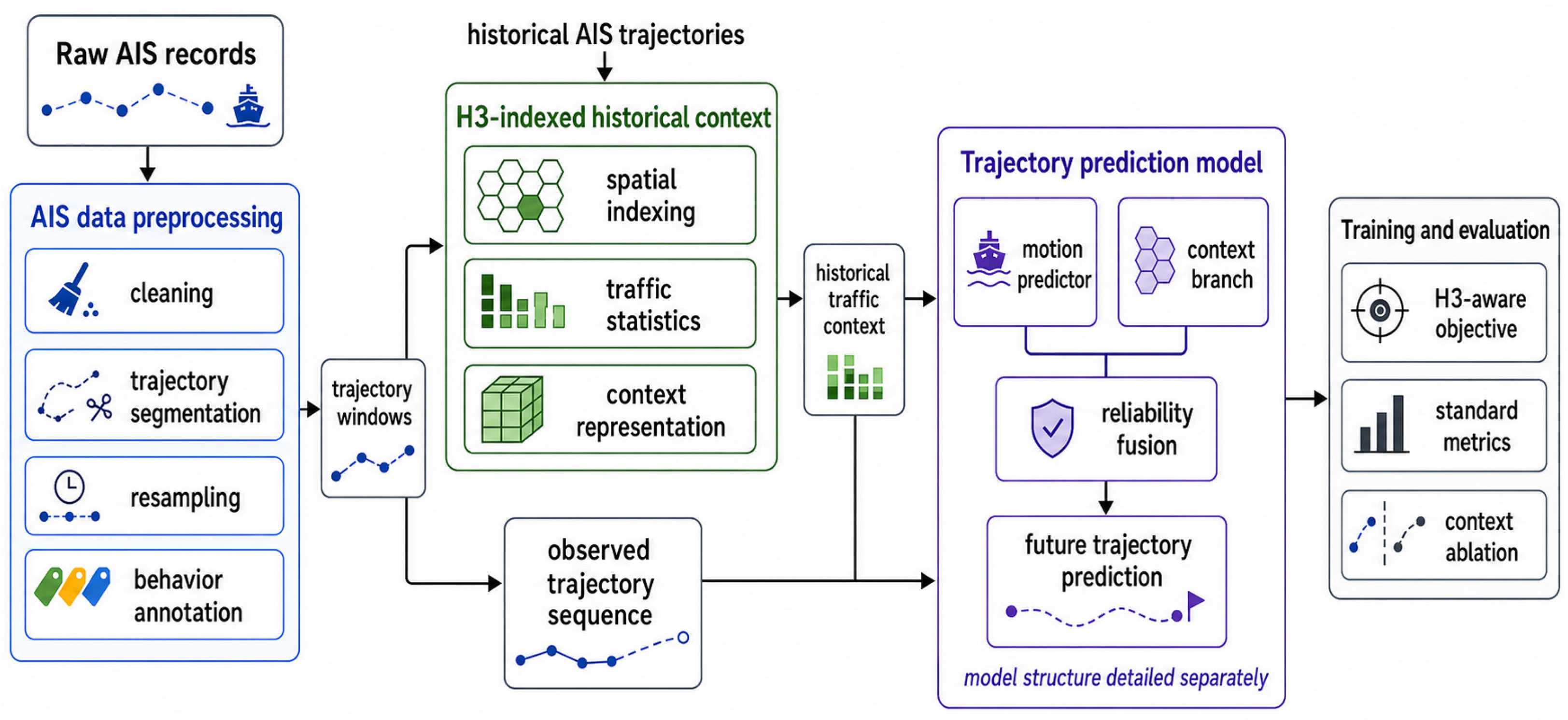
This section describes the methodological workflow of the proposed study. As summarized in Figure 1, raw AIS records are first converted into fixed-length trajectory windows through preprocessing. These windows support two complementary information streams: observed trajectory sequences used by the prediction model, and historical AIS trajectories aggregated into H3-indexed traffic context. The following subsections describe the preprocessing procedure, H3-indexed context construction, trajectory prediction architecture, and training objective and evaluation metrics in sequence.

3.1. AIS Data Preprocessing

AIS provides multidimensional vessel information including Maritime Mobile Service Identity (MMSI), geographic coordinates (latitude and longitude), speed over ground (SOG), course over ground (COG), and timestamp. Raw AIS messages are irregular in time, uneven in vessel density, and may contain incomplete, duplicate, or erroneous records. Thus, before feeding AIS data into the model, the following preprocessing steps are performed, organized from record-level filtering to dataset-level sequence construction, to produce clean, uniformly sampled trajectory windows suitable for model training and evaluation across multiple water areas.

(a)

Data Cleaning and Filtering

Following established AIS preprocessing practices [51], records with missing or invalid MMSI, position, or timestamps are removed, and duplicate reports from the same vessel at the same timestamp are merged into a single record. Physically implausible position jumps are detected by computing the implied speed between consecutive records; records implying a speed greater than 30 kn, or whose reported SOG exceeds 30 kn, or whose reported-to-implied speed difference exceeds 10 kn, are excluded. Records outside the spatial region of interest (ROI) are also removed. Heading values are confined to $[0^{°},{360}^{°}]$ to conform with standard navigational conventions, where $0^{°}$ corresponds to true north and ${360}^{°}$ completes the circle. These operations remove erroneous and out-of-range records and prepare reliable per-vessel data for subsequent trajectory construction.

(b)

Trajectory Construction and Resampling

AIS messages are generally transmitted at different intervals, and consecutive records from a single vessel may span multiple distinct voyages. Validated records are first grouped by MMSI and sorted by timestamp. To prevent the concatenation of separate voyages into a single sequence, a trajectory is segmented when the time gap between consecutive records exceeds 4 h. Segments shorter than 30 min or with fewer than 50 points are discarded, as they provide insufficient motion context for reliable prediction. Each retained segment is resampled to a uniform 5 min interval via a time-weighted linear interpolation method. Because course over ground is circular, it is decomposed into sine and cosine components before interpolation to avoid discontinuity at the $0^{°}$/${360}^{°}$ boundary. The resulting sequences are temporally aligned, suitable for subsequent behavior annotation and prediction. These thresholds were selected during preliminary development and held fixed across all study areas.

(c)

Behavior Annotation

Following trajectory resampling, a centered moving-average filter is applied to the instantaneous speed to reduce AIS reporting noise. Points are then classified by comparing the filtered speed against two thresholds: a stationary threshold of 2.0 kn and a navigating threshold of 8.0 kn. Low-speed points below the stationary threshold are further examined using trajectory-level indicators, including cumulative path length, net displacement, and the ratio of displacement to path length, to distinguish stationary behavior (anchored vessels whose positions oscillate within a limited radius) from slow local motion (trawling or harbor maneuvering along irregular low-speed paths). Points above the navigating threshold are classified as sailing, and intermediate speeds as maneuvering. Each trajectory point is thereby assigned one of three behavior labels: stationary, maneuvering, or sailing, which is used in subsequent analysis.

(d)

Data Preparation for Model Inputs

To generate model-ready trajectory sequences from the resampled trajectories, a sliding window of fixed observation and prediction lengths is applied across each trajectory segment, extracting fixed-length trajectory sequences. Each sequence consists of an observation window spanning the most recent steps and a prediction target spanning the subsequent steps. The last observed point of each sequence is taken as the local-coordinate origin: geographic coordinates are converted into east–north displacement in meters, and speed and course over ground are decomposed into eastward and northward velocity components, so that each sequence is represented in a self-contained local frame. Each trajectory sequence supplies four input features per step and a displacement target, and serves as the common data unit for the subsequent H3-indexed context construction and trajectory prediction modules. The sequence lengths and scaling constants are specified in the experimental setup.

3.2. H3-Indexed Historical Traffic Context Construction

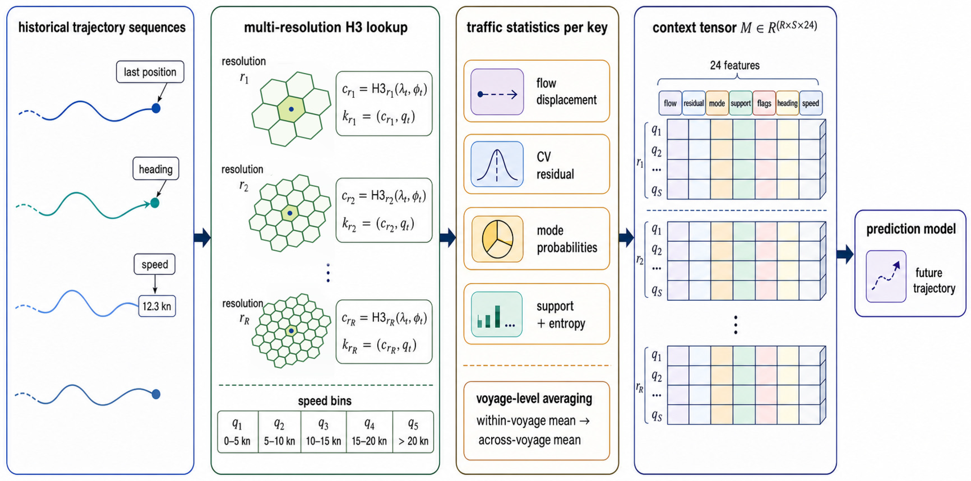
Maritime traffic flow analysis aims to extract spatial knowledge from historical AIS data, including dominant route corridors, traffic density distributions, and typical vessel activity at given locations. Such knowledge is often summarized through aggregate statistics or visual representations, but it is less commonly organized as numerical input features for trajectory prediction. To bridge this gap, we construct H3-indexed context maps that encode these traffic statistics as structured numerical tokens and supply them to the predictor as an independent context branch. Historical trajectory sequences are aggregated at multiple H3 resolutions and organized by H3 cell, discretized heading, and vessel speed, yielding per-location statistics across multiple speed regimes that capture how vessels traveling at different speeds behave at the same location and heading. Figure 2 illustrates this construction.

3.2.1. H3 Spatial Indexing and Multi-Resolution Lookup

To organize historical traffic statistics by geographic location, a spatial indexing system is used to map continuous vessel positions into discrete spatial identifiers at multiple scales. This study adopts the H3 spatial indexing system, which partitions the Earth’s surface into hierarchical hexagonal cells identified by 64-bit integers, offering 16 resolution levels from global to sub-meter [3]. The last observed position of each trajectory sequence is mapped to an H3 cell, and the vessel’s instantaneous heading is discretized to form a combined lookup key:

$$c_r={\mathrm{H}3}_r\left({\lambda }_t,{\varphi }_t\right), k_r=(c_r,q_t),$$

(1)

where $({\lambda }_t,{\varphi }_t)$ denotes the last observed longitude and latitude, and $q_t\in \{0,1,2,3\}$ denotes the heading bin, centered at $0^{°}$, ${90}^{°}$, ${180}^{°}$, and ${270}^{°}$, respectively.

H3 is chosen over axis-aligned rectangular grids or string-based alternatives such as Geohash for several reasons specific to the aggregation of maritime traffic statistics. First, hexagonal cells at each resolution have near-equal area, ensuring that traffic statistics computed per cell are based on comparable spatial units regardless of geographic location—a property not provided in the same way by latitude–longitude grids, Geohash, or Google S2. Second, the uniform six-neighbor structure of hexagons avoids the anisotropic distance artifacts that rectangular grids introduce when computing directional movement statistics. Third, the explicit parent–child hierarchy and built-in neighbor queries allow traffic statistics to be queried at multiple spatial scales while mitigating boundary effects. When a vessel is located at the edge of a cell, statistics from neighboring cells can be incorporated to avoid artifacts caused by arbitrary grid boundaries. The same parent–child relationship also enables context to be queried at progressively coarser resolutions under a single indexing system, without redefining grid boundaries across water areas. H3 offers 16 resolution levels with progressively finer spatial granularity, allowing researchers to select the range that matches the spatial scale of their study area.

3.2.2. Historical Traffic Statistics Aggregation

For each H3 cell $c_r$ and heading bin $q_t$, the H3-indexed context map stores three groups of statistics computed from the historical trajectory sequences whose last observed position falls into $c_r$ and whose heading matches $q_t$: flow and residual displacement, behavior-mode probabilities, and support score and mode-probability entropy.

(a)

Flow and residual displacement

For each spatial key, the final displacement over the prediction horizon is computed in local east–north coordinates. Its mean value captures the dominant movement direction and magnitude historically observed at that location and heading. A constant-velocity extrapolation from the last observed speed and heading is subtracted from this displacement, yielding a residual component that isolates location-specific deviation from inertial motion. To avoid interference from anchored or drifting vessels, stationary voyage segments contribute zero displacement to the flow and residual statistics, effectively excluding their near-zero displacement from the mean.

(b)

Behavior-mode probabilities

The proportions of $\{\mathrm{stationary},\mathrm{maneuvering},\mathrm{sailing}\}$ trajectory sequences, derived from the behavior labels assigned in Section 3.1(c), characterize the typical movement patterns at each spatial key, distinguishing shipping lanes dominated by sailing traffic from anchorage areas and zones of frequent maneuvering.

(c)

Support score and mode-probability entropy

The support score measures the amount of historical trajectory evidence available for each spatial key. It is computed as a smoothed sample-count ratio $n/(n+8)$, where $n$ denotes the number of contributing trajectory sequences. The form $n/(n+k)$ is zero when no evidence is available, increases monotonically, and approaches one only for well-observed keys; the constant $k=8$ sets the half-saturation point, so that a key supported by eight independent voyage contributions receives a score of 0.5. This value is chosen a priori as a leverage threshold: at $n=8$, no single voyage contributes more than 12.5% of the aggregate, preventing individual outliers from dominating the per-cell statistics. The score is not used as a fixed multiplicative weight; rather, it is exposed as a feature to the learned selector (Section 3.3), allowing the model to interpret evidence availability in context. Mode-probability entropy captures the diversity of movement patterns among the contributing trajectory sequences: a shipping lane dominated by sailing traffic receives low entropy, while a multi-use area—such as a port entrance where vessels anchor, maneuver, and transit—receives high entropy. Entropy is computed from the normalized behavior-mode distribution, ranging from 0 when a single mode dominates to 1 when all three modes are equally represented. Together, the support score and entropy characterize the coverage and behavioral composition of the traffic at each spatial key.

Within each $(c_r,q_t)$ key, the contributing trajectory sequences are partitioned by discretized observed speed into five bins (0–1, 1–3, 3–6, 6–10, and above 10 kn). Each speed bin independently yields flow, residual, mode, and support-score statistics, producing one candidate token per bin per resolution. The model receives all speed-bin candidates and uses the observed speed of the query sequence to select or interpolate among them. To prevent correlated trajectory sequences within a voyage from dominating the aggregated statistics, sequences belonging to the same voyage segment are first averaged to produce a single per-voyage contribution before the across-voyage statistics are computed.

3.2.3. Context Token Encoding

With the H3-indexed statistics established for each spatial key and speed bin, the retrieved context is encoded as a 24-dimensional token for model input. The token contains seven field groups: flow displacement, constant-velocity residual, behavior-mode probabilities, support score and mode-probability entropy, lookup-status flags, heading features, and speed-bin identifiers.

Repeating this process at multiple H3 resolutions yields a set of per-resolution, per-speed-bin candidate tokens. These are organized into a context tensor $M\in {\mathbb{R}}^{R\times S\times 24}$, where $R$ and $S$ denote the number of H3 resolutions and speed bins, respectively. The model receives all candidates and uses the observed speed of the query sequence to select or interpolate among them, as described in Section 3.3. The dimensional allocation and definitions of these seven field groups are summarized in

Table 1. H3-indexed context token layout.

Field	Dim	Description
Flow displacement	2	Mean east/north displacement over the prediction horizon, averaged from historical trajectory sequences at the matched H3 key.
Constant-velocity (CV) residual	2	Residual displacement after subtracting a constant-velocity extrapolation from the flow displacement.
Mode probabilities	3	Proportions of stationary, maneuvering, and sailing labels among the contributing trajectory sequences.
Support score and entropy	2	Smoothed support score from the trajectory-sequence count; mode-probability entropy from the behavior-mode distribution.
Lookup flags	5	One-hot indicators: exact-speed, cell-speed-fallback, heading-fallback, cell-fallback, or no-map.
Heading features	4	Sine and cosine of the current heading and the discretized heading-bin center.
Speed identifiers	6	One-hot encoding of the speed bin and the bin-center speed value.

.

Each field group serves a specific role in characterizing the historical traffic context. Flow displacement and its constant-velocity residual jointly describe the dominant movement pattern at a given location: the flow captures the mean historical displacement, while the residual isolates location-specific deviations from inertial motion, such as curvature or deceleration near a channel bend. Heading-conditioned aggregation ensures that these statistics reflect traffic moving in a direction similar to the query vessel, rather than blending opposing flows. Speed-bin partitioning separates vessels in directed transit from those engaged in local operations, so that the retrieved statistics match the query vessel’s operational mode. The support score and mode-probability entropy provide the selector with an explicit measure of how well-grounded the retrieved statistics are: a cell with few contributing voyages or a diffuse behavior-mode distribution signals lower reliability. Lookup flags inform the selector whether the retrieved token is based on an exact key match or a coarser fallback, and heading and speed identifiers allow the selector to assess the alignment between the query vessel’s state and the token’s conditioning.

3.3. Trajectory Prediction Architecture

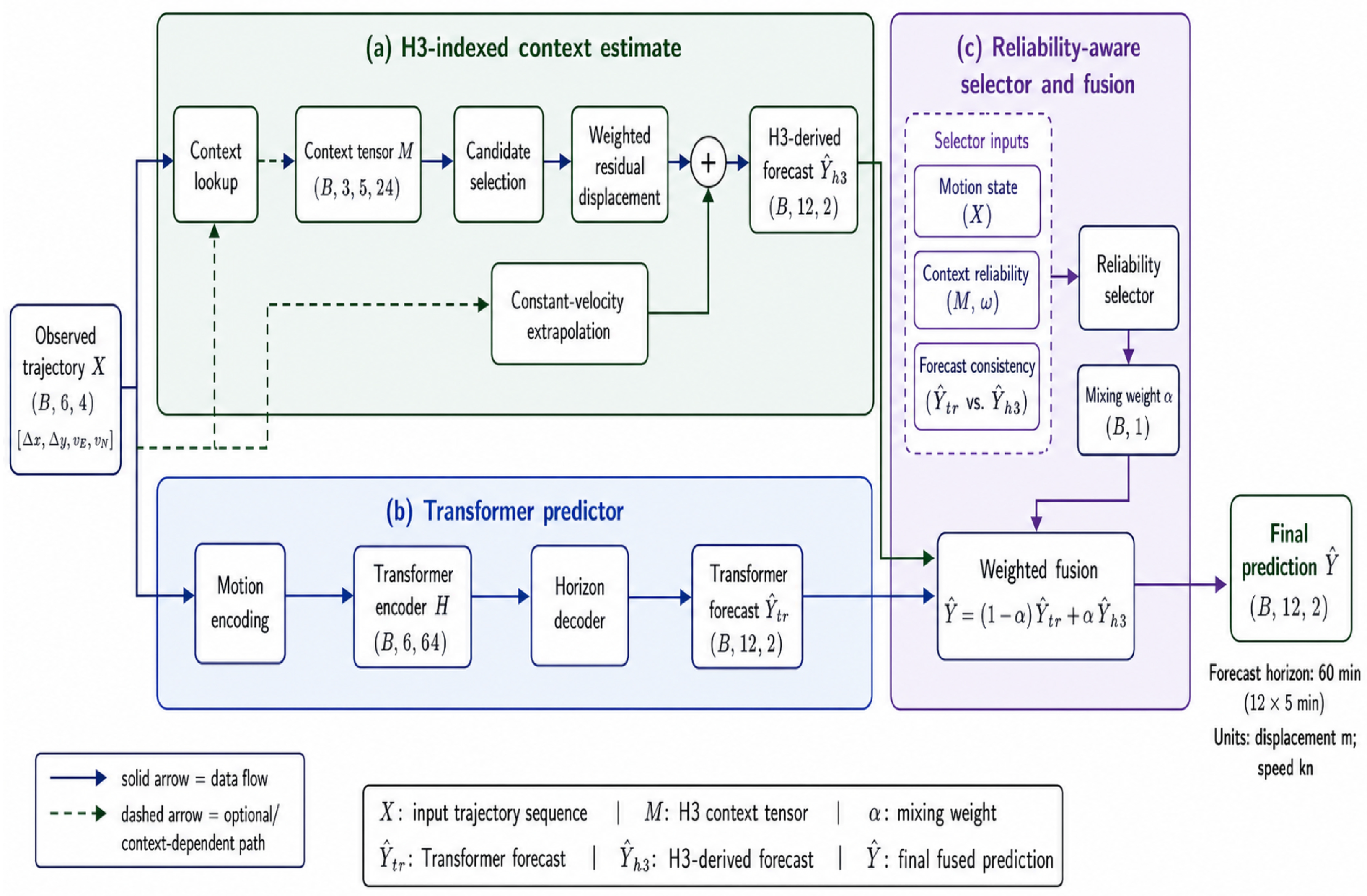
The proposed architecture contains two parallel predictive sources that operate on the objects defined in the preceding sections: a Transformer predictor that forecasts from the vessel’s own observed motion (the trajectory sequence $\mathit{X}$ from Section 3.1), and an H3-indexed context branch that uses $\mathit{X}$ to look up the historical traffic statistics represented by $M$ (Section 3.2.1) and convert them into an H3-derived forecast. A reliability-aware selector combines the two displacement sources into the final prediction. Figure 3 illustrates this prediction architecture, and the following subsections describe the Transformer predictor, the H3-derived forecast, and the selector.

3.3.1. Transformer Predictor

The proposed architecture combines a Transformer predictor with an H3-indexed context component. The Transformer predictor produces the base displacement forecast from the vessel’s own observed motion. The input is the trajectory sequence defined in Section 3.1, organized as

$$\mathit{X}=\left[{\mathit{x}}_1,{\mathit{x}}_2,\dots ,{\mathit{x}}_L\right]\in {\mathbb{R}}^{L\times 4}, {\mathit{x}}_t=[\Delta x_t,\hspace{0.33em}\Delta y_t,\hspace{0.33em}{v}_t^x,\hspace{0.33em}{v}_t^y],$$

(2)

where $\Delta x_t,\Delta y_t$ are the local displacements along the east ($x$) and north ($y$) axes, and $v_t^x,v_t^y$ the corresponding $x$- and $y$-velocity components at step $t$, all defined relative to the last observed point.

The input features are first projected to a latent dimension $d$ through a linear layer and combined with a positional embedding so that the encoder can distinguish the temporal order of the observation steps:

$$\mathit{H}=\mathrm{T}\mathrm{r}\mathrm{a}\mathrm{n}\mathrm{s}\mathrm{f}\mathrm{o}\mathrm{r}\mathrm{m}\mathrm{e}\mathrm{r}\mathrm{E}\mathrm{n}\mathrm{c}\mathrm{o}\mathrm{d}\mathrm{e}\mathrm{r}(W_x\mathit{X}+E_{\mathrm{p}\mathrm{o}\mathrm{s}}),$$

(3)

where $W_x\in {\mathbb{R}}^{4\times d}$ projects the four input features and $E_{\mathrm{p}\mathrm{o}\mathrm{s}}\in {\mathbb{R}}^{L\times d}$ is a learned embedding.

The Transformer encoder consists of stacked multi-head self-attention layers. At each layer, every observation step attends to all other steps within the sequence, weighted by their relevance to the current prediction context. This mechanism captures short-term temporal dependencies that are essential for trajectory forecasting, including changes in speed, turning behavior, and acceleration or deceleration patterns.

The encoder output $\mathit{H}$ is flattened into a single context vector and passed through a multilayer perceptron (MLP) horizon decoder:

$${\widehat{Y}}_{\mathrm{t}\mathrm{r}}=g_{\theta }(\mathrm{v}\mathrm{e}\mathrm{c}(\mathit{H})),$$

(4)

where $g_{\theta }$ is a two-layer MLP with Gaussian error linear unit (GELU) activation and dropout that directly outputs the multi-step displacement forecast ${\widehat{Y}}_{\mathrm{t}\mathrm{r}}\in {\mathbb{R}}^{H\times 2}$. Displacement rather than absolute coordinates is predicted, with the origin reset to the last observed point of each trajectory sequence.

3.3.2. H3-Derived Forecast

While the Transformer predictor forecasts from the vessel’s own motion, it cannot exploit recurring location-specific traffic patterns in a given water area, including typical routes, speed regimes, and common maneuver points. To incorporate this information, the H3-indexed context tensor $M$, constructed in Section 3.2.1, encodes historical traffic statistics as candidate tokens across multiple resolutions and speed bins. From these candidates, the model extracts a traffic-conditioned displacement estimate that complements the base forecast.

A candidate-selection network assigns a weight to each token according to its content, the consistency between the observed vessel speed and the token’s speed-bin center, and the H3 resolution indicator:

$${\omega }_{r,s}={\mathrm{s}\mathrm{o}\mathrm{f}\mathrm{t}\mathrm{m}\mathrm{a}\mathrm{x}}_{r,s}\left(a_{\psi }(m_{r,s},\mathit{X})\right),$$

(5)

where $m_{r,s}$ denotes the token at resolution $r$ and speed bin $s$, and $a_{\psi }$ is a lightweight feed-forward network.

The weighted historical residual is then added to a constant-velocity extrapolation from the last observed state, yielding the H3-derived forecast:

$${\widehat{Y}}_{\mathrm{h}3}={\widehat{Y}}_{\mathrm{C}\mathrm{V}}+{\Delta }_{\mathrm{h}\mathrm{i}\mathrm{s}\mathrm{t}}(\mathit{X},M),$$

(6)

where ${\Delta }_{\mathrm{h}\mathrm{i}\mathrm{s}\mathrm{t}}$ is the weighted sum of the residual displacement fields across the selected candidate tokens, linearly interpolated over the prediction horizon. This H3-derived forecast captures the dominant displacement patterns at the vessel’s location, providing an alternative predictive signal that the selector can draw on when historical context is informative.

3.3.3. Reliability-Aware Selector

The H3-derived forecast is not equally informative for every vessel state. A vessel on a busy shipping lane may follow a stable traffic pattern, whereas a stationary vessel at anchor or a vessel engaged in local maneuvering may deviate from the aggregated historical pattern. Rather than using the H3-derived forecast unconditionally, the reliability-aware selector estimates, for each trajectory sequence, how much weight should be assigned to the Transformer forecast and to the H3-derived forecast.

The routing branch comprises two separate feed-forward networks that operate at different stages of the context integration process.

(a)

Candidate selector.

The first network assigns a weight to each of the $R \times S$ candidate tokens in the context tensor $M$. For each token $m_{r,s}$, the network receives a 31-dimensional input consisting of the 24-dimensional token itself, the current and mean vessel speeds, two speed-center distances measuring the offset between the observed speed and the token’s speed-bin center, and a 3-dimensional one-hot resolution indicator. The network applies layer normalization, a linear projection to 64 hidden units with GELU activation, and a linear output layer producing a scalar logit. A softmax over all $R\times S=15$ candidates yields the selection weights ${\omega }_{r,s}$ (Equation (5)). This network contains 2175 parameters.

(b)

Final reliability gate.

The second network determines the overall mixing coefficient $\alpha$ that governs the convex combination of the Transformer and H3-derived forecasts. Its 20-dimensional input is assembled from three groups: (i) 4 input-state features—logarithmic path length, logarithmic net displacement, current speed, and mean speed over the observation window; (ii) 5 forecast-consistency features—endpoint distances between the Transformer forecast, the H3-derived forecast, and a constant-velocity extrapolation, together with the mean horizon divergence between the Transformer and H3-derived forecasts; and (iii) 11 weighted H3 summary features—the flow norm, residual norm, three mode probabilities, support score, composite reliability, exact-lookup weight, lookup quality, and no-map weight, all computed from the candidate-selected context. The network applies layer normalization, a linear projection to 48 hidden units with GELU activation and dropout (rate 0.1), and a sigmoid output layer, producing ${\alpha }_{\mathrm{b}\mathrm{a}\mathrm{s}\mathrm{e}}\in [0,1]$. This network contains 1097 parameters. Together, the two routing networks add 3272 trainable parameters to the model.

(c)

Speed-conditioned modulation.

The base coefficient ${\alpha }_{\mathrm{b}\mathrm{a}\mathrm{s}\mathrm{e}}$ is further modulated by a speed-conditioned multiplier before entering the final fusion. The H3 context encodes historical traffic-flow patterns—heading distributions, speed regimes, and residual displacement statistics—that characterize how vessels typically transit through a region. These flow statistics are most informative for vessels in directed transit at speed, whose future positions are likely to follow established route patterns. For low-speed vessels engaged in local operations—maneuvering, docking, or anchor swinging—motion is dominated by site-specific activity rather than by regional traffic flow, and a historical flow prior can be misleading. The multiplier therefore attenuates the H3 contribution at low speeds:

$$m\left(v\right)=\left\{\begin{array}{ll}0.20& v <3.0\hspace{0.33em}\mathrm{kn}\\ 0.60& 3.0 \le v <5.0\hspace{0.33em}\mathrm{kn}\\ 1.00& v \ge 5.0\hspace{0.33em}\mathrm{kn}\end{array}\right.$$

(7)

where $v$ is the current vessel speed in knots. A local-motion suppression term $s_{\mathrm{s}\mathrm{u}\mathrm{p}\mathrm{p}\mathrm{r}\mathrm{e}\mathrm{s}\mathrm{s}}\in [0,1]$ further attenuates the gate when the vessel exhibits low-speed, low-displacement behavior, using sigmoid functions of the current speed, net displacement, and cumulative path length over the observation window. The final mixing coefficient is the product of these three factors, clipped to $[0,1]$:

$$\alpha =[\hspace{0.17em}{\alpha }_{\mathrm{b}\mathrm{a}\mathrm{s}\mathrm{e}}\cdot m(v)\cdot s_{\mathrm{s}\mathrm{u}\mathrm{p}\mathrm{p}\mathrm{r}\mathrm{e}\mathrm{s}\mathrm{s}}\hspace{0.17em}{]}_0^1.$$

(8)

In the low-motion regime ($v <3$ kn with negligible displacement), the combined attenuation drives $\alpha$ toward zero, effectively closing the H3 branch regardless of the gate’s raw output. In the high-motion regime ($v \ge 5$ kn with substantial displacement), both $m\left(v\right)$ and $s_{\mathrm{s}\mathrm{u}\mathrm{p}\mathrm{p}\mathrm{r}\mathrm{e}\mathrm{s}\mathrm{s}}$ approach one, and the gate’s decision is preserved.

The final prediction is a convex combination of the two displacement sources:

$$\widehat{Y}=(1-\alpha ){\widehat{Y}}_{\mathrm{t}\mathrm{r}}+\alpha {\widehat{Y}}_{\mathrm{h}3}.$$

(9)

In this way, the selector uses vessel motion, H3-context reliability, and forecast consistency to decide when historical traffic patterns provide a reliable cue and when the Transformer forecast should dominate. The support score and composite reliability in the gate input allow the selector to assess whether the retrieved context is well-grounded: a cell with few contributing voyages or a diffuse behavior-mode distribution produces a low reliability signal, prompting the gate to reduce $\alpha$. This design ensures that the H3 context contributes to the prediction only when the historical evidence is both available and consistent with the vessel’s current motion state.

3.4. Training Objective and Evaluation Metrics

3.4.1. Training Objective

A common training loss for trajectory prediction models is the mean squared error (MSE), which penalizes the Euclidean deviation between predicted and ground-truth displacements at each future step. In AIS-based vessel trajectory datasets, however, this loss can overemphasize stationary or near-stationary samples. Vessels at anchor or under mooring constraints may exhibit small position oscillations caused by local drift, anchor-chain movement, or measurement noise, although they have not made a meaningful trajectory transition. The spatial scale of this oscillation is physically determined by the vessel’s swinging-circle radius—the cable paid out plus the vessel length—which for commercial vessels typically falls in the range of several hundred meters to approximately one kilometer. Penalizing these local deviations in the same way as sailing or maneuvering errors can encourage the model to fit noise-like stationary motion. To reduce this effect, this study uses an H3-aware loss that introduces a spatial tolerance for stationary sequences. The tolerance is defined by H3 grid membership at resolution 8 with a one-ring neighborhood (kring = 1): if the predicted position falls within the ground-truth cell or its six immediate neighbors, the displacement error is treated as zero; otherwise, standard Euclidean error is applied.

Let ${\widehat{\mathit{p}}}_{i,h}$ and ${\mathit{p}}_{i,h}$ be the predicted and ground-truth displacement at step $h$ in the normalized coordinate frame described in Section 3.1, and $\mathcal{S}$ the set of stationary samples. The position component of the H3-aware loss is

$${\mathcal{l}}_{i,h}^{\mathrm{H}3}=\left\{\begin{array}{ll}0,& i\in \mathcal{S}\hspace{0.25em}\mathrm{and}\hspace{0.25em}\parallel {\widehat{\mathit{p}}}_{i,h}-{\mathit{p}}_{i,h}\parallel \le \rho ,\\ \parallel {\widehat{\mathit{p}}}_{i,h}-{\mathit{p}}_{i,h}{\parallel }^2,& \mathrm{otherwise},\end{array}\right.$$

(10)

where $\rho$ is the H3 one-ring neighborhood tolerance. For maneuvering and sailing sequences, ${\mathcal{l}}_{i,h}^{\mathrm{H}3}=\parallel {\widehat{\mathit{p}}}_{i,h}-{\mathit{p}}_{i,h}{\parallel }^2$. Velocity components are always evaluated with standard MSE; the H3 tolerance affects only the position component for stationary samples. Both the Transformer forecast ${\widehat{Y}}_{\mathrm{t}\mathrm{r}}$ and the H3-derived forecast ${\widehat{Y}}_{\mathrm{h}3}$ are supervised by this loss, so that both predictive sources receive direct training signals before being combined by the selector.

The same H3 one-ring tolerance is carried forward to the primary evaluation metric, H3-aware average displacement error (H3-aware ADE), so that the training objective and the evaluation criterion treat stationary-vessel drift consistently.

The selector is trained with a supervised binary cross-entropy objective. During training, ground-truth future positions are available to compute which predictive source yields lower displacement error on each sample. When the H3-derived forecast outperforms the Transformer forecast, the selector receives a high target value; when the Transformer is more accurate, the target is low. During inference, ground-truth future positions are unavailable, and the selector infers the mixing weight from the learned feature representation alone.

A gain-weighting term amplifies the supervision on samples where H3 context provides a large improvement, and a harm-weighting term penalizes samples where H3 context would substantially degrade prediction. A shuffled-context regularization term additionally discourages the selector from assigning high weight when the H3 context tokens are deliberately mismatched with the observed trajectory sequence. The gate is further annealed during training via a temperature schedule that gradually sharpens the mixing decision. Together, the H3-aware loss and the regularized oracle supervision train the selector to weigh the vessel’s own motion, the quality of the available H3 context, and the consistency between the two predictive sources when forming the final prediction.

3.4.2. Evaluation Metrics

Prediction accuracy is measured with average displacement error (ADE) and final displacement error (FDE), reported in kilometers. For a test set of $N$ samples and horizon length $H$,

$$\mathrm{A}\mathrm{D}\mathrm{E}={\displaystyle \frac{1}{NH}}{\displaystyle \sum _{n=1}^N}{\displaystyle \sum _{h=1}^H}{∥{\widehat{\mathit{p}}}_{n,h}-{\mathit{p}}_{n,h}∥}_2,$$

(11)

$$\mathrm{F}\mathrm{D}\mathrm{E}={\displaystyle \frac{1}{N}}{\displaystyle \sum _{n=1}^N}{∥{\widehat{\mathit{p}}}_{n,H}-{\mathit{p}}_{n,H}∥}_2.$$

(12)

ADE and FDE treat every displacement error equally, including the drift of stationary vessels that the H3-aware training loss was designed to suppress. To align evaluation with this design, the study also reports H3-aware average displacement error (H3-aware ADE), which applies the same k-ring neighborhood tolerance used in the training objective (Section 3.4.1): errors within the tolerance for stationary sequences are treated as zero, while maneuvering and sailing sequences are evaluated with standard Euclidean error. All experiments report these three metrics. H3-aware ADE serves as the primary metric for comparing models because it is aligned with the H3-aware training objective, while ADE and FDE are reported without tolerance as standard continuous-distance checks.

The architecture separates trajectory prediction into a base forecast learned from the vessel’s own motion and an H3-derived forecast based on historical AIS data, with a selector trained to combine them according to the reliability of the available context.

4. Experiments and Results

4.1. Experimental Setup

4.1.1. Datasets

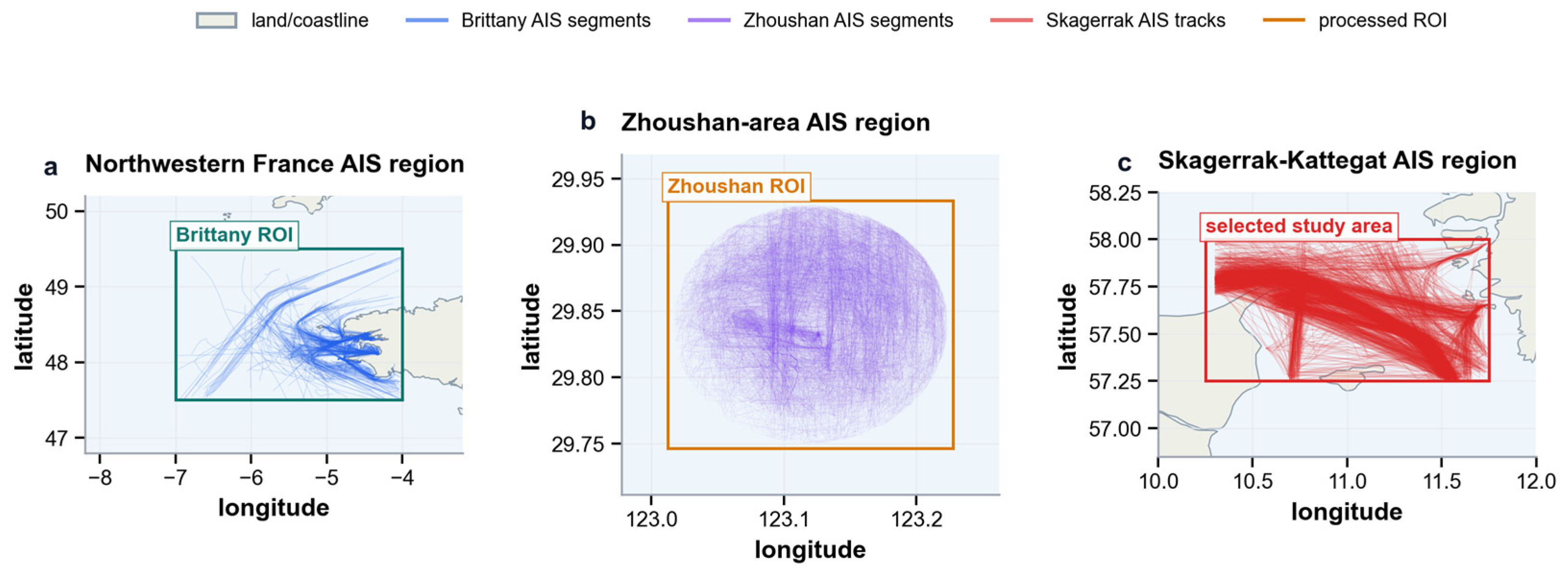
This study uses AIS records from three water areas. The Zhoushan dataset, collected approximately 100 km east of the Zhoushan Archipelago (centered at ${29.84}^{°} \mathrm{N},{123.12}^{°} \mathrm{E}$) in the East China Sea, is used for model training and validation. The Brittany dataset (northwestern France, ${47.5}^{°} \mathrm{N}$–${49.5}^{°} \mathrm{N}$, ${7.0}^{°} \mathrm{W}$–${4.0}^{°} \mathrm{W}$) and the Skagerrak dataset (Danish Maritime Authority (DMA) AIS records, ${57.25}^{°} \mathrm{N}$–${58.00}^{°} \mathrm{N}$, ${10.25}^{°} \mathrm{E}$–${11.75}^{°} \mathrm{E}$) serve as cross-water evaluation targets. The preprocessing pipeline described in Section 3.1 was applied identically to all three datasets. Figure 4 shows the vessel trajectory traces after ROI filtering;

Table 2. Processed AIS trajectory segments and experimental roles. Counts refer to trajectory-window samples after filtering, 5 min resampling, sliding-window construction, and trajectory-level downsampling of window samples.

Dataset	Region	Role	Samples	Period
Zhoushan	East China Sea	Training	53,959	Apr. 2020
Brittany	Northwestern France	Cross-water target	104,811	Nov.–Dec. 2016
Skagerrak	Skagerrak	Cross-water target	29,892	Jan.–Dec. 2019

summarizes the dataset statistics.

4.1.2. Baselines

We evaluate the proposed method against five architectures that span the main model families used in vessel trajectory prediction.

• LSTM [52]: the long short-term memory network captures temporal dependencies in sequential AIS data through gated memory cells, serving as the standard recurrent baseline for trajectory forecasting.
• GRU [11]: the gated recurrent unit offers comparable sequence modeling capability to LSTM with a simpler gating structure, providing a lighter recurrent alternative.
• BiLSTM [52]: a bidirectional LSTM that processes the trajectory in both forward and backward directions, testing whether access to future context within the observation window improves prediction.
• BiGRU [10]: a bidirectional GRU that combines the lightweight GRU cell with bidirectional processing, serving as a second bidirectional comparison point.
• Transformer [12]: the Transformer replaces recurrence with self-attention over the full observation window, and serves as the backbone of the proposed method, allowing the contribution of H3-indexed context to be isolated from backbone architecture effects.

All baselines are trained under the same hyperparameters and H3-aware objective (Section 3.4.1). The four recurrent baselines use one recurrent layer, hidden dimension 32, and dropout 0.2; the Transformer baseline uses the same architecture as the proposed backbone.

4.1.3. Training Configuration

Following the preprocessing pipeline described in Section 3.1, each trajectory segment is converted into a fixed-length input–target window. The input window consists of six observed time steps at a 5 min interval, and the prediction target is the 12-step (60 min) future displacement sequence. Each step provides four features: local east–north displacement and eastward–northward velocity components, normalized by fixed scale constants of $50,000$ m for position and 30 kn for velocity. Training, validation, and test sets are split chronologically before window extraction and H3 context construction to prevent information leakage. H3 context is constructed at resolution levels 7, 6, and 5, providing progressively coarser spatial context to capture traffic patterns at multiple scales. Resolution 7 (edge length $\sim$1.4 km) preserves local route-corridor structure and lane-level flow differences; Resolution 6 ($\sim$3.7 km) aggregates traffic over neighborhood-scale areas where multiple corridors converge; and Resolution 5 ($\sim$9.9 km) captures regional flow patterns spanning several route segments.

All models are trained with the AdamW optimizer [53] for at most 150 epochs with early stopping (patience of 40 epochs, minimum 50).

Table 3. Key training and architecture hyperparameters.

Component	Hyperparameter	Value
Architecture	Layers	2
	Hidden dimension	64
	Attention heads	4
	Feedforward dimension	128
	Dropout	0.1
Training	Optimizer	AdamW
	Learning rate	1 × 10−3
	Weight decay	1 × 10−4
	Gradient clipping	1.0
	Learning-rate schedule	Cosine + warmup
	Batch size	2048
H3-aware loss	Spatial tolerance	H3 res. 8, kring = 1

lists the key hyperparameters. The model is trained on the Zhoushan training set with checkpoint selection based on the Zhoushan validation set. For cross-water evaluation, each target-area dataset is similarly partitioned into training, validation, and test sets. Evaluation is then performed on the Zhoushan test set and on the test sets of the two cross-water datasets, each supplemented with H3 context maps constructed from the corresponding training portion.

The internal dimensions of each sub-module are as follows. The Transformer predictor receives the $L \times 4 =6 \times 4$ input sequence, projects it to $d_{\mathrm{m}\mathrm{o}\mathrm{d}\mathrm{e}\mathrm{l}}=64$ dimensions, and produces a $12 \times 2$ displacement forecast through a two-layer MLP horizon decoder (LayerNorm, Linear $384\to 256$, GELU, Dropout 0.1, Linear $256\to 24$, reshaped to $12 \times 2$). The candidate selector receives a 31-dimensional input per token and produces softmax weights over 15 candidates (LayerNorm, Linear $31\to 64$, GELU, Linear $64\to 1$; 2175 parameters). The final reliability gate receives a 20-dimensional input and produces ${\alpha }_{\mathrm{b}\mathrm{a}\mathrm{s}\mathrm{e}}\in [0,1]$ (LayerNorm, Linear $20\to 48$, GELU, Dropout 0.1, Linear $48\to 1$, Sigmoid; 1097 parameters). The full model contains 176,544 trainable parameters, of which the routing branch accounts for 3272 (1.85%).

All experiments were conducted on Ubuntu 22.04 with Python 3.12, PyTorch 2.8.0 and CUDA 12.8, using one NVIDIA GeForce RTX 5090 GPU (32 GB). Additional libraries include NumPy 2.3.2, pandas 3.0.3, Scikit-learn 1.9.0, h3 4.5.0, and Matplotlib 3.10.5.

4.2. Results

To assess the proposed method, the evaluation proceeds in three parts: baseline comparison on the training region identifies the strongest backbone architecture, cross-water-area evaluation measures geographic transfer against the same baselines, and a paired with/without comparison isolates the contribution of H3-indexed historical context.

Table 4. Baseline performance on Zhoushan.

Model	H3-ADE (km)	ADE (km)	FDE (km)	R2
Transformer	0.297	0.316	0.625	0.343
GRU	0.328	0.350	0.674	0.307
LSTM	0.337	0.361	0.686	0.282
BiGRU	0.320	0.323	0.628	0.357
BiLSTM	0.316	0.320	0.622	0.355

reports the baseline performance on the Zhoushan test set. The Transformer backbone achieves the best H3-ADE (0.297 km), ADE (0.316 km), FDE (0.625 km), and $R^2$ (0.343), followed by BiLSTM, BiGRU, GRU, and LSTM. With the Transformer backbone established as the strongest predictor on the training region, we now evaluate transfer performance across water areas.

To evaluate geographic transfer, all models trained on Zhoushan are tested on two additional water areas—Brittany and Skagerrak—without target-area fine-tuning.

Table 5. Cross-water-area H3-ADE (km). Brittany and Skagerrak are geographic-transfer targets. All models are trained on Zhoushan only. Target-domain values are mean $\pm$ SD over three independent training runs (seeds 42, 123, 456).

Model	Zhoushan	Brittany	Skagerrak
Transformer	0.297	1.807 ± 0.007	2.741 ± 0.015
GRU	0.328	1.729 ± 0.034	2.567 ± 0.099
LSTM	0.337	1.732 ± 0.019	2.551 ± 0.056
BiGRU	0.320	1.753 ± 0.020	2.622 ± 0.042
BiLSTM	0.316	1.799 ± 0.031	2.718 ± 0.078
Proposed	0.515	1.349 ± 0.034	1.413 ± 0.020

reports the H3-ADE of all five baselines and the proposed model on Zhoushan, Brittany, and Skagerrak; target-domain values are averaged over three independent training runs. On Brittany, the proposed model achieves the lowest H3-ADE (1.349 km), reducing the best baseline (GRU, 1.729 km) by 0.380 km. On Skagerrak, the proposed model reduces H3-ADE from the best baseline (LSTM, 2.551 km) to 1.413 km, a reduction of 1.138 km. 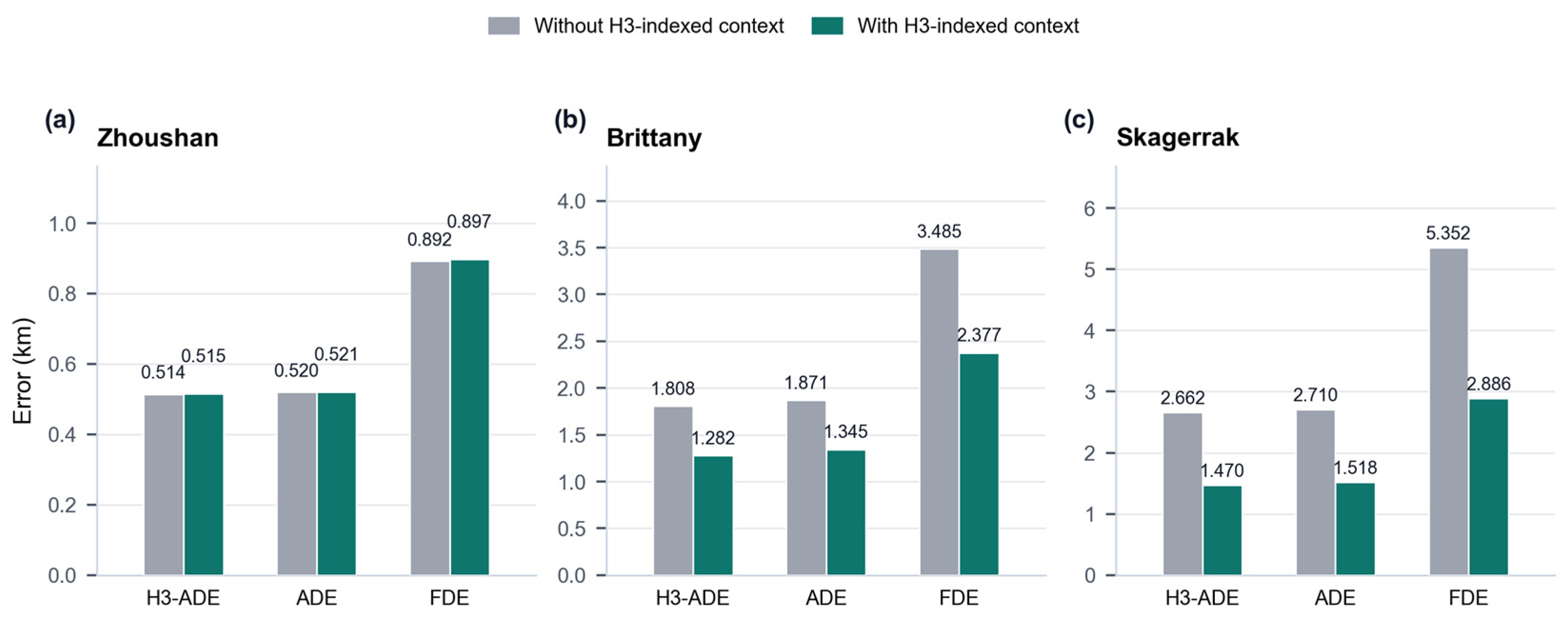Figure 5 further shows how the H3-indexed context changes the proposed model’s H3-ADE, ADE, and FDE across the three water areas.

Table 6. H3-indexed context contribution: H3-ADE (km) of the proposed model with and without H3 context. We define $\Delta ={\mathrm{H}3\text{-}\mathrm{A}\mathrm{D}\mathrm{E}}_{\mathrm{w}\mathrm{i}\mathrm{t}\mathrm{h}\mathrm{o}\mathrm{u}\mathrm{t}}-{\mathrm{H}3\text{-}\mathrm{A}\mathrm{D}\mathrm{E}}_{\mathrm{w}\mathrm{i}\mathrm{t}\mathrm{h}}$; thus, positive values indicate that H3 context reduces error. CIs are percentile 95% intervals from 10,000 paired bootstrap resamples. ${\widehat{\mathrm{P}\mathrm{r}}}_{\mathrm{b}\mathrm{o}\mathrm{o}\mathrm{t}}(\Delta >0)$ is the fraction of resamples with a positive reduction, not a hypothesis-test $p$-value.

Target	Without H3	With H3	Δ	95% CI	${\widehat{\mathit{P}\mathit{r}}}_{\mathit{b}\mathit{o}\mathit{o}\mathit{t}}$ (Δ > 0)
Zhoushan	0.5137	0.5150	−0.0013	[−0.0021, −0.0004]	0.0022
Brittany	1.8082	1.2819	0.5263	[0.5054, 0.5471]	1.0000
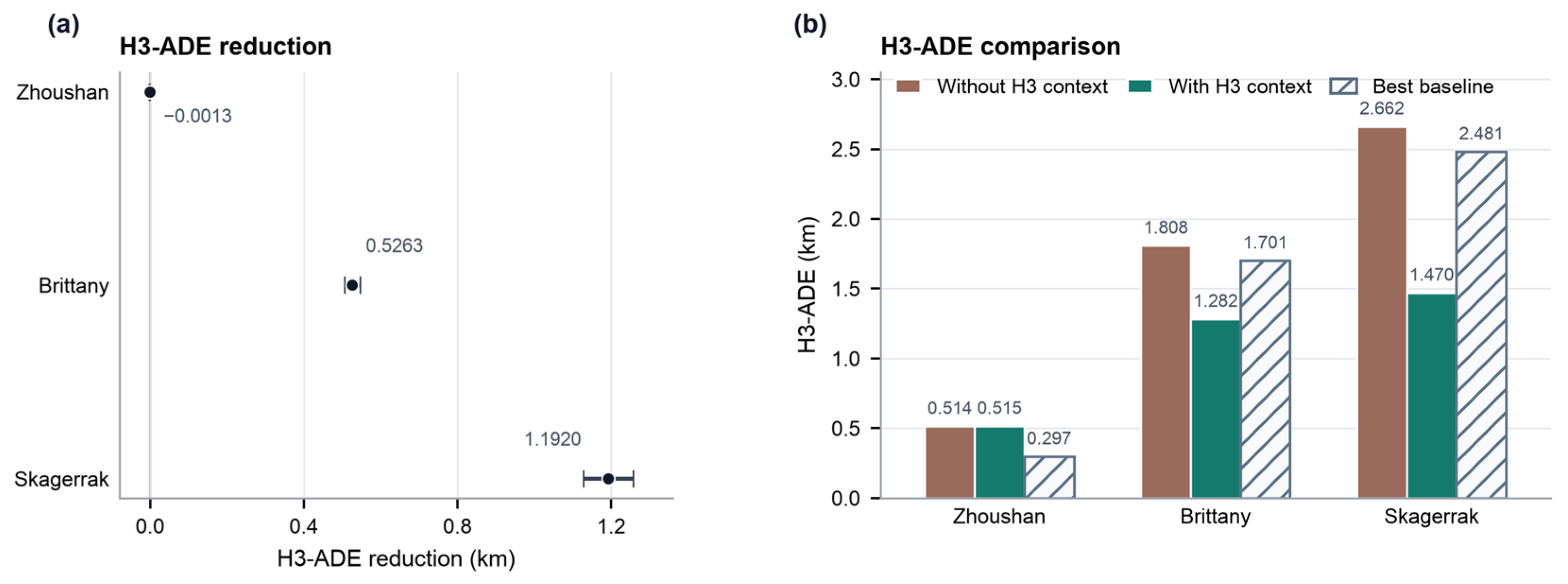
Skagerrak	2.6616	1.4696	1.1920	[1.1279, 1.2571]	1.0000

isolates the contribution of H3-indexed historical context by comparing the same trained model with and without H3 context on all three water areas. We define the paired H3-ADE reduction as $\Delta ={\mathrm{H}3\text{-}\mathrm{A}\mathrm{D}\mathrm{E}}_{\mathrm{w}\mathrm{i}\mathrm{t}\mathrm{h}\mathrm{o}\mathrm{u}\mathrm{t}}-{\mathrm{H}3\text{-}\mathrm{A}\mathrm{D}\mathrm{E}}_{\mathrm{w}\mathrm{i}\mathrm{t}\mathrm{h}}$, so positive values indicate lower error with H3 context. Paired-bootstrap 95% confidence intervals (CIs) were obtained from 10,000 resamples of the per-sample reductions. On Zhoushan, H3 context produces a practically negligible increase in H3-ADE of 0.0013 km: $\Delta =-0.0013$ km (95% CI $[-0.0021,\hspace{0.17em}-0.0004]$; ${\widehat{\mathrm{P}\mathrm{r}}}_{\mathrm{b}\mathrm{o}\mathrm{o}\mathrm{t}}\left(\Delta >0\right)=0.0022$). On Brittany and Skagerrak, H3 context reduces H3-ADE by 0.5263 km (95% CI $[0.5054,\hspace{0.17em}0.5471]$) and 1.1920 km (95% CI $[1.1279,\hspace{0.17em}1.2571]$), respectively; all 10,000 bootstrap resamples yield positive reductions for both targets.

4.3. Discussion

The results reveal a consistent pattern: H3-indexed historical context provides substantial improvement in cross-water transfer while having a practically negligible effect on the training region. This asymmetry clarifies the role of H3 context as a spatial prior rather than a generic feature enhancement. When training data are sufficient—as on Zhoushan, where the Transformer predictor already captures region-specific motion patterns—the selector suppresses most of the H3 contribution. The remaining $\Delta =-0.0013$ km corresponds to a 1.3 m increase in H3-ADE. Although its bootstrap interval excludes zero, this magnitude is too small to constitute a practically meaningful degradation. On geographically distinct targets, the H3-derived forecast supplies route-structure and speed-regime information that is absent from the training data, and the selector assigns it higher weight. The larger reduction on Skagerrak ($\Delta =1.1920$ km) than on Brittany ($\Delta =0.5263$ km) is consistent with Skagerrak being geographically more distinct from the training region. Figure 6 summarizes this pattern by pairing bootstrap uncertainty intervals with the H3-ADE comparison among the no-context model, the H3-context model, and the strongest baseline.

H3 context encodes aggregated statistics, but individual trajectory sequences may depart from these typical patterns. Rather than following the retrieved context unconditionally, the selector judges per sequence whether the vessel’s current motion and the retrieved context warrant relying on the H3-derived forecast, conditioning this decision on how strongly the retrieved context is supported and how concentrated its motion distribution is. When the two predictive sources diverge—for example, when the context carries low evidential weight or when the vessel’s motion does not align with the dominant traffic pattern—the selector can decline the H3 context and default to the motion-based forecast. This flexibility allows the model to draw on H3 context when it supplies informative traffic structure absent from the training data, without the H3-derived forecast overriding the motion-based forecast.

The practical significance of these findings lies in maritime situational awareness. H3-indexed context maps can be constructed entirely from historical AIS records without requiring target-area model training, making the proposed model applicable to water areas where labeled supervision data are scarce or unavailable. In operational settings such as Vessel Traffic Service centers, this enables rapid deployment of trajectory prediction in newly monitored regions using only archived AIS records as spatial context, without the cost and delay of collecting and annotating in-domain training data.

This compensatory mechanism is only as reliable as the AIS record from which the context is built. In well-observed coastal waters the context maps are densely supported and the selector draws on them confidently; in sparsely sampled regions the support score drops and the model falls back to its motion-based forecast—a graceful degradation that is by design, but which also means the H3 context adds no value in precisely the regions where external spatial priors might be most needed. The method’s reliance on AIS-derived position, speed, and heading further limits what the context can represent: environmental forcing, vessel-specific maneuverability, and sudden operational decisions all influence real-world motion yet leave no trace in the historical statistics. More fundamentally, the current implementation constructs context maps from a fixed historical window. Because context construction is decoupled from predictor training, however, the architecture naturally supports incremental refresh as new AIS data arrive; realizing this potential—tracking seasonal shifts, new routes, or regulatory changes without full recomputation—is a concrete direction for future work. The differing observation periods of the three datasets illustrate why such refresh mechanisms would be valuable, since long-term changes in vessel populations or routing patterns may gradually shift the patterns the backbone has learned.

The selector actively mitigates several of these issues. By attenuating the H3 contribution when the vessel’s kinematics diverge from the historical norm, it prevents stale or irrelevant context from overriding the motion-based forecast. This attenuation, however, operates on observed motion and cannot anticipate behavioral transitions that unfold within the prediction horizon: a vessel that abruptly shifts from transit to maneuvering will still receive flow statistics reflecting the dominant transit pattern, and even a small nonzero mixing weight can introduce a directional bias. Unanticipated behavioral transitions of this kind, together with the residual gap between cross-water prediction and target-area training accuracy, indicate that H3-indexed context is best understood as a complement to—rather than a substitute for—in-domain supervision and real-time situational awareness. The present evaluation covers three coastal environments with moderate-to-high AIS coverage; extending the approach to inland waterways, high-latitude routes, or regions with different traffic regulations would require broader validation, and scaling context construction to global coverage would benefit from GPU-accelerated spatial indexing.

5. Conclusions

This paper proposed a trajectory prediction method that incorporates H3-indexed historical traffic context into Transformer-based vessel trajectory prediction. H3 spatial indexing aggregates multi-resolution, speed-conditioned traffic statistics from historical AIS records, and a reliability-aware selector determines the contribution of these statistics to the final forecast.

The main findings of this study are as follows:

• H3 spatial indexing organized historical AIS records into structured, multi-resolution traffic context that can be integrated with a trajectory predictor as an additional information source.
• By combining this H3-indexed context with a Transformer-based predictor, the proposed model addressed the accuracy degradation that typically accompanies cross-water transfer while maintaining strong performance on the training region.
• The combination of H3-indexed context and Transformer-based prediction offers a promising architecture for trajectory prediction tasks that benefit from external spatial knowledge, and provides a foundation for incorporating richer contextual information.

These findings should be interpreted in light of the method’s practical costs and evaluation scope. Constructing the H3 context maps required 5–27 s per region and 389 MiB of serialized storage for the three regions evaluated; the routing components added 3272 parameters (1.85% of the full model) and approximately 1.8 ms of inference overhead per batch. While these costs are modest at the scale of the present study, they would grow proportionally for global-scale deployment and would require periodic recomputation to reflect evolving traffic patterns. The evaluation was conducted on three coastal or near-shore maritime environments with moderate-to-high AIS coverage; performance in inland waterways, high-latitude routes, sparsely sampled regions, or areas with markedly different traffic regulations has not been assessed.

Future work will extend the H3-indexed context framework along several directions. Richer operational, environmental, and intent-related context could be incorporated to improve prediction under low-speed, adverse, or weakly represented traffic conditions; in particular, reformulating the context as structured knowledge that could be combined with large language models, expert knowledge, and domain knowledge would enable more flexible, description-level reasoning about exceptional conditions. Incremental context-update mechanisms that track evolving traffic patterns without full recomputation would improve long-term operational relevance. The current H3 indexing and retrieval implementation relies on CPU-based library calls; GPU-accelerated spatial indexing and context retrieval could reduce latency in high-throughput operational settings. Broader evaluations across additional geographic regions and maritime scenarios would further clarify the method’s performance boundaries. These directions suggest that H3-indexed historical traffic context can serve as a practical spatial interface for enriching AIS trajectory prediction with structured, reusable traffic knowledge.