Method for Calculating a Generic Oil

Abstract

Accidental oil spills are an all-too-common occurrence. In order to properly plan for and respond to oil spills, responders and planners need to understand how the oil will behave in the environment: how it will weather and how it will affect ecosystems and biota. To address this need, databases of oil properties have been developed, such as NOAA’s Automated Data Inquiry for Oil Spills (ADIOS^®) Oil Database, a publicly available database of oil properties useful for oil spill modelers, responders, and planners, currently containing over 1400 oil records. However, despite its size, when a spill occurs, the actual oil spilled is unlikely to be in the database, even if the oil’s identity is known. The challenge is even greater for planners, who cannot possibly plan for the spilling of thousands of individual different oils. When the exact product is not available, the responder must choose an oil record from the database that closely resembles the product at hand. This process can slow the responder down and may require them to have years of experience to choose the most appropriate oil record. If not done with care, a user can inadvertently select an atypical oil with a similar name, or a record with poor data quality, which can yield inappropriate results. In this work, we generated a set of “generic” oil records for the ADIOS^® Oil Database that have been developed to be a good representation of typical products of a certain type, e.g., “medium crude” or “diesel fuel”. These oil records can then be used in the early stages of a response when details about the spilled product are sparse. These generic oil records can also be very helpful for drills, training, and planning when the user does not need to work with a specific product. These generic records were developed by examining the extensive dataset available in the ADIOS Oil Database and determining which records matched a given type of oil and were of sufficient quality. Then all the records for each oil type were combined to create a “typical” or “average” oil that is representative of that oil type. In the course of this project, statistical methods were chosen that were most appropriate to the property at hand. The oil types chosen were: Light, Medium, and Heavy Crude, Condensate, Jet Fuel, Diesel, Gasoline, Intermediate Fuel Oil (IFO), and Heavy Fuel Oil (HFO). These are all oil types that are likely to be spilled, and for which sufficient data existed in the ADIOS Oil Database to compute an “average” oil. Other potential product types could be added in the future should more data become available.

1. Introduction

The Automated Data Inquiry for Oil Spills (ADIOS^®) Oil Database [1,2] contains approximately 1400 oil records which have been maintained and curated for over 30 years by the National Oceanic and Atmospheric Administration’s (NOAA) Emergency Response Division (ERD) to inform oil spill responders, particularly for predicting the fate and effects of spilled oil. However, its utility can be limited for a spill event, since the exact product involved in an actual oil spill is typically unknown. Even when the identity of the spilled product is known, it is rare for a good quality record of that exact product to be available. When the exact product is not available in the ADIOS Oil Database, the responder must use their best judgment to choose an oil record that closely resembles the product at hand. This process can slow the responder down and may require them to have years of experience to choose the most appropriate oil record. If not done with care, a user can inadvertently select an atypical oil with a similar name or a record with poor data quality, which can yield inappropriate results.

One solution to this problem is to have a set of “generic” oil records that have been developed to be a good representation of typical products of a certain type, e.g., “medium crude” or “diesel fuel”. These oil records can then be used in the early stages of a response when details about the spilled product are sparse. These generic oil records are also very helpful for drills, training, and planning when the user does not need to work with a specific product.

A set of generic oil records, with average and representative physical properties, was developed for the purpose of tackling this problem. Generic records were developed for nine oil types which are commonly transported and could be spilled, and for which there were sufficient data in the database. The oil types chosen were Light, Medium, and Heavy Crude; Condensate; Jet Fuel; Diesel; Gasoline; Intermediate Fuel Oil (IFO); and Heavy Fuel Oil (HFO). Other potential product types could be added in the future should sufficient data become available.

1.1. Contents of a Generic Record

The generic records were developed to define properties of a product that are most useful in the initial stages of an oil spill response [3]—for understanding health and safety issues, predicting oil behavior early in a spill, and properties which are critical inputs for oil spill weathering and trajectory models [4].

1.1.1. Properties Chosen

Pour Point: Used to understand how an oil might behave at colder temperatures; specifically, at what temperature it may behave as a gel or semi-solid rather than a liquid.

Flash Point: Critical for responder health and safety, as it indicates the lowest temperature at which oil vapors can be ignited.

Density: To understand if an oil product will sink or float in water. Density varies with temperature and as the oil weathers—models need a good estimate of the oil’s initial density as a function of temperature in order to model this property [5].

Viscosity: Affects potential response techniques and interaction of oil with the shoreline, and is used in weathering and trajectory models to calculate rate of spreading and tendency to emulsify.

Density and viscosity change with temperature, so values were determined at three temperatures (0, 15, and 25 °C) to cover a range of common environmental conditions.

SARA fractions (Saturates, Aromatics, Resins, and Asphaltenes): This compositional analysis is sometimes used in weathering models to calculate rates of weathering processes that depend on the chemical composition of the oil, such as biodegradation and emulsification [6,7].

Emulsification Behavior: Some oils will emulsify under certain conditions, typically after having weathered to some degree. For each oil, two values were determined: the fraction of the oil needed to evaporate before an emulsion would form (also called the “emulsification constant”), and the maximum water content of the resulting emulsion. For oils that will never emulsify, the emulsification constant is set at 100% (i.e., 100% of the oil must evaporate before formation of an emulsion; thus, an emulsion will never be formed) [8]. The emulsification behavior was determined from records for which laboratory analysis of emulsion formation was available.

Distillation Curve: Critical for understanding evaporation and persistence of oil in the environment. A distillation curve is a breakdown of a whole oil into mass fractions according to their boiling point. Distillation data are used in GNOME and other oil weathering models to predict evaporation and generate pseudo-components that are then used to track the progress of weathering over time [5,9].

1.1.2. Oil Types Selected

We chose to create generic records for the following types of oil: Light Crude, Medium Crude, Heavy Crude, Condensate, Jet Fuel, Diesel, Gasoline, Intermediate Fuel Oil (IFO), and Heavy Fuel Oil (HFO). These were chosen because they are the most commonly stored and transported petroleum products in the United States and because of that they are also the most frequently spilled [10]. There were also sufficient data in the ADIOS Oil Database to create useful generic records for these oil types. There are other, slightly less common oil types that we would have liked to have included, such as Dilbit (Diluted Bitumen) and Tight Oil (shale oils, fracking oil), for which there were not enough data available in the ADIOS Oil Database to create a quality generic record.

1.1.3. A Note on Low Sulfur Fuel Oils (LSFOs)

The diesel, IFO, and HFO generic records include data from all the records in the database, going back many years, even though since 2020 these fuels have been mandated to have a low sulfur content (0.5% or lower). The data from the old and new records were averaged together for a couple of reasons.

For diesels, an analysis was done of the diesels in the ADIOS Oil Database from before 2020 compared with diesel fuels produced after 2020 (

Table 1. Comparison of properties of pre- and post-2020 diesels.

Oil Type	API Gravity	Asphaltene Content, wt%	Flash Point, (°C)	Pour Point (°C)	Sulfur Content (wt%)	Viscosity at 37.8 °C (cSt)
Low Sulfur Diesels in ADIOS DB, 3 samples from 2020 to 2021	35–37	0.01	61.1–71.1	−39 to −13.3	0.01–0.05	2.35–3.8
Marine Diesel in ADIOS DB, 14 samples from 1994 to 2018	28.2–41.2	0–0.03	53.9–97.8	−36.5 to −4	0–0.1	3.7–7

). The properties of the post-2020 diesel generally fell within the range of the properties of the pre-2020 diesels, so we determined that the newer diesels were likely to behave similarly to older ones when released into the environment. Therefore, separate generic records for pre- and post-2020 diesels were not needed, and it was better to use the larger combined dataset to capture the variability between fuels.

For residual fuels, a similar analysis (

Table 2. Comparison of properties of pre- and post-2020 residual fuels with API Gravity > 15.

Oil Type	API Gravity	Asphaltene Content, wt%	Flash Point (°C)	Pour Point (°C)	Sulfur Content (wt%)	Viscosity at 15 °C (cP)
Post-2020 Residual Fuels with API > 15 in ADIOS DB, 29 samples from 2020 to 2024	15–27.9	0.3–10.6	65–176	−36 to 33	0.08–0.5	348–327,173
Pre-2020 Residual Fuels with API > 15 in ADIOS DB, 7 samples from 1999 to 2016	16.3–30.6	5.2–6	53.9–91.1	−24 to 24	0.6–1	59–4300

and

Table 3. Comparison of properties of pre- and post-2020 residual fuels with API Gravity < 15.

Oil Type	API Gravity	Asphaltene Content, wt%	Flash Point (°C)	Pour Point (°C)	Sulfur Content (wt%)	Viscosity at 15 °C (cP)
Post-2020 Residual Fuels with API < 15 in ADIOS DB, 15 samples from 2019 to 2022	10.3–14.3	0.73–17.83	70–137.8	−27 to 33	0.45–2.47	892–29,377
Pre-2020 Residual Fuels with API < 15 in ADIOS DB, 22 samples from 1992 to 2015	10.2–14.9	5–19	60–174	−24 to 38	0.5–2.7	1410–48,000

) showed that in some ways, post-2020 residual fuels were similar to pre-2020 fuels of similar API gravity, but that there was a wider variation in the values of some of the properties for the newer fuels.

Furthermore, the experiences of the global spill response community with these heavier LSFOs in the past few years have shown that there is not really such a thing as an average or typical heavy LSFO [11]. In particular, there is a wide variability in the pour point and viscosity of residual LSFOs. This is due to the differing sulfur contents of feedstock crude oils, and the fact that more intense hydrodesulfurization needs to be done to higher-sulfur feedstocks than to lower-sulfur feedstocks. This extra hydrodesulfurization process results in the transformation of aromatics and asphaltenes to waxes in some batches of LSFO and not others, affecting pour point and viscosity in particular [12]. Because of this, we decided that a generic record averaging the values of residual LSFOs would not be a good representation of any given residual LSFO, and could be misleading.

That being said, there is a record in the ADIOS Oil Database (AD02580) with data from a study carried out by the Australian Maritime Safety Authority [12], which has average properties from 48 samples of RMG 380 (Residual Marine Grade G 380), a specific type of residual LSFO, collected from commercial vessels visiting Australian ports in 2020–2021. While this record is not officially a generic oil record generated by the process described below, it can act as a generic RMG 380 record for modeling purposes.

2. Methods

2.1. Oil Categorization

In the petroleum industry, there is a huge variety of products, with a number of different and often overlapping ways to name and categorize any given product. This is particularly true of fuels and other refined products. This makes it challenging to know exactly what may have been spilled when initially reported.

For the purposes of this project, we sought to categorize oils with similar physical properties and behavior in the environment, aligned with how a product might be described in the event of a spill.

In the ADIOS Oil Database, the Product Type is a broad identifier of the general class of product. Essentially, the product type defines what the product “is”, and as such, each oil record is assigned only one Product Type. Within a given product type, for example, Crude Oil NOS (Not Otherwise Specified), there can be subcategories, such as “Medium Crude”. The generic oil categories are, in general, subcategories of broader product types.

Many of the records were not specifically defined by the original data source as to exactly which category they belong, such as what type of distillate fuel is described by a record. For oil records which were not previously categorized before this project, criteria were developed to assign categories based on physical properties of the oils. The categorization was then screened by staff to ensure accuracy and consistency.

The following criteria were used to screen and assign oil records to the various categories used for generic oil records:

• American Petroleum Institute (API) gravity
• Kinematic viscosity at a particular temperature (usually 50 °C).

The values used for each criterion for the different oil types can be found in

Table 4. Criteria used to categorize the oil data records in the ADIOS Oil Database.

Oil Type	API Gravity Min.	API Gravity Max.	Kin. Visc. (cSt) Min.	Kin. Visc. (cSt) Max.	Kin. Visc. Temperature (°C)
Light Crude	35	50	−∞	∞	15
Medium Crude	20	35	−∞	∞	15
Heavy Crude	−∞	20	−∞	∞	15
Condensate	50	∞	−∞	∞	15
IFO	11.5	30	4	380	50
HFO	−∞	12.5	−∞	∞	50
Gasoline	54.5	76.6	−∞	2.5	38
Jet Fuel	43	54.4	−∞	∞	38
Diesel	30	39	2	4	38

∞—infinity.

, and were found in various industry references, including Raymond & Leffler [13] for crude oil API ranges, and information from the US Energy Information Administration website [14] for the other products. Note that for intermediate and heavy fuel oils, the properties of the specifications overlap, so that categorization is not clearly defined when working only from the data. In the overlap between those two categories, records were manually reviewed after the automatic categorization step, and adjustments were made based on other information in the records, such as the name of the oil.

Categorization was performed for the following oil categories:

• Light Crude;
• Medium Crude;
• Heavy Crude;
• Condensate;
• Intermediate Fuel Oil (IFO;)
• Heavy Fuel Oil (HFO);
• Gasoline;
• Jet Fuel (grouped with kerosene);
• Diesel Fuel.

2.2. Statistical Methods

The data used to generate the generic oil records were taken from the complete set of records in the ADIOS Oil Database [2] as of December 2025.

For each generic oil record, all of the records in the database within the relevant category were selected. All the selected records were then screened for data errors and inconsistencies. This process identified a number of issues with the data. Each problematic record was either corrected or removed from the selection if the original correct data could not be found.

2.2.1. Temperature-Dependent Properties

Density and viscosity vary with the temperature of the product. Each generic oil record has average density and kinematic viscosity values computed for 0, 15, and 25 °C, to cover the range of likely temperatures in the environment.

Measured data at these temperatures were used when available. For records with measurements at other temperatures or with fewer measurements, density and viscosity values at the target temperatures were interpolated according to the method used in the General NOAA Operational Model (GNOME) oil weathering model [15].

Density

Average density at each temperature was computed as the arithmetic mean (Equation (1)) of all the records:

$$\mathrm{A}={\displaystyle \frac{1}{\mathrm{n}}}{\sum }_{\mathrm{i}=1}^{\mathrm{n}}{\mathrm{a}}_{\mathrm{i}}$$

(1)

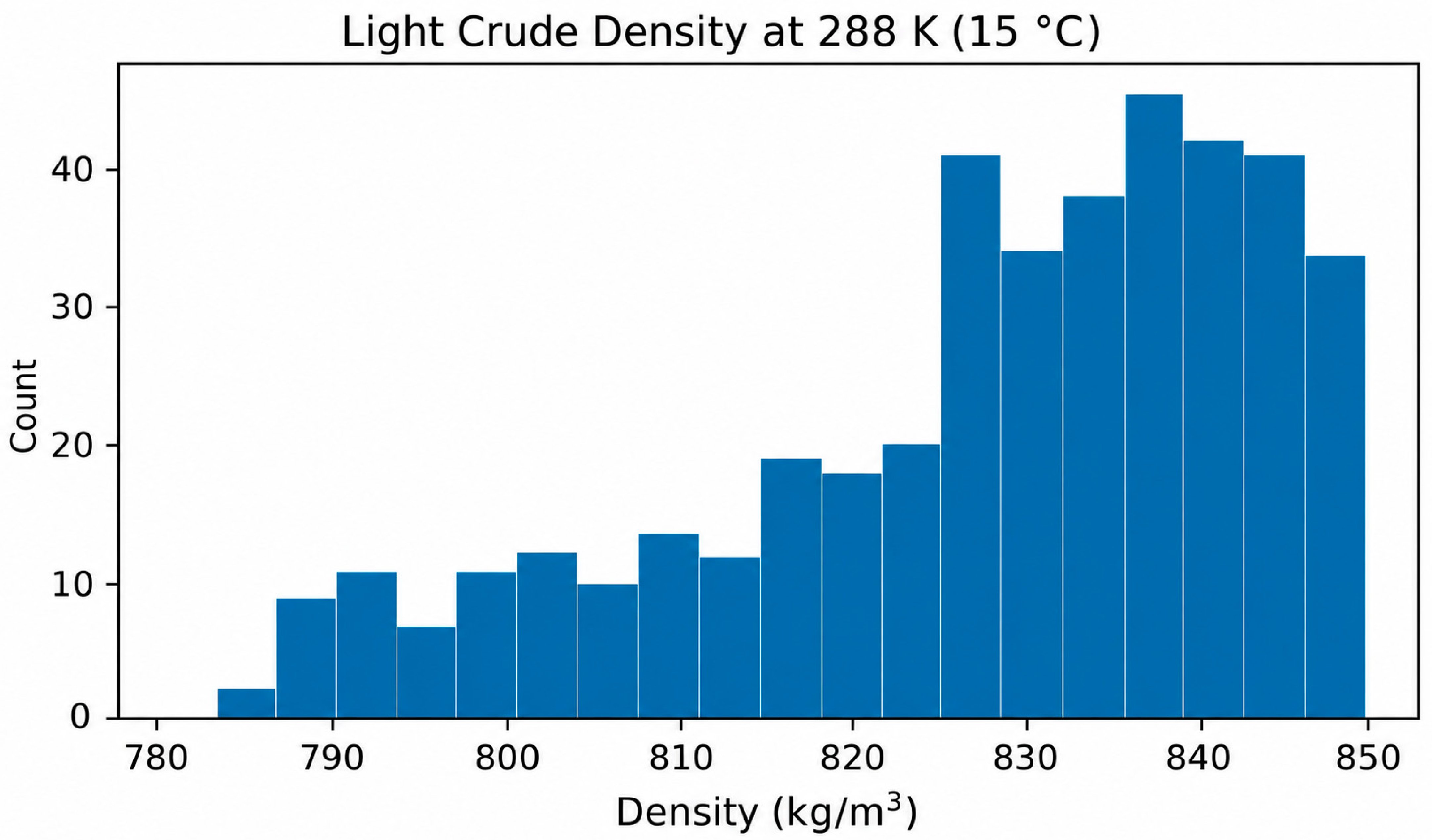
where A is the arithmetic mean, n is the number of records, and a_i are the individual data set values of the property. The data are fairly normally distributed, so the arithmetic mean is appropriate for these data. An example of a typical density distribution is given for Light Crude oils in Figure 1.

Kinematic Viscosity

Kinematic viscosity is known to vary widely, both with different materials and with temperature. To accommodate this, viscosity is often displayed on a log-scaled graph. This wide variation is reflected in the data: there is a very wide range of values, and the data are not normally distributed, with a very high skewness. Directly using an arithmetic mean for these data is not appropriate. To account for this and generate appropriate statistics, the skewness of all of the properties, including kinematic viscosity, was evaluated, and the results can be found in

Table 5. Skewness of Properties among Oil Types.

Oil Type	T (°C)	Dens. Skew	Visc. Skew	Pour Point Skew	Flash Point Skew	SARA Skew	Max. Water Content Before Emuls. Skew	Frac. Evap. Before Emuls. Skew
Light Crude	0	−0.664	5.499			Sat: 0.549
	15	0.0384	3.667	−0.110	0.913	Aro: −0.160	−1.103	−0.333
	25	1.541	4.017			Res: 0.027
						Asp: 1.629
Medium Crude	0	0.679	7.986			Sat: 0.077
	15	0.726	9.925	0.063	0.970	Aro: −0.092	−1.263	0.882
	25	0.702	9.491			Res: 1.576
						Asp: 1.231
Heavy Crude	0	0.110	6.520			Sat: 0.157
	15	0.196	3.724	0.470	2.095	Aro: −0.026	−1.685	1.693
	25	0.191	2.785			Res: −0.307
						Asp: 0.056
Condensate	0	−0.459	2.135			Sat: 0.090
	15	−0.459	1.511	1.012	0.321	Aro: 0.073	N/A	N/A
	25	−0.459	1.685			Res: N/A
						Asp: 0.140
IFO	0	−0.617	1.385			Sat: 0.568
	15	−0.205	1.802	0.743	−1.010	Aro: −0.711	−3.75 × 10−6	N/A
	25	0.301	1.885			Res: 0.975
						Asp: 0.417
HFO	0	0.759	0			Sat: N/A
	15	0.759	0	−0.453	−0.440	Aro: N/A	N/A	N/A
	25	0.759	0			Res: N/A
						Asp: 0.559
Jet Fuel	0	1.071	0.324			Sat: N/A
	15	1.212	0.415	−0.229	0.759	Aro: −0.756	N/A	N/A
	25	−0.215	0.451			Res: N/A
						Asp: N/A
Diesel	0	0.782	1.995			Sat: −0.468
	15	0.796	0.937	−0.376	0.213	Aro: 0.489	N/A	N/A
	25	0.756	0.576			Res: −1.500
						Asp: 0.845
Gasoline	0	−0.213	−0.361			Sat: N/A
	15	−0.391	−0.343	0.671	0.558	Aro: 0.426	N/A	N/A
	25	−0.532	−0.355			Res: N/A
						Asp: N/A

. Skewness for kinematic viscosity ranges from the various properties range from 1.685 to 9.925, with most well above 2.0—generally considered a threshold for “Severely Non-Normal”. The skewness for the rest of the properties is mostly well below 2.0, and the arithmetic mean is a reasonable estimate for the central mean value—transformation of these data would not significantly affect the results.

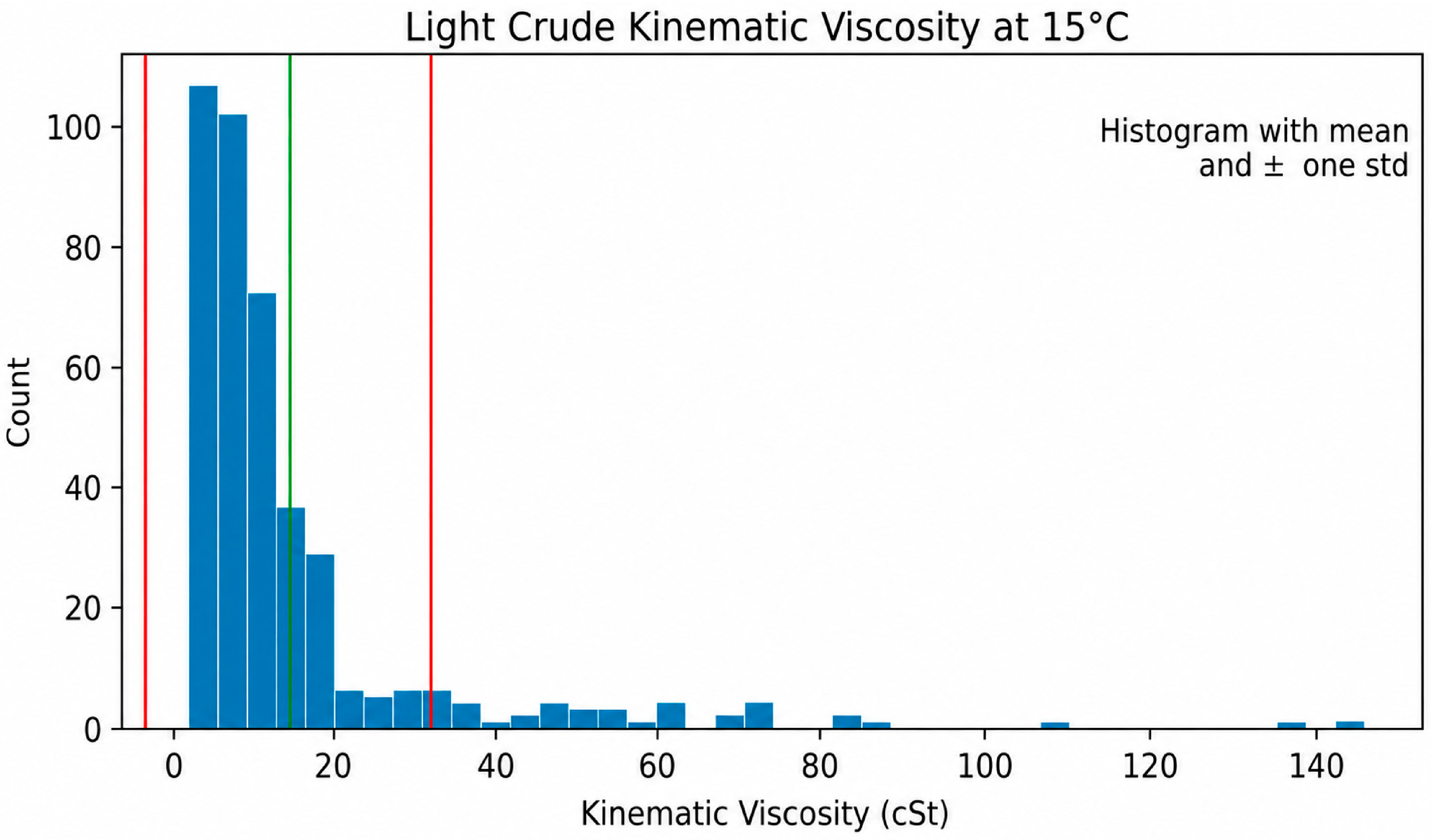
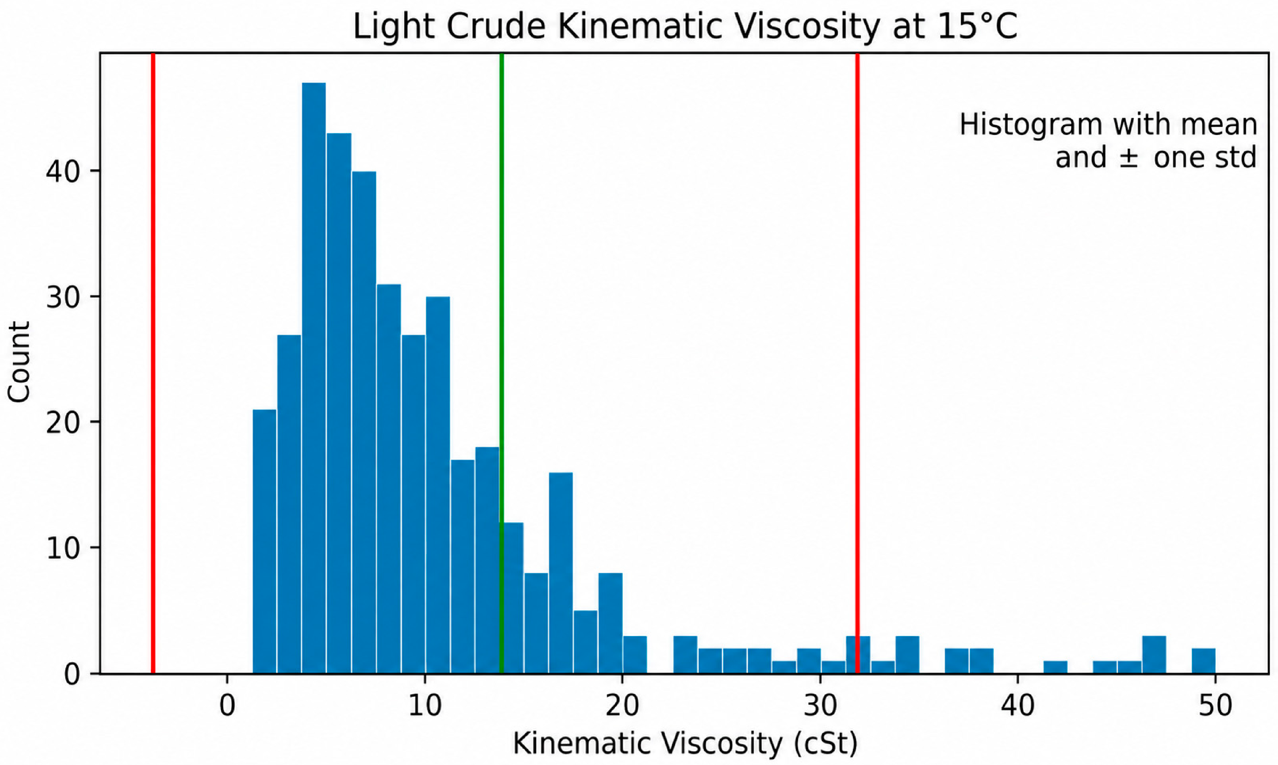
Examination of histograms of the kinematic viscosity data for all the oil types corroborates the skewedness of this dataset. For example, a histogram for the kinematic viscosity data for Light Crudes at 288 K (15 °C) is shown in Figure 2. From this, it can be clearly seen that the data are highly skewed (skewness of 3.67), with most of the values within a fairly small range (70% of the values in the first three bins, between 1.75 cSt and 12 cSt), and a small number of values far outside this range. If the mean and standard deviation are derived from the raw data, unreasonable values will result, with a mean of ~14 cSt and a standard deviation of ~18 cSt.

Figure 3 shows the same histogram, focusing on where most of the data are. This clearly shows that the mean is not near the central value for the data, and that the range within one standard deviation of the mean falls well outside the limits of the data, causing the inclusion of physically meaningless negative values. For this reason, a further transformation was applied to the kinematic viscosity data before the averages were calculated.

A common statistical technique for deriving statistics from skewed data is to transform the data into a normally distributed range, compute the statistics on the transformed data, and then transform back for meaningful results. For this project, the Box–Cox transformation [16] was used to normalize the kinematic viscosity data to more closely approximate a normal distribution.

The Box–Cox transformation of the variable y is indexed by λ, and is defined as:

$$\mathrm{y}\left(\mathrm{\lambda }\right)={\displaystyle \frac{{\mathrm{y}}^{\mathrm{\lambda }}-1}{\mathrm{\lambda }}},\hspace{1em}\hspace{1em}\mathrm{i}\mathrm{f} \mathrm{\lambda }\ne 0$$

(2)

$$\mathrm{y}\left(\mathrm{\lambda }\right)=\mathrm{l}\mathrm{o}\mathrm{g}\left(\mathrm{y}\right),\hspace{1em}\hspace{1em}\mathrm{i}\mathrm{f} \mathrm{\lambda }=0$$

(3)

The exponent, λ, can vary between −5 and 5. An optimal value is chosen that shifts the dataset to the best approximation of a normal distribution.

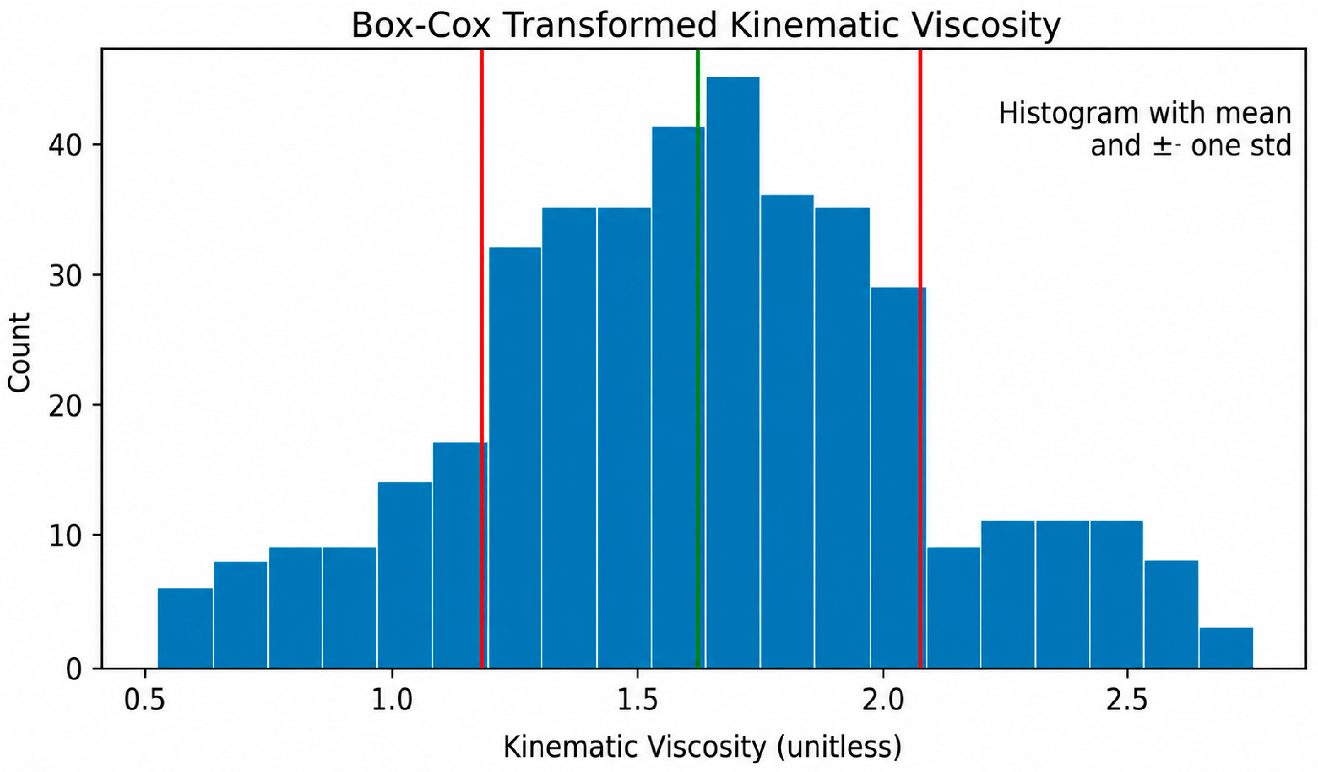
Figure 4 shows the histogram of the kinematic viscosity data after transforming with a Box–Cox transform (λ ≅ 0.265). The transformed data are fairly normally distributed, with skewness of 0.015, mean of 1.62 and standard deviation of 0.45. In this case, the mean is near the center of the data, and the bulk of the data falls within one standard deviation of the mean.

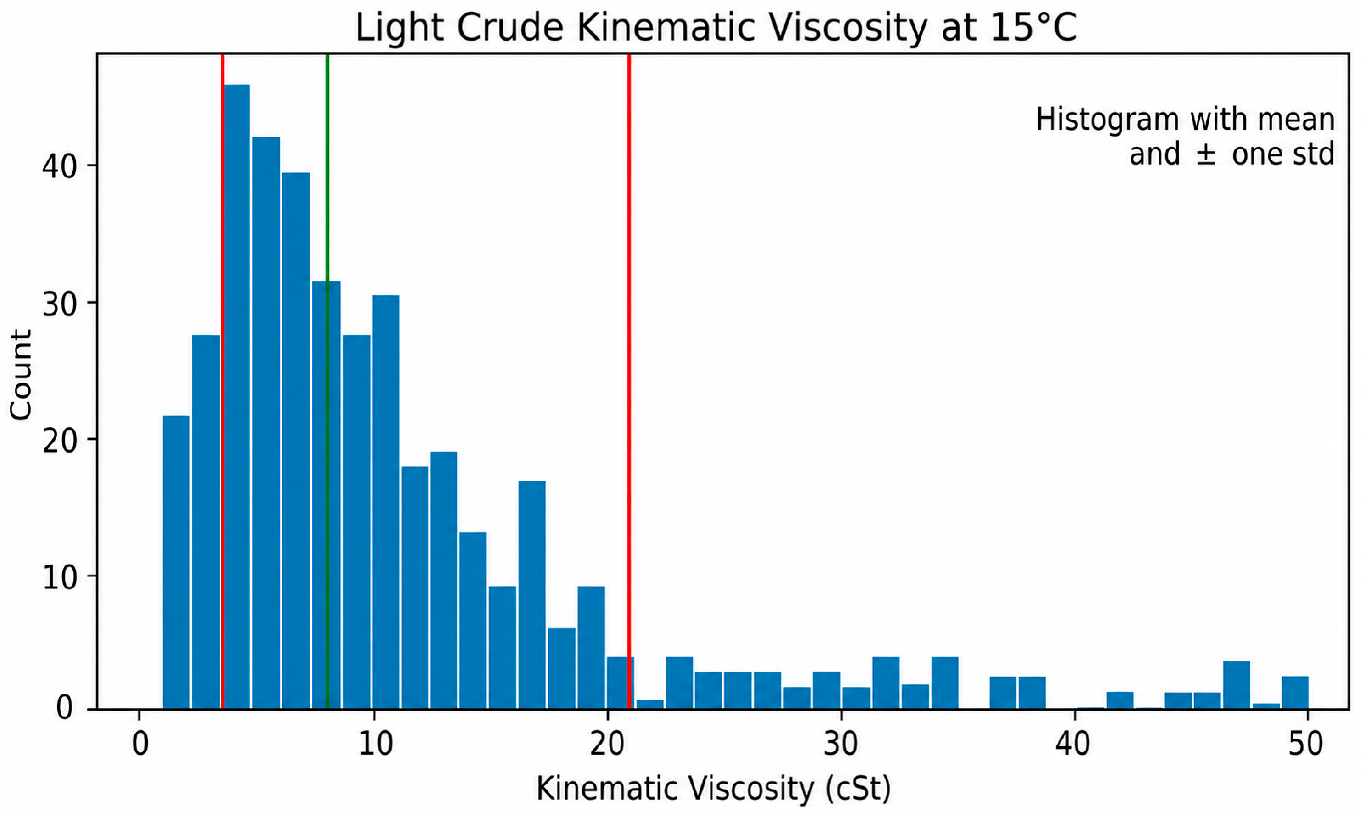
Figure 5 shows the original viscosity data, the same as Figure 4, but with the mean and bounds after reverse transformation back to units of cSt. It is apparent that the mean value lies near the center of the data, and most of the data is within one standard deviation of the mean, indicating that the transform produced a good representation of the “average” viscosity of these data. The same procedure was applied to the kinematic viscosity data of all of the oil types processed.

2.2.2. Temperature-Independent Properties

Four additional temperature-independent properties were evaluated for each category of oil. These properties are: pour point, flash point, and two experimentally determined emulsion parameters: the fraction of oil evaporated before formation of an emulsion (emulsification constant), and maximum water content incorporated into the resulting emulsion. The data for all of these properties generally fell into a normal distribution (e.g., had moderate skewness), so a standard arithmetic mean (Equation (1)) was used for each of these properties. Additionally, for the oil types that had SARA data available, the arithmetic mean of the SARA concentrations was determined.

2.2.3. Distillation Curve

A similar process was used to calculate distillation curves. The first step was a quality check in which records/samples with problems (missing distillation fractions, out-of-order fractions, not having enough distillation cuts or the initial/final fraction being too high or low, which indicates missing data) were removed from the analysis.

For each valid record, a distillation curve was calculated by interpolating from the existing data, and a new table of distillation temperatures, from 0 to 100% mass fraction in increments of 5%, was generated based on the calculated curve. This ensured that all of the records had distillation cuts reported at the same standardized mass fraction values. For each product category, an average curve was computed by averaging the boiling point temperatures of all records for each fraction. For example, the boiling point temperatures at 5% distilled of all the gasoline records were averaged together using a simple arithmetic mean to give the boiling point temperature at 5% distilled for the generic gasoline record.

2.2.4. Outliers

In the initial analysis, there were a number of outliers in the data, particularly the kinematic viscosity data. For kinematic viscosity, these were identified by how far they deviated from the standard deviation after the Box–Cox transformation. Each outlier was examined to determine why it contained an extreme value, and most of the outliers turned out to be a result of errors in the original data or in the method originally used to extrapolate the viscosity from measured data. These errors were corrected within the database, when possible.

Remaining outliers that were not data errors were also removed from the analysis, under the assumption that they were not representative of a typical product. These outliers were identified by applying an Interquartile Range (IQR) analysis, which measures the statistical dispersion of each dataset. This is done by computing the difference between the first (Q1) and third quartiles (Q3) (25 and 75%):

$$\mathrm{I}\mathrm{Q}\mathrm{R}=\mathrm{Q}3-\mathrm{Q}1$$

(4)

$$\mathrm{L}\mathrm{o}\mathrm{w}\mathrm{e}\mathrm{r} \mathrm{B}\mathrm{o}\mathrm{u}\mathrm{n}\mathrm{d}=\mathrm{Q}1-1.5 \ast \mathrm{I}\mathrm{Q}\mathrm{R}$$

(5)

$$\mathrm{U}\mathrm{p}\mathrm{p}\mathrm{e}\mathrm{r} \mathrm{B}\mathrm{o}\mathrm{u}\mathrm{n}\mathrm{d}=\mathrm{Q}3+1.5 \ast \mathrm{I}\mathrm{Q}\mathrm{R}$$

(6)

If a datapoint in question was less than the Lower Bound or higher than the Upper Bound, it was considered an outlier and removed from the dataset. The IQR analysis was performed on the transformed data, where appropriate.

2.2.5. Summary

A summary of the number of records removed as a result of the statistical analysis is shown in

Table 6. Number of records in each category before and after statistical analysis.

Oil Type	Number of Records After Initial Categorization Based on API Gravity and Kinematic Viscosity	Number of Records Left After IQR Analysis and Removal of Outliers
Light Crude	442	421
Medium Crude	524	476
Heavy Crude	90	82
Condensate	35	26
IFO	14	11
HFO	8	7
Gasoline	19	19
Jet Fuel	16	12
Diesel	31	28

. Note that the number of and quality of records available for a given category varied widely. As a result, some generic records with less data may not represent an “average” oil of that category as well as generic records with more underlying data. However, we have only included oil types for which there was enough data to provide a useful record—the generic record will still capture a central tendency and better represent the oil’s behavior than selecting an arbitrary record.

For some properties, such as SARA analysis and emulsification data, even less data were available. However, the properties with less data happen to be less important to oil spill modeling, so while there is greater uncertainty in these values, the precision of the results is less critical to responders. Additional data are constantly being added to the ADIOS Oil Database, and these generic records will be updated in the future when more data become available.

3. Results

Generic oil records were generated for nine specific oil categories, including light, medium, and heavy crude, condensate, jet fuel, heavy fuel oil, intermediate fuel oil, diesel, and gasoline. Results for each property are shown in this section, and the complete generic oil records are included in the Supplementary Materials.

3.1. Density and Kinematic Viscosity

Average density and viscosity values and the statistics of these analyses are presented in

Table 7. Average density and kinematic viscosity for nine generic oils.

Oil Type	Product Type	Records Used in Analysis	T (°C)	Average Density (kg/m3)	Average Kinematic Viscosity (cSt)	Avg. K. Visc + Std Dev. (cSt)	Avg. K. Visc − Std Dev. (cSt)	Box-Cox λ
Light Crude	Crude Oil NOS	421	0	829.3 ± 17.1	18.9	59.6	7.2	−0.172
			15	828.0 ± 17.1	8.3	20.4	4.1	−0.266
			25	827.3 ± 18.2	5.3	12.3	2.5	−0.150
Medium Crude	Crude Oil NOS	476	0	881.9 ± 23.4	114.3	696.8	30.5	−0.202
			15	879.1 ± 22.6	40.4	173.9	14.5	−0.286
			25	877.4 ± 23.0	22.6	90.7	7.9	−0.228
Heavy Crude	Crude Oil NOS	82	0	968.4 ± 22.2	29,571	312,891	2514	0.018
			15	963.6 ± 20.9	6228	48,839	705	0.026
			25	960.4 ± 21.4	2374	15,974	318	0.026
Condensate	Condensate	26	0	751.9 ± 16.0	2.96	12.6	1.05	−0.278
			15	751.9 ± 16.0	1.55	4.66	0.74	−0.432
			25	751.8 ± 16.0	1.11	2.94	0.53	−0.307
IFO	Residual Fuel Oil	11	0	965.2 ± 18.9	15,250	26,628	13,484	−1.06
			15	958.0 ± 15.9	2659	4358	1923	−1.05
			25	953.3 ± 14.7	903	1455	811	−1.08
HFO	Residual Fuel Oil	7	0	980.44 ± 1.7	626,305	4934,304	79,497	1.4 × 10−9
			15	980.42 ± 1.7	45,828	238,473	8806	2.8 × 10−4
			25	980.42 ± 1.7	9279	37,480	2297	5.3 × 10−3
Jet Fuel	Distillate Fuel Oil	12	0	802.8 ±3.7	3.31	5.01	2.07	0.282
			15	802.4± 3.8	2.19	3.40	1.40	0.016
			25	801.6 ± 5.1	1.72	2.71	1.10	0.017
Diesel	Distillate Fuel Oil	28	0	855 ± 17	12.3	25.0	6.44	−0.146
			15	852 ± 18	6.43	9.94	4.13	0.049
			25	850 ± 20	4.38	6.04	2.96	0.577
Gasoline	Distillate Fuel Oil	19	0	738.3 ± 21.8	1.08	1.36	0.76	1.417
			15	731.5 ± 22.1	1.069	1.38	0.73	1.327
			25	727.6 ± 23.2	1.068	1.39	0.71	1.31

. The standard deviations for viscosity were calculated using the Box–Cox Transformation [16], and thus the positive and negative standard deviations are not the same number when converted back to linear space. For this reason, the average viscosity plus and minus the standard deviations are reported in separate columns in Table 7.

3.2. Temperature-Independent Properties

Average values for four temperature-independent properties (pour point, flash point, fraction evaporated before emulsion formation, and maximum water content in emulsion) for each oil type can be found in

Table 8. Averages for Pour Point, Flash Point, Fraction Evaporated before Emulsion Formation, and Maximum Water Content in Emulsion * for nine generic oils.

Oil Type	Pour Point (°C)	Flash Point (°C)	Fraction Evap. Before Emulsification (%)	Max. Water Content in Emulsion (%)
Light Crude	−7.7 ± 21	−7.9 ± 17	25 ± 16	77 ± 14
Medium Crude	−14 ± 23	1.6 ± 22	12 ± 13	73 ± 18
Heavy Crude	−9.1 ± 15	40 ± 54	7.6 ± 15	68 ± 12
Condensate	−41 ± 10	−36 ± 55	N/A	2N/A
IFO	−4.9 ± 10	89 ± 2.7	9 ± 9	51 ± 21
HFO	−5.3 ± 5.9	85 ± 1.5	N/A	N/A
Jet Fuel	−45 ± 4.1	48 ± 9.8	N/A	N/A
Diesel	−25 ± 12	65 ± 7.3	N/A	N/A
Gasoline	−54 ± 23	13 ± 41	N/A	N/A

*—Oil types for which emulsion formation was not reported have no values for Fraction Evaporated before Emulsion Formation or Maximum Water Content in Emulsion and are denoted as “N/A”.

. SARA values for each oil type can be found in

Table 9. Average Saturate, Aromatic, Resin, and Asphaltene (SARA) content for each oil type *.

Oil Type	Saturates (%)	Aromatics (%)	Resins (%)	Asphaltenes (%)
Light Crude	74 ± 7.6	21 ± 5.0	4.2 ± 2.0	0.41 ± 0.55
Medium Crude	63 ± 13	25 ± 8.5	7.9 ± 4.6	2.7 ± 2.8
Heavy Crude	35 ± 10	28 ± 8.8	18 ± 6.6	13 ± 8.2
Condensate	85 ± 4.4	9.9 ± 3.6	N/A	0.012 ± 0.0059
IFO	34 ± 11	47 ± 11	13 ± 1.9	7.9 ± 2.5
HFO	N/A	N/A	N/A	6.6 ± 6.3
Jet Fuel	N/A	18 ± 7.5	N/A	N/A
Diesel	75 ± 11	23 ± 12	1.8 ± 0.39	0.0085 ± 0.0091
Gasoline	N/A	28 ± 5.0	N/A	N/A

*—Oil types that did not have enough data to take an average for SARA values are denoted with N/A.

. Certain oil types do not emulsify, and therefore these values contain “N/A”. Some oil types have small sample sizes, and these oil types contain records that have none or incomplete SARA analyses; these properties also contain “N/A” values.

3.3. Distillation Curves

A statistical summary of each distillation curve can be found in

Table 10. Summary of statistics for average distillation curves.

Oil Type	Initial Boiling Point (°C)	Boiling Point of 90% Fraction (°C)
Light Crude	−1.69	559.5
Medium Crude	4.47	609.3
Heavy Crude	10.43	629.3
Condensate	−1.04	268.7
IFO	55.55	717.5
HFO	47.98	618.5
Jet Fuel	17.37	232.4
Diesel	18.39	340.7
Gasoline	7.65	154.4

.

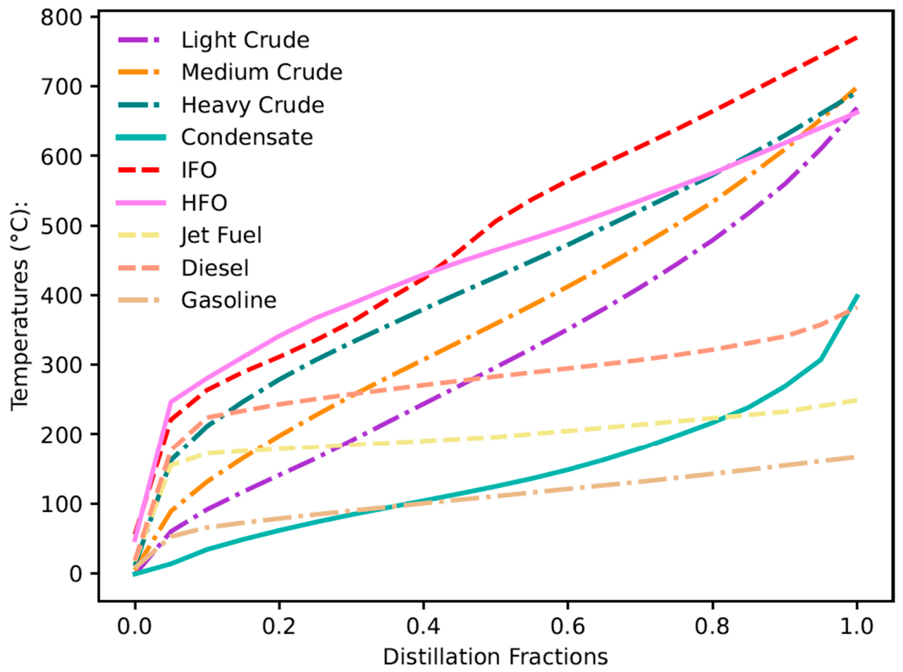
The average distillation curves for all the generic oil records are shown in Figure 6.

As the mean was calculated independently for each of 20 different mass fractions, individual statistics (e.g., standard deviation) have not been provided. To understand the spread of the distillation curves for each oil type, plots have been provided with the data set used to generate them for visual inspection in the Supplementary Materials (Figures S1–S9).

3.4. Impact on Modeling Results

As discussed in the introduction, one of the major goals of providing these “generic” oils is so users can gain an understanding of how a typical oil of a given type is likely to behave when released in the environment. If the user knows some detail about a product under consideration, they can select an oil record from the ADIOS Oil Database or any other source that better describes the specific product. But if all that is known is the broad category or type, a user may select a non-representative record, resulting in unrepresentative modeling results and expectations of how the oil might behave in the environment.

To demonstrate the different modeling results arising from a range of oils within a category, we performed a modeling exercise for a simple scenario for the weathering of a diesel fuel and medium crude oil. Oils used for this exercise can be found in

Table 11. Summary of oils used for modeling exercise.

Name	ADIOS ID	API	K. Visc. at 15 °C (cSt)	Frac. Evaporated (%)	Max Water Content (%)
Diesel Fuel Oil (Alaska)	AD02081	38.8	2.4	N/A	N/A
ULSFO Rotterdam Diesel	AD02608	28.2	13.5	N/A	N/A
Generic Diesel	GN00002	34.3	6.4	N/A	N/A
Green Canyon Block 200	EC00593	34.87	12.9	30.7	78
Neptune BHP [2009]	EC01459	21.49	434.9	0	81
Generic Medium Crude	GN00007	29.3	40.4	11.7	73.4

. The scenario is a release of 20,000 gal of product in open water with 10 knots of wind and a water temperature of 20 °C. The simulation was run for two days to reach a more-or-less steady state. These simulations were performed with the NOAA GNOME oil weathering model [15]. Other models should yield similar results.

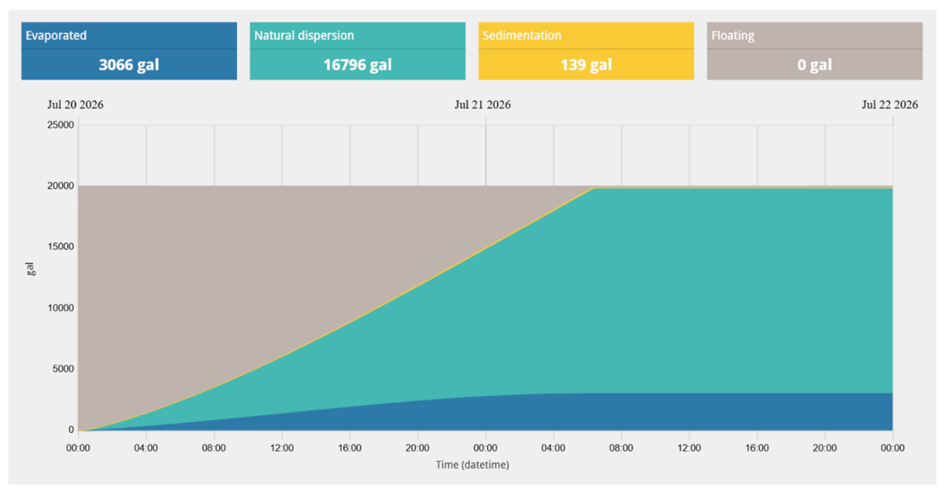
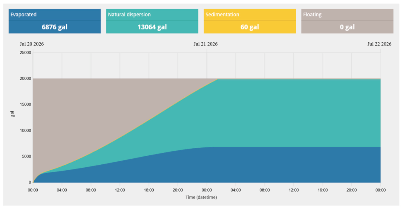
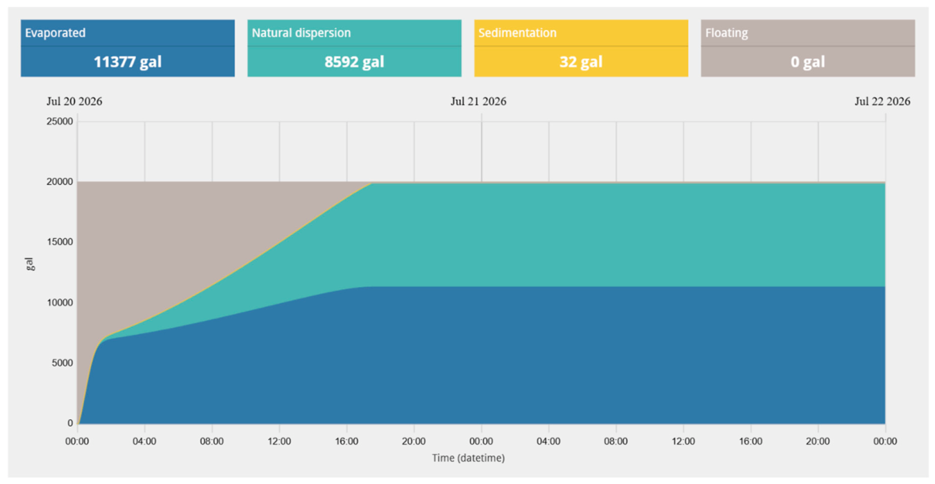
Figure 7, Figure 8 and Figure 9 show the results of the simulation for a diesel fuel on the lighter end of the range in the database (Diesel Fuel Oil (Alaska)), a heavier diesel fuel (ULSFO Rotterdam Diesel), and the generic diesel fuel. For the light fuel, approx. 57% of the oil evaporated, with the rest dispersing into the water column after about 18 h. With the heavier diesel fuel, only about 15% evaporated, with the rest ultimately dispersing after about 18 h. The generic oil resulted in approximately 34% evaporating, and the rest dispersing after about 24 h.

The ultimate persistence of a surface sheen between the three results is not very different, but the different amounts entering the water column due to dispersion could have a substantial impact on sub-surface biota. Responders could get a very different impression of the behavior of the oil depending on which record was chosen, and the generic record produced a result in between these two extremes.

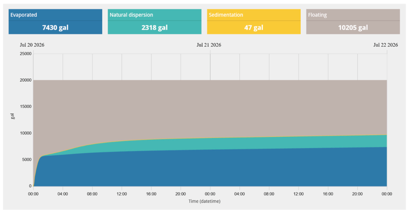
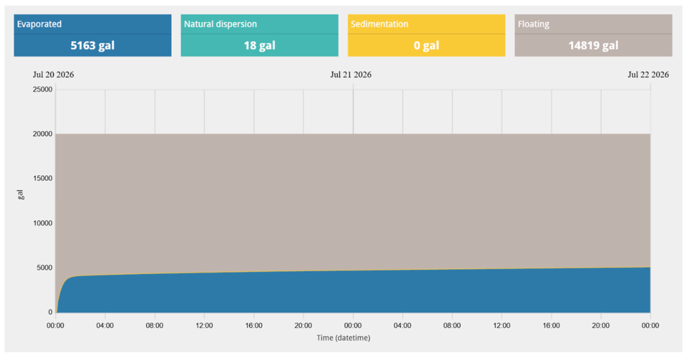
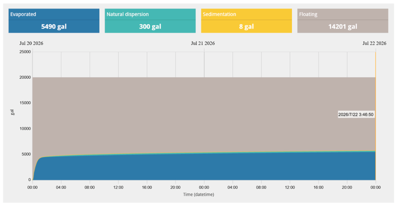
Figure 10, Figure 11 and Figure 12 show the results of the simulation for a medium crude on the lighter end of the density range for this category (Green Canyon Block 200), and one on the heavier end (Neptune BHP [2009]), as well as the Generic Medium Crude. For the lighter crude, approximately 37% of the oil evaporated, with about 12% dispersing and the rest remaining on the surface after two days. With the heavier crude, approximately 25% evaporated, virtually none dispersed, and the remaining oil was predicted to still be floating on the water surface after two days. The generic medium crude resulted in approximately 27% evaporating, less than 2% dispersing, and the remaining oil still floating after two days.

Note that in all three cases, an emulsion formed after some evaporation, greatly increasing the viscosity and preventing further dispersion. This indicates the wide range of results depending on exactly which medium crude is used in an assessment.

Examining the emulsification model further, the Green Canyon Block 200 (API: 34.87) starts to emulsify after about 6 h, and reaches a maximum water content of about 78%. The Neptune BHP (API: 21.49) starts to emulsify immediately, and reaches a maximum water content of 81%, while the Generic Medium Crude starts to emulsify after an hour or so, reaching a maximum water content of about 73.4%.

Note that emulsification is a very complex process, and the properties of the resulting emulsion depend on environmental conditions as well as the chemical composition of the oil. As a result, the maximum water content of an emulsion can vary widely, even among oils with similar API values. Furthermore, the emulsification model in GNOME is much simpler than what would realistically occur in the environment, and it is based on parameters measured in laboratory experiments.

In this case, the two example crudes had fairly high max water contents of around 80% (as determined with laboratory experiments), whereas the generic medium crude had a lower max water content (73.4%). The generic value is the middle of the range of max water content values for all the medium crudes in the database, and max water content does not necessarily correlate with density.

4. Conclusions

The final result of this project is a set of generic oil records that are useful to oil spill responders and modelers. Often in an oil spill response, or even for planning, the exact type of oil spilled is not known right away. Even when an exact type is known, there is often no assay of its physical properties available, particularly on an emergency response time scale. The records produced by this project provide a way for responders to quickly understand how the most common oil types are likely to behave in the environment, without requiring special expertise to choose an appropriate representative record from a database.

In addition to the generation of these records, this project served as an opportunity to look more closely at the data in the ADIOS Oil Database for consistency and accuracy. A number of records were corrected, and new ways to validate existing records were developed. These new methods will result in a more robust and complete database into the future.

The generic records are published on the ADIOS Oil Database website (search for “generic” or “GN” in the search bar, or select “Generic Oil” in the Labels dropdown list): https://adios.orr.noaa.gov.

From that site, the data can be viewed in an interactive web application or downloaded in a JSON format for use in other systems, including the NOAA GNOME oil weathering and trajectory modeling suite (https://gnome.orr.noaa.gov/).

Future work may involve expanding the generic oils collection to include generic oil records for certain types of Low Sulfur Fuel Oils (LSFOs), cold- and warm-weather diesels, and specific crude oils that have an abundance of measured data available, such as Louisiana Sweet crude.

5. Disclaimer

Although released by NOAA, the information in this paper does not reflect, represent, or form any part of the support of the policies of NOAA or the Department of Commerce. Further, release by NOAA does not imply that NOAA or the Department of Commerce agree with the information contained herein.

References

1. National Oceanic and Atmospheric Administration Office of Response and Restoration. The ADIOS Oil Database. Available online: https://adios.orr.noaa.gov (accessed on 22 December 2025).
2. National Oceanic and Atmospheric Administration Office of Response and Restoration. ADIOS Oil Database Data Used to Generate Generic Oils [Data Set]. Available online: https://github.com/NOAA-ORR-ERD/noaa-oil-data/releases/tag/2025-12-22 (accessed on 22 December 2025).
3. Lehr, W.J. Review of the Modeling Procedures for Oil Spill Weathering Behavior. In Oil Spill Modelling and Processes; Brebbia, C.A., Ed.; WIT Press: Boston, MA, USA, 2001; pp. 51–90. [Google Scholar]
4. Spaulding, M.L. State of the Art Review and Future Directions in Oil Spill Modeling. Mar. Pollut. Bull. 2017, 115, 7–19. [Google Scholar] [CrossRef] [PubMed]
5. Geng, X.; Barker, C.H.; MacFadyen, A.; Boufadel, M.C.; Thrift-Viveros, D.L.; Jones, R.K.; O’Connor, C.; Lee, K.A. Generic Approach to Construct Pseudo Components for Oil Weathering Models. J. Hazard. Mater. 2023, 459, 132160. [Google Scholar] [CrossRef] [PubMed]
6. Fingas, M. (Ed.) Charter 8: Water-in-oil Emulsion Formation. In Handbook of Oil Spill Science and Technology; John Wiley and Sons Inc.: New York, NY, USA, 2015; pp. 225–270. [Google Scholar]
7. Fingas, M.F.; Fieldhouse, B.G. Water-in-oil Emulsions: Formation and Prediction. In Proceedings of the Thirty-Fourth AMOP Technical Seminar on Environmental Contamination and Response; Environment Canada: Ottawa, ON, Canada, 2011; pp. 460–510. [Google Scholar]
8. Lehr, W.; Jones, R.; Evans, M.; Simecek-Beatty, D.; Overstreet, R. Revisions of the ADIOS oil spill model. Environ. Model. Softw. 2002, 17, 191–199. [Google Scholar] [CrossRef]
9. Jones, R.K. A simplified pseudo–component oil evaporation model. In Proceedings of the Twentieth Arctic and Marine Oilspill Program (AMOP) Technical Seminar; Environment Canada, Emergencies Science Division: Ottawa, ON, Canada, 1997; pp. 43–61. [Google Scholar]
10. United States Coast Guard National Response Center. Initial Reports of Pollution Incidents in the United States, 2015–2019 Reports and 2020–2024 Reports. Available online: https://nrc.uscg.mil/ (accessed on 24 January 2025).
11. Berger, S.; Chever, F.; Iversen, T.; Legrand, S.; Savic, J.; Zammit, M.; Holbu, J.W.; Dolva, H.; Frogner, I.A.; Frost, B.R. Response to LSFO spills–results from the IMAROS-project. In Proceedings of the International Oil Spill Conference, New Orleans, LA, USA, 13–16 May 2024; Volume 2024. [Google Scholar]
12. Gilbert, T. VLSFO Study Report 2022 for Australian Maritime Safety Authority, AMSA; Reef Ecologic: Townsville, Australia, 2022. [Google Scholar]
13. Raymond, M.; Leffler, W. Oil and Gas Production in Nontechnical Language, 2nd ed.; PennWell Books: Tulsa, OK, USA, 2017. [Google Scholar]
14. US Energy Information Agency. Glossary. Available online: https://www.eia.gov/tools/glossary/index.php (accessed on 3 March 2021).[Green Version]
15. Barker, C.H.; Jones, R.K.; Lehr, W.J.; MacFadyen, A.; O’Connor, C.; Makela, J.; Hennen, J.; Geng, X. GNOME Technical Documentation (2026); NOAA Emergency Response Division: Seattle, WA, USA.
16. Box, G.E.P.; Cox, D.R. An Analysis of Transformation. J. R. Stat. Soc. B 1964, 26, 211–252. [Google Scholar] [CrossRef]
Figure 1. Histogram of density (in kg/m3) at 288 K (15 °C) of light crudes plotted against the number of samples. The data are fairly normally distributed, with mild skewness of (0.0384)—not enough to require a transform to determine the typical density.
Jmse 14 01450 g001
Figure 2. Histogram of 406 kinematic viscosity values for all the light crudes at 288 K (15 °C) in the database. The green line is at the mean value, with the red lines at the mean plus and minus one standard deviation.
Jmse 14 01450 g002
Figure 3. Histogram of kinematic viscosity values for light crudes, zoomed in on the region where most of the data are. The green line is at the mean value, with the red lines at the mean plus and minus one standard deviation.
Jmse 14 01450 g003
Figure 4. Histogram of the kinematic viscosity of light crudes at 288 K (15 °C) after Box–Cox transformation. The green line is at the mean value, with the red lines at the mean plus and minus one standard deviation.
Jmse 14 01450 g004
Figure 5. Histogram of kinematic viscosity values for light crudes, focused on the region where most of the data are. The green line is at the mean value reverse-transformed, with the red lines at the mean plus and minus one reverse-transformed standard deviation.
Jmse 14 01450 g005
Figure 6. Distillation curves of generic oil records produced for nine oil types.
Jmse 14 01450 g006
Figure 7. GNOME weathering model results for the Diesel Fuel Oil (Alaska).
Jmse 14 01450 g007
Figure 8. GNOME weathering model results for the ULSFO Rotterdam Diesel fuel.
Jmse 14 01450 g008
Figure 9. GNOME weathering model results for the Generic Diesel fuel.
Jmse 14 01450 g009
Figure 10. GNOME weathering model results for the Green Canyon Block 200 crude oil.
Jmse 14 01450 g010
Figure 11. GNOME weathering model results for the Neptune BHP [2009] crude oil.
Jmse 14 01450 g011
Figure 12. GNOME weathering model results for the Generic Medium Crude.
Jmse 14 01450 g012