High-SNR Balanced Field Electromagnetic Detection Method for Subsea Pipeline Cracks Based on Sampling Optimization

Abstract

During crack detection in subsea oil and gas pipelines under strong-noise conditions, balanced field electromagnetic technique (BFET) exhibits limited capability to reconstruct the amplitude and phase features of crack signals and produces a relatively low signal-to-noise ratio (SNR). To address these limitations, a high-SNR detection method based on the joint optimization of sampling parameters and reference accuracy is proposed. A finite-element model of the balanced field electromagnetic sensor was established. The time-domain voltage signal of the crack detection signal and its amplitude–phase features were then obtained. By fitting the crack detection signals and introducing Gaussian white noise and quantization noise, the effects of different sampling frequencies, sampling accuracies, and reference accuracies on the reconstruction accuracy of the amplitude–phase features and on the SNR of the detection signals were systematically investigated. The experimental results show that, at an excitation frequency of 1 kHz, a sampling frequency of 64 kHz, and both a sampling accuracy and reference accuracy of 16 bits, the amplitude and phase errors of the crack detection signals are significantly reduced, while the SNR exceeds 31.74 dB. The proposed method provides a reference for evaluating the influence of sampling parameters and reference accuracy on the detection SNR and the reconstruction accuracy of amplitude–phase features.

1. Introduction

Subsea oil and gas pipelines serve as essential energy transportation channels connecting abundant offshore hydrocarbon resources with onshore storage and transportation terminals, and they constitute critical infrastructure for the long-distance transmission of offshore oil and gas resources. During long-term service, subsea oil and gas pipelines are exposed to harsh marine environments characterized by high pressure, low temperature, and strong corrosion, while also being affected by seabed movement and external impact loads. As a result, defects such as corrosion, fatigue damage, and cracks are prone to occurring in the pipe body, leading to a reduction in pipeline load-bearing capacity and, in severe cases, subsea oil and gas leakage, explosions, and marine ecological pollution [1]. Therefore, crack defect detection in subsea oil and gas pipelines is of great significance for safeguarding the marine environment and ensuring the safety of oil and gas transportation.

For the detection of defects in subsea oil and gas pipelines, manual inspection and maintenance are not only highly challenging but also associated with high risks and low efficiency, because pipelines are typically deployed in seabed environments for long-term service. Therefore, pipeline in-line inspection has become an important approach for subsea pipeline inspection, mainly including magnetic flux leakage testing, ultrasonic testing, and eddy current testing [2]. Magnetic flux leakage testing is sensitive to surface and buried volumetric defects and is suitable for rapid, large-area pipeline inspection. However, its sensitivity to linear defects, such as cracks, remains relatively low [3,4,5]. Ultrasonic testing is sensitive to internal cracks and wall-thickness variations in pipelines, but it imposes relatively high requirements on the surface finish of the inspected components. When ultrasonic waves propagate in inhomogeneous or highly attenuating materials, their energy is attenuated and penetration capability decreases, resulting in a degraded signal-to-noise ratio. In addition, conventional piezoelectric ultrasonic testing requires a couplant to ensure effective acoustic coupling with the pipe surface, which limits its applicability to gas pipelines. Although electromagnetic ultrasonic testing does not require a couplant, it is only highly sensitive to cracks with specific orientations [6,7,8]. As a non-contact and rapid inspection method, eddy current testing has been extensively utilized for crack detection. However, its crack detection sensitivity is limited to some extent by the skin effect and lift-off effect [9,10,11].

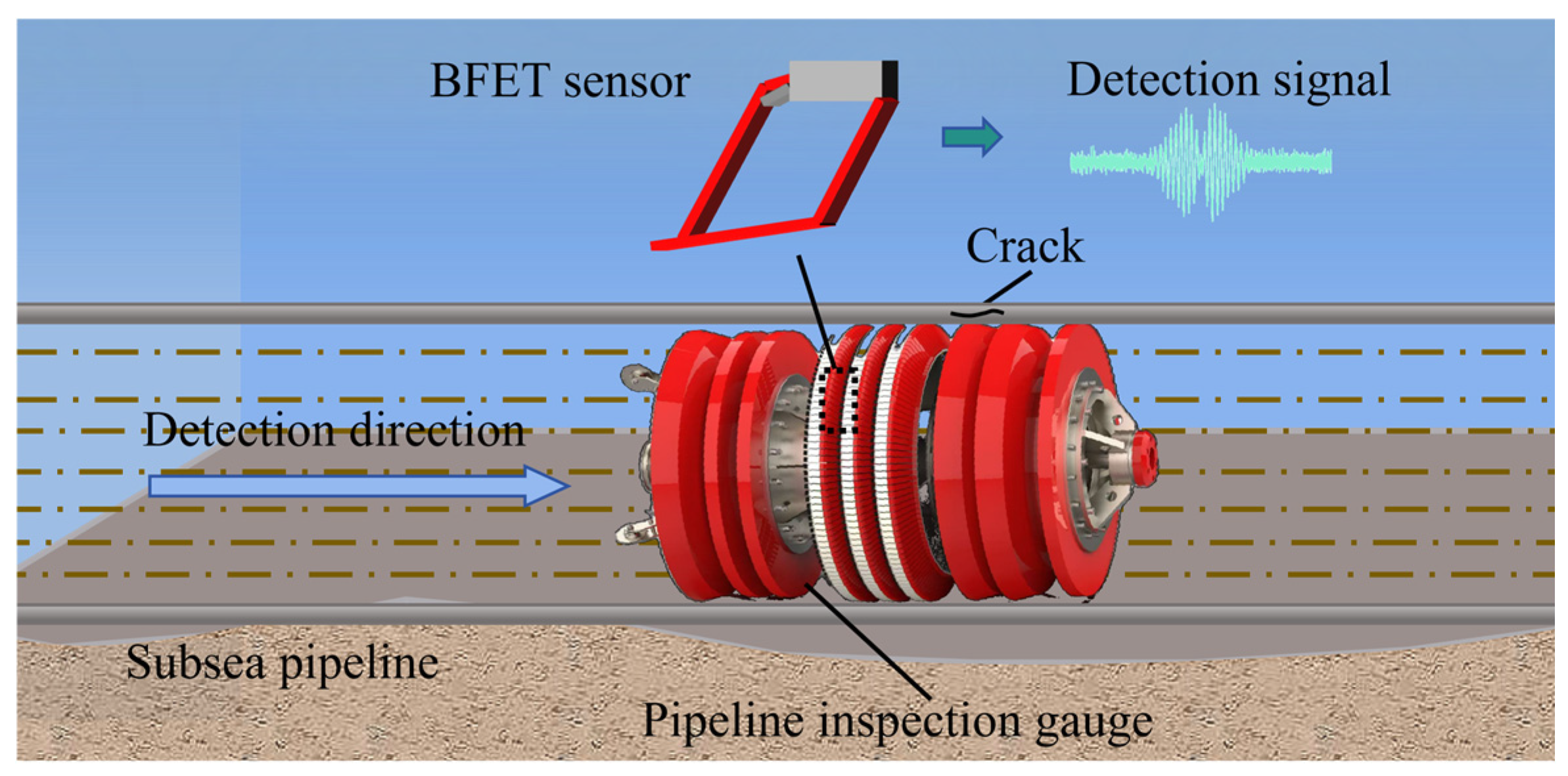
The BFET can simultaneously perceive variations in the eddy current field and the magnetic flux leakage field. It is immune to the lift-off effect, exhibits high sensitivity to cracks, and provides effective detection capability for cracks in arbitrary orientations in pipelines [12,13], as shown in Figure 1. However, in practical inspection, substantial environmental noise and electromagnetic interference are commonly present. During signal acquisition, such noise may overwhelm the weak crack detection signals, thereby reducing the detection signal-to-noise ratio. To improve the SNR of crack detection under strong-noise conditions, Z. F. Zhang et al. [14] proposed a method incorporating adaptive noise cancelation in the fractional domain, signal enhancement, and multi-scale feature extraction, achieving a recognition accuracy of up to 98.22% under strong background noise. To address signal aliasing and low SNR in pipeline inspection, W. Li et al. [15] proposed a method combining three-probe differential signal enhancement with characteristic coefficients, which improved the signal-to-noise ratio (SNR) SNR from −15 dB to 2.4 dB and limited the quantitative error of crack size to within 8.75%. J. L. Li et al. [16] proposed an improved minimum entropy deconvolution (MED)-based method of fault feature extraction from signals that could extract defect features from signals acquired in high-noise environments, thereby substantially improving the SNR. J. S. Bai et al. [17] addressed the issue that transient electromagnetic weak signals are easily submerged in noise, and a multi-scale combined differential product morphological filtering method was proposed. By combining multi-scale feature enhancement with morphological denoising, the proposed method effectively improves the extraction capability of weak transient signals. W. X. Zheng et al. [13,18] proposed a same-frequency excitation method for eliminating frequency-difference noise. By adopting a unified clock excitation scheme for all channels and developing a same-frequency excitation system, their method eliminated frequency-difference noise at the source end and achieved a high SNR. The above studies effectively improved the SNR by enhancing signal processing algorithms or optimizing excitation strategies. However, for the entire crack detection process, the acquisition of high-quality original data is also of critical importance.

To obtain high-quality original data, the sampling parameters and reference accuracy must be carefully selected during crack-signal acquisition, as they directly affect the quality of the acquired signal and, consequently, the overall signal-to-noise ratio (SNR) of the system. S. H. Huang et al. [19] introduced a 24-bit high-resolution analog-to-digital converter and strictly matched the sampling frequency with the sampling accuracy, thereby eliminating the need for complex analog balancing circuits, significantly reducing system noise at the source, and significantly improving the SNR of defect detection. Z. T. Xia et al. [20] emphasized that, in strong-noise environments, in addition to the back-end discrete wavelet transform algorithm, the use of a high-accuracy 24-bit ADC and a sampling frequency of 128 kHz at the front end provides the physical basis for high-quality acquisition of weak defect signals and significant improvement in the SNR. C. Zhang et al. [21] proposed a joint denoising approach combining intelligently optimized decomposition with normalized least-mean-square filtering, demonstrating strong adaptability to non-stationary weak signals. They further reported that, under low-sampling-frequency conditions, both the convergence rate of the steady-state response and the fidelity of the acquired signal are markedly reduced. These studies collectively demonstrate the critical role of sampling parameters in signal acquisition. However, to the best of our knowledge, existing publicly available studies have not yet clarified how sampling parameters affect the reconstruction accuracy of amplitude–phase features in crack detection signals or the signal-to-noise ratio of such signals.

To improve the detection performance of the balanced field electromagnetic technique in practical pipeline in-line inspection applications, the focus of this paper is the data acquisition phase of the BFET. A high-SNR detection method based on sampling optimization is proposed. This method aims to clarify the effects of signal acquisition and demodulation parameters on the reconstruction accuracy of the amplitude–phase features of crack detection signals, as well as on the SNR of the detection signals. The principle of the BFET was investigated, and a signal feature sampling analysis algorithm was established. The effects of sampling frequency, sampling accuracy, and reference accuracy on the reconstruction accuracy of crack amplitude–phase features and the detection SNR were analyzed. Furthermore, the proposed method was experimentally validated.

2. Detection Principle of the BFET

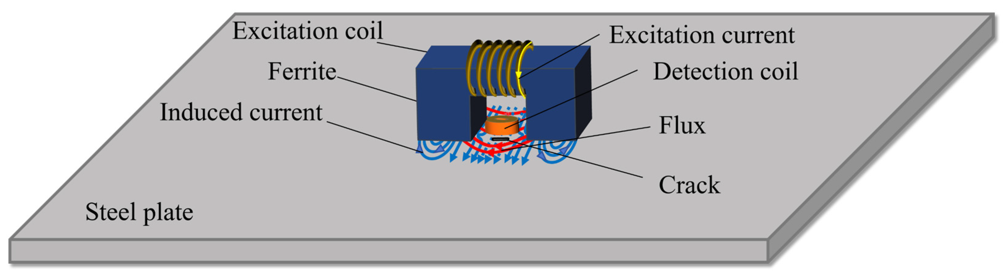
The balanced field electromagnetic technique integrates alternating-current electromagnetic testing with alternating-current magnetic flux leakage testing and employs alternating-current excitation. Pipeline defects are detected by measuring variations in the spatial magnetic field caused by changes in the eddy current and magnetic flux distributions on the surface of the component under inspection, using a pair of mutually orthogonal and geometrically symmetric coils. When an alternating current is supplied to the excitation coil, both an alternating magnetic field and an eddy current field are induced on the pipeline surface. Instead of relying solely on either magnetic flux leakage or eddy currents, this technique detects defect-induced electromagnetic variations under the combined action of both fields. Figure 2 presents a schematic illustration of the BFET sensor.

Under an ideal balanced condition, when an alternating current is applied to the excitation coil, the geometrically symmetric arrangement of the excitation and detection coils ensures that the magnetic field coupled to the detection coil remains balanced over a defect-free region of the steel plate. Consequently, no voltage is induced in the detection coil. Once a crack is present in the tested specimen, magnetic flux leakage occurs at the specimen–air interface and interacts with the magnetic field lines generated by the excitation coil to form a closed magnetic path. At the same time, the time-varying magnetic field induces eddy currents on the specimen surface. These eddy currents cause electromagnetic field distortion near both crack tips and disturb the original field equilibrium. The detection coil captures this distortion, thereby enabling crack detection [22].

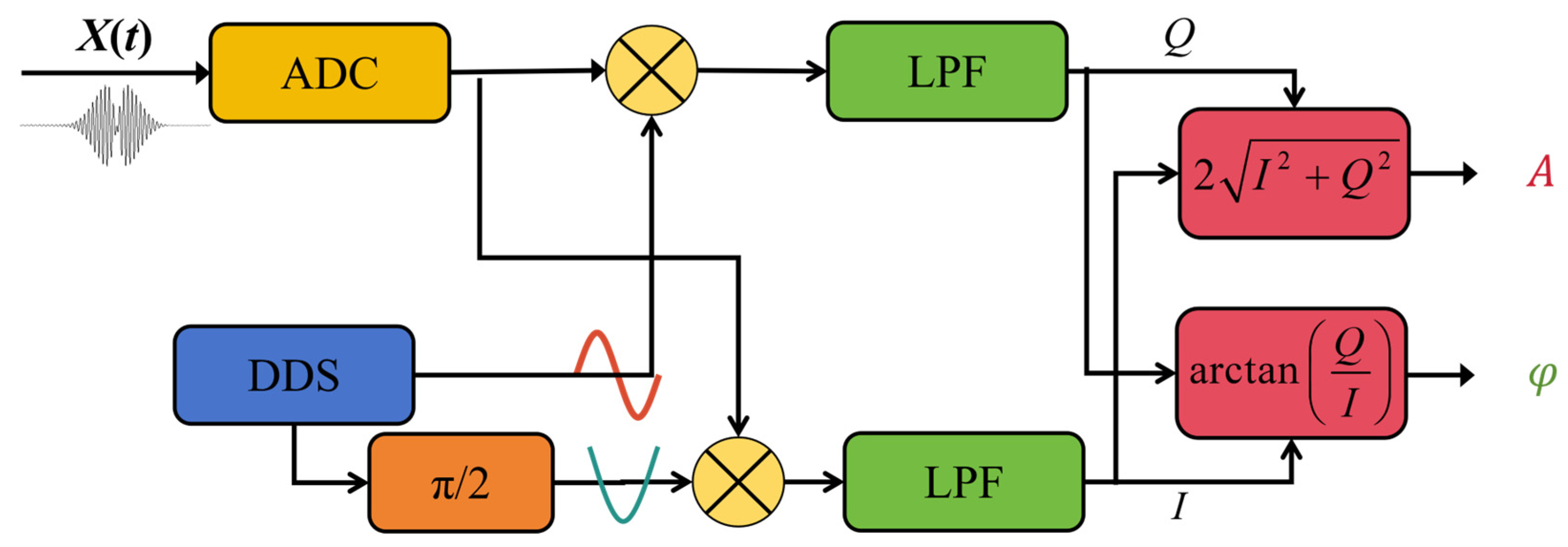
To obtain the amplitude–phase features of crack detection signals from the signal envelope, this study adopted the processing procedure illustrated in Figure 3.

After the BFET crack detection signal X(t) is input, the signal generator simultaneously generates two mutually orthogonal digital reference signals, each with a peak amplitude of 1, and each reference signal is multiplied by the input balanced field electromagnetic crack detection signal. The two resulting signals then pass through a fourth-order digital Butterworth low-pass filter with a cutoff frequency of 100 Hz and an extremely narrow bandwidth to remove high-frequency components and random noise whose frequency differs from that of the reference signals, thereby outputting the in-phase component I and quadrature component Q. The measured signal amplitude A and phase $\phi$ are then obtained using Equations (1) and (2), respectively.

$$A=2\sqrt{I^2+Q^2}$$

(1)

$$\phi =\arctan \left({\displaystyle \frac{Q}{I}}\right)$$

(2)

3. Finite-Element Simulation and Signal Feature Sampling Analysis Algorithm

To investigate the effects of sampling parameters during the data acquisition stage on the amplitude and phase feature errors as well as the signal-to-noise ratio (SNR) of crack inspection signals, a three-dimensional finite-element model of a balanced field electromagnetic sensor for crack detection was established. The output voltage of the detection coil was extracted as the original inspection signal for subsequent analysis. A signal feature sampling and analysis algorithm was then developed to evaluate the effects of the sampling frequency, sampling accuracy, and reference accuracy on the reconstruction accuracy of the amplitude and phase features of the crack inspection signal.

3.1. Finite-Element Simulation

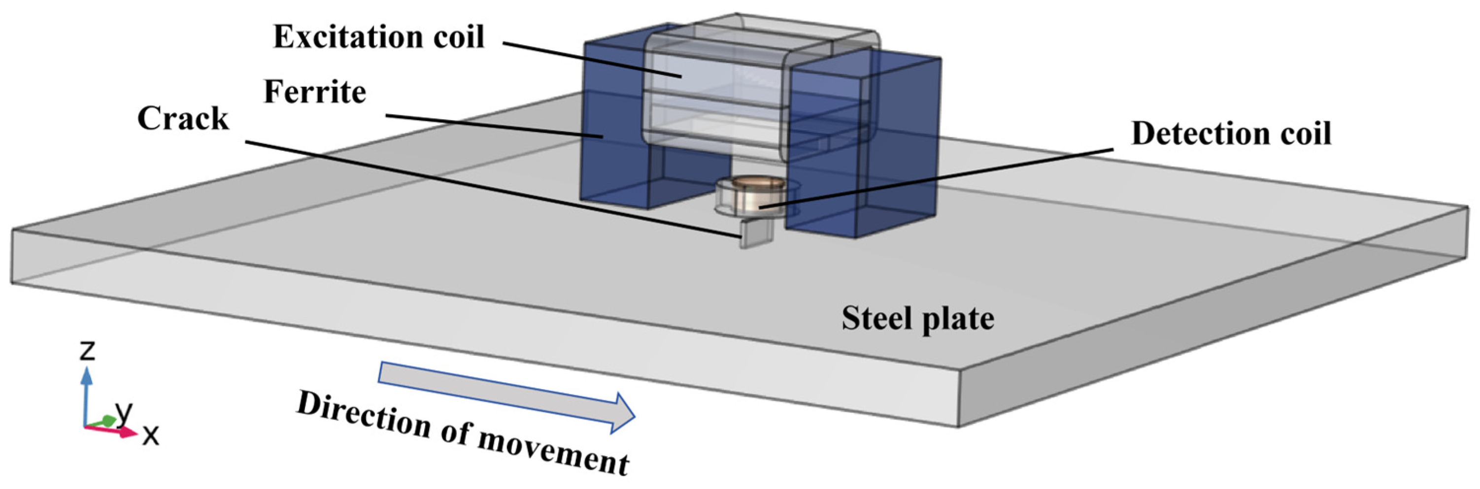
To provide standardized, noise-free original crack inspection signals for subsequent signal feature extraction and analysis, a three-dimensional finite-element electromagnetic model was established. As illustrated in Figure 4, the model consists of a balanced field electromagnetic sensor and a steel plate. The balanced field electromagnetic sensor comprises a ferrite, an excitation coil, a detection coil, and an air domain. The geometric dimensions of the model and the corresponding material properties are summarized in

Table 1. Dimensions and parameters of each component in the sensor simulation model.

Component	Dimensions (mm) (Length × Width × Height)	Relative Permeability	Electrical Conductivity (S/m)
ferrite	60 × 30 × 30	5000	0.001
steel plate	200 × 100 × 10	1000	1.6 × 106
coil	(ID × OD) 15 × 30	1	6 × 107
air domain	400 × 400 × 400	1	0

.

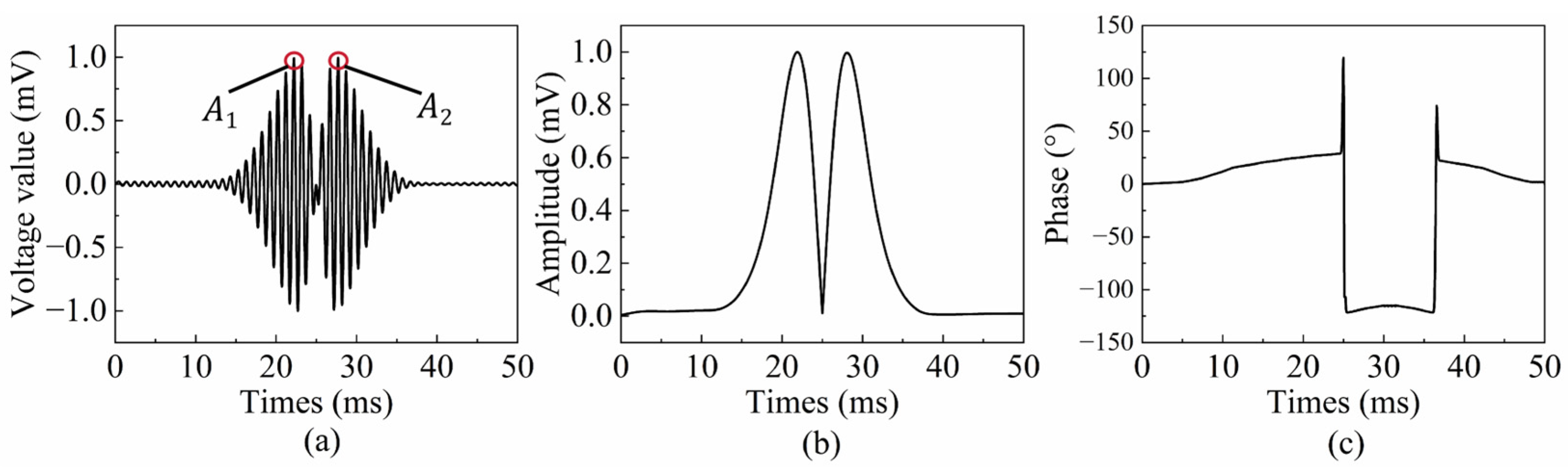
In Figure 4, the air domain is hidden. The air domain was hidden for clarity. The crack was oriented perpendicular to the sensor scanning direction and had a length of 40 mm, a width of 0.3 mm, and a depth of 3 mm. The excitation coil and detection coil were assigned copper as their material, with 1000 and 500 turns, respectively. The magnetic field interface was selected as the physical field, and the entire model satisfied the boundary conditions governed by Ampere’s law. To simulate the moving scanning process, a 1 kHz sinusoidal alternating current was applied to the excitation coil. The sensor lift-off height was set to 1 mm to ensure the entire crack passed beneath the detection sensor. The center of the steel plate surface was defined as the coordinate origin, and the sensor was scanned along the X-axis direction shown in Figure 4. The starting and ending positions were set to (−30, 0, 0) and (30, 0, 0), respectively. The movement step size of the sensor was set to 1 mm. Once the monitored quantities had stabilized during the final stages of iteration, the output voltage of the detection coil was extracted as the crack detection signal and processed according to the procedure shown in Figure 3 to obtain the in-phase and quadrature components. The amplitude and phase of the original detection signal were calculated using Equations (1) and (2), respectively, as shown in Figure 5. To facilitate the subsequent analysis of the reconstruction accuracy of the amplitude–phase features of the original crack detection signal, the two envelope peaks of the crack detection signal in Figure 5a are denoted as A₁ and A₂.

3.2. Effects of Sampling Parameters on Reconstruction Accuracy of Crack Detection Signal Amplitude–Phase Features

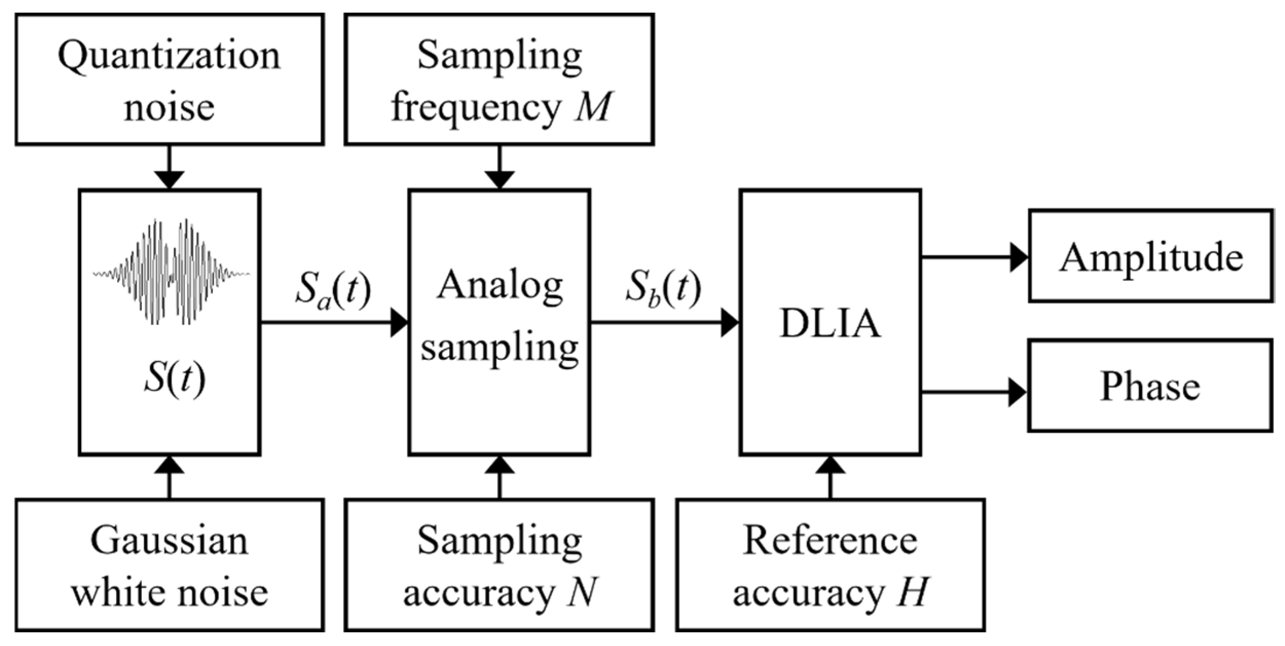
To investigate the effects of sampling frequency, sampling accuracy, and reference accuracy on the reconstruction accuracy of the amplitude–phase features of crack detection signals and on the SNR of detection signals, a signal feature sampling analysis algorithm was designed, and simulations were performed using numerical simulation software. The workflow is shown in Figure 6.

The crack detection signal shown in Figure 5a was used as the data source S(t) for executing the algorithm shown in Figure 6. To simulate random electromagnetic interference in practical engineering environments, Gaussian white noise was added to S(t). In addition, approximately uniformly distributed quantization noise was introduced to model the thermal noise in the sensor circuit. Different combinations of sampling frequency M and sampling accuracy N were then set to perform simulated sampling on S_a(t). Meanwhile, to investigate the influence of quantization error on the reconstruction accuracy of the amplitude–phase features of crack detection signals, the reference accuracy H was defined. This parameter denotes the number of quantization bits of the reference signal in the digital lock-in amplifier (DLIA) and is used to evaluate the quantization resolution of the reference signal. Finally, the simulated sampled signal S_b(t) shown in Figure 6 was processed using the algorithm shown in Figure 3, and the amplitude and phase of the crack detection signal were output. To isolate the effects of the individual parameters, all calculations were performed using the same noise-free signal and identical realizations of Gaussian white noise and quantization noise. However, the mean and standard deviation of the results across different random-noise realizations were not evaluated.

3.2.1. Effects of Sampling Frequency on the Amplitude–Phase Feature Errors of Detection Signals

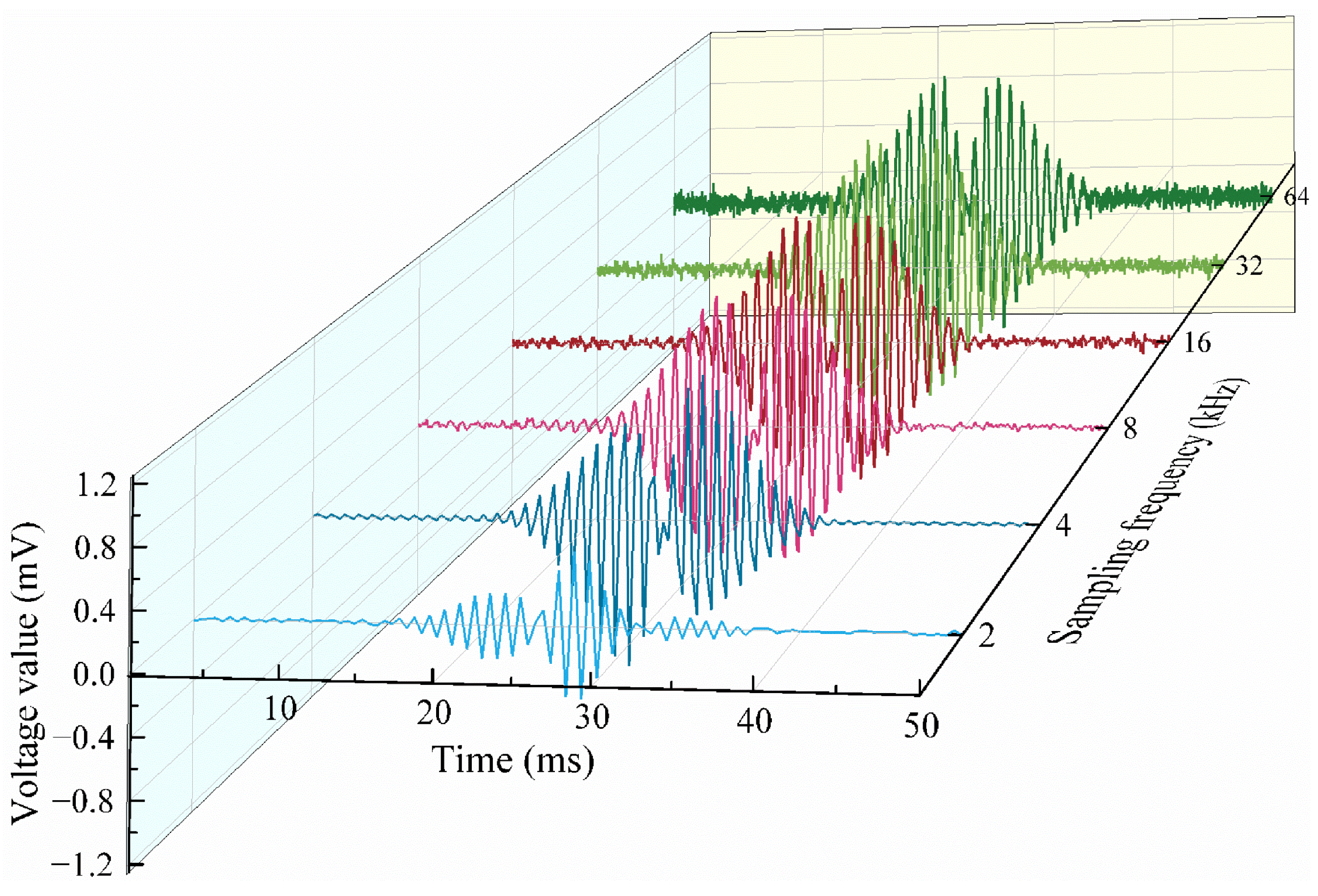
To investigate the influence of different sampling frequencies on the reconstruction accuracy of the amplitude–phase features of crack detection signals, the sampling accuracy N was fixed at 16 bits. According to the algorithmic workflow shown in Figure 6, the sampling frequency M was set to 2, 4, 8, 16, 32, and 64 kHz, respectively. The simulated sampled crack detection signals S_b(t) obtained under these sampling frequencies are shown in Figure 7.

As shown in Figure 7, the simulated sampled signal S_b(t) maintains a waveform consistent with that of the crack detection signal in Figure 5. At a sampling frequency of 2 kHz, the sampling points of the detection signal are excessively sparse, resulting in a coarse and discontinuous waveform. Given an excitation frequency of 1 kHz, a sampling frequency of 4 kHz provides only four sampling points per excitation cycle, which remains insufficient to accurately characterize the waveform details and amplitude–phase features. After applying the processing procedure shown in Figure 3, the amplitude and phase information of the crack detection signal cannot be accurately reconstructed. As the sampling frequency increases from 8 to 64 kHz, the sampling points become progressively denser. This not only preserves the overall variation trend of the envelope but also ensures that the detailed components of the crack signal are retained. Therefore, in the subsequent simulations, only sampling frequencies M of 8, 16, 32, and 64 kHz were selected for analysis.

To further analyze the reconstruction accuracy of the amplitude–phase features at different sampling frequencies, the detection signals in Figure 7 were processed using the algorithm shown in Figure 3. Subsequently, the amplitude and phase information reflecting the crack feature was extracted. Following the example method shown in Figure 5a, the two envelope peaks, A₁ and A₂, were extracted from the detection signals sampled at 8, 16, 32, and 64 kHz in Figure 7. The amplitude error E_Ak and phase error $E_{\phi }$ of each signal were then calculated using Equations (3) and (4), respectively.

$$E_{A_k}=\left|{\displaystyle \frac{P_n-P_{t_k}}{P_k}}\right|\times 100\%,\hspace{0.33em}\hspace{0.33em}(k=1,\hspace{0.33em}2)$$

(3)

$$E_{\phi }=\left|{\phi }_n-{\phi }_t\right|$$

(4)

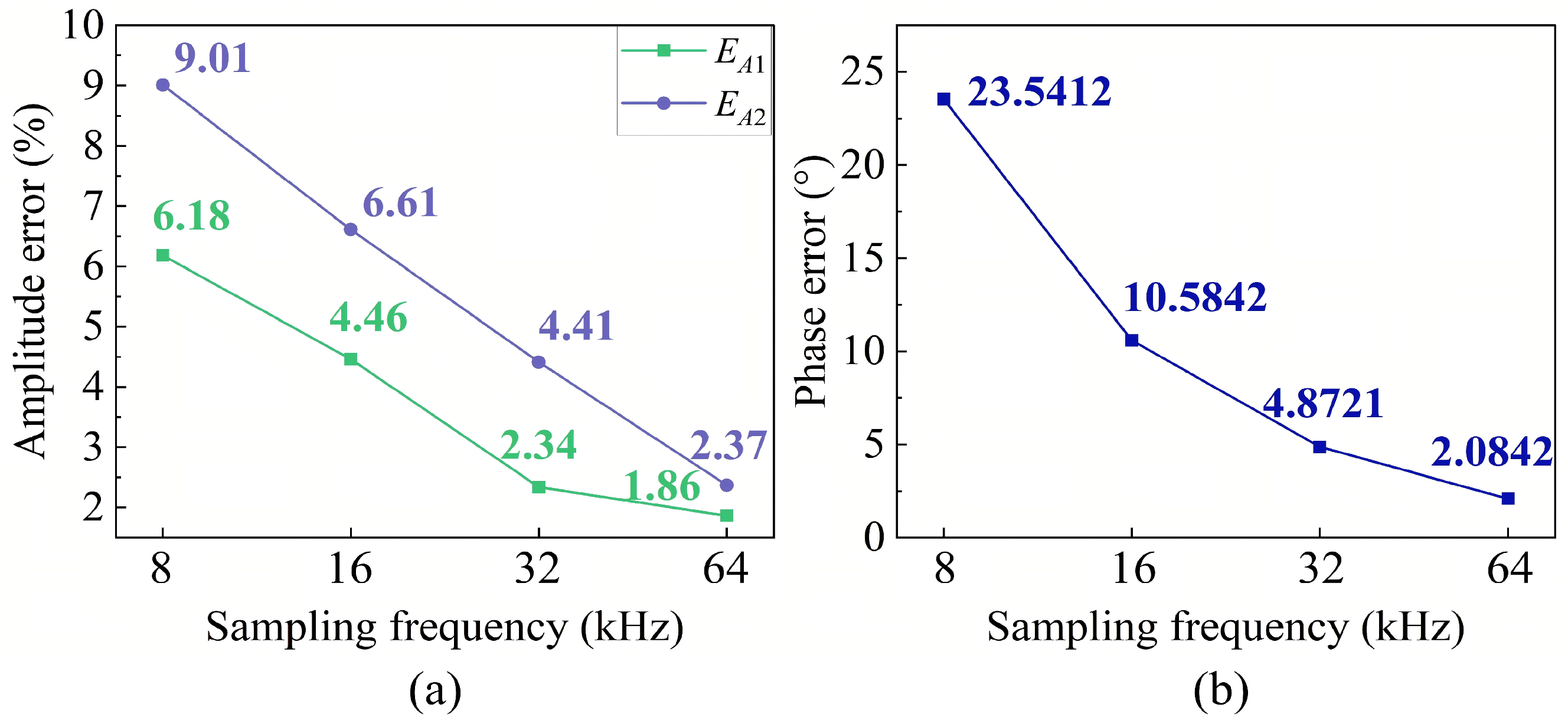
In Equation (3), P_n denotes the two envelope peaks of the detection signals at different sampling frequencies in Figure 7, where n (ranging from 1 to 4) corresponds to sampling frequencies of 8, 16, 32, and 64 kHz, respectively. P_tk denotes the envelope peak in Figure 5a, where (k = 1, 2). In Equation (4), ${\phi }_n$ denotes the phase information of the detection signal at each sampling frequency in Figure 7 calculated using the procedure shown in Figure 3. ${\phi }_t$ represents the simulated phase of the detection signal obtained from Figure 5c. The calculated amplitude error of the first envelope peak E_A1, the amplitude error of the second envelope peak E_A2, and the phase error of the detection signal $E_{\phi }$ at sampling frequencies of 8, 16, 32, and 64 kHz are shown in Figure 8.

As shown in Figure 8, the amplitude errors of the two envelope peaks and the phase error of the signal decrease within the sampling frequency range of 8–64 kHz. Higher sampling frequencies result in smaller errors. When the sampling frequency reaches 32 kHz or higher, the variation trends of the amplitude and phase errors become less pronounced. Within the range of sampling frequencies investigated in this study, at a sampling frequency of 64 kHz, the amplitude errors of the two envelope peaks, E_A1 and E_A2, reach their minimum values of 2.37% and 1.86%, respectively. The phase error $E_{\phi }$ also reaches its minimum value of 2.084°. These results indicate that a sampling frequency of 64 kHz can effectively reconstruct the amplitude–phase features of crack detection signals. Therefore, in balanced field electromagnetic crack detection, setting the sampling frequency to 64 kHz is appropriate for effective signal feature analysis and quantitative crack evaluation.

3.2.2. Effects of Sampling Accuracy on the Amplitude–Phase Feature Errors of Detection Signals

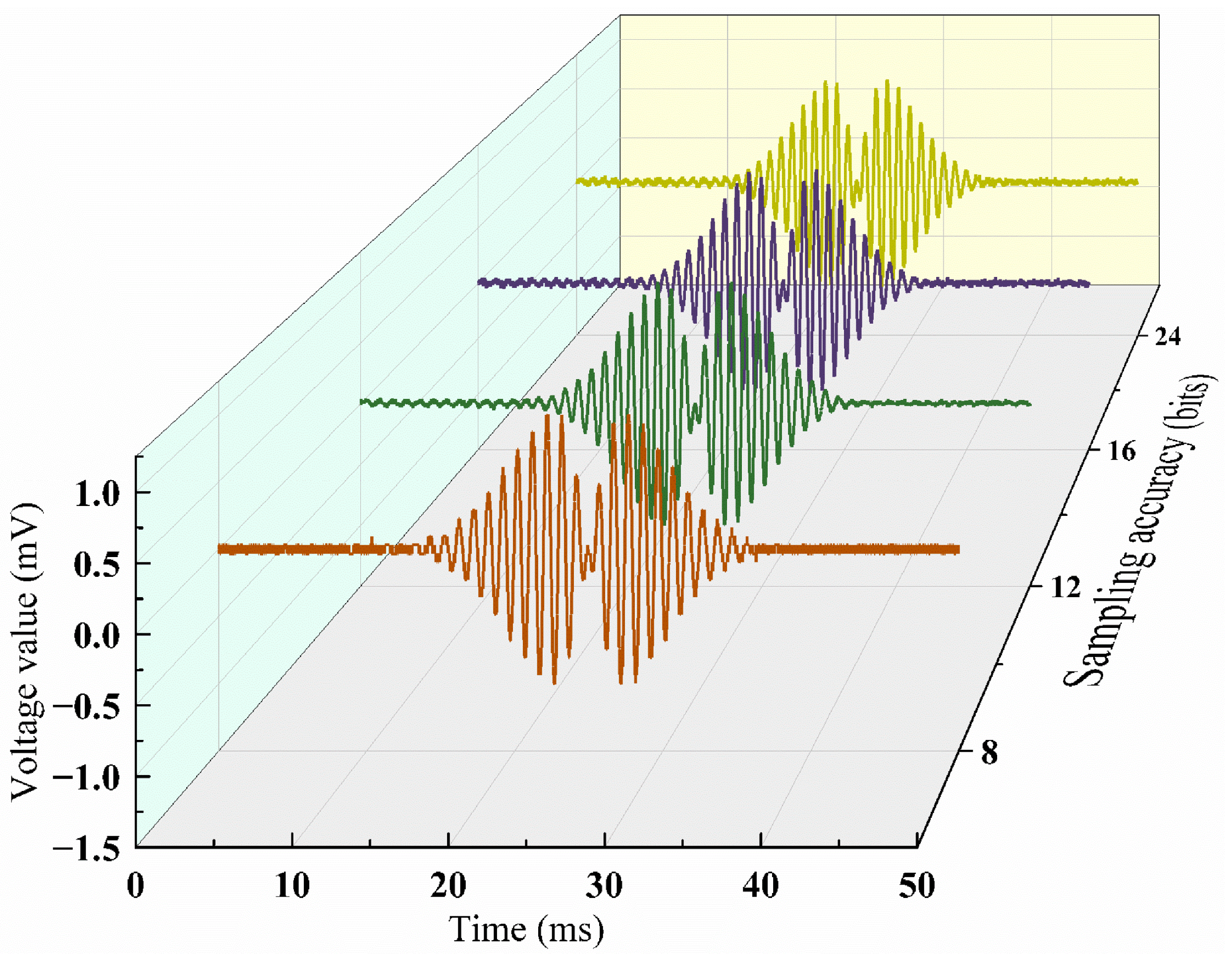
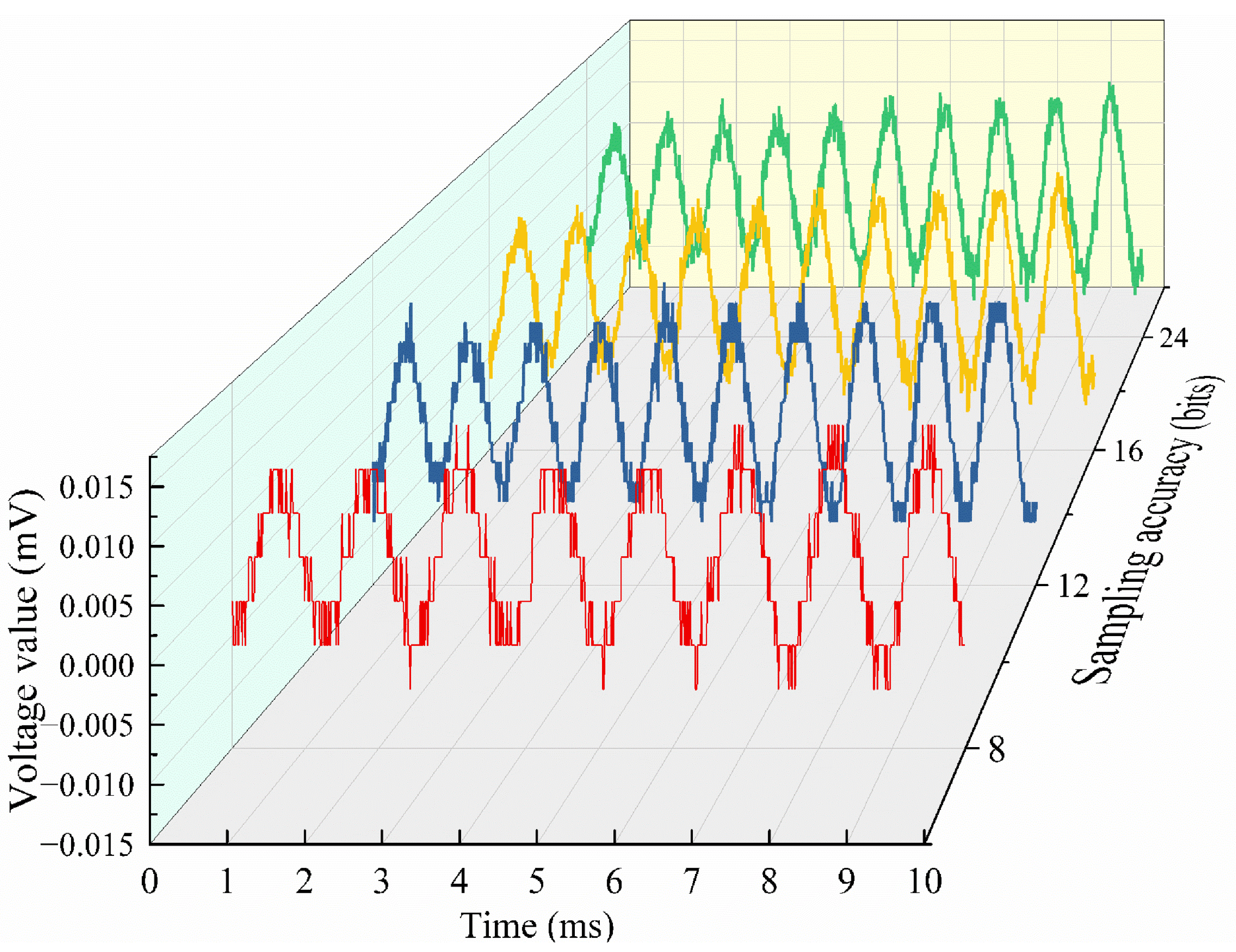
To analyze the variation trends in amplitude–phase feature errors in crack detection signals under different sampling accuracies, the signals were further processed. As described in Section 3.2.1, when the sampling frequency was 64 kHz, the signal processed according to Figure 6 exhibited the minimum amplitude and phase errors. Therefore, the sampling frequency was fixed at 64 kHz, and the sampling accuracy N in Figure 6 was set to 8, 12, 16, and 24 bits, respectively. The simulated sampled signals S_b(t) obtained under these conditions are shown in Figure 9.

As shown in Figure 9, when the sampling frequency is 64 kHz and the sampling accuracy is 8 bits, the signal exhibits pronounced step-like fluctuations and a serrated feature. As the sampling accuracy increases to 16 and 24 bits, the serrated features disappear. Consequently, the reconstruction accuracy of the crack detection signal is significantly improved, and its detailed components are preserved.

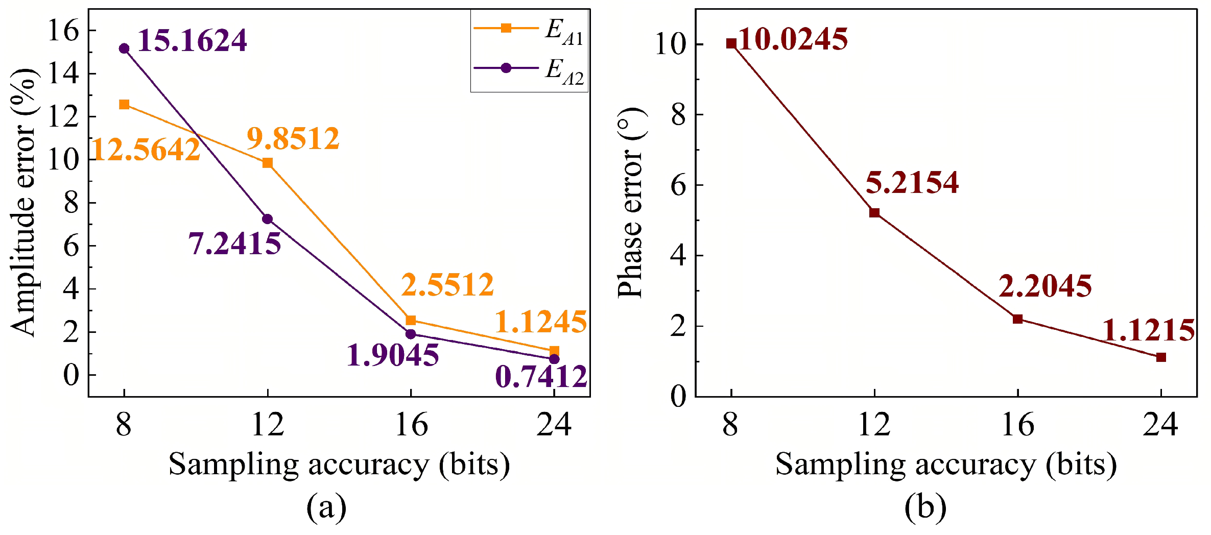
To further investigate the effect of sampling accuracy on the reconstruction of the crack amplitude–phase features at a constant sampling frequency, the signals S_b(t) in Figure 9 were selected for analysis. The reconstruction algorithm shown in Figure 3 was then applied. The amplitude and phase information were then extracted. Using the same method as that described in Section 3.2.1, the envelope peak points of different signals in Figure 9 were extracted. Equations (3) and (4) were then used to calculate the errors at sampling accuracies of 8, 12, 16, and 24 bits. The calculated amplitude error of the first envelope peak E_A1, the amplitude error of the second envelope peak E_A2, and the phase error of the crack detection signal $E_{\phi }$ are shown in Figure 10. The results are shown in Figure 10.

As shown in Figure 10, within the range of sampling accuracies tested in this study, when the sampling frequency is 64 kHz, the amplitude errors of the two envelope peaks and the phase error of the signal gradually decrease with increasing sampling accuracy. When the sampling accuracy reaches 16 and 24 bits, the decreasing trends of the amplitude and phase errors become less pronounced. At a sampling accuracy of 24 bits, both E_A1 and E_A2 reach their minimum values, which are approximately 1%. The phase error $E_{\phi }$ also reaches its minimum value of 1.1215°, indicating that the detection signal waveform is effectively reconstructed. Excessively high sampling accuracy leads to increased power consumption. Therefore, the sampling accuracy of the detection signal was set to 16 bits for the subsequent balanced field electromagnetic crack detection experiments.

3.2.3. Effects of Reference Accuracy on the Amplitude–Phase Feature Errors of Detection Signals

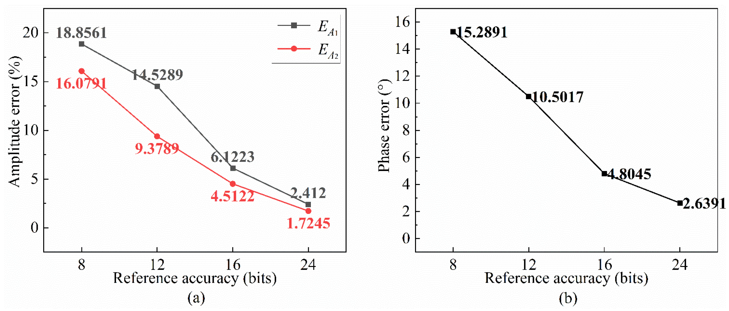
Within the range of sampling parameters tested in this study, Section 3.2.1 and Section 3.2.2 show that a sampling frequency of 64 kHz and a sampling accuracy of 16 bits provide satisfactory signal reconstruction. Under these conditions, the amplitude–phase features of the balanced field electromagnetic crack detection signal can be effectively reconstructed. Therefore, in this section, the sampling settings were kept unchanged. The reference accuracy H was set to 8, 12, 16, and 24 bits. The corresponding amplitude–phase feature errors of the crack detection signal were then analyzed to evaluate the effect of reference accuracy. Similarly, the envelope peaks were extracted and the errors were calculated using the methods described in Section 3.2.1. The amplitude error of the first envelope peak E_A1, the amplitude error of the second envelope peak E_A2, and the phase error of the crack detection signal $E_{\phi }$ under different reference accuracies are shown in Figure 11.

As shown in Figure 11, within the range of reference accuracies tested in this study, the amplitude errors of the two envelope peaks and the phase error of the signal decrease as the reference accuracy increases. When the reference accuracy reaches 16 bits, the reductions in amplitude and phase errors become less significant. The minimum errors are obtained at a reference accuracy of 24 bits. At a reference accuracy of 24 bits, EA1 and EA2 decrease to 2.412% and 1.7245%, respectively, while $E_{\phi }$ decreases to 2.6391°. These results indicate that the peak positions of the sampled detection signal are close to those of the simulated signal. Moreover, the amplitude–phase features of the crack detection signal are reconstructed with high fidelity. Compared with a reference accuracy of 24 bits, a reference accuracy of 16 bits resulted in higher amplitude and phase errors. Nevertheless, it was still sufficient to accurately reconstruct the amplitude–phase features of the crack detection signal. Additionally, excessively high reference accuracy increases hardware power consumption. Therefore, the reference accuracy was set to 16 bits in the subsequent balanced field electromagnetic crack detection experiments.

3.3. Influence of Sampling Parameters on the SNR of Detection Signals

To investigate the influence of sampling parameters on the SNR of the detection signals, different combinations of sampling frequency and sampling accuracy were configured for analysis with reference to Section 3.2. During crack detection, the defect-free portion of the detection signal corresponded to the time interval from 40 to 50 ms in Figure 5a. The signal within this interval was input into the algorithm shown in Figure 6 and extracted after simulated sampling. Taking a sampling frequency of 64 kHz as an example, the detection signals at defect-free positions obtained with sampling accuracies of 8, 12, 16, and 24 bits are shown in Figure 12.

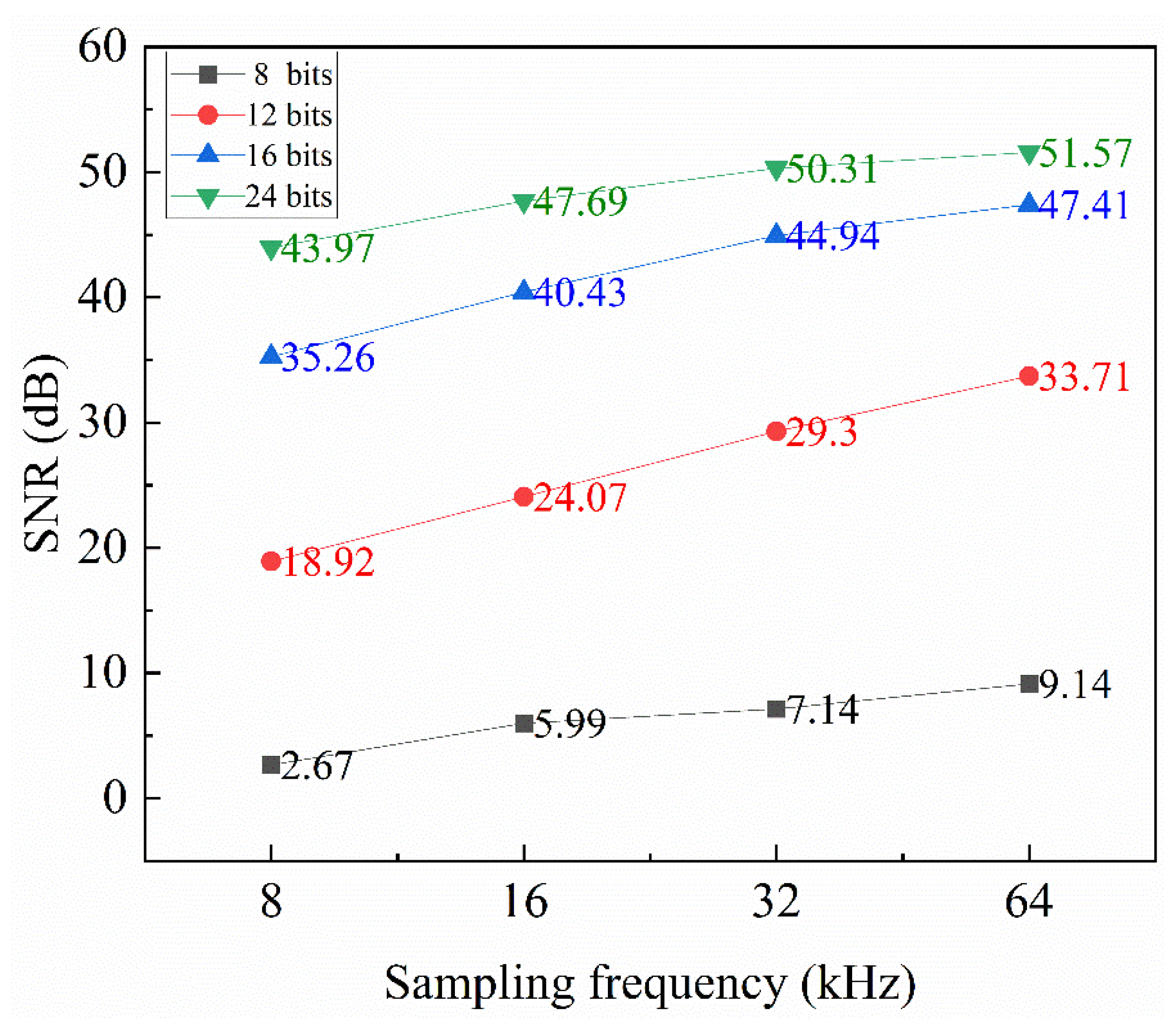
As shown in Figure 12, when the sampling accuracy is 8 bits, the detection signal exhibits an obvious step-like feature. When the sampling accuracy gradually increases to 16 bits or higher, the step-like behavior is barely observable, and the sensitivity to slight signal fluctuations is significantly enhanced. To analyze the effects of different sampling frequencies and sampling accuracies on the SNR of crack detection signals, the SNR defined in Equation (5) was used as the evaluation metric. Here, P_n represents the root-mean-square value of the signal derived from simulated sampling. This sampling was performed on the 40–50 ms detection signal in Figure 5a using the algorithm in Figure 6 under different combinations of sampling frequencies (8, 16, 32, and 64 kHz) and accuracies (8, 12, 16, and 24 bits). Under the parameter settings corresponding to P_n, the detection signal within the 40–50 ms interval in Figure 5a was processed using the algorithm in Figure 6. Simulated sampling was directly performed on this signal without adding Gaussian white noise or quantization noise, and P_s represents the root-mean-square value of the resulting signal. The calculated SNR results of the detection signals under different parameter combinations are shown in Figure 13.

$$SNR=20\lg \left({\displaystyle \frac{P_s}{P_n}}\right)$$

(5)

As shown in Figure 13, when the sampling accuracy is fixed, the SNR gradually increases with increasing sampling frequency. Similarly, when the sampling frequency is fixed, the SNR also increases as the sampling accuracy improves. The maximum detection SNR reaches 51.57 dB at a sampling frequency of 64 kHz and a sampling accuracy of 24 bits. When the sampling accuracy is 24 bits, increasing the sampling frequency from 32 to 64 kHz improves the SNR by 1.26 dB. When the sampling frequency is 64 kHz, increasing the sampling accuracy from 16 to 24 bits improves the SNR by 4.16 dB. However, as the sampling frequency and sampling accuracy increase, the improvement in SNR becomes limited, whereas the acquired data volume increases, imposing greater burdens on data storage and hardware power consumption. This study is based on a pipeline in-line inspection tool previously developed by our research group and deployed in engineering applications. During operation, the tool is powered by a limited-capacity onboard power supply and integrates multiple sensors, excitation and signal acquisition and processing units, positioning units, and data storage modules. Under long-duration multichannel operation, increasing the sampling parameters of a single channel can substantially increase power consumption and data storage demands. Therefore, the combination of a sampling frequency of 64 kHz with sampling accuracy and reference accuracy both set to 16 bits is more suitable for the practical applications of balanced field electromagnetic crack detection, and these parameters are adopted in the subsequent experiments.

4. Experiments and Results Analysis

To verify the influence of the sampling parameter settings described above on the variation trends in the amplitude–phase feature errors of crack detection signals, a signal feature sampling analysis system was developed, and an experimental platform for detection based on the BFET was established. All experiments in this study were conducted under dry conditions at room temperature and atmospheric pressure. The effects of hydrostatic pressure, the seawater environment, sealing reliability, and actual underwater motion on the detection performance have not yet been investigated.

4.1. Experimental Setup

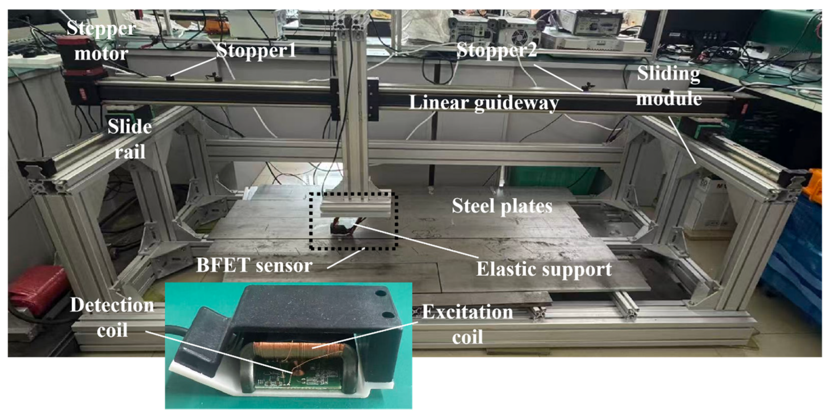
The overall detection platform for detection based on the BFET mainly consists of a stepper motor, stopper, linear guideway, slide rail, sliding module, elastic support, and BFET sensor. By controlling the stepper motor, high-precision position and speed control can be achieved, enabling more accurate crack defect detection using the balanced field electromagnetic sensor. The linear guideway converts the rotational motion of the stepper motor into the corresponding displacement or velocity, thereby driving the sensor to move. The sliding module works together with the stepper motor and linear guideway to complete translational motion and is used to switch between different steel plates under test. The elastic support ensures good contact between the sensor and the tested steel plate and applies appropriate pressure, thereby improving crack detection performance. The detection platform is shown in Figure 14.

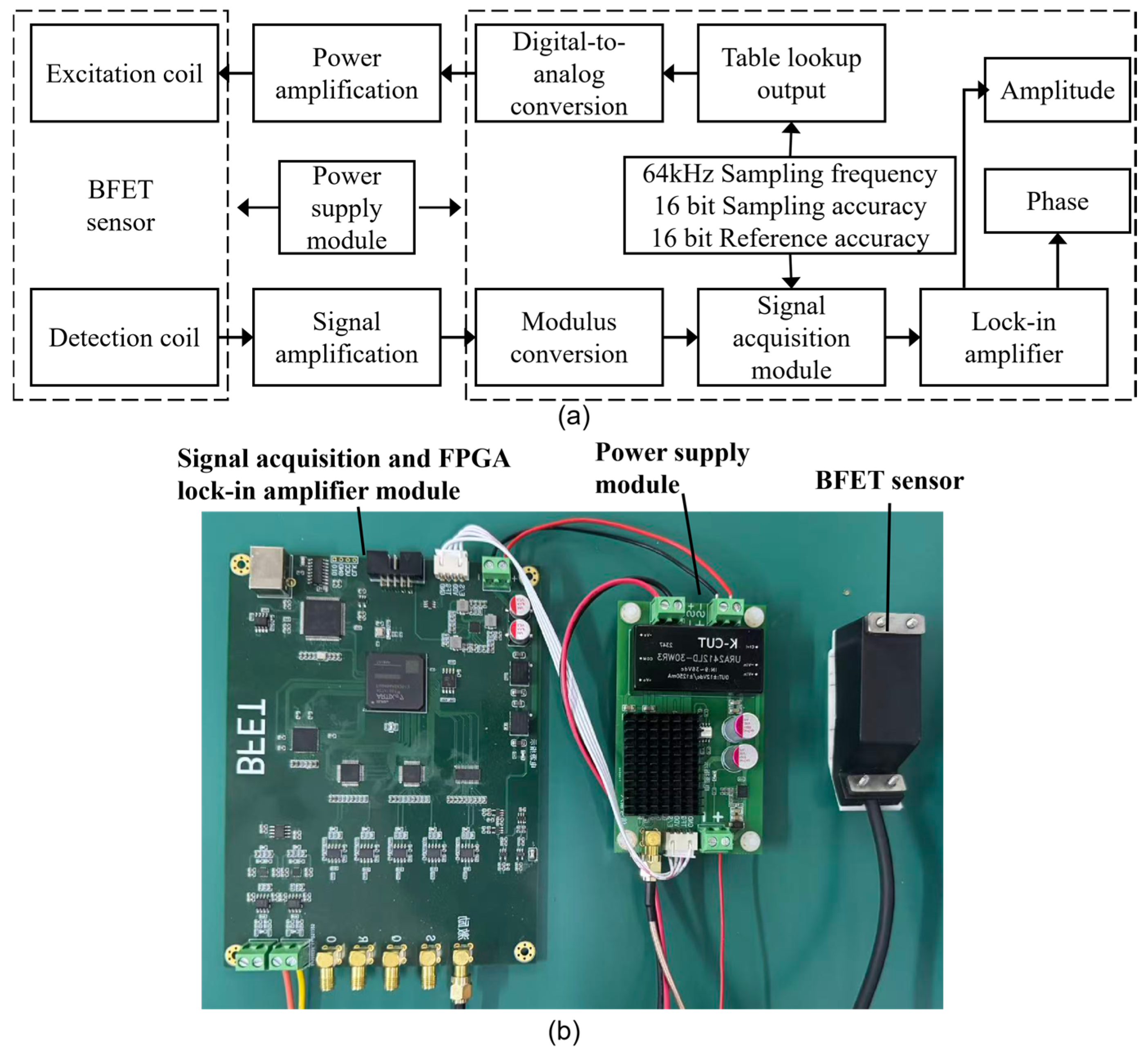
A sinusoidal alternating current with a frequency of 1 kHz was applied to the excitation coil. When the BFET sensor passed over a crack, distortion of the magnetic flux and induced current were generated on the steel plate surface. This distortion was then detected by the detection coil. The signal feature sampling analysis system, shown in Figure 15b, was used to acquire and process the detection signal simultaneously. Finally, the amplitude and phase of the crack detection signal were output. The working principle and physical prototype of the signal feature sampling analysis system are shown in Figure 15.

Figure 15b shows the signal feature sampling analysis system constructed according to the workflow shown in Figure 15a. The system consists of a signal acquisition and FPGA lock-in amplifier module, a power supply module, and a BFET sensor, as shown in Figure 15b. The sampling parameters were consistent with those analyzed in Section 3: the sampling frequency was set to 64 kHz, and both the sampling accuracy and reference accuracy were set to 16 bits.

4.2. Results Analysis and Discussion

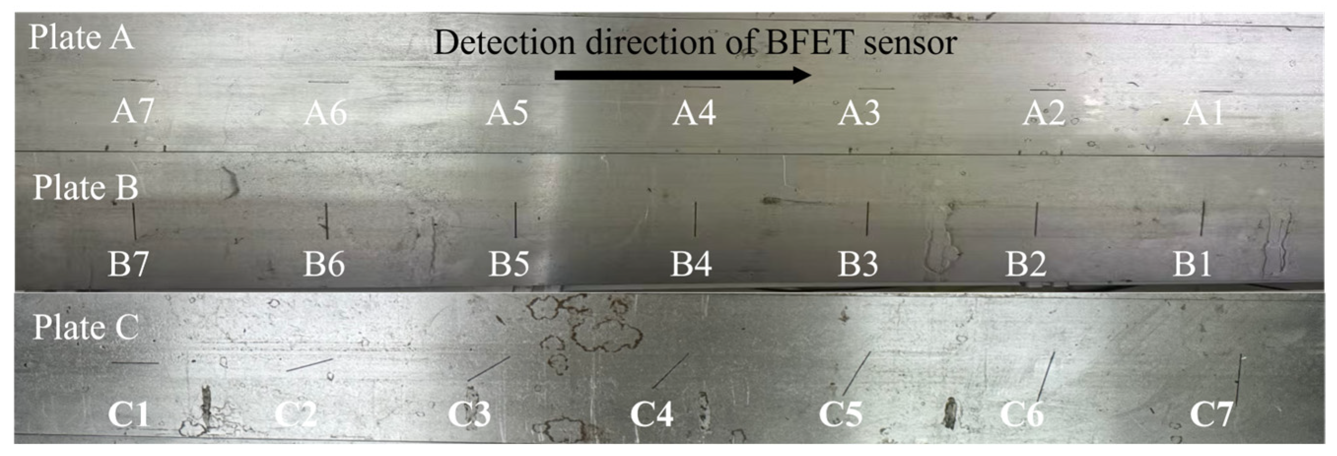
To verify the reconstruction accuracy of the developed signal feature sampling analysis system for the amplitude–phase features of crack detection signals and its influence on the SNR, experiments were conducted on Q235 steel plates with different defects fabricated by electrical discharge machining. The specific crack parameters are listed in

Table 2. Crack parameters.

Specimen Number	Crack Type	Parameters
plate A (A1–A7)	longitudinal crack	1–7 mm
plate B (B1–B7)	transverse crack	1–7 mm
plate C (C1–C7)	angled crack	0°, 15°, 30°, 45°, 60°, 75°, 90°

. Steel plates A, B, and C were all 1400 mm in length and 20 mm in width. The cracks were 40 mm in length and 0.3 mm in width for all specimens. The experimental specimens are shown in Figure 16.

Using the detection platform for detection based on the BFET and the signal feature sampling analysis system shown in Figure 14 and Figure 15, the experimental specimens with different crack parameters as shown in Figure 16 were inspected. The sliding module, together with the stepper motor and linear guide, enabled translational motion for the sensor to switch between different experimental specimens. The BFET sensor was set to scan the experimental specimens at a constant speed of 70 mm/s. At a sampling frequency of 64 kHz, the spatial interval between two adjacent original sampling points was approximately 1.09 μm. Because the excitation frequency was 1 kHz, each excitation cycle contained 64 sampling points, during which the sensor traveled approximately 0.07 mm. The signal feature sampling analysis system was used to output the amplitude and phase of the crack detection signals. Representative signals obtained from a single scan are shown in Figure 17.

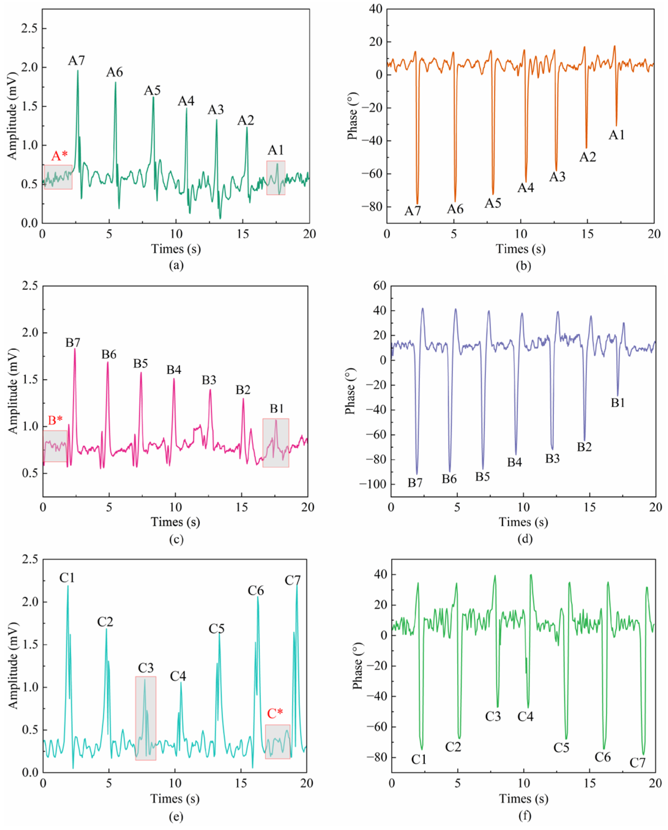
As shown in Figure 17, distinct amplitude and phase features are observed for transverse and longitudinal cracks with different depths, as well as for angled cracks. These results indicate that the developed signal feature sampling analysis system can effectively detect cracks. For both longitudinal and transverse cracks, the amplitude and phase signals gradually increase with increasing crack depth. For angled cracks, the amplitude and phase signals first decrease and then increase. This trend is consistent with previous studies on the BFET [12]. In Figure 17, A1, B1, and C3 denote the signals with the minimum amplitudes among the longitudinal, transverse, and angled crack signals, respectively. A*, B*, and C* represent the signals acquired at defect-free locations in the longitudinal, transverse, and angled crack detection data, respectively, and are used for the subsequent calculation of the signal-to-noise ratio.

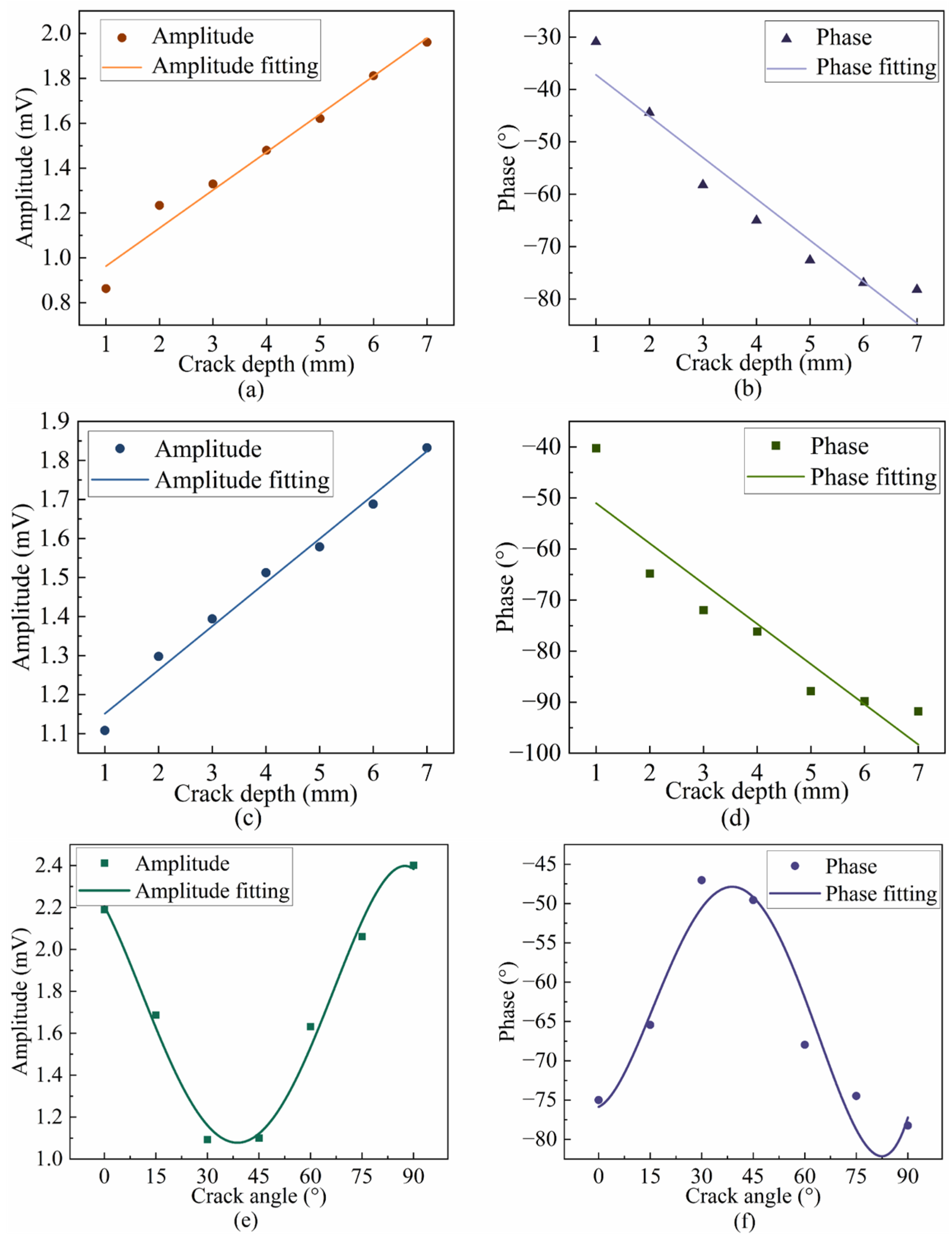
To further verify the effectiveness of a sampling frequency of 64 kHz and 16-bit sampling accuracy and reference accuracy in reconstructing the amplitude and phase features of cracks, the peak amplitudes and phase extrema of the crack detection signals were extracted. The extracted results from Figure 17a,c,e for amplitude, and Figure 17b,d,f for phase, were then fitted. The fitting results are shown in Figure 18.

As shown in Figure 18, with increasing crack depth, the absolute values of the amplitude and phase for both transverse and longitudinal cracks show a monotonic increasing trend. When the crack angle is within the range of 0–30°, the absolute values of the amplitude and phase gradually decrease with increasing crack angle. When the crack angle is within the range of 30–90°, the absolute values of the amplitude and phase gradually increase with increasing crack angle. This variation trend is consistent with a previous study by our research group [18]. These results indicate that the developed signal feature sampling analysis system, using the combination of 16-bit sampling accuracy, 16-bit reference accuracy, and a sampling frequency of 64 kHz, provides good reconstruction capability for the amplitude and phase features of cracks with different depths and angles.

To further evaluate the SNR of the detection signals obtained using the developed signal feature sampling analysis system, the minimum crack detection signal amplitudes, A1, B1, and C3, were extracted from Figure 17a, Figure 17c and Figure 17e, respectively, and the SNR was calculated using Equation (5). Here, the defect-free regions, denoted as A*, B*, and C*, in the detection signals shown in Figure 17 were selected to calculate the root-mean-square value P_n. The root-mean-square values P_s correspond to those of the crack detection signals A1, B1, and C3, respectively, under the same parameter settings. Under identical excitation, lift-off, scanning speed, and data acquisition conditions, five independent scans were performed on steel plates A, B, and C. Signals acquired at the same locations were extracted to calculate the signal-to-noise ratio. The mean signal-to-noise ratios of the crack detection signals obtained using different sampling parameters are presented in

Table 3. Mean SNRs of crack detection signals for different crack parameters.

Crack Type	1st (dB)	2nd (dB)	3rd (dB)	4th (dB)	5th (dB)	Mean SNR (dB)	Standard Deviation
longitudinal crack	38.20	36.79	35.82	38.37	36.92	37.22	1.06
transverse crack	34.80	32.14	34.90	35.50	35.71	34.61	1.43
angled crack	33.97	30.02	31.01	30.13	33.57	31.74	1.93

.

As shown in Table 3, cracks with different parameters result in different amplitudes of effective crack detection signals, leading to variations in the SNR. The SNRs of the crack detection signals for different crack parameters are all higher than 31 dB, with only a small variation range. The simulation assumed ideal conditions for the sensor, analog front end, and data acquisition process. In contrast, the experimental signals were additionally affected by sensor imbalance, analog-front-end noise, environmental electromagnetic interference, mechanical vibration, lift-off variation, and component nonidealities. Consequently, the experimental signal-to-noise ratios were lower than those predicted by the simulation. These results indicate that the signal feature sampling analysis system using the combination of 16-bit sampling accuracy, 16-bit reference accuracy, and a sampling frequency of 64 kHz provides relatively stable detection capability for cracks with different parameters while achieving a high SNR.

It should be noted that the experiments in this study primarily investigate the effects of the sampling parameters and reference accuracy on the reconstruction of the amplitude–phase features and the signal-to-noise ratio of balanced field electromagnetic crack detection signals, while also evaluating the implementation performance of the selected parameter configuration in the current detection system. Because the existing dataset does not adequately cover variations in crack type, depth, length, width, and orientation, it is insufficient for the development and independent validation of crack classification and sizing models. Future work will establish a larger annotated dataset covering a broader range of crack types and geometric parameters and will jointly analyze multiple features, including amplitude, phase, peak characteristics, spatial distribution, and waveform morphology, to investigate crack-type identification and quantitative crack sizing.

5. Conclusions

This study proposes a sampling-optimized high-SNR balanced field electromagnetic method for subsea pipeline crack detection to address the limited reconstruction accuracy of amplitude–phase features and the low signal-to-noise ratio caused by sampling parameters in complex subsea oil and gas pipeline inspection environments. A finite-element model of the BFET sensor was established, and the simulated detection signal obtained from this model was used as the theoretical signal to investigate the effects of sampling parameters. A signal feature sampling analysis algorithm was then developed. The effects of sampling frequency, sampling accuracy, and reference accuracy on the reconstruction accuracy of the amplitude–phase features of crack detection signals and on the SNR of detection signals were systematically analyzed. The main conclusions are as follows:

• Sampling frequency, sampling accuracy, and reference accuracy are important factors affecting the reconstruction accuracy of the amplitude–phase features of the BFET crack detection signals. An insufficient sampling frequency may lead to the loss of envelope peaks and waveform details in crack detection signals. Insufficient sampling accuracy reduces the resolution of crack detection signals and readily introduces step-like distortion. Insufficient reference accuracy reduces the resolution of the reference signal during digital lock-in demodulation. As a result, the accuracy of the in-phase and quadrature components is degraded, leading to poorer reconstruction of the amplitude and phase features in crack detection signals.
• Within the ranges of sampling parameters and reference accuracies investigated in this study, increasing the sampling frequency, sampling accuracy, and reference accuracy is beneficial for reducing errors in the amplitude–phase features of crack detection signals and improving their reconstruction capability. Considering the reconstruction performance of the amplitude and phase features, as well as the constraints of data volume and hardware power consumption, a sampling frequency of 64 kHz was selected. Both the sampling accuracy and the reference accuracy were set to 16 bits. This configuration provides a favorable overall trade-off and is suitable for practical applications of BFET crack detection in subsea pipelines.
• Sampling parameters are also among the key factors affecting the SNR of the BFET detection signals. As the sampling frequency increases, more sampling points are acquired per unit time, enabling the envelope variations and peak values of crack detection signals to be more faithfully preserved. This increases the root-mean-square value of the crack detection signal. Consequently, the signal-to-noise ratio is improved. As the sampling accuracy increases, both the quantization interval and the quantization error decrease. This reduces the RMS value of the noise and further improves the SNR. The sampling-optimized high-SNR balanced field electromagnetic method for subsea pipeline crack detection proposed in this study provides a useful reference for signal acquisition, amplitude–phase feature reconstruction, and SNR enhancement in other electromagnetic nondestructive testing methods.

References

1. Qu, F.; Chen, S.T.; Zhang, M.Y.; Zhang, K.; Gong, Y.J. Design and performance study of a magnetic flux leakage pig for subsea pipeline defect detection. J. Mar. Sci. Eng. 2025, 13, 1462. [Google Scholar] [CrossRef]
2. Zhu, H.; Chen, J.W.; Lin, Y.; Guo, J.; Gao, X.; Chen, Y.J.; Ge, Y.Q.; Wang, W. In-line inspection (ILI) techniques for subsea pipelines: State-of-the-art. J. Mar. Sci. Eng. 2024, 12, 417. [Google Scholar] [CrossRef]
3. Liu, B.; Ding, L.Y.; He, L.Y.; Yang, L.J.; Zhang, X.B.; Tian, Y. Residual generative adversarial network-driven data enhancement for magnetic flux leakage-based defect recognition in oil and gas pipelines. Eng. Appl. Artif. Intell. 2025, 162, 112720. [Google Scholar] [CrossRef]
4. Wu, Q.; Dong, K.; Qin, X.P.; Hu, Z.Q.; Xiong, X.C. Magnetic particle inspection: Status, advances, and challenges—Demands for automatic non-destructive testing. Ndt E Int. 2024, 143, 103030. [Google Scholar] [CrossRef]
5. Huang, S.L.; Peng, L.S.; Sun, H.Y.; Li, S.S. Deep learning for magnetic flux leakage detection and evaluation of oil & gas pipelines: A review. Energies 2023, 16, 1372. [Google Scholar] [CrossRef]
6. Lyu, F.; Zhou, X.Y.; Ding, Z.; Qiao, X.L.; Song, D. Application research of ultrasonic-guided wave technology in pipeline corrosion defect detection: A review. Coatings 2024, 14, 358. [Google Scholar] [CrossRef]
7. Parlak, B.O.; Yavasoglu, H.A. A comprehensive analysis of in-line inspection tools and technologies for steel oil and gas pipelines. Sustainability 2023, 15, 2783. [Google Scholar] [CrossRef]
8. Hu, Y.H.; Lu, L.L.; Zhan, S.F. Simulation and reliability evaluation of automated ultrasonic testing technology in semi-automatic welding of oil and gas pipelines. Int. J. Adv. Manuf. Technol. 2023, 124, 4131–4141. [Google Scholar] [CrossRef]
9. Jin, X.J.; Yang, L.J. Research on eddy current-based detection method for pipeline hard spots. Measurement 2026, 257, 118952. [Google Scholar] [CrossRef]
10. Gao, Z.H.; Zhang, H.G. Pipeline external defect detection based on magnetically focused eddy current testing system. Appl. Sci. 2025, 15, 11012. [Google Scholar] [CrossRef]
11. Liang, X.B.; Xu, C.J.; Zhang, X.; Jiang, W.M. A review of eddy current in-line inspection technology for oil and gas pipelines. Processes 2026, 14, 247. [Google Scholar] [CrossRef]
12. Zheng, W.X.; Li, J.Y.; Pan, Z.R.; Yang, L.J.; He, L.Y.; Liu, B. Balanced-field electromagnetic detection method for pipeline cracks with a high-frequency stability signal source. IEEE Trans. Instrum. Meas. 2025, 74, 1–10. [Google Scholar] [CrossRef]
13. Zheng, W.X.; Li, J.Y. Multi-channel frequency difference noise analysis and cancellation method for the balanced field electromagnetic pipeline inspection gauge. Rev. Sci. Instrum. 2023, 94, 074702. [Google Scholar] [CrossRef] [PubMed]
14. Zhang, Z.F.; Huang, J.; Yu, Y.L.; Qin, R.; Wang, J.; Zhang, S.; Su, Y.; Wen, G.R.; Cheng, W.; Chen, X.F. Microleakage acoustic emission monitoring of pipeline weld cracks under complex noise interference: A feasible framework. J. Sound Vib. 2025, 604, 118980. [Google Scholar] [CrossRef]
15. Li, W.; Wang, Z.R.; Yin, X.K.; Yuan, X.A.; Yang, H.M.; Shao, X.Y. Differential electromagnetic acoustic probes for quantitative detection of pipeline cracks. IEEE Sens. J. 2023, 23, 9820–9831. [Google Scholar] [CrossRef]
16. Li, J.L.; Jiang, J.S.; Fan, X.H.; Wang, H.Q.; Song, L.Y.; Liu, W.B.; Yang, J.F.; Chen, L.C. A new method for weak fault feature extraction based on improved MED. Shock. Vib. 2018, 2018, 9432394. [Google Scholar] [CrossRef]
17. Bai, J.S.; Yao, J.J.; Yang, Z.L.; Guo, Y.R.; Wang, L.M. Transient electromagnetic weak signal extraction method based on multi-scale combined difference product morphological filtering. IEEE Access 2022, 10, 22140–22149. [Google Scholar] [CrossRef]
18. Zheng, W.X.; Li, J.Y.; Pan, Z.R.; Li, Y.J.; Liu, B. Balanced field electromagnetic pipeline crack detection method with multiple-correlation demodulation. IEEE Trans. Instrum. Meas. 2026, 75, 1–10. [Google Scholar] [CrossRef]
19. Huang, S.H.; Hong, M.C.; Lin, G.; Tang, B.; Shen, S.B. A discrete fourier transform-based signal processing method for an eddy current detection sensor. Sensors 2025, 25, 2686. [Google Scholar] [CrossRef] [PubMed]
20. Xia, Z.T.; Jia, J. Non-destructive eddy current testing system based on discrete wavelet transform. Electronics 2025, 14, 3239. [Google Scholar] [CrossRef]
21. Zhang, C.; Li, J.; Qin, L.; Zhang, X.; Zhang, D.B.; Feng, K.Q.; Hu, C.J.; Li, P.B. Signal-to-noise ratio enhancement method for weak signals: A joint optimization strategy based on intelligent optimization iterative algorithm. Electronics 2025, 14, 4914. [Google Scholar] [CrossRef]
22. Zheng, W.X.; Li, J.Y.; Xiao, Y.X. Processing methods of the pipeline crack detection signal by a balanced field electromagnetic technique based on phase characteristics. Rev. Sci. Instrum. 2023, 94, 044706. [Google Scholar] [CrossRef] [PubMed]
Figure 1. Schematic illustration of subsea pipeline inspection.
Jmse 14 01416 g001
Figure 2. Schematic illustration of the BFET sensor.
Jmse 14 01416 g002
Figure 3. Principle diagram of the digital lock-in amplification process for the BFET detection signals.
Jmse 14 01416 g003
Figure 4. Finite-element model of the BFET sensor.
Jmse 14 01416 g004
Figure 5. Simulated signals. (a) Original crack detection signal. (b) Amplitude of the original crack detection signal. (c) Phase of the original crack detection signal.
Jmse 14 01416 g005
Figure 6. Workflow of the signal feature sampling analysis algorithm.
Jmse 14 01416 g006
Figure 7. Crack detection signals sampled at different sampling frequencies with a sampling accuracy of 16 bits.
Jmse 14 01416 g007
Figure 8. Amplitude–phase errors at different sampling frequencies with a sampling accuracy of 16 bits. (a) Amplitude errors at different sampling frequencies with a sampling accuracy of 16 bits. (b) Phase errors at different sampling frequencies with a sampling accuracy of 16 bits.
Jmse 14 01416 g008
Figure 9. Crack detection signals sampled at different sampling accuracies with a sampling frequency of 64 kHz.
Jmse 14 01416 g009
Figure 10. Amplitude–phase errors at different sampling accuracies with a sampling frequency of 64 kHz. (a) Amplitude errors at different sampling accuracies. (b) Phase errors at different sampling accuracies.
Jmse 14 01416 g010
Figure 11. Amplitude–phase errors under different reference accuracies. (a) Amplitude errors under different reference accuracies. (b) Phase errors under different reference accuracies.
Jmse 14 01416 g011
Figure 12. Detection signals at defect-free positions with different sampling accuracies.
Jmse 14 01416 g012
Figure 13. SNR calculation results.
Jmse 14 01416 g013
Figure 14. Detection platform of BFET.
Jmse 14 01416 g014
Figure 15. Working principle and prototype of the signal feature sampling analysis system. (a) Working principle. (b) Physical prototype.
Jmse 14 01416 g015
Figure 16. Specimens used in the experiments.
Jmse 14 01416 g016
Figure 17. Amplitude–phase features of crack detection signals for cracks with different parameters. (a) Amplitude of the longitudinal crack detection signal. (b) Phase of the longitudinal crack detection signal. (c) Amplitude of the transverse crack detection signal. (d) Phase of the transverse crack detection signal. (e) Amplitude of the angled crack detection signal. (f) Phase of the angled crack detection signal.
Jmse 14 01416 g017
Figure 18. Fitting results of the amplitude–phase features of crack detection signals for different crack parameters. (a) Amplitude fitting for longitudinal cracks. (b) Phase fitting for longitudinal cracks. (c) Amplitude fitting for transverse cracks. (d) Phase fitting for transverse cracks. (e) Amplitude fitting for angled cracks. (f) Phase fitting for angled cracks.
Jmse 14 01416 g018