Study on the Shallow Water Effect Characteristics of Tankers in Pile-Founded Column Single Point Mooring Systems

Abstract

To ensure the safety and stability of single point mooring (SPM) systems operating in shallow waters, this paper investigates the influences of shallow-water effects on mooring systems under different water depth-to-draft ratios. For the pile-founded column single point mooring system in shallow sea areas, based on the numerical calculation method verified by model tests, frequency domain and time domain calculations are carried out to study the specific impact of shallow water effects on the hydrodynamic parameters of the hull, and the critical water depth-to-draft ratios applicable to the two second-order wave load calculation methods (Newman approximation and Pinkster approximation) are analyzed. At the same time, the specific impact of shallow water effects on the dynamic response of the mooring system under three different hull loading conditions at the same and different water depth-to-draft ratios is studied, and the critical water depth conditions for bottom contact in each loading condition are summarized. The results show that the shallow water effect has a significant impact on the hydrodynamic parameters such as RAO of the hull response, especially in the low-frequency response region. There are obvious differences between the Newman approximation and the Pinkster approximation methods. In shallow water conditions, the Pinkster approximation method has a more accurate calculation effect, and when the water depth-to-draft ratio reaches a certain critical value, the calculation results of the two approximation methods are basically consistent. For the same and different water depth-to-draft ratio conditions, the amplitude of the hull motion in the full-load draft state is greater than the other two loading conditions, but the response results of the cable tension are opposite. The research results reveal the specific influences of shallow-water effects on pile-supported single-point mooring (SPM) systems, which can provide references for the safety and stability design of mooring systems and bear great engineering significance for advancing the deployment of single-point mooring systems in shallow water regions.

1. Introduction

With the increasing demand for the development of marginal offshore oil fields, offshore oil and gas facilities are gradually extending toward shallow and even ultra-shallow water regions. Single Point Mooring (SPM) systems have been widely adopted in offshore oil production due to their unique weathervaning capability. Under the combined effects of wind, waves, and current, an SPM-based floating production storage and offloading (FPSO) unit can automatically adjust its heading and rotate toward a direction with relatively lower environmental loads, thereby reducing the overall environmental forces acting on the system.

Previous studies have shown that the weathervaning behavior of FPSO units is governed by the combined effects of wind-induced yaw moment, wave drift moment, current-induced moment, and mooring restoring moment. Essentially, this process represents a dynamic equilibrium among different environmental moments while the vessel rotates around the single-point mooring center. Khor and Barltrop [1] investigated the extreme responses of a floating and weathervaning platform under different combinations of wind, wave, and current directions, demonstrating that the misalignment between environmental loads can significantly affect the vessel responses and mooring loads. In recent years, the weathervaning behavior of FPSOs, including numerical simulations, model experiments, and dynamic response analyses, has remained an active research topic in offshore engineering.

However, existing SPM systems are mainly deployed in medium- and deep-water areas, with typical operating water depths exceeding 20 m. For marginal oil fields located in shallow or ultra-shallow waters (less than 20 m), conventional catenary-based SPM systems face considerable challenges due to limitations associated with water depth, foundation arrangement, and available mooring space. Therefore, the development of efficient and reliable SPM systems suitable for shallow-water environments remains a technical challenge.

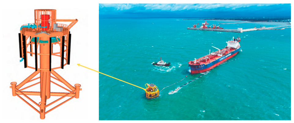
To address this issue, China National Offshore Oil Corporation (CNOOC) has recently proposed a pile-supported column-type single point mooring system (Figure 1) for offshore oil exploitation in shallow-water regions. The upper structure consists of an independent column-type turret, while the subsea foundation adopts a 20 m × 20 m four-skirt-pile configuration. The upper rotating structure is connected to the subsea foundation through a main bearing, and crude oil transportation is achieved through a 610 mm diameter oil swivel connected to the pipeline system. This configuration enables shuttle tankers to continuously perform crude oil offloading operations while rotating around the single point under the action of the weathervaning effect [2].

Under complex ocean environmental conditions, floating structures are subjected not only to first-order wave loads but also to second-order wave forces induced by arbitrary bichromatic waves. Second-order wave forces can generally be classified into three categories: mean drift forces, difference-frequency forces, and sum-frequency forces. For oil tankers, wind loads, current loads, first-order wave forces, as well as the sum-frequency and mean drift components of second-order forces, are generally insensitive to variations in water depth. In contrast, the difference-frequency force is highly sensitive to water depth changes. In shallow-water environments, floating bodies are prone to significant low-frequency motion responses, which is the fundamental mechanism underlying shallow-water effects.

Second-order wave forces are the primary excitation source inducing low-frequency motions in single-point mooring systems. The theoretical foundation can be traced back to the approximation method for difference-frequency forces proposed by Newman [3]. By simplifying the quadratic transfer function (QTF) of second-order forces, this method provides an effective engineering approach for calculating low-frequency drift forces, although its applicability under complex sea states remains somewhat limited. Pinkster and Oortmerssen [4] proposed the near-field method, in which direct pressure integration over the body surface is performed to obtain six-degree-of-freedom second-order wave loads in both horizontal and vertical planes. However, compared with the far-field method, the near-field approach is relatively complex and computationally time-consuming. In addition, the mesh quality of the wetted surface has a significant influence on the convergence of the numerical results. In recent years, many researchers (Drake [5]; Chang [6]; Carmo and Simos [7]; Li et al. [8]) have adopted various approximate methods to address second-order low-frequency wave force problems.

Based on the Boussinesq equations, Park [9] conducted numerical investigations on nonlinear shallow-water wave processes involving varying seabed topography, with particular emphasis on the dynamic response of moored floating vessels under wave transformation effects. The results were compared with those obtained under the assumption of uniform water depth. The study demonstrated that seabed topography has a significant influence on shallow-water wave propagation characteristics and vessel motion responses and therefore cannot be neglected. Fonseca and Pessoa [10] employed a combined approach of model experiments and numerical simulations to systematically investigate the influence of water depth variation on first- and second-order wave forces acting on fixed floating bodies. Their results indicated that the effect of second-order wave forces in shallow water is non-negligible, and that these forces increase significantly as water depth decreases. Through numerical analysis, Zhang [11] verified that the contribution of second-order low-frequency wave loads becomes increasingly pronounced with decreasing water depth, particularly in the pitch direction. Yang et al. [12] similarly pointed out that the inclusion of low-frequency wave forces is essential in both horizontal and vertical motion analyses. From this perspective, the near-field method demonstrates considerable practical value, as it can provide solutions for all six degrees of freedom. Huo et al. [13] investigated the yaw oscillation characteristics of single-point moored vessels in shallow water through a combination of experiments and numerical analyses. The results showed that shallow-water environments significantly increase both the occurrence probability and oscillation amplitude of fishtailing motions. The study further indicated that wave deformation, flow field variation, and increased mooring stiffness in shallow water collectively make the system more susceptible to instability, while the coupled effects of wind, current, and wave loads further amplify the unstable response.

Cai Yuanlang et al. [14] conducted experimental investigations on the low-frequency motion response of shallow-water soft-yoke single point mooring systems and revealed that the presence of low-frequency waves could increase the surge motion amplitude to approximately twice that of the conventional response. Xiao Longfei et al. [15] carried out numerical simulations and model experiments on ultra-shallow-water soft-yoke single point mooring systems, demonstrating that under shallow-water conditions, the effects of first-order low-frequency wave forces and shallow-water long waves on the mooring system must be fully considered.

Yu Xiaochuan et al. [16] employed numerical methods to investigate the motion responses and load transfer functions of FPSOs under different water depth conditions. The results indicated that when the wavelength-to-ship-length ratio (λ/L) is less than 1, the ship motion response tends to become milder as the water depth decreases. Based on potential flow numerical methods, Xiao Longfei [17] analyzed the variation characteristics of FPSO hydrodynamic coefficients under different water depths and loading conditions. The study revealed that with decreasing water-depth-to-draft ratio, both the added mass and damping coefficients increase significantly, while the motion responses in the vertical plane become more moderate. Liu Chengyi [18] adopted both the Newman approximation and the Pinkster approximation to investigate the mooring force characteristics of three FPSOs with different tonnages under varying water-depth-to-draft ratios, and identified the critical water-depth-to-draft ratios at which shallow-water effects must be considered for different vessel types and draft conditions. Xie Zhen [19] applied three-dimensional potential flow theory to conduct frequency-domain analyses of shallow-water soft-yoke single-point mooring systems, taking draft and water depth as variables to investigate the first- and second-order shallow-water response characteristics of FPSOs. Based on potential flow theory, Zhan Yanmin et al. [20] analyzed the variation laws of the natural periods and motion response amplitude operators (RAOs) of vessels under different water depths.

At present, research on shallow-water effects of single point mooring systems mainly focuses on calculation methods for low-frequency wave forces, while relatively few studies have systematically investigated the hydrodynamic characteristics of shallow-water single point mooring systems under combined wind, wave, and current conditions. In particular, the specific influence mechanisms of shallow-water effects on single point mooring systems have not yet been clearly clarified from the perspectives of vessel motion responses and mooring load characteristics. Therefore, based on an actual engineering project, this study investigates the shallow-water effect characteristics of a pile-supported single point mooring system designed for shallow-water applications. The main research contents are summarized as follows: (1) A numerical model was established using AQWA, and the accuracy of the numerical method was validated through comparison with model test results. (2) Frequency-domain analyses under different water depth conditions were carried out to investigate the variation characteristics of hydrodynamic parameters, including added mass, radiation damping, RAOs, and QTF matrices, with changing water depth. (3) Time-domain analyses of the pile-supported single point mooring system under combined wind, wave, and current conditions were performed to evaluate the applicability of the Newman approximation and Pinkster approximation under different water-depth-to-draft ratios. (4) The motion responses and extreme mooring line tension characteristics under three loading conditions were analyzed for both identical and varying water-depth-to-draft ratios, and the variation laws of the dynamic responses of the single point mooring system with loading condition and water-depth-to-draft ratio were investigated. (5) Based on the calculation results under different water-depth-to-draft ratios, statistical analyses of vessel grounding conditions under three loading conditions were conducted. The corresponding critical water-depth-to-draft ratios and water depths associated with vessel grounding were identified, and the maximum motion amplitudes of the vessel in both vertical and horizontal planes under different loading conditions and water-depth-to-draft ratios were analyzed.

2. Establishment and Verification of Numerical Calculation Models

2.1. Numerical Calculation Model

In this study, the hydrodynamic potential flow software AQWA (2020) was employed to numerically calculate the motion responses of the prototype vessel and the mooring line tensions. Within the framework of potential flow theory, the fluid motion in the computational domain is described by a time-dependent velocity potential function Φ(x, y, z, t) [21]. For incompressible and irrotational fluid flow, the governing equation can be simplified into the Laplace equation within the fluid domain:

$${\nabla }^2\Phi ={\displaystyle \frac{{\partial }^2\Phi }{\partial x^2}}+{\displaystyle \frac{{\partial }^2\Phi }{\partial y^2}}+{\displaystyle \frac{{\partial }^2\Phi }{\partial z^2}}=0$$

(1)

The velocity potential function is required to satisfy the boundary conditions on the body surface, seabed, and free surface [22]. According to the classical formulation, the total potential is decomposed into incident, diffraction, and radiation components [23]. Based on the solved potential field, hydrodynamic coefficients such as added mass, radiation damping, and wave excitation coefficients, as well as the response amplitude operators (RAOs), can be obtained.

When wind loads, wave loads, current loads, and mooring forces are taken into account, the six-degree-of-freedom motions of the platform in the time domain can be expressed as follows [24]:

$$(M+\Delta M)\ddot{X}+(B_{rad}+B_{vis})\dot{X}+(K_{stillwater}+K_{mooring})X=F_1+F_{2low}+F_{2high}+F_{\mathit{wind}}+F_{current}+F_{othres}$$

(2)

where $\ddot{X}$ represents the vessel acceleration, $\dot{X}$ represents the vessel velocity, and $X$ represents the vessel displacement. $M$ denotes the structural mass matrix of the platform, $\Delta M$ is the added mass matrix, $B_{rad}$ is the radiation damping matrix, $B_{vis}$ is the viscous damping matrix, $K_{stillwater}$ represents the hydrostatic restoring stiffness, and $K_{mooring}$ denotes the mooring stiffness matrix. $F_1$ is the first-order wave-frequency load, $F_{2low}$ is the second-order low-frequency load, $F_{2high}$ is the second-order high-frequency load, $F_{wind}$ represents the wind load, $F_{current}$ denotes the current load, and $F_{othres}$ represents other external loads.

The second-order difference-frequency wave force is a low-frequency, slow-drift force generated by the interaction between wave components with different frequencies in irregular waves. It may induce long-period and large-amplitude horizontal motions of floating bodies and can easily trigger resonance responses in mooring systems. The second-order difference-frequency wave force can be expressed as follows:

$$\begin{array}{l}{F}^{(2)}(t)={\displaystyle \sum _{i=1}^N{\displaystyle \sum _{j=1}^N\left\{P_{ij}^{-}\cos [-({\omega }_i-{\omega }_j)t-({\epsilon }_i-{\epsilon }_j)]\right\}}}\\ +{\displaystyle \sum _{i=1}^N{\displaystyle \sum _{j=1}^N\left\{Q_{ij}^{-}\sin [-({\omega }_i-{\omega }_j)t-({\epsilon }_i-{\epsilon }_j)]\right\}}}\end{array}$$

(3)

where $P_{ij}^{-}$ and $Q_{ij}^{-}$ represent the real and imaginary parts of the second-order wave force transfer function, respectively. These quantities are only related to wave frequency and are independent of wave amplitude. ${\omega }_i$ and ${\omega }_j$ denote the frequencies of the two incident waves, while ${\epsilon }_i$ and ${\epsilon }_j$ represent the corresponding random phase angles of the two incident wave components.

As a classical approach for calculating second-order difference-frequency wave forces, the Newman approximation was first proposed by Newman in 1967 and is mainly used to evaluate second-order difference-frequency wave forces acting on floating structures in the horizontal plane. In this method, the diagonal elements of the second-order difference-frequency wave load transfer function matrix are employed to approximate the off-diagonal elements. On the premise of maintaining reasonable accuracy for difference-frequency excitation calculations, this approach avoids the complicated computation process associated with second-order velocity potentials and significantly reduces the overall computational cost, thereby demonstrating considerable engineering practicality. The transfer function obtained using this method can be expressed as follows:

$$\begin{array}{l}{P}_{ij}^{-}=P_{ji}^{-}=0.5\left(P_{ii}^{-}+P_{jj}^{-}\right)\\ Q_{ij}^{-}=Q_{ji}^{-}=0\end{array}$$

(4)

It can be observed from the equation that when the maximum or minimum values appear near the diagonal region of the transfer function matrix, as is often the case under shallow-water conditions, relatively large approximation errors may occur, leading to a serious underestimation of the actual low-frequency wave forces.

The Pinkster approximation, proposed by Pinkster in 1980, is another important method for calculating second-order difference-frequency wave forces. This method enables the evaluation of the second-order transfer function matrix for all six degrees of freedom, and the corresponding formulation is given as follows. By performing direct pressure integration, the real and imaginary components of the second-order difference-frequency wave transfer function matrix are calculated, thereby obtaining the complete QTF matrix. In this method, the approximation mainly lies in the treatment of the second-order potential function.

$$\begin{array}{l}{P}_{ij}^{(\pm )}=-{\displaystyle {\oint }_{WL}\frac{1}{4}}\rho g{\zeta }_j{\zeta }_i\cos ({\epsilon }_i\pm {\epsilon }_j){\displaystyle \frac{\overrightarrow{N}}{\sqrt{n_1^2+n_2^2}}}dl\\ +{\displaystyle {\iint }_{S_0}\frac{1}{4}}\rho |\nabla {\varphi }_i|\cdot |\nabla {\varphi }_j|\overrightarrow{N}dS\\ +{\displaystyle {\iint }_{S_0}\frac{1}{2}}\rho \left(X_i\cdot \nabla {\displaystyle \frac{\partial {\mathsf{\Phi }}_j}{\partial t}}\right)\overrightarrow{N}dS\\ +{\displaystyle \frac{1}{2}}{M}_s{R}_i\cdot {\overrightarrow{X}}_{gi}+{\displaystyle {\iint }_{S_0}\frac{1}{2}}\rho {\displaystyle \frac{\partial {\mathsf{\Phi }}^{(2)}}{\partial t}}\overrightarrow{N}dS\end{array}$$

(5)

The above equation consists of five components. The first term represents the contribution of the relative wave elevation, the second term corresponds to the hydrodynamic pressure induced by the square of the first-order velocity, the third term describes the coupling effect between the first-order pressure gradient and first-order motions, the fourth term represents the rotational effect of the first-order external forces, and the fifth term corresponds to the contribution of the second-order velocity potential.

The Newman approximation simplifies the off-diagonal elements of the QTF matrix, resulting in wave energy being primarily concentrated around the wave-frequency region while weakening the low-frequency response. Consequently, under shallow-water conditions, this method tends to significantly underestimate second-order low-frequency wave forces and is therefore unsuitable for shallow-water environments. In contrast, the Pinkster method can accurately capture the low-frequency energy distribution. Under deep-water conditions, the results obtained from the two methods show relatively small differences and exhibit similar trends.

The numerical calculation model is shown in Figure 2.

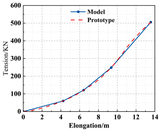
The principal parameters of the vessel are listed in

Table 1. Principal Parameters of the Vessel.

Principal Parameters	Ballast Condition	Intermediate Loading Condition	Fully Loaded Condition
Length overall/m	220.4	220.4	220.4
Length between perpendiculars/m	224.9	224.9	224.9
Breadth/m	35	35	35
Depth/m	18	18	18
Mean draft/m	6.91	9.936	11.166
Displacement/kg	41,177,800	62,360,000	71,448,100
Longitudinal center of gravity/m	113.643	116.236	113.431
Vertical center of gravity/m	7.972	9.889	10.780
Radius of gyration in roll/m	13.233	10.704	8.778
Radius of gyration in pitch/m	57.847	57.577	44.247
Radius of gyration in yaw/m	60.303	58.092	44.727
Metacentric height/m	10.450	5.113	3.810

. The mooring line stiffness characteristics are shown in Figure 2, and the corresponding material properties are listed in

Table 2. Mooring Line Material Properties.

Parameter	Length	Diameter	Linear Weight	Breaking Strength
	70 m	144 mm	12.8 kg/m	650 t

.

Since the numerical calculations were carried out using a potential flow solver, the effects of fluid viscosity were neglected. Therefore, a free decay test under calm-water conditions was conducted in this study. By introducing additional damping corrections into the numerical model, free decay simulations under the same conditions as the experiments were performed. The damping correction values applied to the vessel model were determined through comparison between the numerical and experimental decay curves. Different damping characterization approaches are adopted for various motion modes in this paper. For roll, pitch and heave, their damping characteristics are dominated by linear viscous damping, while the quadratic nonlinear damping component is also taken into account. The linear and quadratic damping coefficients are simultaneously identified via fitting free decay curves.

Due to the existence of quadratic damping, the equivalent damping coefficient of each mode varies to a certain extent with motion amplitude. In terms of roll and pitch motions, the nonlinear damping effect becomes prominent under large motion amplitudes; adopting merely linear damping will underestimate energy dissipation caused by damping. At small amplitudes, the linear damping term dominates, and the contribution of quadratic damping is relatively limited. For sway motion, the characterization accuracy of equivalent linear damping declines in the small-amplitude decay stage, leading to visible discrepancies between numerical and experimental curves. Considering multiple error sources, including wave reflection in basin tests, the curve deviation in the small-amplitude region exerts a negligible overall influence on the corrected damping results.

Viscous damping correction is implemented in ANSYS AQWA (2020) by introducing an Additional Damping Matrix. After completing frequency-domain hydrodynamic coefficient calculations in AQWA-LINE, the viscous damping coefficients corresponding to each degree of freedom are imported in the form of a damping matrix. The diagonal elements of the matrix separately represent the damping coefficients of the six degrees of freedom, namely surge, sway, heave, roll, pitch and yaw. Since coupling damping terms between different DOFs have minor impacts, all off-diagonal coupling items are set to zero.

2.2. Model Test

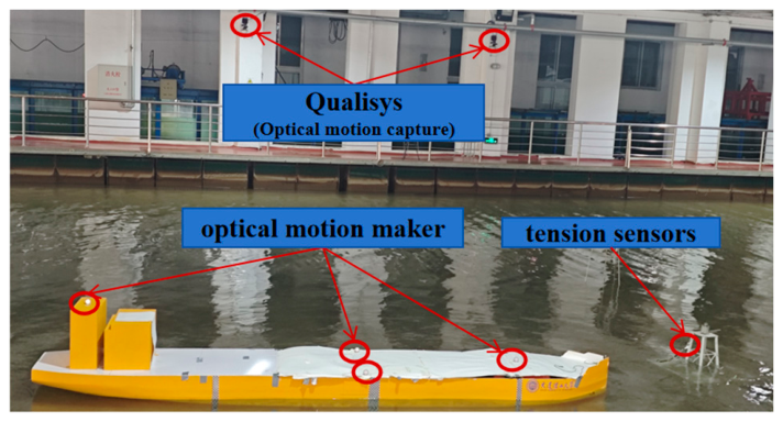
The experiments were conducted in the offshore engineering basin of the State Key Laboratory of Coastal and Offshore Engineering at Dalian University of Technology. The primary measurement instruments used in the tests included wave gauges, current meters, wind speed sensors, load cells, and a motion capture system. The application of the experimental instruments is illustrated in Figure 3. The mooring line tensions were measured using load cells manufactured by Yangzhou Kedong, with a measurement accuracy of 0.05%. Current velocity measurements were obtained using the Nortek Vectrino three-dimensional point current meter. Vessel motion trajectories were recorded using the Qualisys three-dimensional motion capture and analysis system developed in Germany, which provides a measurement accuracy better than 0.3 mm and is capable of accurately capturing the trajectories of high-speed moving objects.

Figure 3. Layout of Experimental Instruments.

Figure 3. Layout of Experimental Instruments.

The vessel model and jacket structure model were manufactured based on Froude similarity, with a model scale ratio of 1:50. The principal parameters of the vessel model can be derived according to Table 1. For the mooring lines, multiple springs and inextensible ropes were employed to ensure both geometric similarity and elastic similarity. The simulated stiffness characteristics of the mooring lines are shown in Figure 4.

Figure 4. Comparison of stiffness curves between the mooring line model and the actual mooring line.

Figure 4. Comparison of stiffness curves between the mooring line model and the actual mooring line.

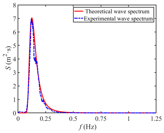
The detailed parameters of the experimental conditions (prototype scale) used for validating the numerical calculations in this study are listed in

Table 3. Environmental Parameters.

Condition	Significant Wave Height/m	Spectral Peak Period/s	Current Velocity/m/s	Wind Velocity/m/s	Direction/°
A-1	2	10	0.9	15	180
A-2	3	8	0.9	15	180
A-3	3	10	0.9	15	180

. Here, HS, TP, and γ represent the significant wave height, spectral peak period, and peak enhancement factor, respectively. The irregular waves were simulated using the JONSWAP spectrum, as expressed in Equations (6) and (7), with the peak enhancement factor γ taken as 1:

$$S(f)=\beta H_S^2{T}_P^{(-4)}{f}^{(-5)}exp[-1.25{(f/f_p)}^{(-4)}]{\gamma }^{exp[-{(f-f_p)}^2/2{\sigma }^2{f_p}^2]}$$

(6)

$$\beta ={\displaystyle \frac{5}{16}}{(1.15+0.1688\gamma -{\displaystyle \frac{0.925}{(1.909+\gamma )}})}^{(-1)}(1.094-0.1915ln\gamma )$$

(7)

The comparison between the theoretical spectrum and the experimental spectrum is shown in Figure 5. It can be observed that the two spectra exhibit good agreement.

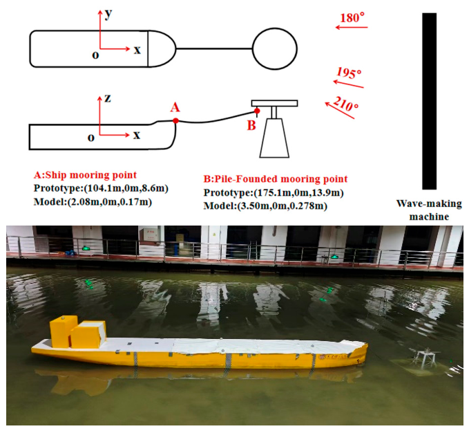
Taking the vessel center of gravity as the coordinate origin, the coordinates of the mooring points on the vessel and those on the pile-supported jacket structure at prototype scale are shown in Figure 6. After arranging the model according to the specified positions, the current generation system was activated, and the current velocity was monitored in real time. Once the flow velocity became stable, the wind generation system was initiated and maintained for a period to ensure stable conditions. Subsequently, the wave maker was started to generate the required irregular waves. Data acquisition began one minute after the irregular waves reached the model location. The sampling duration was 26 min, corresponding to approximately 3 h at prototype scale, and each test condition was repeated three times.

2.3. Validation of Numerical Model Against Model Test Results

The experimental results under the combined collinear action of wind, wave, and current at 180° were converted to the corresponding prototype-scale values based on Froude similarity and subsequently compared with the numerical simulation results. The corresponding environmental parameters are listed in Table 3.

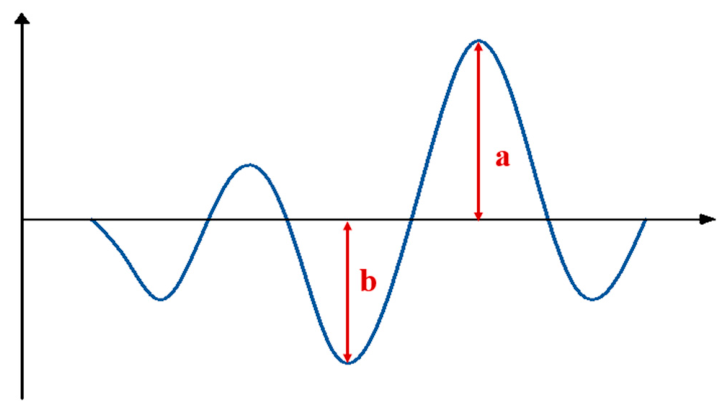
In the comparative analysis between the experimental and numerical results, the zero-crossing method was adopted for the time-domain analysis of vessel motions to obtain the statistical characteristics of the motion responses, as illustrated in Figure 7. The zero-to-peak criterion was employed to statistically analyze the time-domain results, including the maximum value, significant peak value, significant trough value, and standard deviation. Specifically, the maximum value is defined as the maximum value of a within the entire calculation time history; the significant peak value is defined as the average of the largest one-third values of a; and the significant trough value is defined as the average of the largest one-third values of b. The accuracy of the numerical calculation method was validated through comparisons of these four motion statistical parameters. Since the mooring lines are subjected only to tensile forces and no negative values occur, the statistical analysis of mooring line tensions considered only the mean value, maximum value, significant peak value, and standard deviation.

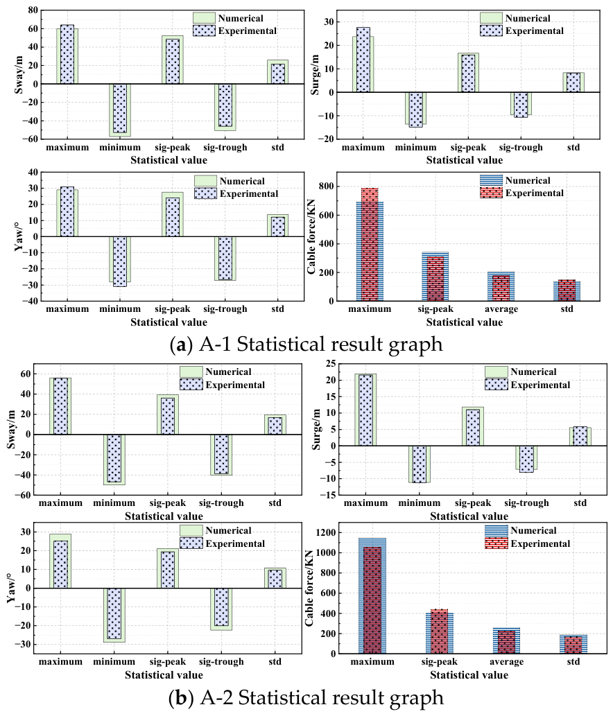
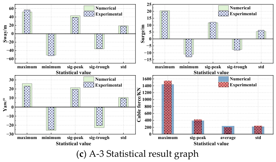
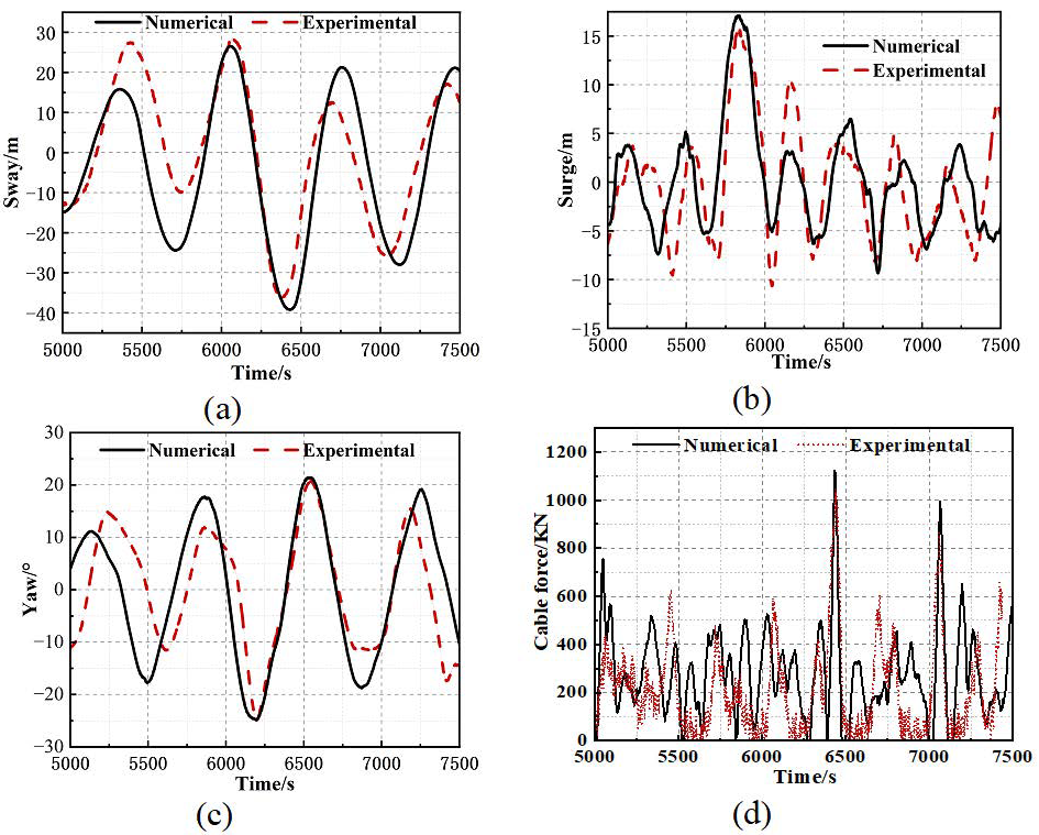
Based on the ocean environmental conditions listed in Table 3, the statistical comparison results between the numerical simulations and experimental measurements for the surge, sway, and yaw motions of the pile-supported single point mooring tanker, as well as the mooring line tensions, are presented in Figure 8. In addition, the comparisons of selected time-history curves under Condition A-2 are shown in Figure 9:

From the above comparisons of the time-history curves, it can be observed that certain discrepancies exist between the experimental and numerical results for both mooring line tensions and vessel motions. The primary reason is that the tanker moored by the pile-supported column-type single point mooring system exhibits relatively poor stability, making the vessel motions highly sensitive to environmental variations. Particularly under shallow-water conditions, the boundary layer near the basin bottom and fluid viscosity reduce the stability of shallow-water wave forms. As a result, the wave field environment within the vessel motion range under combined wind, wave, and current actions differs to some extent during the experiments. Regarding the flow field, the thickening of the bottom boundary layer together with wind-driven effects causes the fluid viscosity to produce a non-uniform flow velocity distribution, unlike the nearly uniform distribution typically observed in deep water. However, AQWA, which is based on potential flow theory, does not account for the variations induced by these viscous effects. These factors constitute the main sources of discrepancy between the experimental and numerical results. Nevertheless, from the overall comparison of the curves, the variation trends of the two sets of results are generally consistent. Moreover, the statistical comparisons indicate relatively small differences between the numerical and experimental results. For vessel motions, the maximum error among all statistical parameters does not exceed 14.58%, while for mooring line tensions, the maximum error does not exceed 14.7%. The results are presented in Table 4. These results demonstrate that the established numerical model possesses satisfactory accuracy and reliability and can therefore be applied to subsequent investigations on the hydrodynamic responses of pile-supported column-type single point mooring tankers.

Table 4. Error Data Table under Various Working Conditions.

Working Condition	A-1	A-2	A-3
Maximum displacement error	14.58%	12.75%	13.63%
Maximum tension error	14.70%	14.45%	14.32%

Table 4. Error Data Table under Various Working Conditions.

Working Condition	A-1	A-2	A-3
Maximum displacement error	14.58%	12.75%	13.63%
Maximum tension error	14.70%	14.45%	14.32%

2.4. Grid Independence Verification

The basic hull parameters adopted in the present calculation are listed in Table 1. Three loading conditions, namely ballast, partial load and full load, are defined for the designed hull displacement. In this section, the numerical model is validated mainly based on calculation results under the partial load draft condition, and the geometric model of the hull is presented in Figure 2.

Potential flow theory characterizes the flow field by solving the Laplace equation, whose numerical solution relies on the discretization of the continuous flow domain via meshes. Insufficient mesh density will cause distorted predictions of pressure distribution and wave loads; on the contrary, excessive mesh refinement will dramatically raise the computational cost. Grid convergence analysis is implemented to verify that once the mesh is refined beyond a certain threshold, the variations in key hydrodynamic parameters including motion response amplitudes, added mass and damping coefficients become negligible, which thereby confirms the grid independence of the computed results.

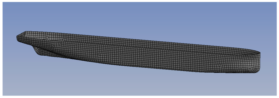
Hydrodynamic analyses in this paper are carried out using ANSYS AQWA, where the Hydrodynamic Diffraction module is utilized to conduct grid independence verification for numerical models with four distinct mesh schemes. Specific criteria must be followed during mesh generation, requiring a minimum of seven maximum mesh elements within each wavelength. With identical hull geometry and computational boundary conditions maintained, frequency-domain solutions are performed on four numerical models with mesh sizes of 1.5 m, 3 m, 4.5 m and 6 m, respectively. The convergence performance of meshes is assessed by comparing the resulting hull motion RAOs. The mesh discretization layout is illustrated in Figure 10.

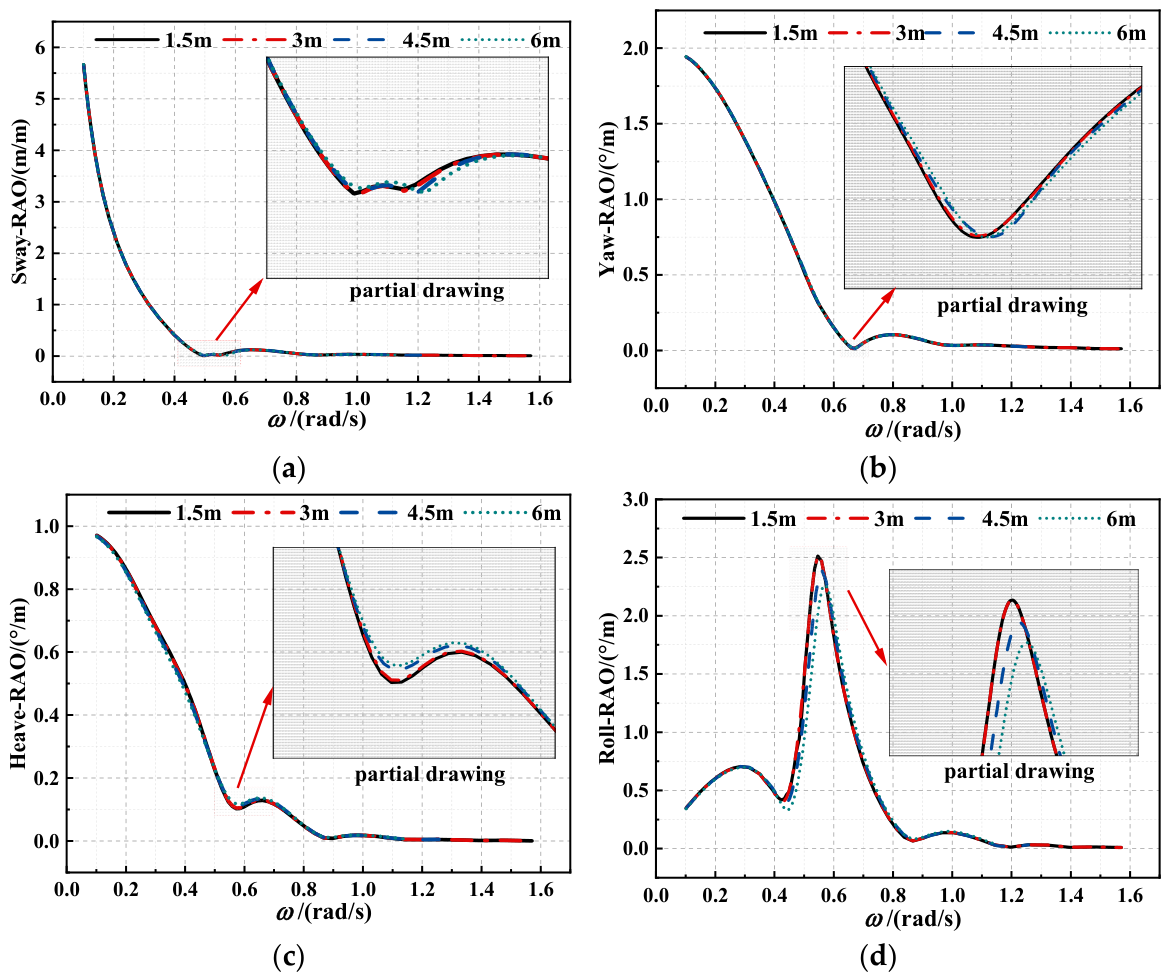
Grid independence verification in this section is performed based on motion RAOs of the hull in four degrees of freedom, namely sway, yaw, heave and roll. The calculated hull motion RAOs corresponding to meshes of different sizes are plotted in Figure 11. It can be observed from the motion RAOs of the four degrees of freedom that the overall variation trends of hull motion response curves under the four mesh sizes are basically consistent. Nevertheless, partial enlarged views reveal discrepancies among the calculation results near the peak and trough regions. In particular, obvious deviations exist in the maximum value of roll RAO and the corresponding natural frequency. By contrast, the response curves obtained with mesh sizes of 1.5 m and 3 m nearly overlap completely. To strike a balance between computational accuracy and efficiency, a mesh size of 3 m is adopted for all subsequent numerical calculations and analyses in this paper.

3. Analysis of the Effects of Shallow-Water Conditions on Vessel Hydrodynamic Parameters

In this chapter, frequency-domain analyses were conducted for the vessel at intermediate draft under six different water depth conditions: 13 m, 19 m, 30 m, 60 m, 100 m, and 500 m. The study aimed to obtain the variations in hydrodynamic parameters with different water-depth-to-draft ratios, including added mass, radiation damping, response amplitude operators (RAOs), and second-order wave force transfer functions.

3.1. Effect of Water Depth on Added Mass

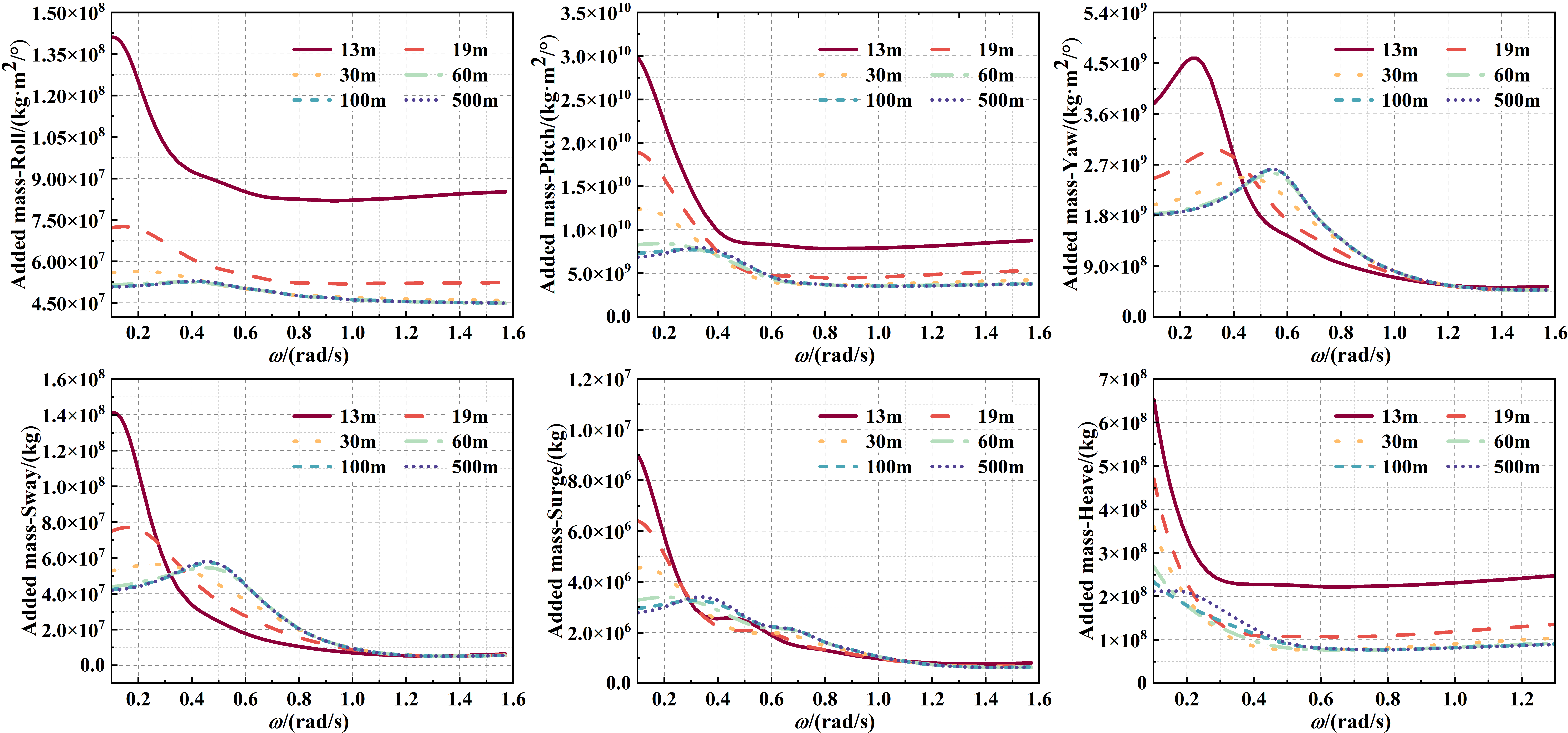
Under shallow-water conditions, the gap between the hull bottom and the seabed is reduced, constraining the flow space of the surrounding water. The water displaced by the vessel’s motion cannot smoothly circulate around the hull as it does in deep water; instead, it accumulates near the hull and accelerates with the vessel. This effect is equivalent to the vessel dragging a larger volume of water along with it, resulting in a significant increase in added mass (inertia). The degree of flow blockage varies with water depth and direction of motion, leading to differences in the increment of added mass, as shown in Figure 12.

The six-degree-of-freedom added mass results indicate that added mass in all directions exhibits clear dependence on both water depth and frequency: it gradually decreases with increasing frequency and stabilizes at high frequencies. Added mass increases significantly as water depth decreases, with shallow-water conditions (13 m and 19 m) showing markedly higher values than deeper water conditions (30 m, 60 m, 100 m, and 500 m). This difference is especially pronounced in the low-frequency range below 0.4 rad/s. When water depth exceeds 30 m, the added mass curves for different depths nearly coincide, indicating that shallow-water effects become negligible. Overall, the difference in added mass between shallow and deep water is most significant at low frequencies. At high frequencies, due to the limited fluid disturbance and reduced seabed influence, the added mass for different water depths gradually converges. However, at a water depth of 13 m, the added mass in roll, pitch, and heave directions still exhibits noticeable differences at high frequencies, whereas for the remaining three degrees of freedom, the added mass shows little variation with water depth when the frequency exceeds 1 rad/s.

3.2. Effect of Water Depth on Radiation Damping

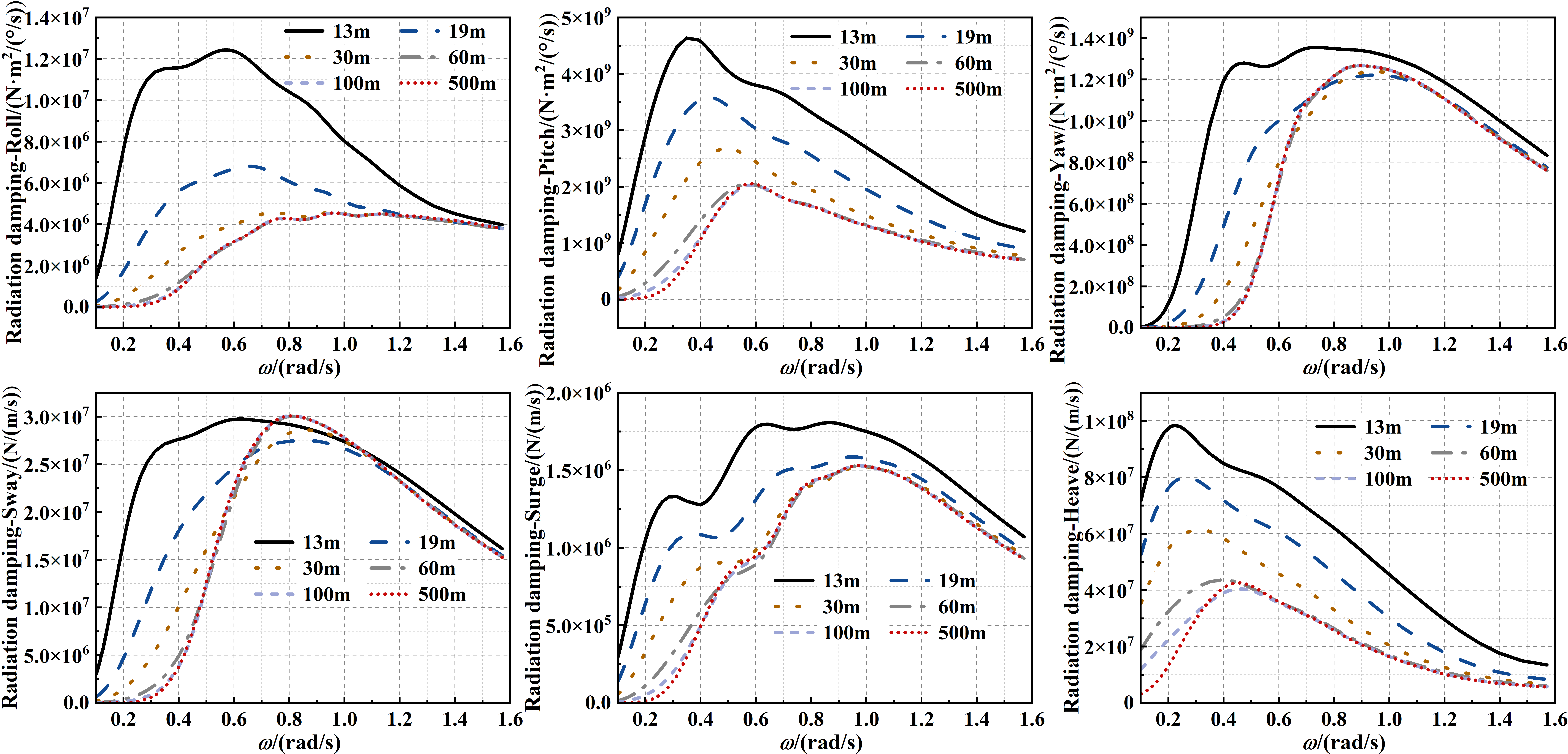
The radiation damping results of the vessel in six degrees of freedom under different water depth conditions are presented in Figure 13. The radiation damping in each degree of freedom exhibits clear frequency-dispersion characteristics with varying frequency, while the differences induced by water depth are mainly concentrated in the low- and medium-low-frequency regions. As the water depth decreases, the radiation damping curves generally show an earlier rise in the low-frequency range, a shift in the peak value toward lower frequencies, and variations in peak magnitude. When the water depth increases to 60 m and above, the results for all degrees of freedom nearly coincide, indicating that the shallow-water effect becomes significantly weakened and the hydrodynamic characteristics gradually approach those under deep-water conditions. These phenomena mainly result from the influence of shallow water on the generation and propagation of radiated waves. The seabed boundary restricts the vertical development of waves and compresses the energy radiation space. In addition, the shallow-water dispersion relationship reduces wave celerity and shortens wavelength, particularly hindering the outward propagation of low-frequency radiated waves. Meanwhile, multiple reflections and interference between the vessel and the seabed alter the pressure distribution on the vessel surface. Under the combined effects of these mechanisms, radiation damping in shallow water is generally larger than that in deep water, although local amplification may also occur near certain resonance frequencies.

3.3. Effect of Water Depth on RAOs (Response Amplitude Operators)

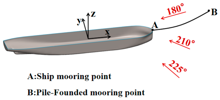
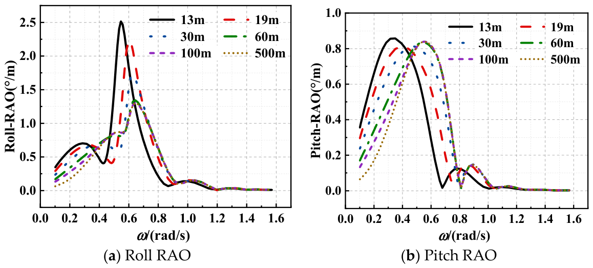
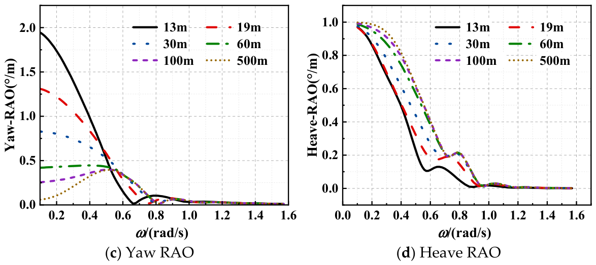
The RAO results of vessel motions under different water depths are shown in Figure 14. To ensure that all degrees of freedom exhibit measurable motion and considering that the angle between the waves and the vessel cannot remain constant during actual single-point mooring, this section analyzes the effects of shallow-water conditions on vessel motion RAOs with a wave-to-vessel incident angle of 225°.

It can be observed from Figure 14 that the RAOs of the vessel in all six degrees of freedom exhibit pronounced shallow-water effects under different water depths. Under oblique wave conditions, the roll and pitch motions show distinct resonance peaks, and the corresponding peak frequencies shift toward the low-frequency region as water depth decreases. Combined with the variation characteristics of added mass, it can be seen that the added mass in shallow water is significantly greater than that in deep water. According to the relationship governing natural frequency, when the overall restoring stiffness remains unchanged, an increase in added mass leads to a shift in the natural frequencies of roll and pitch motions toward lower frequencies. The influence of shallow-water effects on RAOs is mainly concentrated in the low-frequency region below 0.9 rad/s. When the water depth exceeds 60 m, the RAO curves for all degrees of freedom almost completely overlap across the entire frequency range, which is consistent with the variation pattern observed for radiation damping under shallow-water effects. For roll, pitch, and yaw motions, when the wave frequency is lower than 0.45 rad/s, shallower water depths correspond to larger RAO values; however, when the frequency exceeds 0.45 rad/s, the RAOs become smaller as the water depth decreases. Once the frequency is greater than 1.2 rad/s, the RAOs under all water depth conditions gradually approach zero. In contrast, the heave motion exhibits smaller RAO values under shallower water conditions throughout the entire frequency range. This is mainly because the confinement effect of the water between the seabed and the hull becomes stronger in shallow water, resulting in greater resistance to heave motion and consequently causing the heave RAO to remain consistently lower than the corresponding deep-water values.

3.4. Effect of Water Depth on QTFs (Quadratic Transfer Functions)

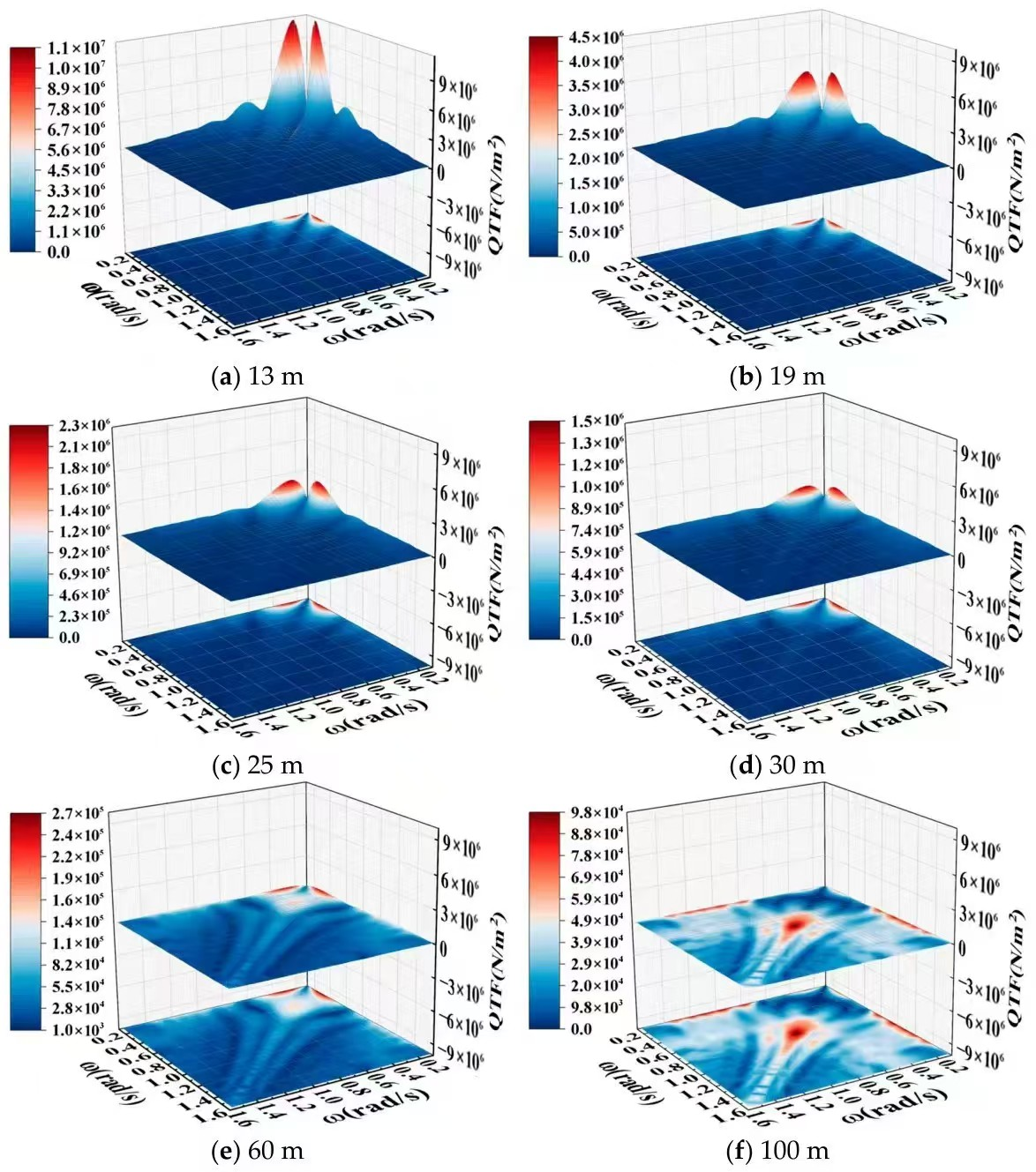
In this section, the Pinkster approximation and the Newman approximation were, respectively, employed to calculate the surge-direction QTF matrices of the vessel under head-wave conditions. The vessel draft condition was set to the intermediate loading condition, and the investigated water depths ranged from shallow to deep, namely 13 m, 19 m, 25 m, 30 m, 60 m, and 100 m. The QTF matrices obtained using the Pinkster approximation are shown in Figure 15:

The calculation results indicate that the shallower the water depth, the higher the QTF peak values: under the extremely shallow condition of 13 m, the main peak reaches approximately 1.1 × 10⁷ N/m², whereas it decreases to 9.8 × 10⁴ N/m² when the water depth increases to 100 m. In terms of morphology, for water depths less than 60 m, the QTF exhibits a typical double-peak pattern, with the peaks concentrated in the wave frequency range of 0.2–0.4 rad/s. The shallower the water, the more concentrated and sharper the peaks. As water depth increases, the peaks gradually broaden; at 60 m, two small double peaks remain in the low-frequency region, while mid-to-high frequency ranges begin to show additional peaks. The QTF distribution is primarily aligned along the frequency diagonal and decays symmetrically to both sides. When the water depth reaches 100 m, the double-peak pattern disappears, and a single main peak appears near 0.8 rad/s, with a more uniform distribution on either side of the diagonal.

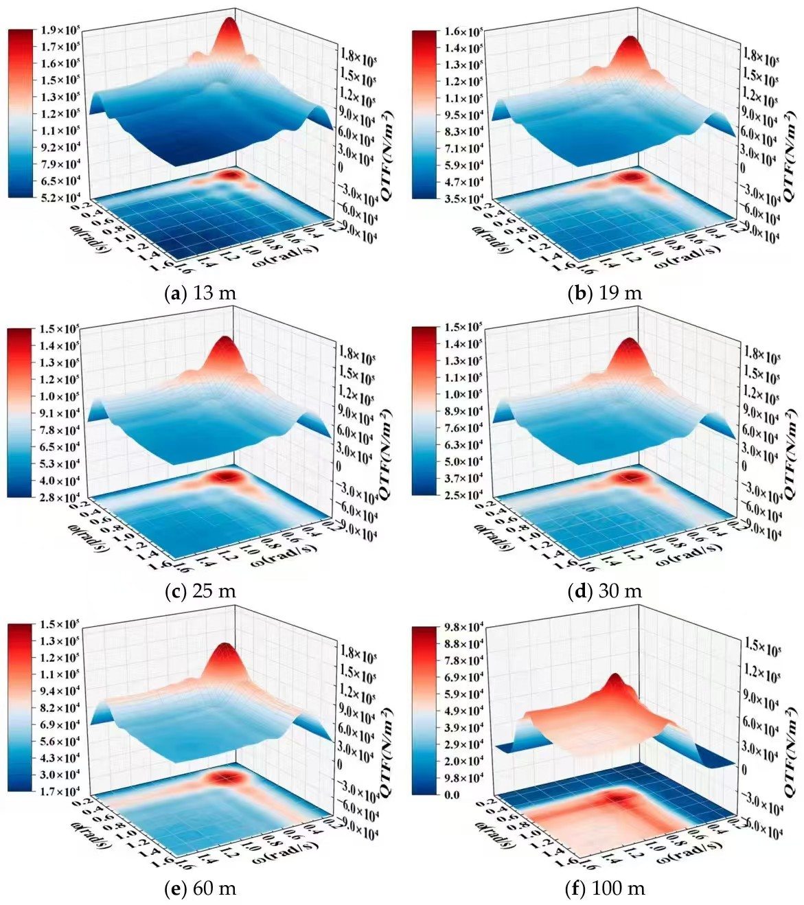
The QTF matrices calculated using the Newman approximation under different water depths are shown in Figure 16. Across the investigated depth range, all matrices exhibit a single-peak morphology, with peak values located along the diagonal and two primary frequency bands corresponding to the peak frequencies. Comparing water depths from 13 m to 100 m, it can be observed that shallower water causes the peak frequency to shift toward lower frequencies and increases the peak magnitude. At a depth of 100 m, both the peak magnitude and corresponding frequency show significant changes. In terms of distribution uniformity, as water depth increases, the QTF matrices tend to distribute more evenly between the two main frequency bands and the high-frequency region, a feature that is especially pronounced at a water depth of 100 m.

A comparison of the QTF matrices obtained using the Pinkster approximation indicates that, for water depths less than 30 m, the differences between the two methods are highly pronounced, and these differences increase as the water depth decreases. At a water depth of 30 m, the peak values of the QTF matrices calculated by the two methods differ by approximately an order of magnitude; when the depth decreases to 13 m, the difference increases to roughly two orders of magnitude. The primary reason for this phenomenon is that the Pinkster approximation accounts for both the interactions of first-order quantities and the effects of the second-order velocity potential when calculating the second-order difference-frequency force transfer function, thereby producing a complete QTF matrix. In contrast, the Newman approximation only considers the interactions of first-order quantities and constructs the QTF matrix accordingly, completely neglecting the contribution of the second-order velocity potential. Consequently, the QTF matrices obtained using the Newman approximation differ significantly from those obtained with the Pinkster approximation. This discrepancy becomes even more pronounced as the water depth decreases, because the contribution of the second-order velocity potential to the second-order forces increases, and the nonlinear effects of the waves become more significant. The Pinkster approximation captures these enhanced nonlinear interactions, further widening the differences in both QTF peak values and the corresponding frequencies between the two methods.

4. Analysis of the Effects of Shallow-Water Conditions on Vessel Hydrodynamic Performance

4.1. Investigation of Numerical Calculation Methods Under Shallow-Water Conditions

The previous section presented the differences in the QTF matrices obtained using the Pinkster approximation and the Newman approximation under various water depth conditions. Although the Pinkster approximation can provide a more accurate evaluation of second-order wave forces, it involves relatively high computational complexity and requires substantial computational resources. In contrast, while the Newman approximation does not explicitly account for the influence of difference-frequency terms in the calculation of second-order forces, it significantly reduces the computational effort by constructing the QTF matrix through a diagonal averaging approach. As water depth increases, the influence of the second-order velocity potential on the vessel gradually diminishes. Once the water depth reaches a certain level, the interaction effects associated with the first-order velocity potential become sufficient to represent the overall wave field effects. Meanwhile, increasing water depth also substantially weakens wave nonlinearity. Therefore, beyond a certain critical water depth, the results obtained using the Newman approximation become essentially consistent with those calculated using the Pinkster approximation. Above this critical depth, the Newman approximation can be adopted to account for the effects of second-order wave forces on the vessel.

However, existing studies rarely address this critical water depth issue, and available research indicates that the critical depth varies with vessel type and draft condition. In this section, the vessel draft (d) and corresponding water depth (h) are converted into a dimensionless parameter, namely the water-depth-to-draft ratio (h/d). For the ballast, intermediate loading, and fully loaded conditions of the tanker, time-domain analyses of the hydrodynamic performance of the pile-supported single point mooring tanker were conducted under different h/d conditions using both the Newman approximation and the Pinkster approximation. By analyzing the variations in vessel motions and mooring line tensions, the critical water depths requiring consideration of the two calculation methods under different loading conditions were determined. The ocean environmental condition adopted in this section corresponds to Condition A-3, and the associated water-depth-to-draft ratios are listed in

Table 5. Table of Water Depth Parameters for Different Draft Conditions.

Parameter	Draft/m	Water Depth/m	Corresponding Water-Depth-to-Draft Ratio
	Ballast Condition (6.910)	9.041, 11.127, 13.213, 15.299 17.386, 19.472, 20.863, 41.727	1.31, 1.61, 1.91 2.21, 2.51, 2.81 3.02, 6.04
	Intermediate Loading Condition (9.936)	13, 16, 19, 22, 25, 28, 30, 60
	Fully Loaded Condition (11.166)	14.601, 17.971, 21.341, 24.710 28.079, 31.449, 33.695, 67.391

.

(1) Calculation of the Critical Water-Depth-to-Draft Ratio Under Ballast Draft Condition

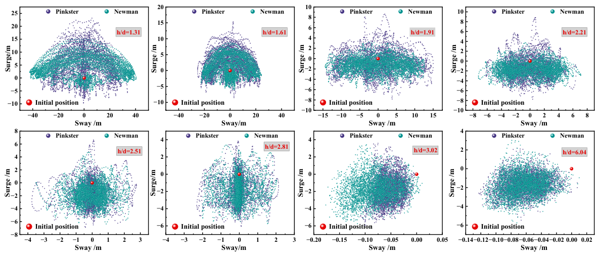
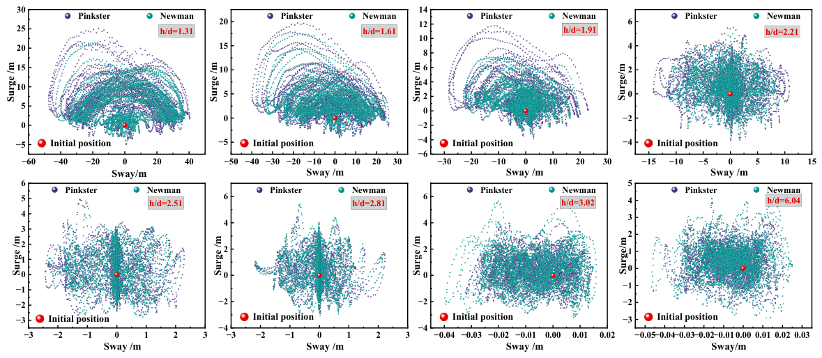
For the ballast condition, the vessel’s planar motions corresponding to different water-depth-to-draft ratios are shown in Figure 17. It can be observed that the overall differences in vessel planar motions calculated using the Pinkster and Newman approximations are minor. From the trajectory of the vessel’s center of gravity, when the water-depth-to-draft ratio is less than 2.81, the difference in sway motion between the two methods is very small; however, in the surge direction, the surge motion predicted by the Pinkster approximation is slightly larger than that obtained using the Newman approximation. When the water-depth-to-draft ratio exceeds 2.81, the vessel exhibits negligible sway motion, with only some surge motion remaining. Regarding the pitch motion, when the water-depth-to-draft ratio is less than 2.51, the Pinkster approximation predicts the onset of pitch motion earlier, and after motion stabilizes, the maximum roll angle obtained using the Pinkster approximation is slightly higher than that calculated by the Newman method. When the water-depth-to-draft ratio reaches 2.51, the results of the two methods are essentially consistent.

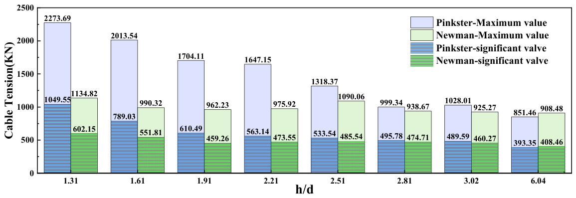
The calculated maximum and significant values of mooring line tensions under different water-depth-to-draft ratios are shown in Figure 18:

According to the calculated mooring line tensions under the ballast condition, when the water-depth-to-draft ratio is less than 3.02, the mooring line tensions obtained using the Pinkster approximation are consistently greater than those calculated using the Newman approximation, regardless of whether the maximum values or significant values are considered. Moreover, the discrepancy between the two methods becomes increasingly pronounced as the water depth decreases. Combined with the vessel motion analysis, the primary reason for this discrepancy is that the Pinkster approximation predicts a larger surge motion range. The stronger surge motion induces greater pulling forces on the mooring lines, thereby resulting in larger differences in mooring line tensions, and this difference further increases with decreasing water depth. When the water-depth-to-draft ratio decreases to 2.81, the differences between the two methods become relatively small, remaining within 6%. In conjunction with the motion response results under different water-depth-to-draft ratios, it can also be observed that the vessel motion responses predicted by the two methods are essentially consistent at a ratio of 2.81. Therefore, for the ballast condition, the critical water-depth-to-draft ratio at which significant differences arise between the two calculation methods can be identified as 2.81. When the water-depth-to-draft ratio is lower than this value, the results obtained using the Pinkster approximation are considered to better represent the actual physical conditions and are therefore more beneficial for ensuring the safety of mooring system design. Conversely, when the water-depth-to-draft ratio exceeds 2.81, the results obtained by the two methods become essentially consistent, and the computationally more efficient Newman approximation can be adopted.

In addition, it can be observed from the figure that the results obtained using the Newman approximation vary only slightly regardless of the water-depth-to-draft ratio, whereas the results obtained using the Pinkster approximation change significantly with increasing water-depth-to-draft ratio and gradually stabilize once the critical depth is reached. This phenomenon is consistent with the QTF calculation results under different water depths: the QTF matrices obtained using the Pinkster approximation vary significantly with increasing water depth, while the variations in the Newman approximation results are relatively small.

(2) Calculation of the Critical Water-Depth-to-Draft Ratio Under Intermediate Loading Condition

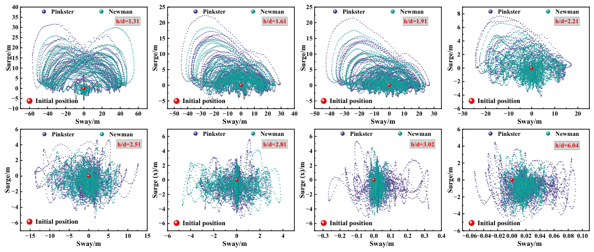
For the intermediate loading condition, the vessel motion trajectories under different water-depth-to-draft ratios are shown in Figure 19. From the motion trajectory results, it can be observed that when the water-depth-to-draft ratio is less than 2.51, the range of the vessel’s center-of-gravity motion calculated using the Pinkster method is larger than that obtained using the Newman approximation, both in terms of planar motion trajectories and roll amplitudes, with the discrepancy in the sway direction being particularly pronounced. When the water-depth-to-draft ratio reaches 2.51, the motion trajectories predicted by the two calculation methods are essentially consistent, and when the ratio exceeds 2.81, the vessel exhibits almost no oscillatory motion.

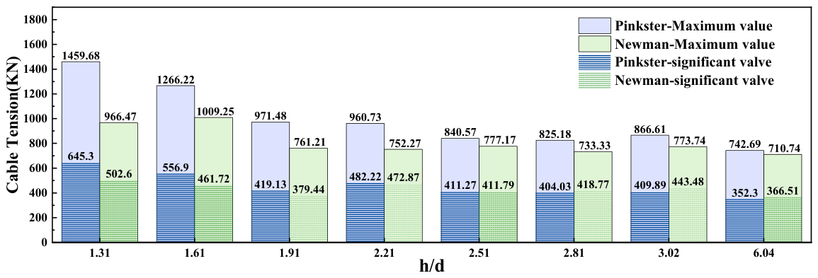
Under the intermediate loading condition, the maximum and significant mooring line tensions at different water-depth-to-draft ratios are presented in Figure 20.

It can be observed from the mooring line tension results under the intermediate loading condition that the variation trend between the two calculation methods is consistent with that under the ballast condition, namely that the results obtained using the Newman approximation are smaller than those calculated using the Pinkster approximation. However, unlike the ballast condition, the discrepancy between the two methods under the intermediate loading condition is less pronounced. Combined with the comparative analysis of vessel motions, it can be concluded that under the intermediate loading condition, the primary differences between the two methods are reflected in the sway motion response, whereas under the ballast condition, the differences mainly occur in the surge direction. This indicates that although sway motion can induce certain pulling effects on the mooring lines, its influence on mooring line tension is less significant than that caused by surge motion. According to the calculation results shown above, the critical water-depth-to-draft ratio for the intermediate loading condition is determined to be 2.51.

(3) Calculation of the Critical Water-Depth-to-Draft Ratio Under Fully Loaded Condition

Fully Loaded–Vessel Motion Trajectories at Different Water-Depth-to-Draft Ratios (Figure 21).

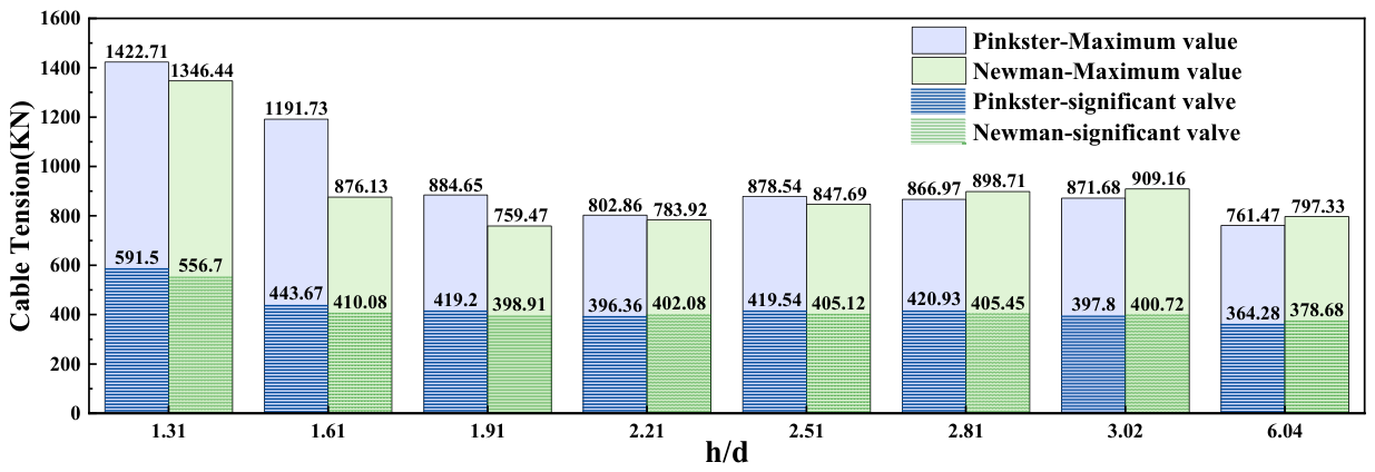
According to the calculation results under the fully loaded condition, the variation characteristics of vessel motions are very similar to those observed under the intermediate loading condition. The differences between the motion responses predicted by the two calculation methods are also mainly reflected in the sway direction. However, these differences gradually decrease as the water-depth-to-draft ratio increases, and when the ratio reaches 3.02, the vessel exhibits almost no oscillatory motion. Unlike the ballast and intermediate loading conditions, however, the fully loaded condition does not present a distinct critical water-depth-to-draft ratio that can be directly identified from the motion response perspective alone. Therefore, the critical water depth should be determined in conjunction with the mooring line tension results.

The mooring line tension results calculated using the Pinkster approximation and the Newman approximation under different water-depth-to-draft ratios for the fully loaded tanker are shown in Figure 22.

It can be observed from the figure that under the fully loaded condition, the differences in mooring line tension responses obtained using the two calculation methods are relatively small. Moreover, when the water-depth-to-draft ratio reaches 2.21, the mooring line tension results predicted by the two approximation methods become essentially consistent. Therefore, for the fully loaded condition, the critical water-depth-to-draft ratio corresponding to the two calculation methods can be identified as 2.21. When the actual water depth exceeds this critical value, the Newman approximation can be adopted to evaluate the effects of second-order wave forces on the mooring system.

4.2. Study on the Hydrodynamic Response of a Ship Hull Under Different Water-Depth-to-Draft Ratios

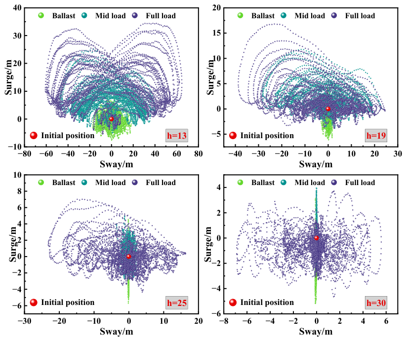
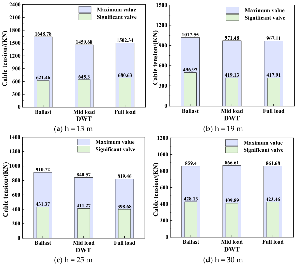
From the above study on the critical water-depth-to-draft ratio based on different calculation methods, it can be seen that, regardless of the numerical method adopted, the pile-supported single point mooring tanker will exhibit low-frequency slow-drift motions in the horizontal plane under shallow-water conditions. This section mainly focuses on the water-depth range of the design area for the pile-supported single point mooring system, and carries out a comparative study on the hull motion responses and mooring line tensions under different loading conditions at the same water depth. The calculated water depths and loading conditions are shown in

Table 6. Table of Calculation Cases for Different Water-Depth-to-Draft Ratios.

Parameters	Draft/m	Water Depth/m	Corresponding Water-Depth-to-Draft Ratio
	Ballast Condition (6.910)	13, 19, 25, 30	1.88, 2.75, 3.62, 4.34
	Intermediate Loading Condition (9.936)		1.31, 1.91, 2.51, 3.02
	Fully Loaded Condition (11.166)		1.16, 1.70, 2.24, 2.69

.

The trajectories of ship motions in the horizontal plane calculated under the above four water depths and different loading conditions are shown in Figure 23. Under the same water depth, a larger ship draft leads to a greater oscillation amplitude in the horizontal plane, and this difference is particularly pronounced in the sway and yaw directions. However, in terms of the surge motion amplitude, a smaller ship draft corresponds to a smaller negative motion amplitude, indicating that the ship moves farther away from the pile-supported jacket in the x-direction. Meanwhile, when the water depth reaches 25 m, the ship under the medium-load and ballast draft conditions shows almost no obvious oscillation. In contrast, under the full-load draft condition, a certain degree of oscillation still occurs even when the water depth reaches 30 m. Therefore, for the pile-supported single-point mooring system operating within the designed regional water-depth range, when the full-load draft operating condition is considered, more attention should be paid to the analysis of ship motions under this draft condition, as well as to the corresponding oscillation suppression measures.

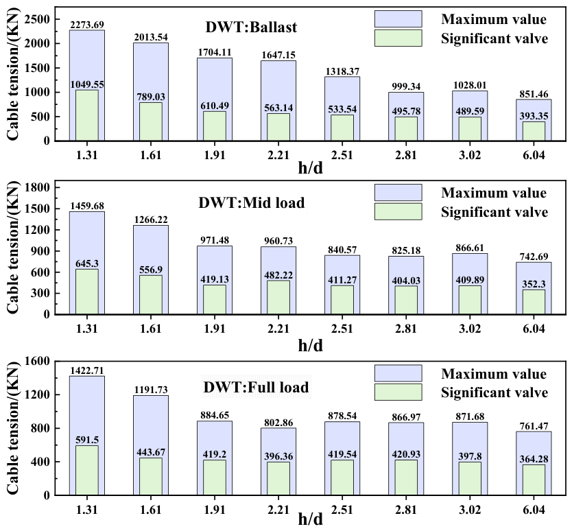
The calculated results of mooring line tension under different water-depth-to-draft ratios are shown in Figure 24. It can be seen that, regardless of the variation in ship draft, the mooring line tension decreases with increasing water depth. Combined with the motion response results, this indicates that the shallower the water depth, the larger the ship motion amplitude, and consequently the greater the mooring line tension induced by the motion. As shown in the figure, when the water depth is less than 25 m, the mooring line tension under the ballast draft condition is slightly greater than that under the other two loading conditions. By comparing the motion responses, it can be found that, under shallow-water conditions, when the ship is in the ballast draft condition, its surge motion away from the pile-supported jacket is larger than that under the other two loading conditions. Moreover, the shallower the water depth, the farther the ship moves away from the pile-supported jacket. The effective pulling effect on the mooring lines caused by this offset is greater than that caused by the ship oscillation, resulting in a slightly larger mooring line tension under the ballast draft condition than under the other two loading conditions.

4.3. Study on the Hydrodynamic Response of the Ship Hull Under the Same Water-Depth-to-Draft Ratio

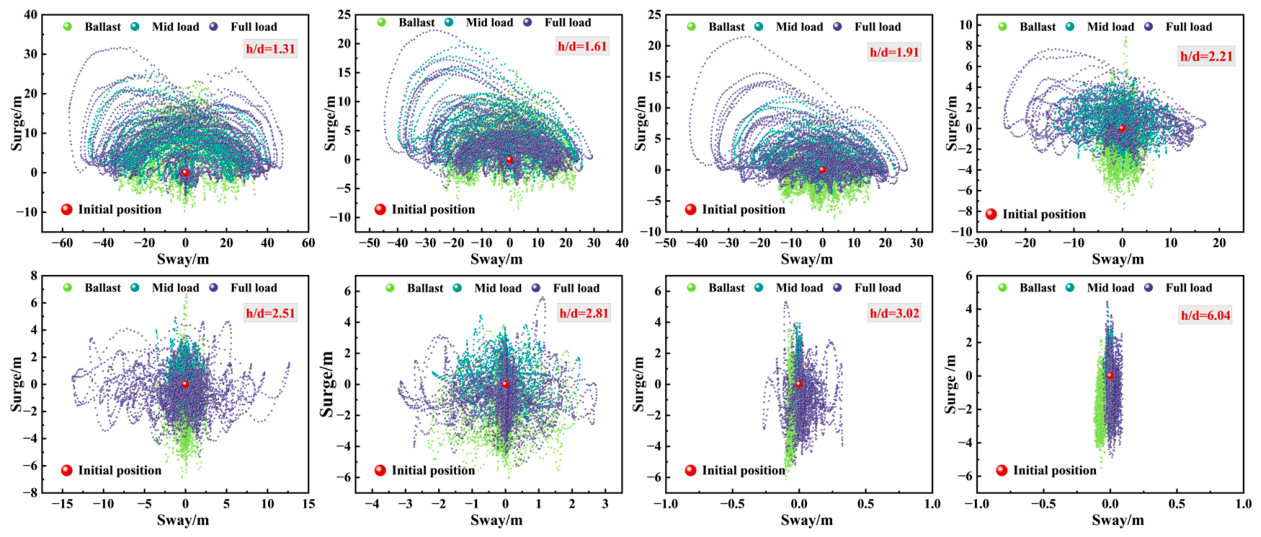
It can be seen from the above calculation results under different water-depth-to-draft ratios that, under the same water depth, both the mooring line tension and ship motions show certain differences under different loading conditions. Since the shallow-water effect is closely related to the water-depth-to-draft ratio of the ship, this section mainly investigates the dynamic response characteristics of the ship under shallow-water effects for different loading conditions while maintaining the same water-depth-to-draft ratio. The calculation cases are listed with reference to Table 5.

The motion trajectories under different loading conditions and different water-depth-to-draft ratios are shown in Figure 25.

According to the above motion calculation results, under the same water-depth-to-draft ratio, the ship motions in the sway direction show obvious differences among different draft conditions. With the increase in draft, the ship presents a wider motion range in the sway direction within the horizontal plane. In addition, its motion trajectory is not completely symmetrical, and the motion range in the negative y-direction is larger. Meanwhile, it can also be seen from the figure that the motion follows a similar trend to that observed under different water-depth-to-draft ratios; that is, under the ballast draft condition, the ship tends to move farther away from the pile-supported jacket in the surge direction. When the water-depth-to-draft ratio is less than 2.51, the smaller the draft, the faster the ship motion attenuates with the increase in the water-depth-to-draft ratio. When the water-depth-to-draft ratio reaches 2.81, the ship motions under the three draft conditions become basically consistent. After the water-depth-to-draft ratio reaches 3.02, the ship basically no longer exhibits obvious oscillation.

The calculated results of mooring line tension under the same water-depth-to-draft ratio and different loading conditions are shown in Figure 26. It can be seen from the figure that, when the water-depth-to-draft ratio is the same, the mooring line tension under the ballast draft condition is greater than that under the other two loading conditions. This difference becomes more obvious, especially when the water-depth-to-draft ratio is smaller. Combined with the motion analysis, the main reason for this difference is still that, under shallow-water conditions, the ship under the ballast draft condition is more likely to move away from the pile-supported jacket in the surge direction, resulting in a more significant dragging effect on the actual mooring line tension. For the medium-load and full-load conditions, when the water-depth-to-draft ratio is less than 2.21, the mooring line tension under the medium-load draft condition is slightly greater than that under the full-load draft condition. When the water-depth-to-draft ratio reaches 2.51, the difference between the two becomes very small.

4.4. Analysis of the Critical Water Depth for Ship Hull Grounding

Since the pile-supported single point mooring system studied in this thesis mainly operates in shallow or even extremely shallow water areas, the clearance between the ship bottom and the seabed is relatively small. Under the action of the marine environment, the heave and rotational motions of the tanker may cause the hull to collide with the seabed, leading to the occurrence of grounding. Therefore, for a moored tanker operating in shallow-water areas, it is necessary to investigate the grounding problem so as to avoid collision between the hull and the seabed, prevent structural damage, and ensure the operational safety of the whole mooring system. Based on the calculation results of the three loading conditions under different water-depth-to-draft ratios discussed above, this section conducts a statistical analysis of the minimum clearance between the hull and the seabed and determines the critical water depth for grounding under the three loading conditions.

(1) Selection of Reference Points for Tanker Bottom Grounding

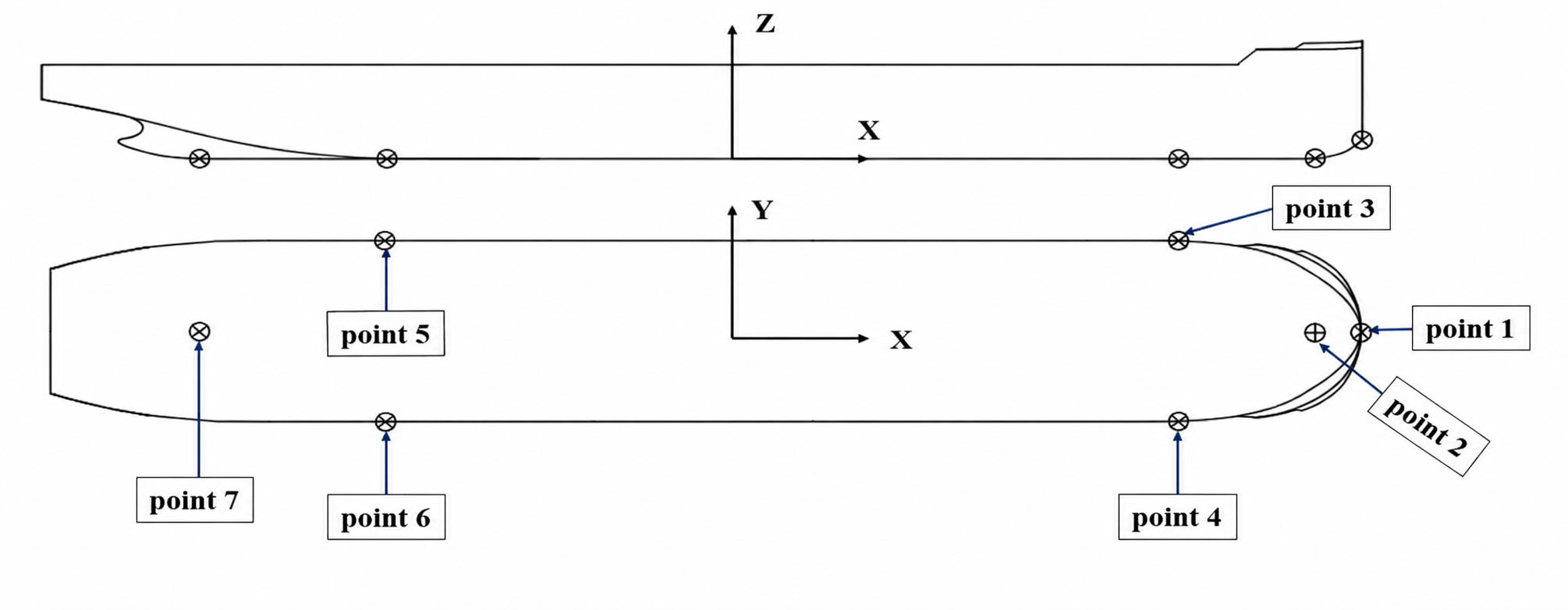
In a single-point moored ship, the intersections between the bow, the stern, and the parallel midbody are generally considered to be the most common locations where grounding is likely to occur. Therefore, a total of seven grounding reference points are selected on the hull in this thesis. Among them, four reference points are located at the intersections between the fore and aft parts of the parallel midbody. Based on the geometric characteristics of the hull, one additional reference point is selected at the stern, and two reference points are selected at the bow. The schematic diagram of the reference points is shown in Figure 27.

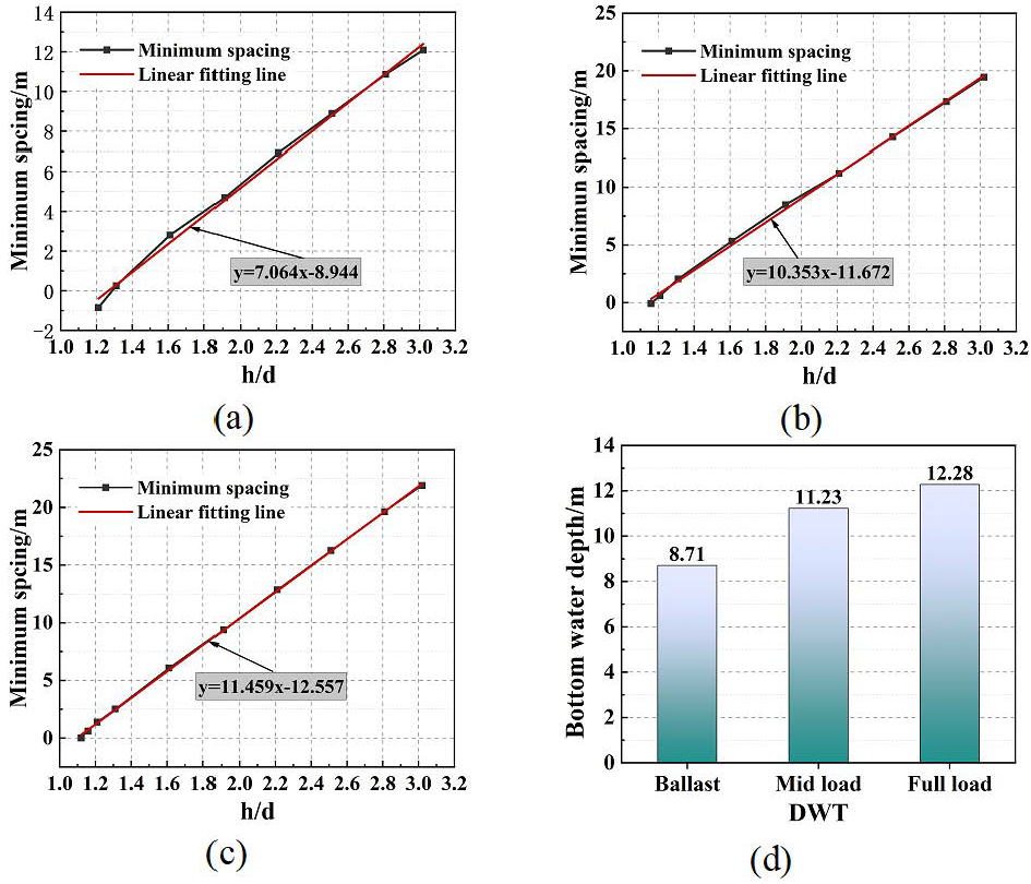
According to existing studies, for a single-point moored tanker, grounding problems are often caused by the combined action of wind, waves, and current in the marine environment. Therefore, it is necessary to carry out a time-domain analysis for the pile-supported column-type single point mooring system. Referring to the operating conditions listed in Table 5 and A-3, this section statistically analyzes the minimum clearance between the hull and the seabed under different water-depth-to-draft ratios, and further calculates and analyzes the critical water depth for grounding under the three loading conditions. The minimum clearances between the hull and the seabed under different water-depth-to-draft ratios for the three loading conditions are shown in Figure 28.

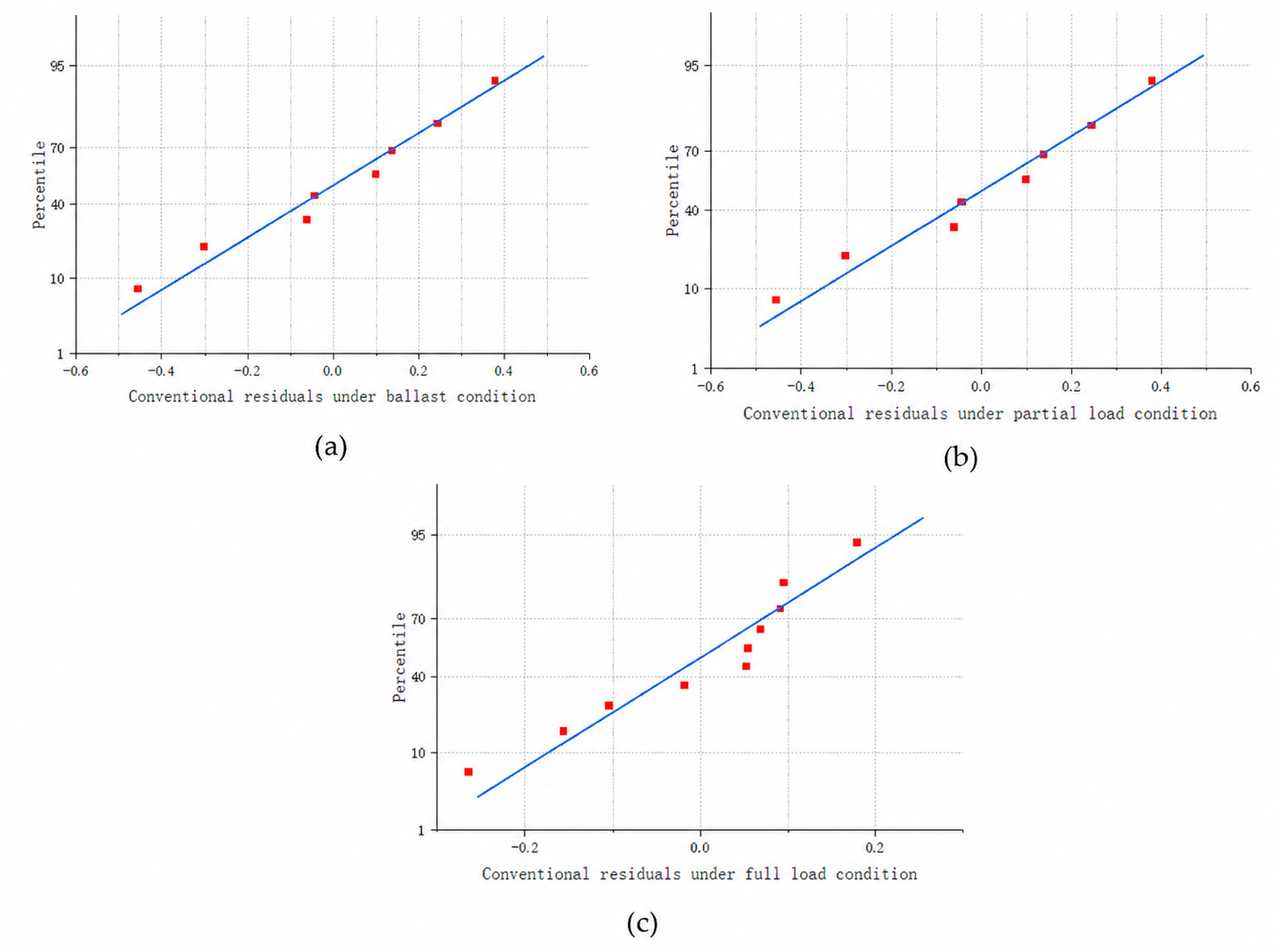
The relevant parameters of the fitting equations illustrated in the above figure are listed as follows: the coefficient of determination $R^2$ equals 0.99876 under the partial load condition, 0.99973 under the full load condition, and 0.99666 under the ballast condition. The corresponding residual plots are shown in Figure 29.

Figure 29. Normal Quantile-Quantile Plot. (a) Normal Q-Q Plot under ballast condition. (b) Normal Q-Q Plot under partial load condition. (c) Normal Q-Q Plot under full load condition.

Figure 29. Normal Quantile-Quantile Plot. (a) Normal Q-Q Plot under ballast condition. (b) Normal Q-Q Plot under partial load condition. (c) Normal Q-Q Plot under full load condition.

Figure 26 present the minimum clearance between the hull and the seabed under different water-depth-to-draft ratios for the three draft conditions, together with the corresponding fitted lines. It can be seen from the figures that, regardless of the loading condition, there is a strong linear relationship between the minimum clearance between the hull and the seabed and the water-depth-to-draft ratio. The fitted lines further indicate that the slope of the fitted line increases with increasing draft. As shown in the figures, the critical water-depth-to-draft ratios for grounding under the full-load, medium-load, and ballast draft conditions are 1.10, 1.13, and 1.26, respectively. This result indicates that the greater the ship loading, the smaller the corresponding critical water-depth-to-draft ratio for grounding. Figure 28d shows the corresponding critical water depths for grounding under different loading conditions.

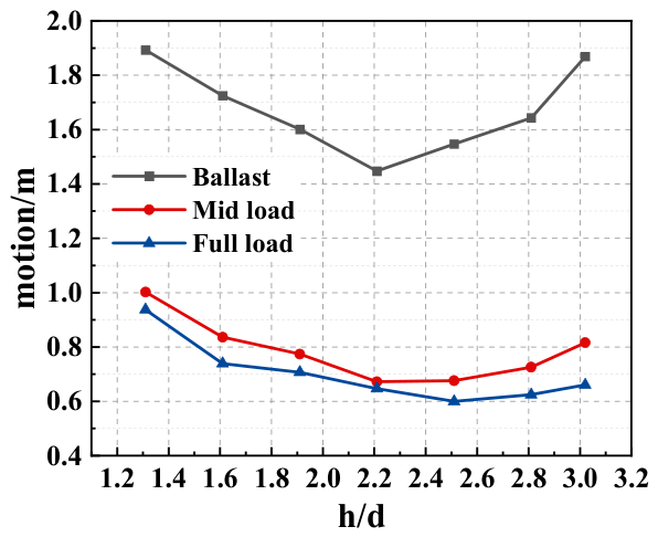
It can also be observed from the above figures that, under the same water-depth-to-draft ratio, the minimum clearance between the hull and the seabed during the whole motion time history increases with increasing draft. One reason is that, under the same water-depth-to-draft ratio, a larger draft corresponds to a greater initial clearance between the hull and the seabed. Another reason is that, for this ship hull in shallow-water areas, under the same water-depth-to-draft ratio, a larger draft leads to a larger waterplane area, which results in greater resistance to heave, roll, and pitch motions. Therefore, the vertical motion amplitude under the same water-depth-to-draft ratio is smaller than that under lighter loading conditions. This phenomenon can also be reflected in Figure 30, which shows the reduction in hull–seabed clearance caused by ship motions under different water-depth-to-draft ratios.

It can be seen from Figure 30 that, under the same water-depth-to-draft ratio, the vertical motion amplitude under the full-load condition is smaller than that under the other two loading conditions, which leads to a smaller critical water-depth-to-draft ratio for grounding. Moreover, the larger the difference in draft, the more obvious this difference becomes. Under the three loading conditions, the maximum vertical motion amplitude of the ship hull first decreases and then increases as the water-depth-to-draft ratio decreases. The turning point corresponding to the full-load draft condition occurs between 2.2 and 2.5, while those for the medium-load and ballast draft conditions are around 2.2. The main reason for this variation trend is still related to the shallow-water effect. As the water-depth-to-draft ratio decreases, the shallow-water effect gradually reduces the ship motions in roll, pitch, and heave. However, when the water-depth-to-draft ratio decreases to a certain extent, the shallow-water effect may induce low-frequency motions in these three directions, and the low-frequency components may become significantly larger than the wave-frequency components, resulting in an increase in the vertical motion amplitude of the ship hull.

5. Conclusions

Based on the numerical method validated by model tests, this chapter investigates the shallow-water effect characteristics of the pile-supported single point mooring system. Through frequency-domain and time-domain analyses, the hydrodynamic performance of the ship hull under different water-depth-to-draft ratios (h/d) is quantitatively evaluated. The main conclusions are as follows:

(1)

Variation characteristics of hydrodynamic parameters: The added mass and radiation damping increase as the water depth decreases, with particularly significant variations in the low-frequency range, while the influence in the high-frequency range is relatively limited. When the water depth is greater than 60 m, the shallow-water effect basically disappears, and the curves of each degree of freedom tend to become consistent.

(2)

Motion RAO responses: The shallow-water effect has a significant influence on the six-degree-of-freedom motion RAOs. Under oblique waves, the roll and pitch motions show obvious resonance peak characteristics, and the peak frequency shifts toward the low-frequency range as the water depth decreases. When the water depth exceeds 60 m, the RAOs become consistent with those in deep water. In different frequency ranges, the influence of shallow water on the RAOs shows different trends: in the low-frequency range, the shallower the water depth, the larger the RAO; in the middle-frequency range, the opposite trend is observed; and in the high-frequency range, the RAOs tend to approach zero. The heave motion decreases as the water depth becomes shallower over the whole frequency range, which is mainly because shallow water limits the vertical diffusion of the fluid.

(3)

Second-order wave force transfer function (QTF): Whether the Newman approximation or the Pinkster approximation is adopted, the QTF matrix decreases with increasing water depth. Under shallow-water conditions, the results of the low-frequency difference-frequency components obtained by the Pinkster approximation are much larger than those obtained by the Newman approximation, and the difference increases significantly as the water depth decreases.

(4)

Critical water depth for the Newman and Pinkster approximations: Under the ballast condition, the overall differences between the two methods in terms of horizontal-plane motions are not significant. However, as the draft increases, the difference in the sway direction gradually becomes more obvious. In shallow water, the mooring line tension calculated by the Pinkster approximation is always larger than that calculated by the Newman approximation. When the water-depth-to-draft ratio reaches the critical value, the motion and tension results obtained by the two methods become basically consistent. The critical h/d values are 2.81 for the ballast condition, 2.51 for the medium-load condition, and 2.21–2.51 for the full-load condition.

(5)

Effects of loading condition and water depth: Under the same water depth, the mooring line tension under the ballast draft condition is the largest and is significantly higher than that under the other loading conditions. The mooring line tensions under all three loading conditions decrease with increasing water depth. The motion amplitude under the full-load draft condition is the largest. When the water depth reaches 30 m, the ship under the ballast and medium-load conditions basically shows no obvious oscillation, while the ship under the full-load condition still exhibits a certain degree of oscillation. The same trend is also observed under the same h/d. The difference in mooring line tension is mainly caused by the larger surge motion of the ship away from the pile foundation under the ballast condition, which enhances the dragging effect on the mooring lines.

(6)

Critical water depth for grounding: As the draft increases, the critical water-depth-to-draft ratio for grounding decreases. The critical water depths for grounding under the ballast, medium-load, and full-load conditions are 8.71 m, 11.23 m, and 12.28 m, respectively.

References

1. Khor, L.H.; Barltrop, N.D.P. A method of analysis for the extreme response of an offshore floating and weathervaning platform subjected to wave, current and wind from different directions. Underw. Technol. 1999, 24, 11–17. [Google Scholar] [CrossRef] [Scilit]
2. Wang, H.F.; Yang, X.L.; Zhang, S.S.; Liu, G.; Chen, Y.; Li, Z.; Zhao, Q.; Wu, J.; Huang, T.; Xu, F.; et al. Development status and suggestions for independent development of single point mooring systems. China Offshore Oil Gas. 2025, 37, 247–258. (In Chinese) [Google Scholar]
3. Newman, J.N. The drift force and moment on ships in waves. J. Ship Res. 1967, 11, 51–60. [Google Scholar] [CrossRef] [Scilit]
4. Pinkster, J.A.; van Oortmerssen, G. Computation of the first and second order wave forces on oscillating bodies in regular waves. In Proceedings of the 2nd International Conference on Numerical Ship Hydrodynamics, Berkeley, CA, USA, 19–21 September 1977. [Google Scholar]
5. Drake, K.R. An analytical approximation for the horizontal drift force acting on a deep draught spar in regular waves. Ocean Eng. 2011, 38, 810–814. [Google Scholar] [CrossRef] [Scilit]
6. Chang, S.; Huang, W.; Liu, F.; Song, H. Influence of second-order wave force and focusing position on dynamic responses of tension leg platform under a freak wave. Ocean Eng. 2021, 242, 110126. [Google Scholar] [CrossRef] [Scilit]
7. Carmo, L.H.; Simos, A.N. On the complementarity of the slender-body and Newman’s approximations for difference-frequency second-order wave loads on slender cylinders. Ocean Eng. 2022, 259, 111905. [Google Scholar] [CrossRef] [Scilit]
8. Li, S.; Fu, S.; Zhang, S.; Moan, T. Second-order hydroelastic analysis of a flexible floating structure under spatially inhomogeneous waves. Mar. Struct. 2022, 86, 103306. [Google Scholar] [CrossRef] [Scilit]
9. Park, B.W.; Yuck, R.H.; Cho, S.K.; Lee, J.H.; Kim, Y.S.; Park, J.C.; Jeong, W.M.; Kim, H.S.; Ha, M.K.; Kwon, S.J.; et al. The dynamic response of a moored vessel in shallow water using Boussinesq equations. In Proceedings of the ASME 2009 28th International Conference on Ocean, Offshore and Arctic Engineering (OMAE 2009), Honolulu, HI, USA, 31 May–5 June 2009; pp. 391–399. [Google Scholar]
10. Pessoa, J.; Fonseca, N. Investigation of depth effects on the wave exciting low frequency drift forces by different approximation methods. Appl. Ocean Res. 2013, 42, 182–199. [Google Scholar] [CrossRef] [Scilit]
11. Zhang, L.; Shi, W.; Karimirad, M.; Jiang, Z.; Yang, Y.; Wang, Z.; Li, X.; Chen, Y.; Zhao, Q.; Wu, T.; et al. Second-order hydrodynamic effects on the response of three semisubmersible floating offshore wind turbines. Ocean Eng. 2020, 207, 107371. [Google Scholar] [CrossRef] [Scilit]
12. Yang, J.; He, Y.P.; Zhang, Y.S.; Li, J.; Wang, H.; Liu, Z.; Chen, G.; Zhou, D.; Xu, F.; Wu, S.; et al. Experimental and numerical studies on the low-frequency responses of a spar-type floating offshore wind turbine. Ocean Eng. 2021, 222, 108571. [Google Scholar] [CrossRef] [Scilit]
13. Huo, P.; Wang, D.J.; Li, K.; Zhang, M.; Chen, X.; Liu, Y.; Zhao, H.; Zhou, J.; Tan, Z.; Shen, Y.; et al. Research on Fishtailing Oscillations of a Single Point Moored Vessel in Shallow Waters. In Proceedings of the ISRM 2018 International Symposium on Rock Mechanics and Engineering, Beijing, China, 16–19 November 2018. [Google Scholar]
14. Cai, Y.L.; Yang, X.L.; Li, J.J.; Song, A.K.; Wang, S.H. Experimental study on low-frequency response of a shallow-water tower-type single point mooring system. Ship Eng. 2015, 37, 81–84. (In Chinese) [Google Scholar]
15. Xiao, L.F.; Yang, J.M.; Hu, Z.Q. Analysis of low-frequency response of a single point moored FPSO in extremely shallow water. J. Ship Mech. 2010, 14, 372–378. (In Chinese) [Google Scholar]
16. Yu, X.C.; Xie, Y.H.; Li, R.P.; Wang, Q.; Zhang, L.; Chen, J.; Liu, G.; Wu, T.; Zhao, H.; Zhou, W.; et al. Effect of water depth on motion responses and wave loads of a very large FPSO. J. Shanghai Jiaotong Univ. 2005, 39, 674–677. (In Chinese) [Google Scholar]
17. Xiao, L.F.; Yang, J.M.; Li, X.; Zhang, Y.; Wang, H.; Chen, S.; Liu, Z.; Wu, J.; Zhao, Y.; Zhou, L.; et al. Effect of shallow water depth on hydrodynamic coefficients of a 160 KDWT FPSO. J. Hydrodyn. Ser. A 2004, 19, 257–263. (In Chinese) [Google Scholar]
18. Liu, C.Y. Effects of Water Depth on Shallow-Water Effects and Grounding of a Soft Yoke Mooring FPSO. Master’s Thesis, Tianjin University, Tianjin, China, 2014. (In Chinese) [Google Scholar]
19. Xie, Z. Study on the Dynamic Response of an FPSO with Above-Water Soft Yoke Mooring. Master’s Thesis, Wuhan University of Technology, Wuhan, China, 2016. (In Chinese) [Google Scholar]
20. Zhan, Y.M.; An, C.F.; Yang, H.B.; Li, Q.; Zhang, P.; Chen, Y.; Liu, X.; Wu, H.; Zhao, J.; Zhou, F.; et al. Study on shallow-water effects and their influence on the safety of soft yoke single point moored FPSO. Tianjin Sci. Technol. 2024, 51, 30–35, 38. (In Chinese) [Google Scholar]
21. Dai, Y.; Duan, W. Potential Flow Theory of Ships Moving in Waves; National Defence Industry Press: Beijing, China, 2008. [Google Scholar]
22. Jiang, C.; el Moctar, O.; Schellin, T.E. Capability of a potential-flow solver to analyze articulated multibody offshore modules. Ocean Eng. 2022, 266, 112754. [Google Scholar] [CrossRef] [Scilit]
23. Newman, J.N. The Theory of Ship Motions*1Preparation of this article was supported by the National Science Foundation and by the Office of Naval Research. In Advances in Applied Mechanics; Yih, C.-S., Ed.; Elsevier: Amsterdam, The Netherlands, 1979; Volume 18, pp. 221–283. [Google Scholar]
24. Ansys. ANSYS Document: Theory Manual, Hydrodynamic Radiation and Diffraction Analysis by Source Distribution Method; Ansys Inc.: Canonsburg, PA, USA, 2023. [Google Scholar]
Figure 1. Schematic diagram of the pile-supported column-type single point mooring system.
Jmse 14 01365 g001
Figure 2. Numerical calculation model.
Jmse 14 01365 g002
Figure 5. Comparison between the theoretical spectrum and the experimentally measured spectrum.
Jmse 14 01365 g005
Figure 6. Arrangement of the single point mooring system and model test setup.
Jmse 14 01365 g006
Figure 7. Definition of the Zero-Crossing Method.
Jmse 14 01365 g007
Figure 8. Comparison of Statistical Results Between Experimental and Numerical Data.
Jmse 14 01365 g008aJmse 14 01365 g008b
Figure 9. A-2 Comparison of experimental and numerical time history curves. (a) Comparison of sway time history curves. (b) Comparison of Surge Time History Curves. (c) Comparison of yaw time history curves. (d) Comparison of mooring line tension time history curves.
Jmse 14 01365 g009
Figure 10. Mesh discretization of the hull.
Jmse 14 01365 g010
Figure 11. Hull motion RAOs with different mesh sizes. (a) Sway RAOs under various mesh sizes. (b) Yaw RAOs under various mesh sizes. (c) Heave RAOs under various mesh sizes. (d) Roll RAOs under various mesh sizes.
Jmse 14 01365 g011
Figure 12. Added Mass of Vessel Motions in Six Degrees of Freedom Under Different Water Depths.
Jmse 14 01365 g012
Figure 13. Radiation Damping of the Vessel in Six Degrees of Freedom Under Different Water Depths.
Jmse 14 01365 g013
Figure 14. RAO Curves of the Vessel Under Different Water Depths.
Jmse 14 01365 g014aJmse 14 01365 g014b
Figure 15. QTFs Calculated by the Pinkster Approximation Under Different Water Depths.
Jmse 14 01365 g015
Figure 16. QTFs Calculated by the Newman Approximation Under Different Water Depths.
Jmse 14 01365 g016
Figure 17. Ballast Condition–Vessel Motion Trajectories Under Different Water-Depth-to-Draft Ratios.
Jmse 14 01365 g017
Figure 18. Ballast Condition–Calculated Mooring Line Tensions Under Different Water-Depth-to-Draft Ratios.
Jmse 14 01365 g018
Figure 19. Intermediate Loading–Vessel Motion Trajectories Under Different Water-Depth-to-Draft Ratios.
Jmse 14 01365 g019
Figure 20. Intermediate Loading—Mooring Line Tension Results at Different Water-Depth-to-Draft Ratios.
Jmse 14 01365 g020
Figure 21. Fully Loaded Condition–Vessel Motion Trajectories Under Different Water-Depth-to-Draft Ratios.
Jmse 14 01365 g021
Figure 22. Fully Loaded Condition–Mooring Line Tension Results Under Different Water-Depth-to-Draft Ratios.
Jmse 14 01365 g022
Figure 23. Ship Motion Trajectories under Different Water Depths and Loading Conditions.
Jmse 14 01365 g023
Figure 24. Calculated Mooring Line Tension Results under Different Water Depths and Loading Conditions.
Jmse 14 01365 g024
Figure 25. Ship Motion Trajectories under the Same Water-Depth-to-Draft Ratio.
Jmse 14 01365 g025
Figure 26. Calculated Mooring Line Tension Results under the Same Water-Depth-to-Draft Ratio.
Jmse 14 01365 g026
Figure 27. Schematic Diagram of Grounding Reference Points.
Jmse 14 01365 g027
Figure 28. Minimum Clearance between the Ship Hull and the Seabed under Different Operating Conditions. (a) Ballast Draft. (b) Medium-Load Draft. (c) Full-Load Draft. (d) Critical Water Depth for Grounding under Different Loading Conditions.
Jmse 14 01365 g028
Figure 30. Maximum Vertical Displacement of the Ship Hull under Different Water-Depth-to-Draft Ratios.
Jmse 14 01365 g030