Numerical Study on the Multiphase Flow and Motion Characteristics of an Underwater Hypervelocity Vehicle During the Acceleration Process

Abstract

To investigate the coupled evolution of cavity morphology, hydrodynamic characteristics, and motion behavior during the wide-speed-range acceleration of an underwater hypervelocity vehicle, a numerical framework for supercavitating multiphase flow was established by coupling the Improved Delayed Detached Eddy Simulation (IDDES) turbulence model, the Schnerr–Sauer cavitation model, and the Volume of Fluid (VOF) method. Combined with the overset mesh technique and the DFBI six-degree-of-freedom model, the multiphase flow and motion characteristics during acceleration were systematically studied. The results show that the ventilated cavity strongly compresses the natural cavity, leading to a complex gas–vapor–liquid three-phase coexistence structure in the mid-body conical section and stern region, with the ventilated cavity eventually becoming dominant. The drag coefficient exhibits a three-stage evolution associated with cavity development over the conical section, cylindrical section, and the final formation of a supercavity. Once the vehicle is enveloped by the supercavity, pressure drag becomes dominant. Ventilation timing significantly affects supercavity formation and flow stability. Low-speed ventilation reduces drag earlier but prolongs the three-phase coexistence period and cavity formation process, whereas high-speed ventilation promotes the rapid formation of a stable supercavity. The supercavity formation time reaches 0.5 s under ventilation at 30 m/s, which is more than twice the value for ventilation at 70 m/s.

1. Introduction

Underwater hypervelocity vehicles employ supercavitation technology for drag reduction to generate a gaseous cavity that covers the vehicle body, thereby transforming the direct contact between the vehicle and water into contact between the vehicle surface and the gaseous medium. In this way, the viscous drag, which accounts for more than 80% of the total drag, is converted into gas–solid friction drag with a much smaller magnitude [1]. Combined with the thrust provided by the rocket engine, this enables the vehicle to achieve ultra-high underwater speeds on the order of hundreds of meters per second, giving it unique application value with promising military applications as high-speed supercavitating torpedos and civilian uses as underwater carriers [2]. From the initial motion stage to steady cruising, the vehicle undergoes a wide-speed-range unsteady acceleration process, accompanied by strongly nonlinear multiphase flow phenomena such as natural cavitation, ventilated cavitation, gas–vapor–liquid three-phase mixing, and cavity collapse and regeneration [3]. The evolution of cavity morphology directly determines the hydrodynamic and dynamic characteristics of the vehicle and further affects its motion stability.

In recent years, extensive theoretical, numerical, and experimental studies have been carried out on supercavitating flows and the motion of hypervelocity supercavitating vehicles. Kuklinski et al. [4] experimentally investigated the influence of cavitator shape on cavity morphology in a high-speed water tunnel. Li et al. [5] carried out water-tunnel tests with six-component balances and high-speed cameras to analyze multi-parameter coupled drag reduction and lift performance. Li et al. [6] proposed spiked drag-reduction vehicles with three spike shapes. Spikes cut drag by reshaping flow and cavities: flat-head spikes buffer inflow via stagnation, hemispherical disks suffer flow reattachment, and flat guide disks form full enveloping supercavities. Kumar et al. [7] adopted secondary cavitators to boost supercavity length by 30–35% when mounted at 70–90% main cavity length. Excessively large secondary cavitators induce re-entrant jets and cavity shrinkage, with critical size determined by main cavitator diameter and Froude number. Pham et al. [8] simulated fin sweep angle impacts on hypervelocity vehicles. Larger sweep angles mitigate cavity separation, fin drag and hydrodynamic fluctuations, whereas unswept fins achieve higher lift. Kinzel et al. [9] numerically analyzed the interaction between supercavities and jets, confirming the importance of cavity-interface capturing schemes for accurate prediction of cavity morphology. Lindau [10] developed an unsteady numerical method for ventilated supercavitating vehicles based on the governing equations of fluid flow and rigid-body motion, and applied it to the simulation of the dynamic characteristics of supercavitating vehicles. Choe et al. [11] employed a homogeneous mixture model to describe cavitating flow fields and numerically investigated the ventilated supercavity and hydrodynamic characteristics around an underwater high-speed vehicle, revealing the internal physical mechanisms and hydrodynamic effects of the supercavity. Xu et al. [12,13] developed high-fidelity inhomogeneous multiphase models to capture unsteady re-entrant jet shedding at low Froude numbers and nonlinear hydrodynamic forces under varying attack angles at high Froude numbers, validated against experimental cavity geometries. Erfanian et al. [14] numerically studied ventilated supercavities affected by submergence depth, Froude number and ventilation rate.

Further still, researchers have conducted studies on the motion characteristics of hypervelocity supercavitating vehicles. Savchenko [15] proposed four supercavitating underwater motion modes, all of which rely on the combined lift generated by the cavitator and the planing surface of the vehicle to balance gravity, including the twin-cavity flow mode, single-cavity-dominated mode, asymmetric cavity equilibrium mode, and fully enveloped supercavity mode. Rand [16] focused on the dynamic characteristics of supercavitating vehicles, particularly the mode and frequency of tail slapping between the vehicle tail and the cavity wall. Numerical simulations showed that the tail-slapping frequency increases as the vehicle speed decreases and is also affected by the initial angular velocity and deflection angle. Euteneuer [17] established a six-degree-of-freedom dynamic model for a supercavitating vehicle and demonstrated that the stability of the cruising stage is directly related to the roll angle, roll angular velocity, and yaw velocity. Kim et al. [18] integrated models of the cavitator, fins, wetted body, and planing force to systematically establish six-degree-of-freedom equations of motion for a ventilated supercavitating vehicle considering cavity closure modes. This study clarified the relationship between ventilation rate and cavitation number, showed that increasing the ventilation rate enables the vehicle to achieve a supercavitating state at the initial stage, and pointed out that attitude divergence occurs without control, whereas pitch control is required to maintain depth stability. This work provides support for understanding and applying the dynamics and control systems of ventilated supercavitating vehicles. Karn et al. [19] further explored the physical mechanisms underlying the ventilation requirements of supercavitating vehicles, focusing on the amount of ventilation required to generate and sustain a supercavity under different flow conditions. They emphasized the coupled interaction between liquid and gas phases, especially the critical influence of the supercavity closure mechanism on ventilation demand, thereby providing an important basis for the design of ventilation systems for supercavitating vehicles. Xu et al. [20] investigated the flow characteristics of natural supercavitating flow around an axisymmetric projectile during acceleration and deceleration and found that the evolution of supercavitating flow becomes more complex under unsteady conditions. Zou et al. [21,22] established unsteady dynamic models to evaluate how cavity morphology affects maneuver stability and optimized traditional motion models that ignore distributed hydrodynamic loads. Oh et al. [23] analyzed the structural stability of an underwater high-speed supercavitating vehicle, investigated the drag characteristics of a body moving at high speed in water, and evaluated the fluid characteristics and structural stability required to achieve high-speed underwater maneuvering. Wang et al. [24] established a six-degree-of-freedom dynamic system for a supercavitating vehicle and assessed the validity of the model. Their study addressed the limitation of traditional approaches that establish dynamic models only in the longitudinal plane, which may therefore neglect important system characteristics, and emphasized the importance of stability for the application of supercavitating vehicles as well as the complexity of their interaction with the surrounding fluid medium.

The previous studies have systematically revealed the morphological characteristics of ventilated supercavities and their influencing factors under both steady and unsteady conditions. However, the velocity of an underwater hypervelocity vehicle varies rapidly during actual navigation. Natural cavitation and ventilated cavitation coexist and interact with each other, leading to a complex gas–vapor–liquid three-phase flow. The spatiotemporal evolution of such a flow, together with the associated dynamic and kinematic response mechanisms of the vehicle, has not yet been investigated. In particular, the effects of ventilation timing on the supercavity formation process, the duration of multiphase coexistence, and the acceleration performance of the vehicle have rarely been addressed.

To fill these research gaps, the present work aims to systematically explore coupled multiphase flow and vehicle motion during wide-speed acceleration. We first establish a fully coupled numerical framework integrating the Improved Delayed Detached Eddy Simulation (IDDES) model, Volume of Fluid (VOF) multiphase method, Schnerr–Sauer cavitation model, overset mesh technique, Dynamic Fluid–Body Interaction (DFBI) model and the six-degree-of-freedom (6-DOF) motion model to realize synchronous computation of gas–vapor–liquid flow and vehicle motion. Furthermore, we further reveal the competitive evolution relationship between natural and ventilated cavities, and systematically clarify the underlying flow physics behind different ventilation timings. The obtained cavity evolution, hydrodynamic and motion results can provide theoretical references for the cavity stability and motion characteristics of underwater hypervelocity supercavitating vehicles. The influence mechanism of ventilation timing on supercavity formation, multiphase coexistence duration, flow stability and vehicle acceleration performance is systematically clarified, which fills the research gap in this field.

2. Methodology

2.1. Geometric Model

The vehicle considered in this study is an underwater hypervelocity vehicle composed of a cavitator, a ventilation section, a conical section, a cylindrical section, and a tail-pipe section. To improve computational efficiency, the vehicle geometry is appropriately simplified. This simplification has a negligible effect on the overall cavity morphology or hydrodynamic characteristics.

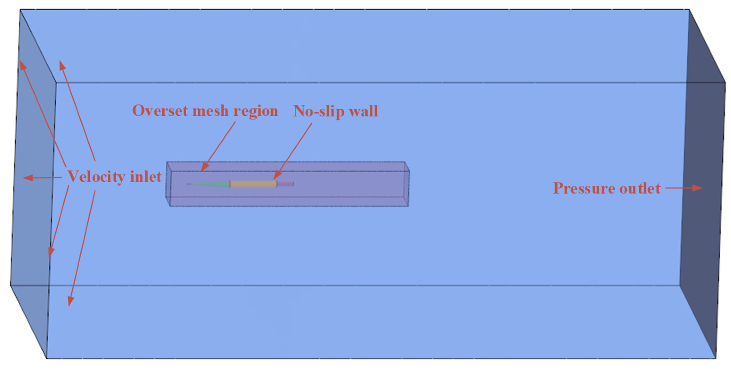
Based on the computational model, a rectangular background flow domain is constructed, together with an overset region for vehicle motion. The dimensions and boundary conditions of each domain are specified as follows, and a schematic of the computational domain and boundary conditions is shown in Figure 1.

(1)

Inlet: The inlet boundary is located at a distance of 1L from the nose end face of the vehicle, where L is the vehicle length. Its size is 10D × 10D, where D is the vehicle diameter. The four side faces surrounding the rectangular flow domain are also specified as velocity-inlet boundary conditions, with the inlet velocity set to 0.

(2)

Outlet: The outlet boundary is located at a distance of 4L from the tail end face of the vehicle, where L is the vehicle length. Its size is 10D × 10D, where D is the vehicle diameter. The outlet is specified as a pressure-outlet boundary with a pressure of 1.7 atm.

(3)

Overset mesh: The surface of the vehicle motion domain is defined as an overset-mesh boundary, which is combined with the outer flow domain of the vehicle to form the overset mesh interface.

(4)

Wall: The vehicle surface is specified as a no-slip wall boundary.

2.2. Grid Model

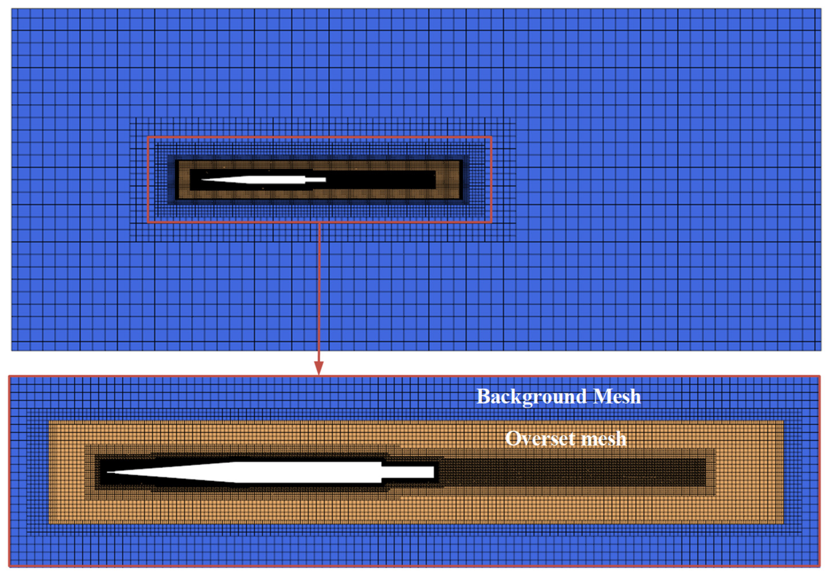
To simulate the acceleration motion of the underwater hypervelocity vehicle, the overset mesh technique is employed. This method avoids mesh distortion under large-amplitude vehicle movement, and separates motion and background domains for targeted local refinement around the vehicle and cavity interface. By means of hole cutting and interpolation, boundary information is exchanged among different mesh regions for flow-field computation, thereby establishing the coupling among different mesh regions and enabling the numerical solution of the entire computational domain. Trimmed hexahedral meshes are used to discretize the entire flow domain. Mesh refinement is applied near the vehicle surface to capture flow-field features in regions with large gradients. A wall-function approach is employed in the near-wall region, and prism-layer meshes are generated to resolve the viscous gradients near the wall. The height of the first layer mesh near the wall is adjusted to ensure y+ < 1 on walls, to match the wall-resolved requirement of turbulence model [25]. In the estimated cavity envelope region, local mesh refinement is further performed to achieve accurate resolution of the cavity interface. The meshes of the background and overset regions are coupled in real time through the overset mesh technique to form the overall computational mesh for numerical computation. Figure 2 shows the overall computational mesh and local mesh details.

2.3. Numerical Model

In this study, a numerical model for the multiphase flow during the acceleration of an underwater hypervelocity vehicle is established based on homogeneous equilibrium flow theory, a rigid-body motion model, and the overset mesh method. The finite volume method is adopted for spatial discretization. The IDDES model is employed to improve the prediction accuracy of unsteady supercavitating flows at high Reynolds numbers. The VOF multiphase flow model is used to describe the two-phase medium within a unified continuum, while the Schnerr–Sauer cavitation model is introduced to account for mass transfer between phases. The governing equations and mathematical models used in the numerical simulation are given as follows:

(1)

Governing equations

The governing equations consist of the continuity equation and the Navier–Stokes equation, which are written as follows:

$${\displaystyle \frac{\partial {\rho }_m}{\partial t}}+\nabla \cdot ({\rho }_{m}u)=0$$

$${\displaystyle \frac{\partial ({\rho }_{m}u)}{\partial t}}+\nabla \cdot ({\rho }_{m}uu)=-\nabla p+\nabla \cdot \tau +{\rho }_m\mathrm{g}$$

where ${\rho }_m$ is the mixture fluid density, $p$ is the pressure field, $u$ is the velocity vector of mixed fluid, and $\tau$ is the viscous stress tensor.

(2)

Volume fraction equation

Assuming that the phases are interpenetrating, the phase volume fraction is introduced accordingly. In this study, the homogeneous VOF multiphase flow model is adopted, in which the multiphase flow is treated as a single equivalent fluid medium [26]. Supercavitating flow is a typical application of high-resolution schemes in interfacial flow simulations [9]. Therefore, the High-Resolution Interface-Capturing (HRIC) scheme is employed to capture the gas–liquid interface [27], thereby avoiding inaccurate interface capturing caused by numerical diffusion. The density of the mixture phase in three-phases flow is expressed as follows:

$${\rho }_m={\rho }_g{\alpha }_g+{\rho }_v{\alpha }_v+{\rho }_l\left(1-{\alpha }_g-{\alpha }_v\right)$$

where $\alpha$ is the volume fraction; $\rho$ is the density; and the subscripts $m$, $v$, $g$, and $l$ denote the mixture phase, water vapor, air, and liquid water, respectively.

(3)

Turbulence model

The IDDES model [28] combines the advantages of the Reynolds-Averaged Navier–Stokes (RANS) and Large Eddy Simulation (LES) methods by reconstructing the subgrid-scale model in LES. Specifically, the RANS model is used in the near-wall region, while the LES model is applied in the remaining flow-field region to capture unsteady vortex, flow separation and re-entrant jet of supercavity. In this way, computational accuracy can be ensured while reducing the requirements on mesh quality. In the IDDES model, the $k$ equation and the $\omega$ equation are modified, which can be written as follows:

$${\displaystyle \frac{\partial }{\partial t}}\left(\rho k\right)+\nabla \cdot \left(\rho \overline{U}k\right)=\nabla \cdot \left[\left(\mu +{\displaystyle \frac{{\mu }_t}{{\sigma }_k}}\right)\nabla k\right]+ P_k-{\beta }^{\prime }\rho k\omega F_{IDDES}$$

$${\displaystyle \frac{\partial }{\partial t}}\left(\rho \omega \right)+\nabla \cdot \left(\rho \overline{U}\omega \right)=\nabla \cdot \left[\left(\mu +{\displaystyle \frac{{\mu }_t}{{\sigma }_{\omega }}}\right)\nabla \omega \right]+ (1-F_1)2\rho {\displaystyle \frac{\nabla k\nabla \omega }{{\sigma }_{\omega 2}\omega }}+\alpha {\displaystyle \frac{\omega }{k}}{P}_k-\beta \rho {\omega }^2$$

where $k$ is the turbulent kinetic energy, $\omega$ is the specific dissipation rate, $F_1$ is the blending function, $P_k$ is the result term, ${\sigma }_k$, ${\sigma }_{\omega }$, and ${\sigma }_{\omega 2}$ are model coefficients, $\alpha$ and $\beta$ are computational constants. Detailed values of the relevant parameters can be found in Ref. [29]. $F_{IDDES}$ is the shielding function used to determine whether the LES method or the RANS method is adopted, which is expressed as follows:

$$F_{IDDES}={\displaystyle \frac{l_{RANS}}{l_{IDDES}}}$$

$$l_{IDDES}={\tilde{f}}_d\cdot \left(1+f_e\right)\cdot l_{RANS}+\left(1-{\tilde{f}}_d\right)\cdot l_{LES}$$

$${\tilde{f}}_d=\max \left[\left(1-f_{dt}\right),f_B\right]$$

$$l_{RANS}={\displaystyle \frac{\sqrt{k}}{\beta \omega }}$$

$$l_{LES}=C_{DES}\Delta$$

$$\Delta =\min \left[0.15\max \left(d,{\Delta }_{\max }\right),{\Delta }_{\max }\right]$$

$${\Delta }_{\max }=({\Delta }_x,{\Delta }_y,{\Delta }_z)$$

where $l_{RANS}$, $l_{LES}$ and $l_{IDDES}$ are the turbulent length scales of RANS, LES and hybrid IDDES, respectively, ${\tilde{f}}_d$, $f_{dt}$ and $f_B$ are delay correction factors for wall boundary discrimination, $C_{DES}$ is the DES length-scale constant, $\Delta$ is the local characteristic mesh size, $d$ is the wall distance of each cell, and ${\Delta }_x$, ${\Delta }_y$, and ${\Delta }_z$ represent the mesh size in three coordinate directions, with ${\Delta }_{\max }$ being the maximum value among the three directional mesh sizes of a single cell.

(4)

Cavitation model

The Schnerr–Sauer cavitation model [30] is employed to describe the mass transfer between water vapor and liquid water. Compared with other transport-based cavitation models, this model is more suitable for simulating the unsteady cavitation process and has been widely applied in the computation of unsteady cavitating flows [31,32]. The governing equations can be written as follows:

$$\left\{\begin{array}{l}{R}_e={\displaystyle \frac{{\rho }_v{\rho }_l}{{\rho }_m}}{\displaystyle \frac{3{\alpha }_v\left(1-{\alpha }_v\right)}{R_B}}\sqrt{{\displaystyle \frac{2}{3}}{\displaystyle \frac{P_v-P}{{\rho }_l}}}\hspace{1em}\hspace{1em} P<P_v\\ R_c={\displaystyle \frac{{\rho }_v{\rho }_l}{{\rho }_m}}{\displaystyle \frac{3{\alpha }_v\left(1-{\alpha }_v\right)}{R_B}}\sqrt{{\displaystyle \frac{2}{3}}{\displaystyle \frac{P-P_v}{{\rho }_l}}}\hspace{1em}\hspace{1em} P>P_v\end{array}\right.$$

where $R_e$ and $R_c$ are the vapor generation rate and condensation rate, respectively, $R_B$ is the bubble radius, and $P_v$ is the saturated vapor pressure.

(5)

Motion model

To numerically simulate the acceleration process of an underwater hypervelocity vehicle, the DFBI model and the 6-DOF motion model are employed. These models enable the coupled solution of the fluid and rigid body and allow rigid-body motion to be simulated by calculating the hydrodynamic forces acting on the body. In addition, by using the background and overset meshes and defining the prescribed vehicle motion and overset boundary conditions, interpolation relationships are established at the overset mesh interface for data exchange, thereby enabling real-time motion and mesh updating of the overset region [33].

(6)

Solution algorithm

In the numerical simulation of the unsteady acceleration process of the underwater hypervelocity vehicle, the flow field is solved using a segregated flow solver based on the SIMPLE algorithm. Both the convective and diffusive terms of the governing equations are discretized using a second-order upwind scheme, and a second-order scheme is used for temporal discretization.

2.4. Validation of the Mesh

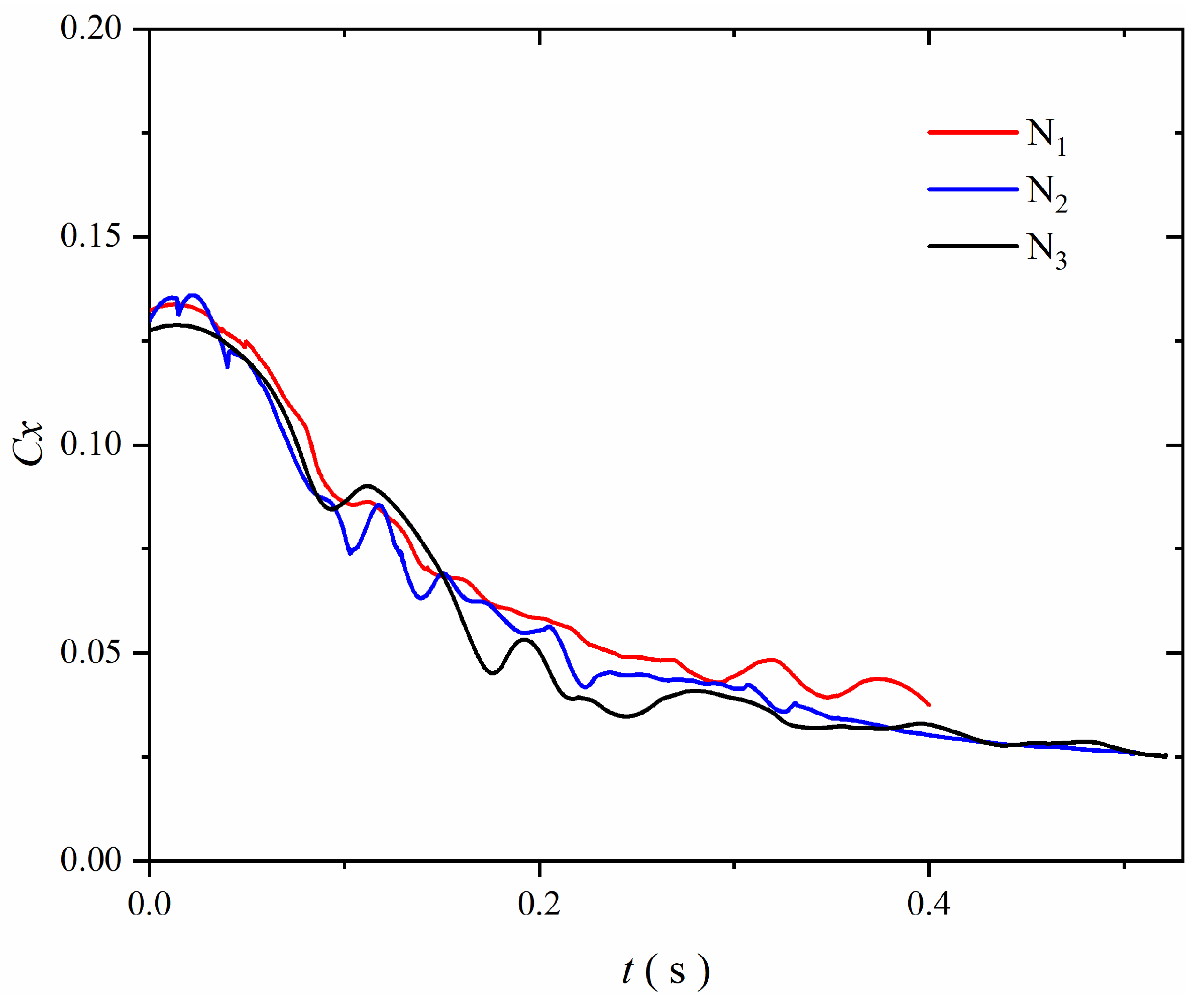
Grid-independence verification is an important prerequisite for ensuring the reliability and accuracy of numerical simulation results, especially for strongly nonlinear gas–liquid multiphase flow problems such as supercavitation. To eliminate the influence of mesh size on the numerical results of supercavitating flow and to ensure that the numerical simulations can faithfully reflect the actual flow behavior, three sets of computational meshes with different resolutions were designed in this study based on previous research experience. The corresponding mesh numbers were N₁ = 5.20 × 10⁶, N₂ = 1.11 × 10⁷, and N₃ = 1.58 × 10⁷. Using the instantaneous drag coefficient of the vehicle during acceleration as the evaluation criterion, it can be seen from Figure 3 that the variations in drag coefficient obtained with meshes N₂ and N₃ are generally consistent, and the drag-coefficient convergence error at the final instant is less than 0.5%. In addition, the grid convergence index (GCI) method proposed by Roache [34] was employed to assess mesh convergence. By considering parameters such as the mesh refinement ratio and grid convergence error, the calculated GCI value for mesh N₂ was 0.39%, which is lower than the threshold of 3% [35] and therefore satisfies the GCI criterion. This indicates that the numerical calculation has entered the asymptotic convergence region, and the dependence of the numerical solution on mesh size has been effectively controlled [36]. Considering both computational accuracy and computational cost, mesh N₂ was finally selected as the baseline mesh in this study.

2.5. Validation of the Time-Step

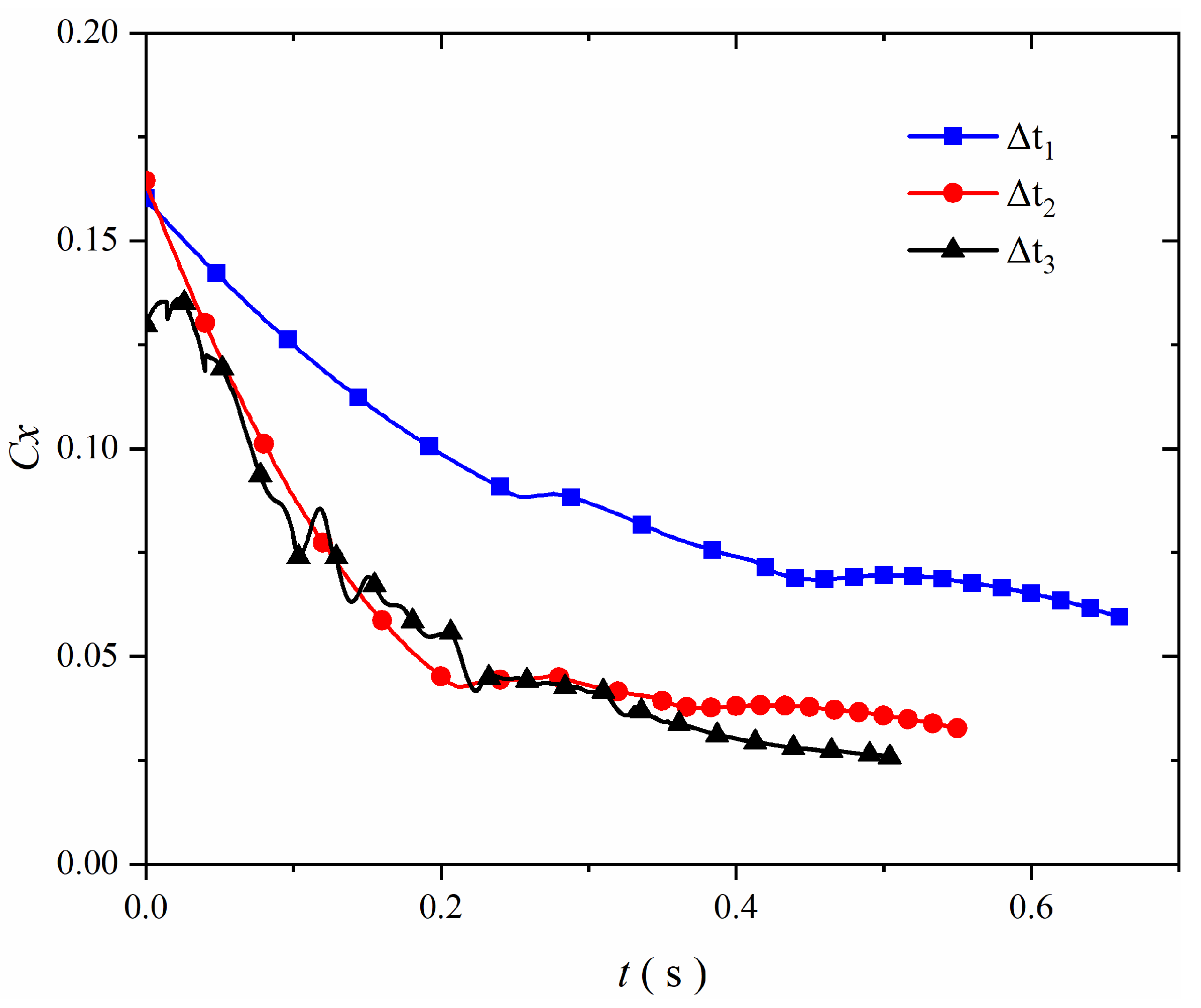
In the numerical simulation of unsteady supercavitating flow, the time-marching strategy directly affects the capturing accuracy of the multiphase interface and is therefore crucial for predicting the flow field and hydrodynamic characteristics during vehicle acceleration. Considering the mesh resolution and numerical stability requirements, and based on the baseline mesh validated by the grid-independence study, three time steps were selected, namely, Δt₁ = 1 × 10⁻³ s, Δt₂ = 1 × 10⁻⁴ s, and Δt₃ = 1 × 10⁻⁵ s. The time-varying drag coefficient during acceleration was used as the benchmark quantity. Figure 4 presents the drag coefficient histories of the vehicle obtained with different time steps. The results show that when the time step is equal to or smaller than Δt₂, the drag-coefficient variation tends to become consistent, indicating that the numerical results have basically reached time-step independence. However, Δt₃ provides a more detailed resolution of the drag-coefficient variation. Therefore, the final time step selected in this study is 1 × 10⁻⁵ s. Meanwhile, combined with the selected time step, grid size and flow velocity in the flow field, the Courant–Friedrichs–Lewy (CFL) number is calculated as 0.72, which is less than 1 and meets the numerical stability requirements for unsteady flow simulation [37].

2.6. Validation of Numerical Model

Ventilated supercavity water-tunnel experiments can accurately capture the unsteady morphological characteristics of ventilated supercavities, thus providing the most direct and reliable reference for validating numerical simulations. In the present study, an independently conducted ventilated supercavity water-tunnel experiment based on a scaled model of a supercavitating vehicle is used for validation. By systematically comparing the numerical results with the experimental measurements, the validity and accuracy of the adopted numerical method are verified.

The ventilated supercavity water-tunnel experiment was conducted under constant-speed and constant-pressure conditions. The cavity morphology during the formation and stable stages of the ventilated supercavity was obtained by external high-speed imaging. The experimental model consisted of three parts: a cavitator section, a support rod, and an L-shaped bracket. The cavitator section had a length of 46 mm and a diameter of 15 mm, while the support rod had a diameter of 25 mm and a length of 800 mm. The L-shaped bracket was used to stabilize the support rod. The model was mounted in a tail-support configuration and connected to the water-tunnel support strut through threads.

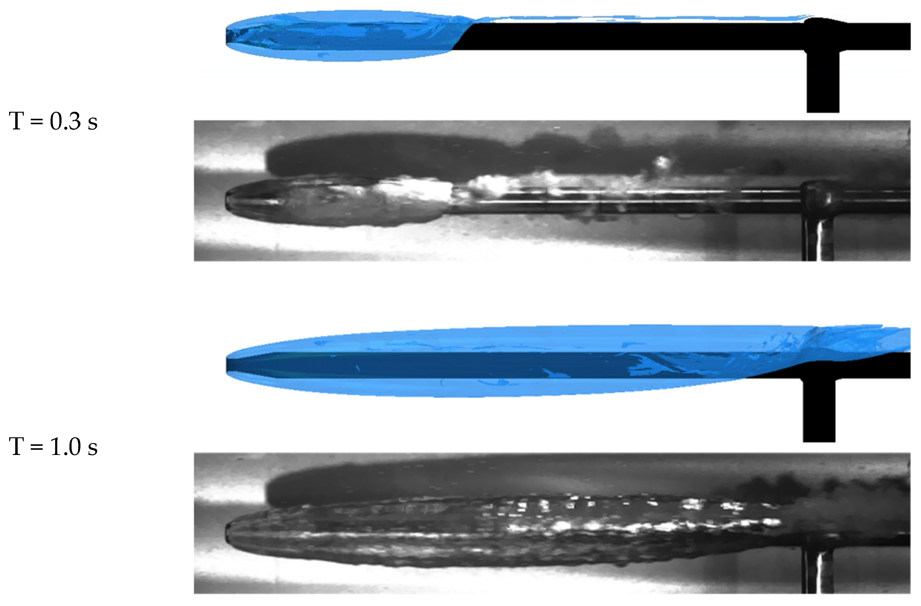
According to the water-tunnel test conditions and the experimental model setup, transient numerical simulations of ventilated supercavitation were carried out. The test velocity was 9 m/s. The experimental and numerical results at representative instants during the formation of the ventilated supercavity, corresponding to the local cavity and supercavity states, are shown in Figure 5. At specific instants during supercavity formation, qualitative comparison shows the cavity morphological features predicted by the numerical simulation, particularly the effects of gravity on the cavity shape, as well as the re-entrant jet and tail gas leakage, agree well with the water-tunnel experimental results. For a quantitative comparison of the cavity-core diameter and length, the average errors in diameter and length at the two selected instants are 7.6% and 5.2%, respectively, relative to the experimental results. Both qualitative and quantitative comparisons demonstrate that the numerical model established in this study can accurately predict the flow and morphological characteristics of supercavities under unsteady conditions.

2.7. Determination of the Ventilation Flow Rate

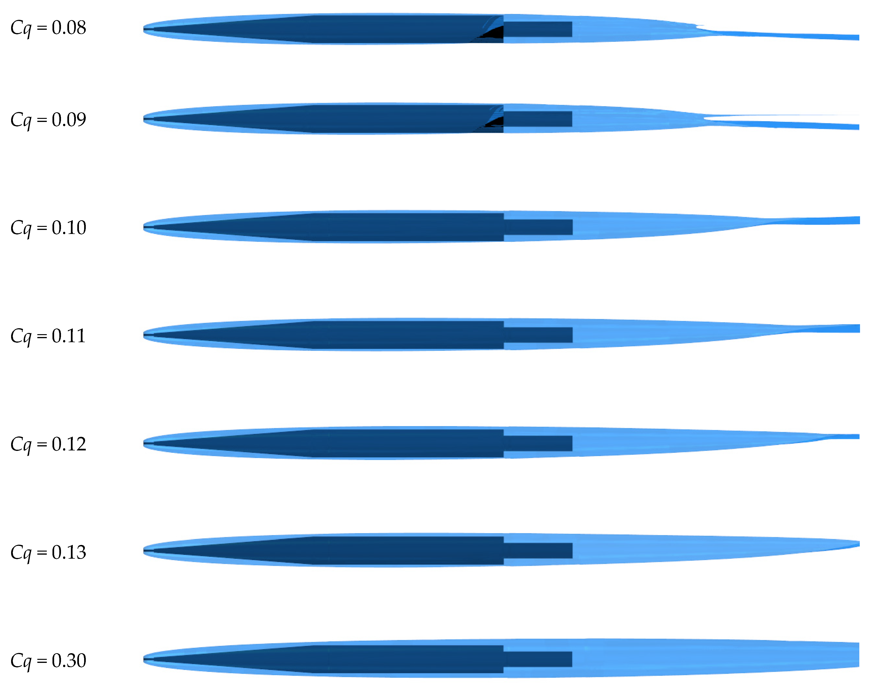
The underwater hypervelocity vehicle accelerates from its initial navigation state to the hypervelocity cruising state and experiences the stages of fully wetted flow, natural cavitation, ventilated cavitation, and ventilated supercavitation. To accelerate the formation of the ventilated supercavity and minimize the influence of the cavity formation process on vehicle stability, a strategy of supplying a relatively large amount of ventilation gas is adopted to accelerate supercavity formation [38]. To quickly determine the ventilation flow rate required during the acceleration process of the underwater hypervelocity vehicle, the ventilation demand for steady motion at 100 m/s was first calculated, and then three times the cruising-stage ventilation flow rate was used for the acceleration stage [38]. As shown in Figure 6, which presents the cavity morphology and size of the underwater hypervelocity vehicle under different ventilation flow rates, when the ventilation coefficient C_q is in the range of 0.08–0.10, the cavity diameter and length increase significantly with increasing ventilation coefficient, and a certain degree of wetted region remains near the vehicle tail at C_q = 0.8 and 0.09. When the ventilation coefficient is in the range of 0.10–0.13, the variations in cavity diameter and length are no longer significant, which is consistent with the findings of Skidmore [38]. Moreover, when the ventilation coefficient is 0.10, a supercavity that fully envelops the vehicle can be formed. Under small angles of attack, this condition is likely to generate a planing force associated with tail wetting, thereby satisfying the force-balance requirement of the vehicle. Therefore, the ventilation coefficient in the cruising stage is selected as 0.1, and the corresponding cavitation number is 0.0185, while that in the wide-speed-range acceleration stage is set to 0.3. Figure 6 also presents the cavity morphology at a ventilation coefficient of 0.3. In this case, the vehicle is basically located within the expanding section of the supercavity, which is expected to enable rapid supercavity coverage during vehicle acceleration.

3. Results and Discussion

Numerical simulations are performed to investigate the acceleration process of the underwater hypervelocity vehicle, with the initial conditions set as a vehicle speed of 70 m/s and a ventilation coefficient of 0.3, which are set as the benchmark conditions in this study.

3.1. Evolution of the Natural Cavity

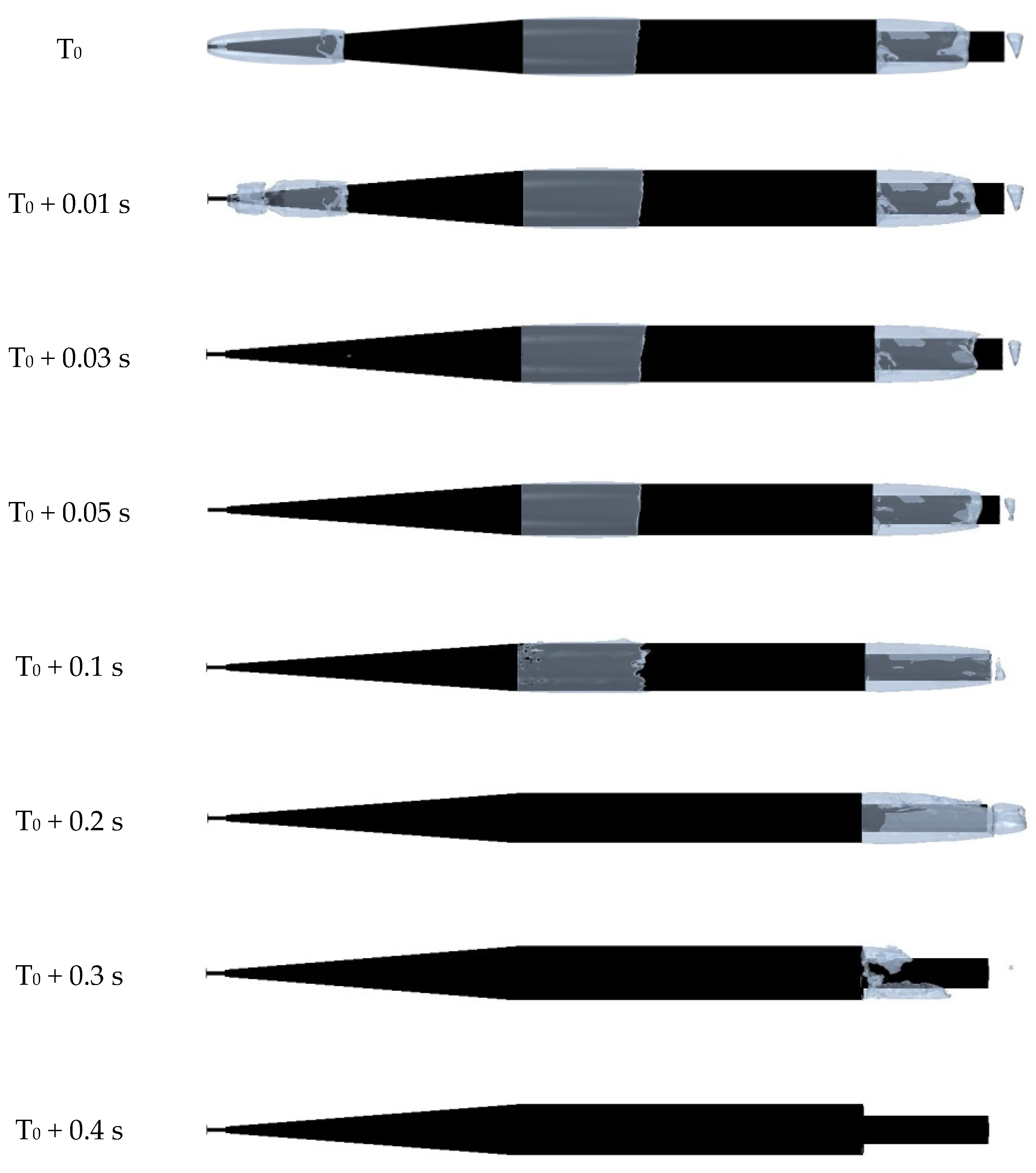
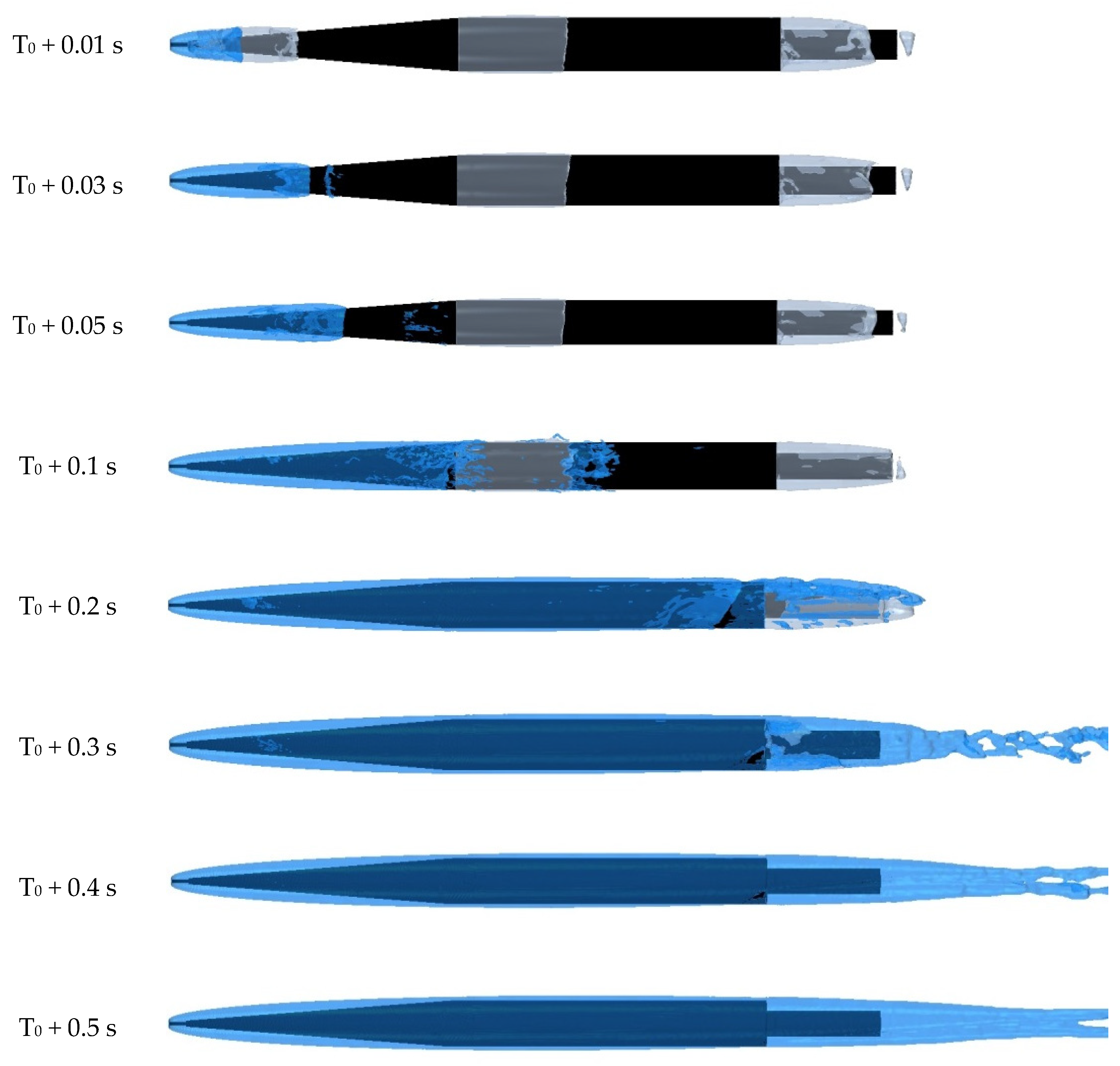
The evolution of the natural cavity during the acceleration of the underwater hypervelocity vehicle is shown in Figure 7. Under the initial-speed condition, the natural cavitation number is approximately 0.06, and the vehicle exhibits a three-cavity pattern, that is, obvious cavitation occurs at the bow, mid-body, and stern. The cavity lengths are approximately 2.5, 2.0, and 1.5 times the vehicle diameter, respectively. This cavitation mainly results from the relatively high initial vehicle speed and the correspondingly low natural cavitation number under shallow-water conditions. In addition, the cavitator at the bow, the conical section at the mid-body, and the stepped configuration at the stern jointly contribute to the pronounced natural cavitation behavior. After T₀, with the generation of the ventilated cavity, the evolution of natural cavitation intensifies. As shown in Figure 7 and Figure 8, at T₀ + 0.1 s, the integrity of the natural cavity is disrupted. At the ventilation location immediately behind the cavitator, the ventilated cavity first forms and occupies the original natural-cavity region. At this stage, the natural cavity and the ventilated cavity coexist, but the natural cavity is significantly compressed and deformed. Discontinuous “cavity rings” appear between the natural cavities at the beginning of the conical section, whereas the natural cavities in the region downstream of the cone and the long tail-tube region remain almost unchanged. As time proceeds, the ventilated cavity further develops, and the natural cavitation at the bow disappears completely. Subsequently, the natural cavitation region behind the cone also gradually vanishes. In the tail-tube region, the cavity size increases slightly because of the increasing velocity, indicating a slight enhancement of cavitation. During the period from T₀ + 0.2 s to T₀ + 0.4 s, the natural cavity at the stern coexists with the ventilated cavity. Eventually, the natural cavitation disappears progressively from back to front, and the cavity tail undergoes pronounced twisting and deformation. In the final state, the natural cavitation has basically disappeared. According to the calculated cavity morphology and the above analysis, a period of gas–vapor–liquid three-phase coexistence exists during the vehicle acceleration process. However, with the gradual formation of the ventilated supercavity, the ventilated cavity begins to play a dominant role. The final cavity morphology is that of a ventilated supercavity enveloping the entire vehicle, and the natural cavitation is basically suppressed.

3.2. Evolution of the Ventilated Cavity

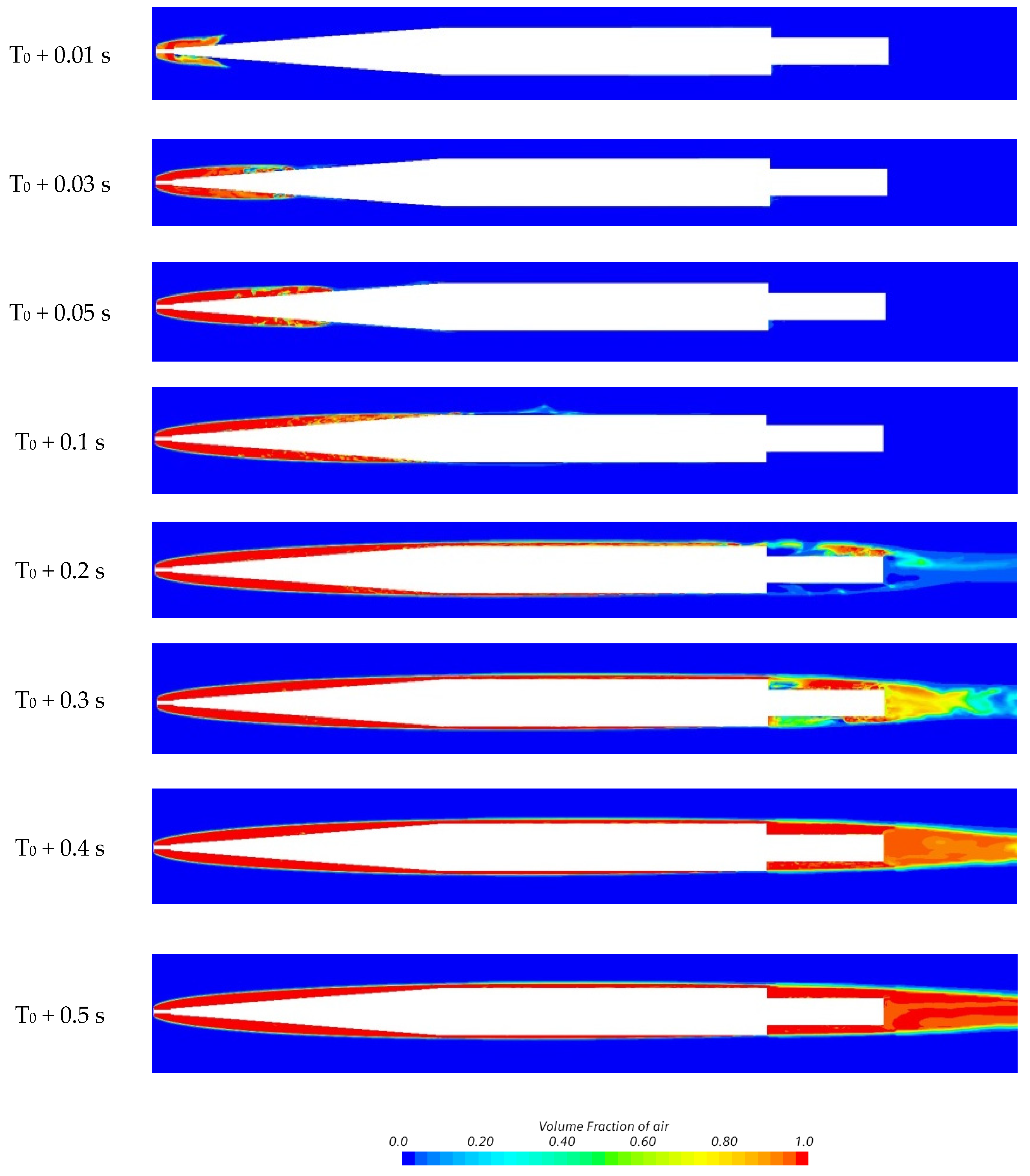
The cavity development during the acceleration of the underwater hypervelocity vehicle is shown in Figure 8 and Figure 9. In terms of the supercavity formation process, at 0.1 s, the ventilated cavity has passed over the conical section of the vehicle; at 0.2 s, it has reached the tail-tube region; at 0.3 s, a supercavity that nearly envelops the entire vehicle has formed; and at 0.5 s, the vehicle is fully enveloped by the gas phase. The numerical results indicate that the flow in the head and tail regions of the ventilated supercavity is relatively complex. In the head region, owing to the presence of the natural cavity, the initial ventilated cavity exhibits an open trumpet-like shape, with complex gas–vapor–liquid mixing and a pronounced re-entrant jet. After passing through the natural-cavity region, the ventilated cavity begins to close along the wall of the conical section. At the junction between the conical and cylindrical sections of the vehicle, the integrity of the ventilated cavity is disrupted due to the geometric transition of the vehicle and the presence of the natural cavity, and the gas phase is distributed in the regions before and after the natural cavity without forming a complete and continuous interface. When the cavity develops to the vicinity of the long tail tube, the multiphase mixing becomes more complex. The growth of the ventilated cavity is more strongly affected by the gas flow and gravity, causing it to float above the natural cavity, while gas is discharged backward from the tail in the form of local cavity structures. After the ventilated cavity is fully developed, the supercavity releases gas in the form of twin vortex tubes and reaches a stable ventilated supercavity configuration.

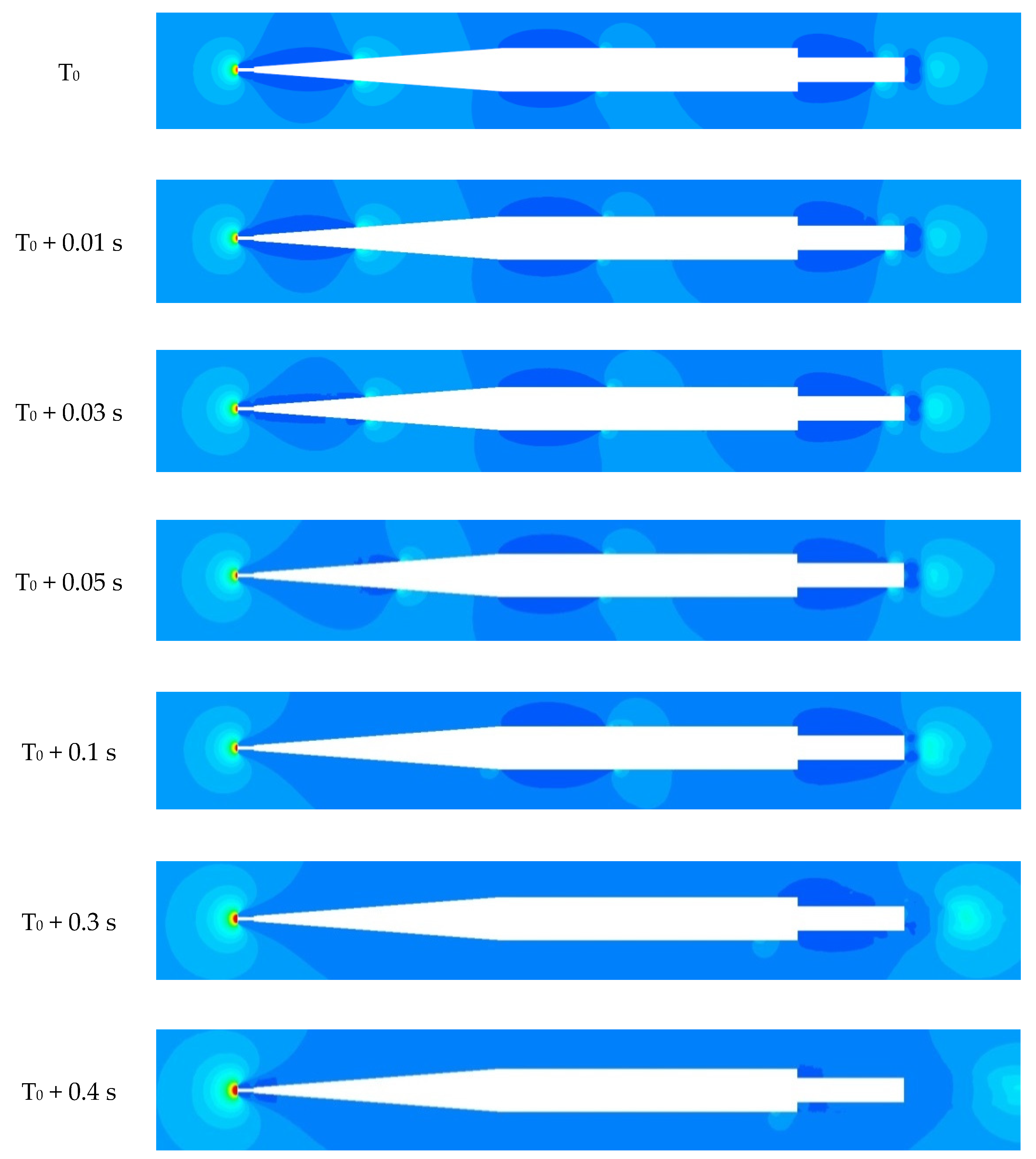
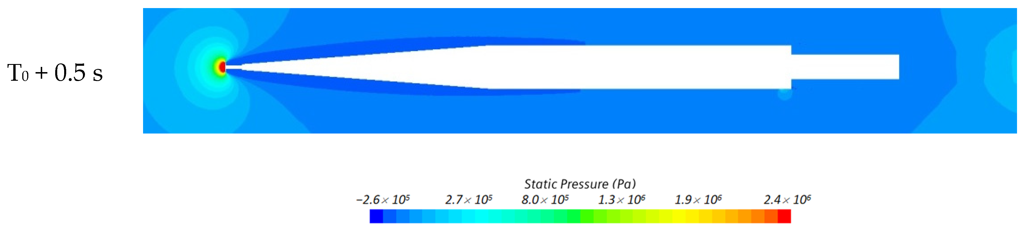
The evolution of the pressure field during the acceleration of the underwater hypervelocity vehicle is shown in Figure 10. The pressure contours also reflect the evolution of the cavity. A high-pressure region exists near the stagnation point on the upstream face of the cavitator at the head of the vehicle, and the area of this region gradually increases with increasing vehicle speed. At the initial moment, low-pressure regions of finite extent are present at the front, middle, and rear parts of the vehicle, while the pressure increases at the cavity closure locations, which correspond to the cavity locations. As time progresses and the cavity gradually envelops the vehicle, the low-pressure region surrounding the vehicle and the high-pressure region associated with cavity closure continuously move downstream, until the latter is located behind the vehicle.

3.3. Variation in the Drag Coefficient

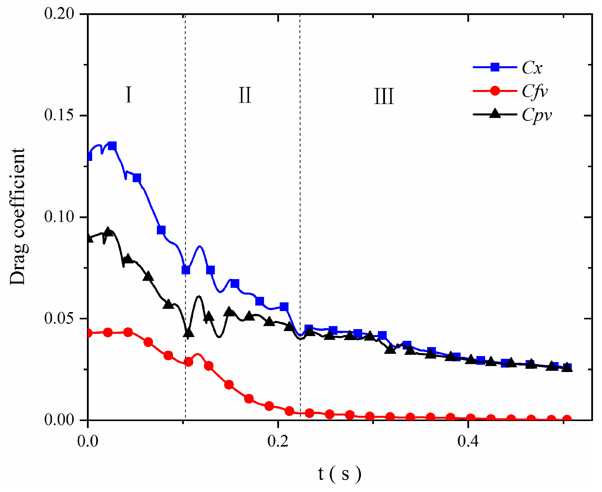
The time histories of the drag coefficients during the acceleration of the underwater hypervelocity vehicle are shown in Figure 11. The results indicate that, with the acceleration and ventilation processes, the total drag coefficient of the vehicle generally decreases and can be divided into three stages, namely Stages I, II, and III. Stage I occurs before approximately 0.1 s. At the initial stage of ventilated cavity generation, the ventilated cavity and the natural cavity interact with each other near the bow, leading to a slight increase in the drag coefficient. Subsequently, as the ventilated cavity continues to grow, the drag coefficient of the vehicle shows a clear decreasing trend. Stage II corresponds to the period when the ventilated supercavity passes over the mid-body conical section and the cylindrical section of the vehicle. During this stage, the cavity gradually begins to envelop the entire cylindrical section as time progresses. Stage III corresponds to the period when the ventilated supercavity has basically enveloped the entire vehicle. At this stage, the flow near the vehicle tail is complex, and the drag coefficient increases slightly, which is likely related to the coverage of the tail by the ventilated supercavity and the collapse of the natural cavity. With the increase in velocity and the continuous injection of gas, the drag coefficient continues to decrease, but at a slower rate, mainly because the cavity has already enveloped the entire vehicle, and the drag coefficient has been reduced to a relatively low level. From the cavity evolution history shown in Figure 9 and the drag-coefficient history shown in Figure 11, it can be seen that complete cavity coverage and a substantial reduction in the drag coefficient can be achieved within a relatively short acceleration time. In terms of the drag components, during Stage I, when the supercavity is forming, the pressure drag coefficient and friction drag coefficient are comparable. During Stage II, as the supercavity continuously envelops the cylindrical section of the vehicle, the friction drag coefficient gradually decreases, and after 0.2 s, it is nearly reduced to zero. This can be clearly seen from the cavity coverage state in the cavity evolution history shown in Figure 9. At this stage, pressure drag becomes the dominant drag component, which is consistent with the drag-reduction mechanism of supercavitating vehicles.

3.4. Variation in the Motion Parameters

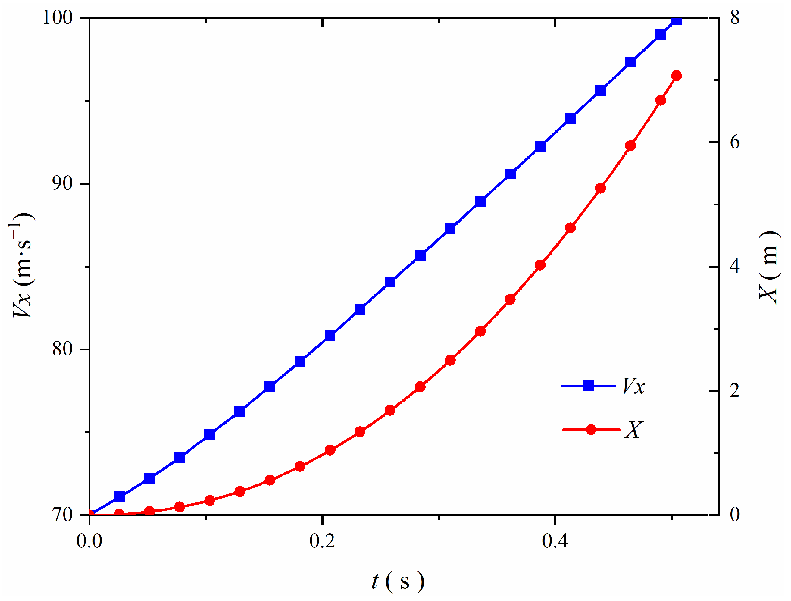
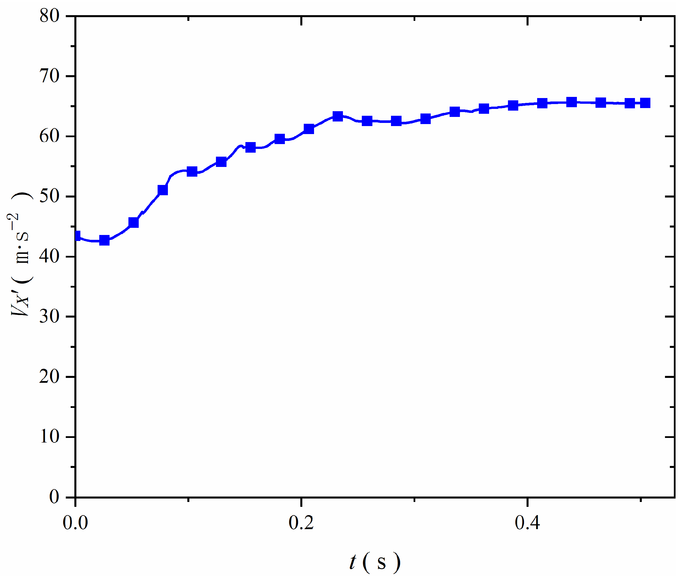
The time histories of the vehicle velocity and displacement during the acceleration process are shown in Figure 12. Overall, the variations in velocity and displacement are relatively smooth. The velocity varies approximately linearly with time. As indicated by the rate of change in velocity in Figure 13, the rate of increase in velocity gradually rises before 0.2 s and then remains nearly constant. This behavior is related to the cavity coverage over the vehicle surface. As can be seen from the time histories of the ventilated cavity in Figure 8 and Figure 9, after 0.2 s, the supercavity has basically enveloped the entire vehicle. At this stage, the vehicle moves approximately with uniform acceleration, accelerating from 70 m/s to 100 m/s within 0.5 s. The displacement varies approximately quadratically with time. As the velocity increases, the displacement increases more rapidly in the second half of the acceleration process. Owing to the short acceleration duration, the overall travel distance is also limited, with a total displacement of about 7 m. The short duration and limited displacement of the ventilated acceleration process enable the underwater hypervelocity vehicle to transition rapidly from the unsteady ventilated acceleration stage to the cruising stage, thereby contributing to the motion stability of the vehicle during the ventilated acceleration process.

3.5. Effect of the Ventilated Timing

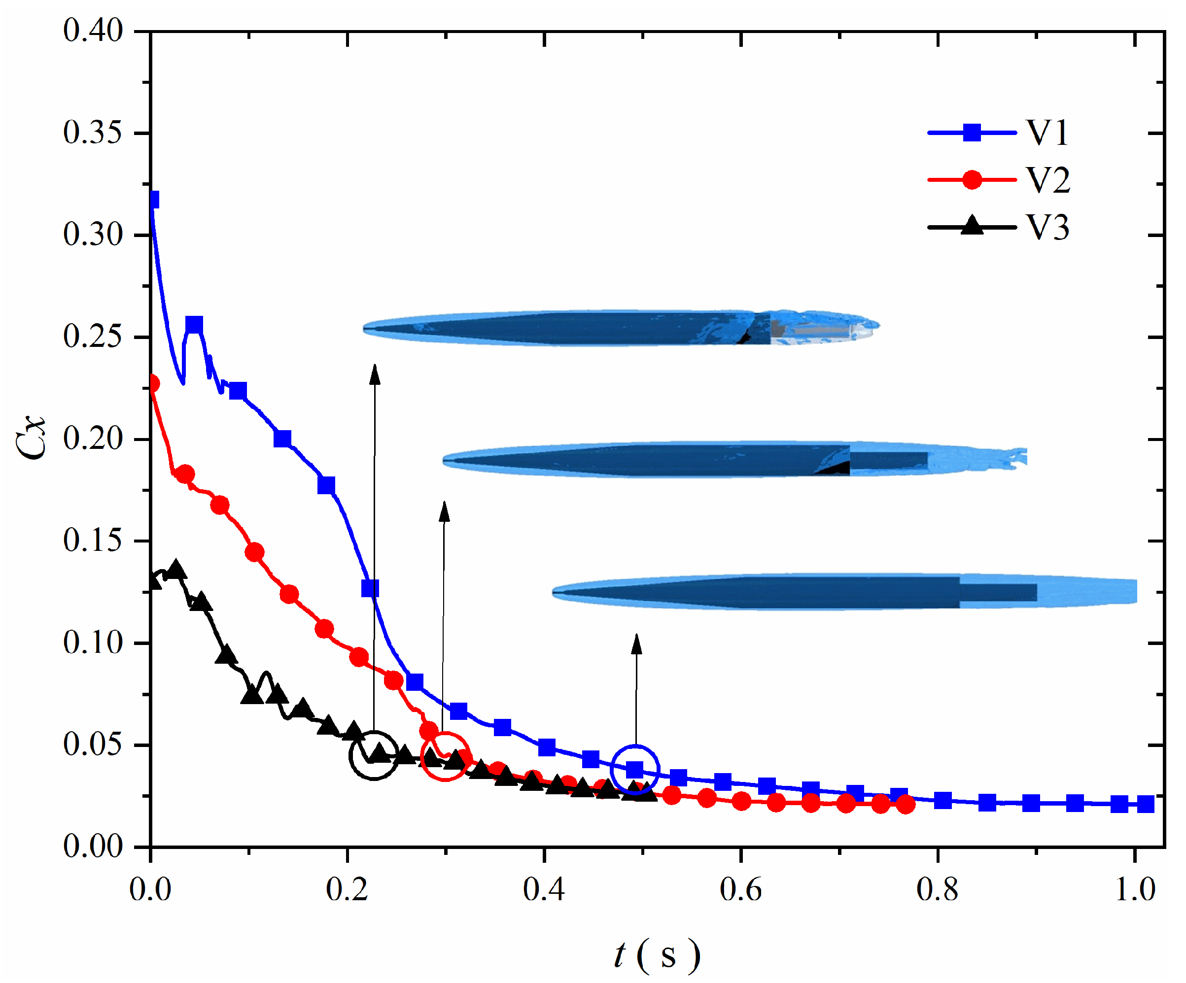
To analyze the effect of ventilation timing during vehicle acceleration, namely, the influence of ventilation initiated at different vehicle speeds on the multiphase flow, especially on the formation and enclosure of the supercavity, three ventilation conditions corresponding to vehicle speeds of 30, 50, and 70 m/s are considered, denoted as States V1, V2, and V3, respectively. The corresponding variations in the total drag coefficient are shown in Figure 14. Compared with State V3, at the initial moment of ventilation in States V1 and V2, the vehicle speed is lower and natural cavitation is still weak, resulting in significantly larger drag coefficients. Under ventilation, the drag coefficient in all three cases gradually decreases. Consistent with the evolution of the ventilated cavity described in Section 3.2, the drag-coefficient variation mainly exhibits a three-stage pattern, namely, the cavity gradually passes over the conical section, then over the cylindrical section, and finally enters the supercavity formation stage.

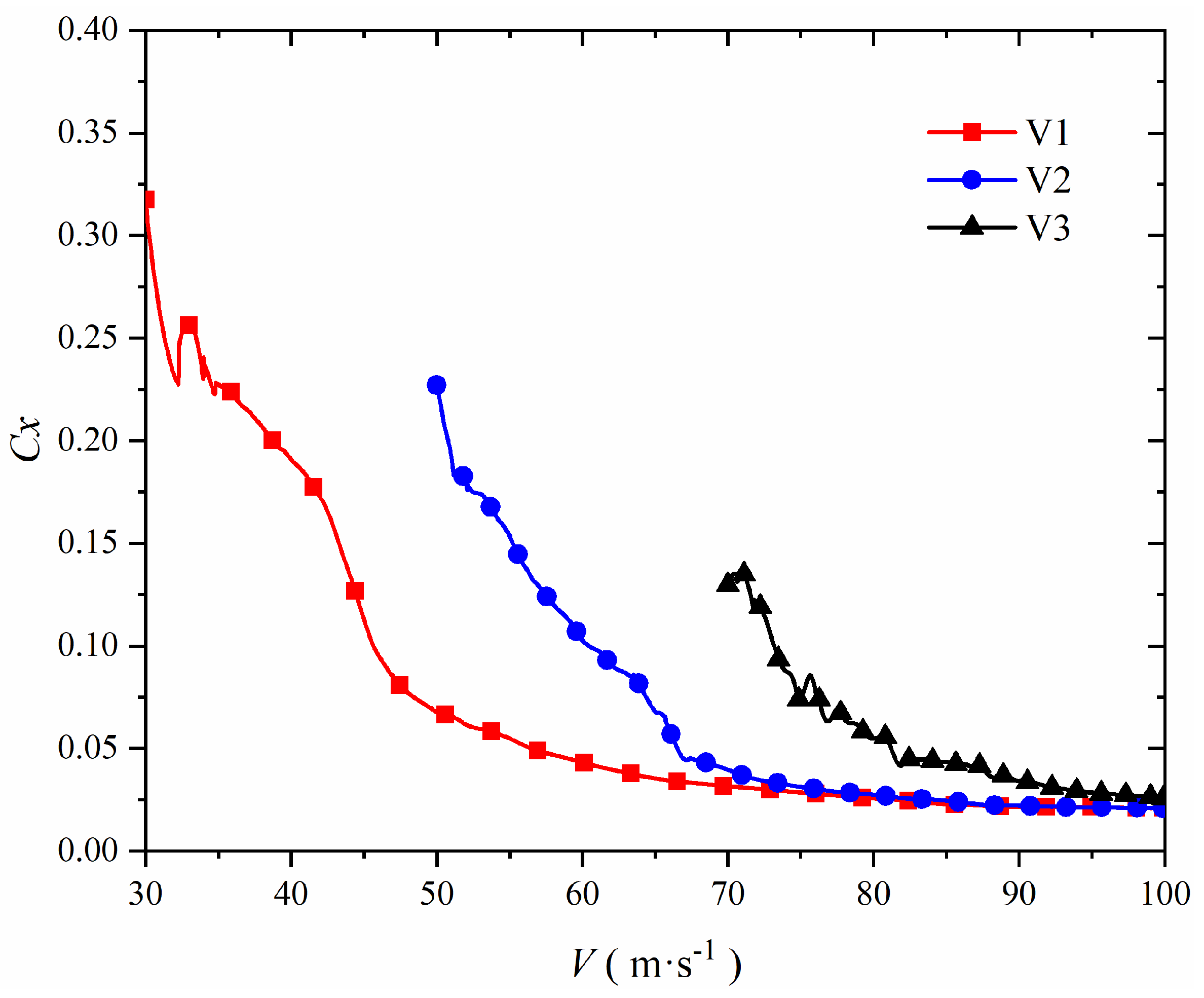
The three arrows shown in Figure 14 mark the characteristic instants at which the supercavity basically envelops the vehicle under the three speed conditions, along with the corresponding cavity morphologies. In these instances, the elapsed times from the onset of ventilation are approximately 0.2 s, 0.3 s, and 0.5 s, respectively. In State V3, at this characteristic instant, the cavity is mainly a ventilated supercavity, while the stern region remains in a mixed state of natural and ventilated cavities, and the overall flow is relatively complex. In State V2, a typical tail-planing closure state has already formed at this characteristic instant. In State V1, the ventilated supercavity has fully enveloped the entire vehicle at this characteristic instant, and the cavity interface is intact and smooth. However, due to the low vehicle speed at the initial ventilation moment, a relatively long unstable period exists during cavity formation, during which gas–liquid multiphase coexistence persists. In contrast, the time required for supercavity formation and vehicle acceleration can be significantly reduced in States V2 and V3. Physically, low-speed ventilation suffers high initial viscous drag from weak natural cavitation, and sustained mild three-phase mixing delays drag reduction. For high-speed ventilation, early natural and ventilated cavities rapidly evolve into full supercavity with rising velocity, greatly lowering the drag coefficient. To further compare the effects of ventilation at different speeds, Figure 15 presents the variation in the vehicle drag coefficient with velocity. Its overall trend is consistent with that shown in Figure 14, with the main difference being that ventilation initiated at a lower speed can reduce the vehicle drag coefficient earlier.

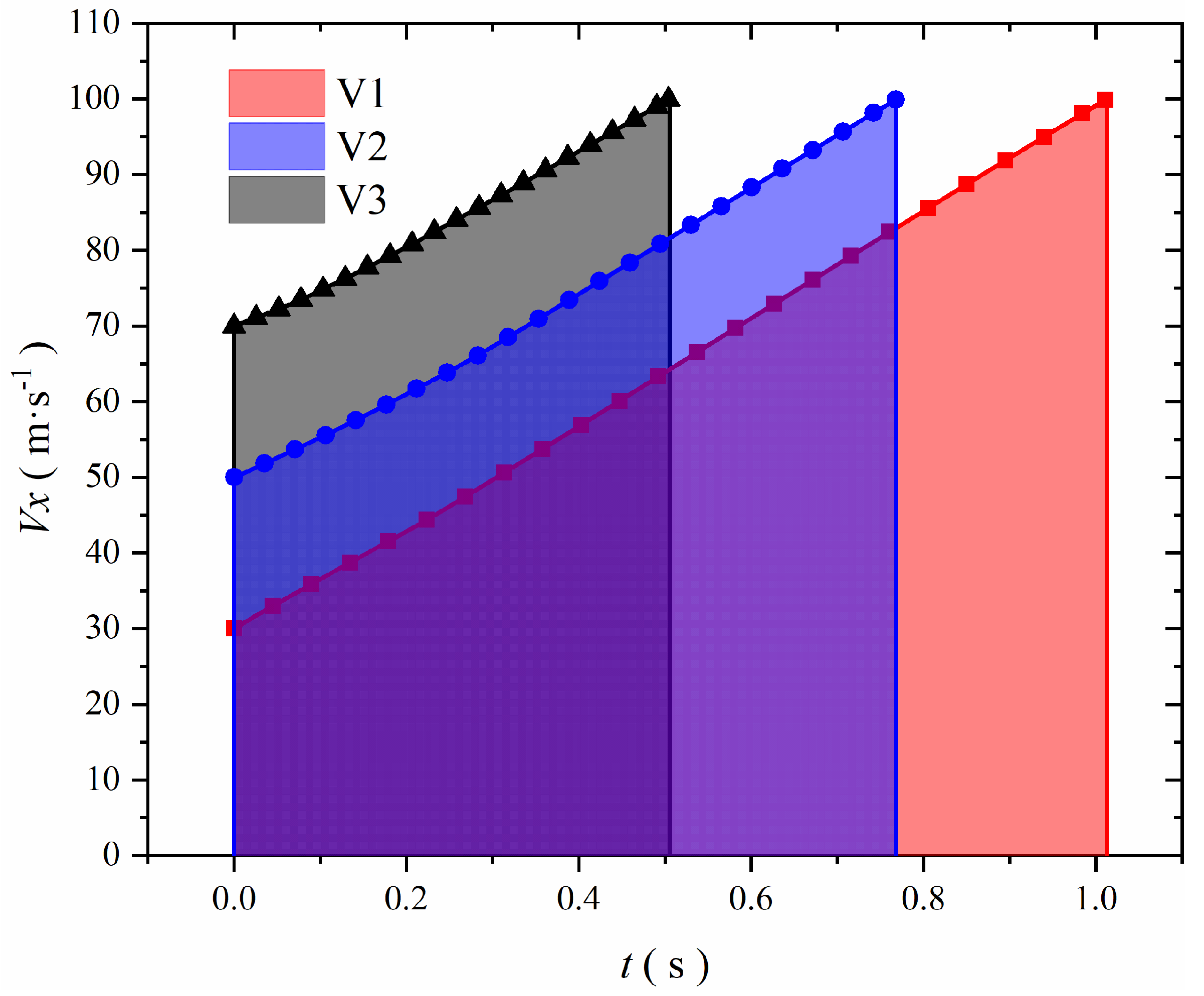
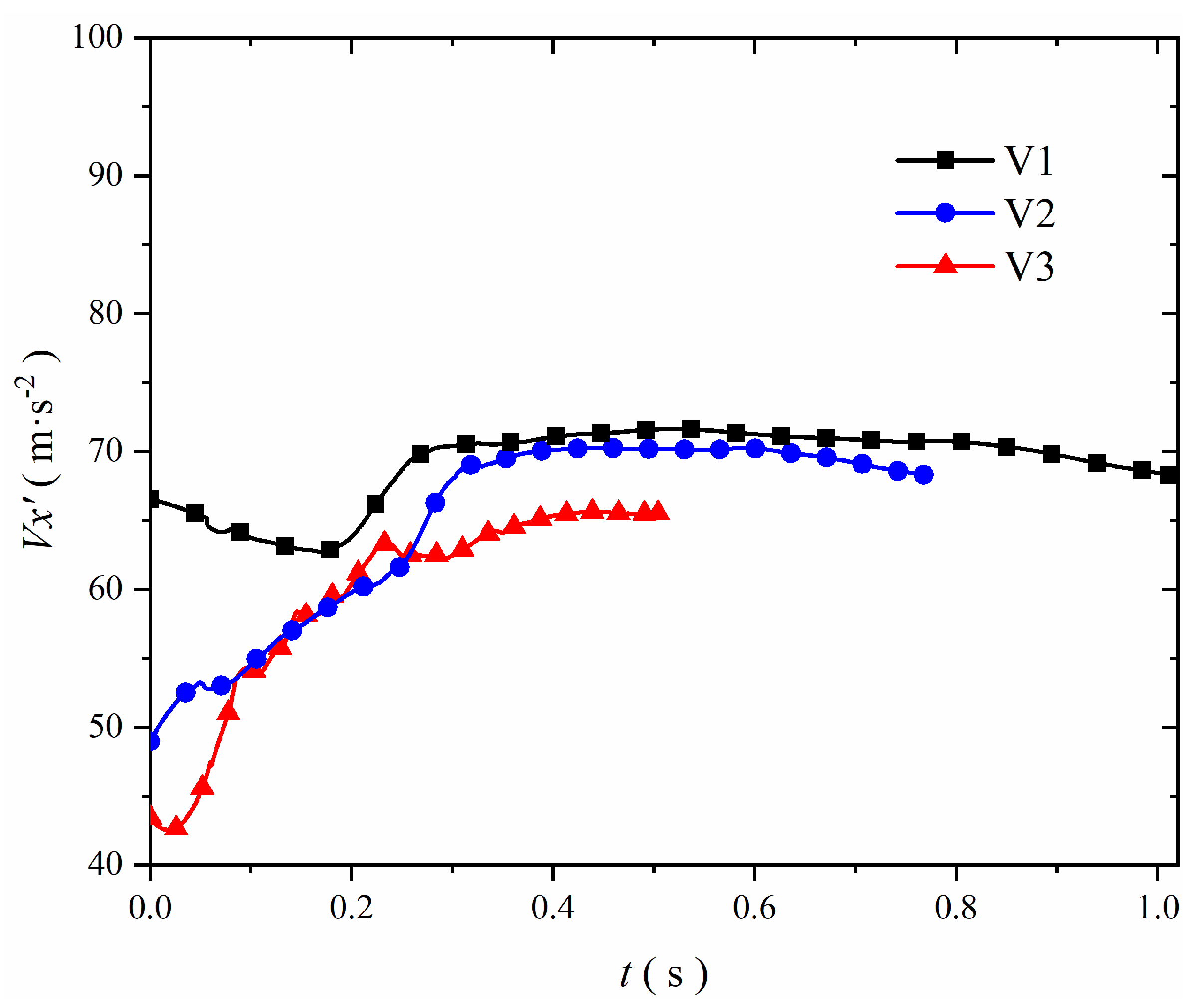
Figure 16 shows the velocity and displacement histories of the vehicle under different ventilation timings, in which the curves represent the velocity variation, and the shaded areas represent the displacement variation. Under ventilation initiated at the three vehicle speeds, the variations in vehicle velocity and displacement are generally similar. The displacement is more sensitive to ventilation at different vehicle speeds, and the displacement under the three speed conditions increases approximately in a proportional manner, which may introduce instability during navigation. Overall, the velocity varies approximately linearly. To further analyze the influence of different conditions on the velocity, Figure 17 presents the time histories of the vehicle acceleration under ventilation at different vehicle speeds. Overall, the accelerations are all positive under the three conditions, indicating that the vehicle remains in an accelerating state in all cases. When ventilation is applied in State V1, the acceleration first decreases, then increases, and finally becomes nearly constant. This corresponds to the initial ventilation stage, in which vapor–gas–liquid mixing occurs and local wetting appears on the vehicle surface, resulting in a slight increase in drag. With the gradual development of the cavity and the complete enclosure of the vehicle within the supercavity, the acceleration begins to stabilize. When ventilation is applied in States V2 and V3, the acceleration gradually increases and then becomes stable, showing a clear difference from the trend in State V1. The main reason is that, before ventilation, the latter two conditions are associated with larger drag, and therefore their initial acceleration values are smaller. By comparison, State V3 exhibits a larger acceleration, corresponding to faster supercavity formation. Therefore, a higher initial vehicle speed is beneficial to rapid supercavity formation and faster vehicle acceleration.

4. Conclusions

A coupled numerical model integrating multiphase flow, cavitation, turbulence, and six-degree-of-freedom motion was established in this study. After validation in terms of mesh resolution, time step, and model accuracy, the model was shown to accurately predict the cavity morphology, hydrodynamic characteristics, and motion behavior of an underwater hypervelocity vehicle during acceleration. It is therefore suitable for solving coupled problems involving gas–vapor–liquid multiphase flow and vehicle dynamics. Based on this established model, numerical simulations were performed to investigate the multiphase flow and motion characteristics of the underwater hypervelocity vehicle during acceleration. The main conclusions are as follows:

(1)

The ventilated cavity exerts a pronounced squeezing and suppressing effect on the natural cavity. At the initial stage of ventilation, the natural cavities form a three-cavity pattern at the bow, mid-body, and stern of the vehicle. As the ventilated cavity expands, the natural cavities are gradually squeezed, split, and eventually disappear, resulting in a supercavity dominated by the ventilated cavity. During this process, the evolution of the cavity interface exhibits pronounced unsteady characteristics.

(2)

The evolution of the vehicle drag coefficient exhibits a three-stage pattern. In the first stage, the ventilated cavity and the natural cavity interact with each other, and the drag coefficient rises slightly before decreasing. In the second stage, the cavity gradually envelops the cylindrical section of the vehicle, and the friction drag decreases significantly. In the third stage, the supercavity is formed; the friction drag approaches zero, and the pressure drag becomes dominant, while the total drag coefficient decreases to below 0.1, indicating a significant drag-reduction effect.

(3)

Ventilation timing has a significant effect on the formation time and flow stability of the supercavity. A comparison of ventilation at different vehicle speeds shows that low-speed ventilation can reduce drag earlier, but it results in a longer multiphase coexistence period and a longer cavity formation process, whereas high-speed ventilation can form a stable supercavity more rapidly. For ventilation initiated at initial speeds of 70 m/s, 50 m/s and 30 m/s, the time required for the supercavity to fully wrap the vehicle is approximately 0.2 s, 0.3 s, and 0.5 s, respectively. Ventilation at an initial speed of 70 m/s shortens the full supercavity formation time by more than 50% relative to ventilation at 30 m/s. Under the three ventilation conditions, the velocity increases approximately linearly, while the displacement varies approximately quadratically. When ventilation is initiated at a higher vehicle speed, the acceleration process is shorter, and the transition to the cruising state is faster, which is beneficial for improving navigation stability.

References

1. Ceccio, S.L. Friction Drag Reduction of External Flows with Bubble and Gas Injection. Annu. Rev. Fluid Mech. 2011, 42, 183–203. [Google Scholar]
2. Huang, Z.G.; Xiang, M.; Zhang, S.Q.; Xu, Z.H.; Wang, X.C. Analysis on coupling characteristics of ventilated cavitation and supersonic exhaust jet of a supercavitating vehicle. Appl. Ocean Res. 2026, 170, 105013. [Google Scholar] [CrossRef] [Scilit]
3. Cao, W.; Wei, Y.; Wang, C.; Zou, Z.; Huang, W. Current status, problems and applications of supercavitation technology. Adv. Mech. 2006, 36, 571–579. [Google Scholar]
4. Kuklinski, R.; Castano, J.; Henoch, C. Experimental study of ventilated cavities on dynamic test model. In Proceedings of the 4th International Symposium on Cavitation, Pasadena, CA, USA, 20–23 June 2001. [Google Scholar]
5. Li, J.; Wang, C.; Yan, W.; Bao, J.; Li, W.; Ding, Y.; Yang, Q.; Liu, Y. Study on drag reduction and lift characteristics of ventilated supercavitating vehicle under the synergistic effect of multiple parameters. Phys. Fluids 2025, 37, 093355. [Google Scholar] [CrossRef] [Scilit]
6. Li, S.L.; Xie, Z.; Li, S.B.; Huang, W.; Liu, S.; An, K. Investigation on drag reduction mechanism of trans-media vehicle with spike in high-speed underwater motion. Appl. Ocean Res. 2025, 165, 104833. [Google Scholar]
7. Kumar, G.; Nagothu, V.; Aman, R.; Karn, A. Supercavity Enhancement in High-Speed Heavyweight Torpedoes: Exploring the Role of Secondary Cavitator. J. Mar. Sci. Appl. 2026, 25, 423–432. [Google Scholar]
8. Pham, V.D.; Ahn, B.K. Numerical study of sweep angle effects of the control fin in supercavitating flow. Eng. Appl. Comput. Fluid Mech. 2025, 19, 2459669. [Google Scholar] [CrossRef] [Scilit]
9. Kinzel, M.P.; Krane, M.H.; Kirschner, I.N. A numerical assessment of the interaction of a supercavitating flow with a gas jet. Ocean Eng. 2017, 136, 304–313. [Google Scholar] [CrossRef] [Scilit]
10. Lindau, J.W.; Kuntz, R.F.; Merkle, C.L. Fully coupled 6-DOF to URANS, Modeling of cavitating flows around a supercavitating vehicle. In Proceedings of the Fifth International Symposium on Cavitation, Osaka, Japan, 1–4 November 2003. [Google Scholar]
11. Choe, Y.; Kim, C. Computational investigation on ventilated supercavitating flows and its hydrodynamic characteristics around a high-speed underwater vehicle. Ocean Eng. 2022, 249, 110865. [Google Scholar] [CrossRef] [Scilit]
12. Xu, H.Y.; Wang, C.; Wei, Y.; Cao, W. On the nonlinear hydrodynamic characteristic of a ventilated supercavitating vehicle with high Froude number. Ocean Eng. 2023, 268, 113457. [Google Scholar] [CrossRef] [Scilit]
13. Xu, H.Y.; Wang, C.; Wei, Y.; Wang, W.; Chang, S.; Han, Y. Numerical investigation of unsteady shedding behaviors of a reentrant jet supercavity. Phys. Fluids 2024, 36, 067125. [Google Scholar] [CrossRef] [Scilit]
14. Erfanian, M.R.; Moltani, A.A.; Mahmood, P.F. Parametric hydrodynamic analysis of ventilated supercavity dynamics under free-surface interaction: Combined effects of submergence depth, Froude number, and air entrainment. Eur. J. Mech./B Fluids 2026, 118, 204485. [Google Scholar] [CrossRef] [Scilit]
15. Savchenko, Y.N. Supercavitation Problems and Perspectives. In Proceedings of the 4th International Symposium on Cavitation, Pasadena, CA, USA, 20–23 June 2001. [Google Scholar]
16. Rand, R.; Pratap, R.; Ramani, D.; Cipolla, J.; Kirschner, I. Impact dynamics of a supercavitating underwater projectile. In Proceedings of the ASME Design Engineering Technical Conferences, Sacramento, CA, USA, 14–17 September 1997. [Google Scholar]
17. Euteneuer, E.A. Further Studies into the Dynamics of a Supercavitating Torpedo. Ph.D. Thesis, University of Minnesota, Minneapolis, MN, USA, 2003. [Google Scholar]
18. Kim, S.-H.; Kim, N. Hydrodynamics and modeling of a ventilated supercavitating body in transition phase. J. Hydrodyn. Ser. B 2015, 27, 763–772. [Google Scholar] [CrossRef] [Scilit]
19. Karn, A.; Huang, R.; Shao, S.; Arndt, R.E.A.; Hong, J. Probing into Physics of Ventilation Demand for Supercavitating Underwater Vehicles. In Proceedings of the 31st Symposium on Naval Hydrodynamics, Monterey, CA, USA, 11–16 September 2016. [Google Scholar]
20. Xu, C.; Khoo, B.C.; Cui, Y. Dynamic analysis of natural supercavitating flow during acceleration and deceleration of an axis-symmetric projectile. Phys. Fluids 2024, 36, 123313. [Google Scholar] [CrossRef] [Scilit]
21. Zou, W.; Liu, T.; Shi, Y.; Wang, J. Analysis of motion characteristics of a controllable ventilated supercavitating vehicle under accelerations. J. Fluids Eng. 2021, 143, 111204. [Google Scholar] [CrossRef] [Scilit]
22. Zou, W.; Gan, H. Free motion characteristics of the ventilated supercavitating vehicles. J. Phys. Conf. Ser. 2024, 2756, 012046. [Google Scholar] [CrossRef] [Scilit]
23. Oh, K.; Kho, S. Structural Stability Analysis of Underwater High-Speed Moving Vehicles in Supercavity Flow Velocity. Aerospace 2023, 10, 916. [Google Scholar] [CrossRef] [Scilit]
24. Wang, K.; Rong, G.; Yin, H.; Yi, W. Dynamic features of kinetic energy supercavitating vehicles. Appl. Ocean Res. 2020, 102, 102304. [Google Scholar] [CrossRef] [Scilit]
25. Gritskevich, M.S.; Garbaruk, A.V.; Menter, F.R. A Comprehensive Study of Improved Delayed Detached Eddy Simulation with Wall Functions. Flow Turbul. Combus 2017, 98, 461–479. [Google Scholar]
26. Hirt, C.W.; Nichols, B.D. Volume of fluid (VOF) method for the dynamics of free boundaries. J. Comput. Phys. 1981, 39, 201–225. [Google Scholar] [CrossRef] [Scilit]
27. Muzaferija, S.; Peric, M.; Sames, P.; Schellin, T.-E. A two-fluid Navier-Stokes solver to simulate water entry. In Proceedings of the 22nd Symposium on Naval Hydrodynamics, Washington, DC, USA, 9–14 August 1998; pp. 277–289. [Google Scholar]
28. Shur, M.L.; Spalart, P.R.; Strelets, M.; Travin, A.K. A Hybrid RANS-LES Approach with Delayed-DES and Wall-Modelled LES Capabilities. Int. J. Heat Fluid Flow 2008, 29, 1638–1649. [Google Scholar]
29. Gritskevich, M.S.; Garbaruk, A.V.; Schütze, J.; Menter, F.R. Development of DDES and IDDES formulations for the k-ω shear stress transport model. Flow Turbul. Combust. 2012, 88, 431–449. [Google Scholar]
30. Sauer, J.; Schnerr, G.H. Development of a new cavitation model based on bubble dynamics. J. Appl. Math. Mech. 2001, 81, 561–562. [Google Scholar] [CrossRef] [Scilit]
31. Yilmaz, N.; Atlar, M.; Khorasanchi, M. An im proved mesh adaption and refinement approach to cavitation simulation (MARCS) of propellers. Ocean Eng. 2019, 171, 139–150. [Google Scholar]
32. De Giorgi, M.G.; Fontanarosa, D.; Ficrella, A. Characterization of unsteady cavitating flow regimes around a hydrofoil, based on an extended Schnerr-Sauer model coupled with a nucleation model. Int. J. Multiph. Flow 2019, 115, 158–180. [Google Scholar]
33. Hadzic, H. Development and Application of Finite Volume Method for the Computation of Flows Around Moving Bodies on Unstructure, Overlapping Grids. Ph.D. Thesis, Technische Universität Hamburg, Harburg, Germany, 2005. [Google Scholar]
34. Roache, P.J. Quantification of uncertainty in computational fluid dynamics. Annu. Rev. Fluid Mech. 1997, 29, 123–160. [Google Scholar] [CrossRef] [Scilit]
35. Manna, P.; Dharavath, M.; Sinha, P.K.; Chakraborty, D. Optimization of a flight-worthy scramjet combustor through CFD. Aerosp. Sci. Technol. 2013, 27, 138–146. [Google Scholar] [CrossRef] [Scilit]
36. Kaya, M.N.; Satcunanathan, S.; Meinke, M.; Schröder, W. Leading-Edge Noise Mitigation on a Rod–Airfoil Configuration Using Regular and Irregular Leading-Edge Serrations. Appl. Sci. 2025, 15, 7822. [Google Scholar]
37. Kilavuz, A.; Ozgoren, M.; Kavurmacioglu, L.; Durhasan, T.; Sarigiguzel, F.; Sahin, B.; Akilli, H.; Sekeroglu, E.; Yaniktepe, B. Flow characteristics comparison of PIV and numerical prediction results for an unmanned underwater vehicle positioned close to the free surface. Appl. Ocean Res. 2022, 129, 103399. [Google Scholar] [CrossRef] [Scilit]
38. Skidmore, G.M.; Brungart, T.A.; Lindau, J.W.; Moeny, M.J. The control of ventilated supercavity pulsation and noise. Int. J. Multiph. Flow 2016, 85, 14–22. [Google Scholar] [CrossRef] [Scilit]
Figure 1. Schematic of the computational domain and boundary conditions.
Jmse 14 01238 g001
Figure 2. Overall computational mesh and local mesh details.
Jmse 14 01238 g002
Figure 3. Variation in drag coefficient under different mesh resolutions.
Jmse 14 01238 g003
Figure 4. Variation in drag coefficient under different time steps.
Jmse 14 01238 g004
Figure 5. Comparison between water-tunnel experimental results and numerical simulation results of the supercavity.
Jmse 14 01238 g005
Figure 6. Cavity morphology of the underwater hypervelocity vehicle under different ventilation flow rates.
Jmse 14 01238 g006
Figure 7. Evolution of the natural cavity during the acceleration of the underwater hypervelocity vehicle.
Jmse 14 01238 g007
Figure 8. Evolution of the gas–vapor two-phase flow during the acceleration of the underwater hypervelocity vehicle.
Jmse 14 01238 g008
Figure 9. Evolution of the volume fraction of air during the acceleration of the underwater hypervelocity vehicle.
Jmse 14 01238 g009
Figure 10. Evolution of the static pressure during the acceleration of the underwater hypervelocity vehicle.
Jmse 14 01238 g010aJmse 14 01238 g010b
Figure 11. Time histories of the drag coefficients of the vehicle during acceleration.
Jmse 14 01238 g011
Figure 12. Time histories of vehicle velocity and displacement during acceleration.
Jmse 14 01238 g012
Figure 13. Time history of the vehicle acceleration during the acceleration process.
Jmse 14 01238 g013
Figure 14. Time histories of the vehicle drag coefficient under different ventilation timings.
Jmse 14 01238 g014
Figure 15. Variation in the vehicle drag coefficient with velocity under different ventilation timings.
Jmse 14 01238 g015
Figure 16. Time histories of vehicle velocity and displacement under different ventilation timings.
Jmse 14 01238 g016
Figure 17. Time histories of vehicle acceleration under different ventilation timings.
Jmse 14 01238 g017
Disclaimer/Publisher’s Note: The statements, opinions and data contained in all publications are solely those of the individual author(s) and contributor(s) and not of MDPI and/or the editor(s). MDPI and/or the editor(s) disclaim responsibility for any injury to people or property resulting from any ideas, methods, instructions or products referred to in the content.