Seasonal Expansion and Spatial Concentration in Arctic Shipping: A Data-Driven Analysis Using the Arctic Traffic Intensity Framework

Abstract

The rapid cryospheric transformation of the Arctic presents complex challenges for global supply chains, necessitating data-driven decision-making frameworks to optimize route planning and resource allocation. Standard aggregate statistics fail to capture the structural nuances required for operational research models in this evolving landscape. This study analyzes the spatiotemporal dynamics of Arctic navigation intensity to determine the extent of the operational window expansion and the spatial displacement of shipping routes. We deployed the Arctic Traffic Intensity Framework (ATIF) to generate a high-resolution spatiotemporal dataset spanning 2012–2024. To address variance instability and inform strategic forecasting, a log-linear regression model was applied to calculate the Annual Percentage Change, allowing for a dual analysis of absolute linear trends (volume) versus relative growth (proportional intensity) across heterogeneous baselines. A bilateral expansion of the high-intensity window to nearly five months (June–October) was observed, driven by earlier spring break-up and delayed autumn freeze-up. Spatially, the geometric navigational centroid has shifted southwestward, highlighting a concentration of activity in the Barents and Kara Seas rather than a uniform Transpolar dispersion. It can be concluded that the Arctic shipping system has transitioned from a seasonally restricted frontier to a standardized resource extraction corridor. However, the traffic is heavily clustered in the western sector, creating high-density logistic bottlenecks rather than a homogenized international transit route.

1. Introduction

Over the past two decades, the Arctic has undergone one of the most rapid and structurally significant environmental transformations on the planet. Accelerated warming has led to a persistent decline in sea ice extent, thickness, and seasonal duration, fundamentally altering the accessibility of high-latitude maritime corridors [1]. These changes shape not only regional navigation patterns but also the operational logic of global logistics systems, maritime routing strategies, and infrastructure planning. As the Arctic transitions from a largely inaccessible frontier into a seasonally navigable transport domain, its role within the architecture of global supply chains is being progressively redefined.

The reduction in sea ice has been consistently identified as the primary physical driver enabling Arctic navigation. The early literature heavily used global climate models (GCMs) and theoretical frameworks, such as the Arctic Transport Accessibility Model (ATAM), to quantify the large-scale opening of polar routes [2,3]. These projections highlighted the sensitivity of emergent corridors to climate variability and the feedback loops between shipping emissions and polar warming [4,5,6]. Today, empirical and modeling studies consistently demonstrate that the decline in ice concentration directly affects vessel routing, speed, safety margins, and insurance costs, particularly along the Northern Sea Route and adjacent corridors [7,8]. However, despite these projections of an extended navigable season, Arctic navigation remains characterized by strong seasonal variability, high operational risk, and significant uncertainty regarding infrastructure, regulatory frameworks, and long-term economic viability.

A substantial body of literature has examined the economic feasibility and strategic relevance of Arctic maritime routes. Comparative analyses between Arctic corridors and traditional routes such as the Suez Canal highlight potential reductions in travel distance and fuel consumption, while also emphasizing the operational risks associated with ice variability, limited search-and-rescue capacity, and high capital costs for ice-class vessels [9]. Although these studies provide valuable insights into potential future scenarios, many rely on scenario-based modeling, cost–benefit analysis, and simulation frameworks grounded in strong assumptions about traffic growth and climatic stability. Recent work has also examined navigational risk and economic feasibility in Arctic corridors using data-driven and scenario-based approaches [1,3,10,11,12,13].

From an operations research perspective, Arctic shipping can be understood as a complex transport system operating under strong environmental and strategic constraints. The interaction between cryospheric change, industrial development, infrastructure concentration, and commercial incentives generates a multi-layered decision environment in which routing patterns emerge endogenously. Previous work in supply chain equilibrium modeling, network optimization, and transport systems analysis has shown that large-scale logistics networks often exhibit non-linear dynamics, path dependence, and spatial clustering. Recent contributions have highlighted the importance of integrating optimization, sustainability considerations, and network structure into the analysis of large-scale logistics systems [14]. These studies reinforce the need for data-driven approaches capable of capturing structural changes in evolving transport networks and informing decision-support models under uncertainty.

As the field transitions toward empirical validation to calibrate these optimization models, Automatic Identification System (AIS) data have become the primary source for observing actual vessel behavior. Beyond simple observation, the utility of AIS has evolved into a multi-scalar data infrastructure, facilitating a continuum of analysis from micro-level navigational safety to macro-level global traffic patterns [15,16,17]. At the micro-scale, the system’s high-frequency kinematic updates allow for individual ship behavior modeling, focusing on safety indicators such as the Distance to the Closest Point of Approach (DCPA) and the construction of dynamic ship domains to assess collision risks [15,17]. Conversely, the aggregation of these discrete records enables a “bottom-up” macro-scale approach, where individual trajectories are synthesized into complex global cargo networks, trade flow estimations, and regional traffic density maps [16,18]. This multi-stage workflow—transitioning from raw data mining to knowledge extraction—is particularly vital for longitudinal studies in emerging corridors like the Arctic, where macro-patterns of navigation intensity are used to prioritize hydrographic surveys and evaluate environmental impacts [16,17,18].

Specifically focusing on macro-scale analytical frameworks, the recent literature leverages the abundance of individual ship data to address systemic maritime challenges through a “bottom-up” approach [16,19]. This perspective prioritizes the extraction of global shipping networks, trade flow estimations, and regional traffic intensity patterns [20,21,22]. Technical implementations within this macro-scope frequently employ grid-based systems to partition marine space into structured units [23,24]. Notably, cell resolutions of approximately 1 km × 1 km (e.g., 30”) have been validated as an effective scale for establishing coastal transportation networks and identifying navigation intensity hotspots [23,25,26]. A significant methodological advancement in this domain involves the transformation of visual density footprints or raw trajectories into structured numerical matrices and high-dimensional tensors [24,27,28]. By converting unstructured AIS data into a matrix-based numerical infrastructure, these frameworks effectively circumvent the computational bottlenecks of processing billions of records, enabling multi-time-scale temporal feature fusion and longitudinal assessments of network resilience [19,22,27]. Such quantitative foundations are essential for supporting evidence-based maritime policy and infrastructure planning, as macroscopic spatial patterns reveal the underlying topology of maritime activity [25,29].

The practical implementation of such grid-based and matrix-driven frameworks is essential for bridging the gap between theoretical maritime modeling and the actual spatiotemporal dynamics of emerging corridors. Within the Arctic context, recent advances, such as the work of Hu et al. [30], have successfully bridged theoretical models and reality by validating the ATAM against observed ship tracks. Building on this empirical shift, Liu et al. [31] utilized AIS data and satellite observations from 2015 to 2020 to demonstrate that while Arctic traffic occupancy continues to grow in tandem with sea ice retreat, the direct constraint imposed by ice conditions is gradually weakening, suggesting that non-climatic factors are becoming increasingly influential in maritime operations. However, despite these advances and the increasing availability of data through institutional platforms such as the Arctic Council’s ASTD system, extracting consistent and comparable spatiotemporal information over long time horizons presents a critical methodological dilemma. Current approaches generally force researchers into a binary challenge:

First, Aggregation Bias—many analyses evaluate the Arctic shipping through macroeconomic indicators or rely on pre-aggregated institutional statistics. This rigid aggregation is subject to the Modifiable Areal Unit Problem (MAUP) [32], which may obscure the spatial and temporal structure of the observed maritime activity. As a result, localized network bottlenecks, clustering effects, seasonal asymmetries, and micro-shifts in emergent corridors remain insufficiently quantified.

Second, Computational Prohibitiveness—while institutional systems allow the extraction of granular “point clouds” and vector-based “ship tracks”—the exact data utilized in trajectory-focused validations [30] or short-term regional analyses [33,34]—processing these raw signals at a pan-Arctic scale over a decade requires massive computational resources to manage billions of records, high-latitude distortions, and sensor noise [35,36]. Consequently, the empirical high-resolution foundation required to represent the evolving topology of Arctic maritime networks in operational research models remains severely limited.

To address these gaps, this study introduces the Arctic Traffic Intensity Framework (ATIF), a specialized, data-driven analytical architecture designed to circumvent the computational and financial prohibitiveness of raw AIS telemetry, proprietary platforms and commercial data services. The framework integrates automated data acquisition, direct image-to-numerical transformation, and geospatial analytics to repurpose 1 km × 1 km visual density footprints into structured, longitudinal numerical matrices via an automated image-to-data quantization engine. Rather than relying on hypothetical scenarios, heavy vector processing, or rigid spatial binning, the approach is grounded in converting observed traffic density footprints into continuous scalar matrices to produce a high-resolution longitudinal dataset of navigational activity. The framework finds its primary application in quantifying the spatiotemporal evolution of Arctic maritime traffic intensity between 2012 and 2024, enabling a direct empirical assessment of how regional shipping patterns have evolved under changing environmental and economic conditions.

Methodologically, the study combines spatial density reconstruction, temporal trend analysis, and geometric centroid tracking. By applying both absolute linear trend models and relative log-linear models to calculate the Annual Percentage Change (APC) pixel-by-pixel, we distinguish between net growth in traffic volume and proportional growth across heterogeneous baseline regions. This dual perspective allows the identification of emergent corridors and structural shifts that may remain hidden in aggregated statistics. The analysis also provides insight into how the “center of gravity” of Arctic navigation is shifting over time, offering a geometric interpretation of network reconfiguration.

Beyond descriptive analysis, the findings have broader implications for operational research and strategic logistics planning. If traffic growth is spatially concentrated rather than uniformly distributed, future optimization models must account for congestion effects, environmental constraints, and regional asymmetries. In this sense, the Arctic can be conceptualized as a constrained network in which accessibility is expanding while operational capacity remains unevenly distributed. Understanding these dynamics is essential for developing realistic forecasting models, risk assessments, and decision-support tools for emerging polar transport corridors.

It is important to emphasize that the primary focus of this paper is methodological, namely, the design, validation, and implementation of the ATIF tool. Although conducting an in-depth public policy, macroeconomic, econometric, or geopolitical analysis falls outside the immediate scope of this work, the framework is explicitly designed to support such endeavors. By converting visual data into a structured numerical format, ATIF provides the empirical data infrastructure required for future research to evaluate the economic viability of emerging routes, assess the impact of geopolitical shifts (e.g., international sanctions), and formulate evidence-based regulatory policies in the Arctic region.

This paper contributes to the literature in three principal ways. First, it provides a high-resolution empirical characterization of Arctic maritime traffic dynamics over a twelve-year period, addressing the scarcity of longitudinal observational studies. Second, it introduces a reproducible data-driven framework (ATIF) for circumventing the computational bottlenecks of raw AIS processing by transforming visual density products into quantitative matrices suitable for statistical and geospatial analysis. Third, it interprets the observed patterns within an operations research perspective, highlighting the implications of spatial concentration and seasonal expansion for future optimization and network modeling efforts.

The remainder of the paper is structured as follows. Section 2 presents the data sources and the methodological framework. Section 3 reports the empirical results, focusing on seasonal expansion, climatic sensitivity, and spatial displacement of navigation intensity. Section 4 discusses the implications for Arctic logistics and operations research modeling. Finally, Section 5 concludes and outlines directions for future research.

2. Methods

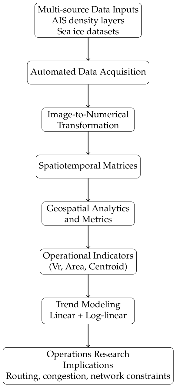
To address the limitations of purely theoretical cost models identified in the literature [9], this study proposes a data-driven framework designated as the Arctic Traffic Intelligence Framework (ATIF). Unlike traditional methodologies that rely on the procurement of raw AIS trajectory points, ATIF intentionally bypasses vector-based point clouds. Acquiring decadal, pan-Arctic historical AIS datasets from commercial providers entails significant financial barriers and massive computational infrastructure to process billions of raw signals [34,35]. By extracting numerical matrices directly from accessible rasterized density layers, our approach provides a highly cost-effective alternative, strategically sacrificing micro-level ship tracking to achieve macro-scale spatiotemporal efficiency. The methodology is structured into three sequential modules: (i) Automated Data Acquisition, focusing on the retrieval of heterogeneous raster and tabular datasets; (ii) Computer Vision & Signal Quantization, transforming visual density layers into numerical matrices; and (iii) Geospatial & Statistical Analytics, responsible for measuring route displacement and deriving the basis for operational Key Performance Indicators (KPIs). The overall architecture of the proposed framework is illustrated in Figure 1.

2.1. Maritime Traffic Dataset

The data employed in this study originate from the Global Maritime Traffic Density Service (GMTDS), operated by MapLarge [37], which provides globally aggregated representations of vessel activity derived from terrestrial and satellite Automatic Identification System (AIS) transmissions. The service processes hundreds of billions of AIS messages collected from the world’s commercial fleet, applying large-scale data validation, anomaly filtering, and trajectory reconstruction prior to spatial aggregation.

Rather than distributing individual vessel positions, the GMTDS publishes rasterized traffic density layers through an Open Geospatial Consortium (OGC)-compliant Web Map Service (WMS) [38], in which maritime activity is expressed as cumulative ship-hours per square kilometer over fixed temporal intervals. This abstraction preserves the statistical structure of global shipping flows while mitigating noise, positional uncertainty, and data sparsity inherent to raw AIS telemetry, making the dataset suitable for comparative and large-scale analyses of maritime traffic patterns.

The data ingestion module operates on two primary fronts: maritime traffic density and cryospheric indicators. For maritime traffic, we developed an automated client interacting with the MapLarge Global Maritime Traffic Density Service (GMTDS) via the WMS standard. The system queried the ais:density layer monthly from January 2012 to September 2024. To ensure spatial consistency in high latitudes, all requests were forced to the NSIDC Sea Ice Polar Stereographic North projection (EPSG:3995). This projection minimizes distortion near the pole, which is critical for accurate geometric measurements [39]. The acquisition parameters were standardized to a resolution of $2048\times 2048$ pixels with a fixed Bounding Box (BBOX) covering a radius of 3000 km from the North Pole, ensuring pixel-to-pixel correspondence throughout the entire time series.

Simultaneously, sea ice data was retrieved from the National Snow and Ice Data Center (NSIDC), specifically the NOAA/NSIDC G02135 dataset (Version 4.0) [40]. We implemented a script to programmatically harvest monthly sea ice extent values (${10}^6{\mathrm{km}}^2$), filtering for the Northern Hemisphere and synchronizing the temporal index with the maritime traffic dataset.

2.2. Visual-to-Numerical Transformation Engine

A critical challenge in using WMS data for quantitative analysis is that the output is visual (RGB images) rather than numerical [41]. To overcome this, we developed a Color-Space Interpolation Algorithm (implemented in the DensityConverter module).

The algorithm maps the Blue-Green-Red (BGR) color values of each pixel $P_{ij}$ to a vessel density value $D_{i,j}$ based on a calibrated reference scale provided by the data source. Since compression artifacts or anti-aliasing in WMS images generate colors that do not perfectly match the legend, we employed a weighted nearest-color interpolation in the 3D RGB space.

For any given pixel color $C_{obs}$, the estimated density V is calculated by finding the two nearest reference colors $C_1$ and $C_2$ in the Euclidean space (Equation (1)):

$$d_k={\parallel C_{obs}-C_k\parallel }^2$$

(1)

where $d_k$ is the squared Euclidean distance for each nearest reference color. The distances are then used to compute the interpolated density value $V\left(C_{obs}\right)$ (Equation (2)):

$$V\left(C_{obs}\right)={\displaystyle \frac{v_1·d_2+v_2·d_1}{d_1+d_2}}$$

(2)

where $v_k$ is the reference density value for each nearest reference color. This process converts the raw imagery into a sequence of scalar matrices $M_t$, where each cell represents the navigational intensity at time t.

Validation and Sensitivity Analysis Framework

To rigorously validate the Color-Space Interpolation Algorithm and assess the propagation of uncertainties caused by visual and spatial artifacts, a direct validation and sensitivity pipeline was implemented.

First, to validate the visual-to-numerical transformation, a random spatial sample of 5000 pixels was extracted from the visual framework and compared directly against the baseline raw numerical data retrieved from the original WMS API (via GetFeatureInfo).

Second, an Uncertainty Propagation and Sensitivity Analysis was designed to evaluate the algorithm’s resilience against structural anomalies. Visual uncertainties were tested through two distinct perturbations: (1) image acquisition uncertainty, simulated by artificially perturbing the original image brightness by $\pm 5\%$, and (2) color interpolation resilience, challenged by injecting artificial RGB noise (+5 channels) into the sampled pixels. Finally, geospatial projection sensitivity was evaluated by reprojecting the baseline spatial queries from the Universal Polar Stereographic projection (EPSG:3995) to the standard Web Mercator (EPSG:3857) to quantify the impact of spatial distortion on the extraction accuracy.

2.3. Geospatial Transformation and Operational Metrics

To transition from image coordinates $(i,j)$ to geodetic coordinates $(\lambda ,\varphi )$, an inverse projection mechanism was applied using the pyproj library. The centroids of high-density clusters were re-projected from the EPSG:3995 plane to WGS84 (EPSG:4326), allowing for the calculation of geodetic distances.

Based on the homogenized matrices, three primary operational metrics were defined:

Real Volume Index ($V_R$): a proxy for total physical maritime traffic, calculated as the sum of density values weighted by the true geographical area of each pixel across the navigable matrix, as presented in Equation (3):

$$V_R\left(t\right)=\sum _{i,j}{M}_t(i,j)\times A(i,j)$$

(3)

where $A(i,j)$ is the geodetic area, in ${\mathrm{km}}^2$, on the WGS84 ellipsoid corresponding to the pixel at position $(i,j)$.

Navigable Area ($A_N$): the total spatial footprint of active shipping lanes, calculated by summing the precise ellipsoidal area of all non-zero pixels (Equation (4)):

$$A_N\left(t\right)=\sum _{i,j}\mathbb{I}(M_t(i,j)>0)\times A(i,j)$$

(4)

where $\mathbb{I}$ is the indicator function that equals 1 if the condition is met and 0 otherwise.

Route Centroid Displacement ($C_G$): to test the hypothesis of routes migrating northward, we calculate the weighted geographic center of the traffic mass. To prevent spatial distortions inherent to 2D planar projections, the geodetic coordinates (latitude $\varphi$ and longitude $\lambda$) of each active pixel were first mathematically converted into 3D Earth-Centered, Earth-Fixed (ECEF) Cartesian coordinates ($X,Y,Z$) based on the WGS84 reference ellipsoid parameters. The spatial centroid was then computed directly in the three-dimensional space, weighted by the real physical volume (density × true ellipsoidal area) of each pixel, as given in Equation (5):

$$C_G\left(t\right)={\displaystyle \frac{{\sum }_{i,j}{M}_t(i,j)\times A(i,j)\times {\mathbf{r}}_{i,j}}{V_R\left(t\right)}}$$

(5)

where ${\mathbf{r}}_{i,j}$ represents the 3D Cartesian position vector $(X,Y,Z)$ of the pixel at coordinates $(i,j)$, and the denominator $V_R\left(t\right)$ is the Real Volume Index acting as the total mass for the centroid calculation. For geographic representation, the resulting centroid coordinates were transformed back into geodetic latitude and longitude on the WGS84 ellipsoid using the standard inverse geodetic transformation.

To ensure robustness, all metrics were consistently evaluated across time series using fixed spatial resolution, projection parameters, and color reference scales, preventing artifacts from heterogeneous data sources. The resulting framework enables a direct empirical assessment of how Arctic navigation intensity, spatial extent, and route geometry have evolved under changing cryospheric conditions.

2.4. Trend Estimation

To quantify and interpret temporal changes in navigation intensity across the Arctic, we applied two distinct trend modeling approaches at the pixel level: an absolute linear trend model and a relative log-linear trend model. These approaches capture complementary aspects of change over time and are motivated by different assumptions about the underlying process.

2.4.1. Absolute Linear Trend

We first estimated a simple linear regression for each pixel (Equation (6)) [42]:

$$y_t=\alpha +\beta t+{\epsilon }_t$$

(6)

where $y_t$ is the observed navigation intensity at time t, $\alpha$ is the intercept, $\beta$ is the slope representing the absolute change per time unit and ${\epsilon }_t$ are residuals. This model provides a direct measure of how much the metric increases or decreases in absolute units per year.

The linear trend model is widely used in time series analysis when the primary interest lies in an absolute increment, such as evaluating whether a variable has undergone a systematic upward or downward change in its original units. This model is conceptually simple, interpretable, and provides a baseline against which more complex or transformed models can be compared.

However, in environmental and observational datasets such as navigation counts or intensities, absolute changes may be misleading when baseline levels differ substantially across pixels. For example, a pixel with low baseline activity may show a small absolute change that is proportionally large, while a pixel with high baseline activity may show a larger absolute change that is proportionally small. The linear slope $\beta$ does not adjust for such baseline differences, which can obscure meaningful relative dynamics in spatial comparisons.

2.4.2. Relative Log-Linear Trend and Annual Percentage Change

To address the limitations of absolute trend estimation, we also fitted a log-linear trend model [28] using a log-plus-one transformation. Because maritime traffic data frequently contains zero-value observations (e.g., in non-navigable areas, sea ice constraints, or during off-season months) and $ln\left(0\right)$ is mathematically undefined, shifting the intensity values by one unit prevents mathematical indefiniteness. This approach elegantly preserves the zero-traffic semantics, as $ln\left(1\right)=0$, allowing the regression to proceed over the entire spatial grid. The updated specification is shown in Equation (7):

$$ln(y_t+1)=\alpha +\beta t+{\epsilon }_t$$

(7)

In this specification, the transformed natural logarithm of the navigation intensity is regressed in time. This transformation converts multiplicative changes on the original scale into additive changes on the log scale. Log transformations are standard practice when proportional rather than absolute changes are of interest, stabilizing variance and linearizing exponential or growth-like processes.

The key advantage of the log-linear model is that the coefficient $\beta$ represents a constant proportional (multiplicative) rate of change. This is particularly appropriate for variables that evolve relative to their magnitude and facilitates comparison across spatial units with heterogeneous baseline levels.

To interpret $\beta$ in terms of an annual percentage change (APC) in the original navigation intensity scale, we apply the standard exponential back-transformation (Equation (8)) [28]:

$$\mathrm{APC}=\left(e^{\beta }-1\right)\times 100$$

(8)

This transformation yields an exact estimate of the mean percent change per year implied by the log-linear model. Positive APC values indicate a growth trend, while negative APC values indicate a decline. APC estimation via log regression is a well-established technique in longitudinal trend analysis across disciplines, including epidemiology and environmental change research, where proportional effects are central to interpretation.

The linear model (Equation (6)) captures absolute change, whereas the log-linear specification (Equation (7)) allows the estimation of proportional variation, expressed as the annual percentage change (Equation (8)). Using both absolute and relative trend measures provides a multi-faceted understanding of temporal change. The absolute trend ($\beta$) highlights areas with the largest net increases or decreases in navigation intensity in the original units, which is useful for detecting broad structural changes in traffic volume over time.

In contrast, the relative trend (APC) highlights areas where the navigation intensity is changing the fastest in proportional terms, regardless of the baseline activity. In the Arctic context, this distinction is especially important for identifying emergent routes or rapid growth in less trafficked regions that may be overlooked when only absolute trends are considered.

Combined, these models allow for a richer interpretation of both the magnitude and rate of change, addressing potential biases introduced by spatial heterogeneity in baseline navigation intensity. Such complementary analysis strengthens inferences about the spatial dynamics of shipping and the influence of seasonal ice retreat patterns on route development.

3. Results

The deployment of ATIF from 2012 to 2024 generated a comprehensive spatiotemporal dataset. To ensure spatial accuracy at high latitudes, all density metrics incorporate the calculation of the geodesic area for each individual pixel based on its geodetic coordinates. This allowed for the isolation of navigational trends that were previously obscured in aggregated economic statistics. The results are presented in three dimensions: temporal seasonality, climatic correlation, and spatial displacement.

3.1. Quantitative Validation of the Transformation Engine

The empirical validation of the visual-to-numerical conversion demonstrated high fidelity in the data recovery process. When comparing the extracted pixel values against the raw WMS API data, the algorithm exhibited a controlled Mean Absolute Error (MAE) of 0.8353 vessels/km² and a Root Mean Square Error (RMSE) of 3.6237 vessels/km². This indicates that while minor edge-effect anomalies exist due to visual smoothing, the overall average deviation remains minimal. Crucially, the spatial hierarchy and structural integrity of the traffic networks are perfectly preserved, as evidenced by a near-perfect Spearman’s rank correlation ($\rho =0.9997$) and a strong Lin’s Concordance Correlation Coefficient (CCC $=0.8355$). These metrics confirm the framework’s efficacy and reliability for macro-scale spatiotemporal analysis.

3.2. Uncertainty Propagation and Sensitivity Analysis

The evaluation of worst-case scenarios for visual artifacts and spatial projection constraints confirmed the robustness of the data-driven approach. Regarding visual uncertainties, the algorithm maintained exceptional stability under image brightness perturbations ($\pm 5\%$). The MAE remained highly constrained (fluctuating between 0.39 and 0.56 vessels/km²), and the Pearson correlation remained remarkably high ($r>0.97$). Against simulated anti-aliasing artifacts (injected RGB noise), the pipeline demonstrated strong fault tolerance, preserving Lin’s CCC of 0.8955. These tests empirically prove that the extraction method successfully prevents minor visual errors, such as image compression and monitor calibration variances, from propagating into the final linear trend statistics.

Furthermore, the geospatial projection sensitivity test underscored the absolute necessity of spatial integrity. Reprojecting the queries to the standard Web Mercator projection (EPSG:3857)—a widely used but highly inadequate projection for polar regions—resulted in a severe propagation of spatial distortion. Under the Mercator scenario, the correlation completely collapsed (Pearson $r=0.17$; Lin CCC $=0.09$), and the error nearly doubled to 0.8284 vessels/km². This test empirically validates our methodological framework, proving that the strict utilization of the Universal Polar Stereographic projection (EPSG:3995) is a fundamental mathematical requirement to maintain the baseline’s near-perfect accuracy and prevent spatial uncertainty propagation.

3.3. Bilateral Expansion of the Operational Window

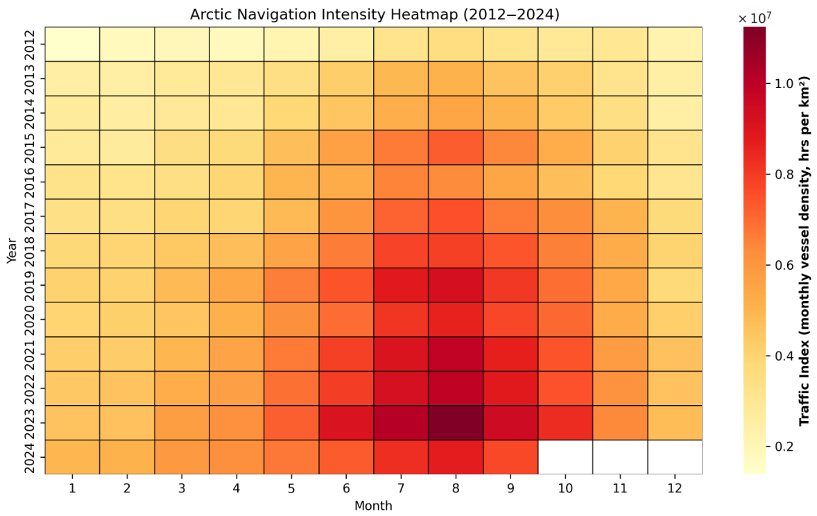
The longitudinal analysis of traffic density reveals a structural shift in the phenology of Arctic navigation. As illustrated in Figure 2, the “high-intensity window”, defined as periods where normalized traffic density exceeds the 0.7 threshold (red zones), has expanded significantly at both seasonal termini.

In the early phase of the time series (2012–2015), the operational window was strictly confined. Notably, the early summer period (June/Month 6) was characterized by low-density activity (represented by yellow/pale orange hues), indicating that remnant winter ice continued to impede navigation. Contrastingly, the 2020–2024 data exhibit a comprehensive widening of the season.

Spring onset (early entry): There is a marked intensification in traffic during June (Month 6). In 2023, this month exhibits density levels (orange/red) comparable to the peak summer months of previous years. This empirical evidence suggests an earlier retreat of the ice edge, allowing vessels to penetrate the High North weeks earlier than in the previous decade.

Autumn extension (late exit): Simultaneously, the navigation season has extended into late October (Month 10), driven by the thermal inertia of the open ocean, which delays freeze-up.

3.4. Climatic Sensitivity

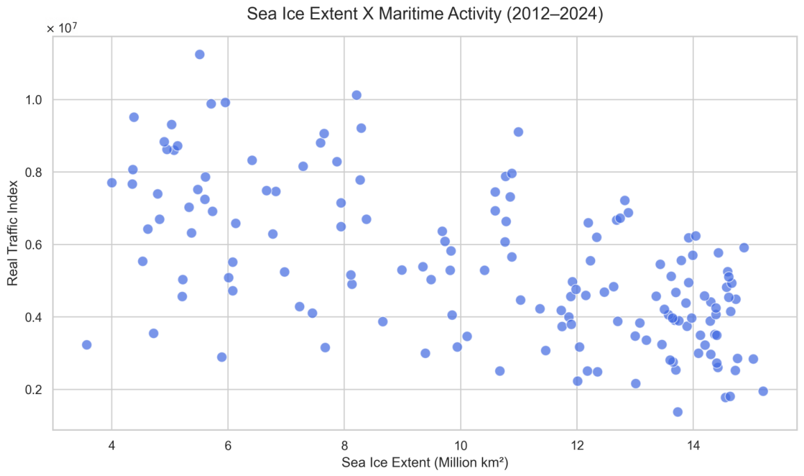
To evaluate the dependency of maritime logistics on cryospheric conditions, we analyzed the dispersion between Sea Ice Extent (${10}^6$ km²) and the extracted Real Traffic Index ($V_R$). As illustrated in Figure 3, the scatter plot reveals a clear macroscopic trend: lower sea ice extents are visibly associated with higher volumes of maritime activity. This behavioral coherence further validates ATIF’s capacity to accurately capture expected physical dynamics from visual data.

However, the dispersion also highlights that sea ice retreat is an enabler rather than an absolute determinant. Notably, the data exhibits instances of substantial navigational intensity even during periods of relatively high ice extent. This variation is a critical finding: it confirms that while the physical retreat of the cryosphere acts as the primary gatekeeper—establishing the baseline accessibility for logistics networks—the actual volume of traffic is progressively decoupling from strict climatic constraints. The persistence of high traffic in harsher conditions suggests that non-climatic factors, such as sustained economic demand, strategic resource extraction, and the utilization of heavy icebreakers or high ice-class vessels, are playing an increasingly dominant role in Arctic operations.

3.5. Displacement of the Geometric Navigational Centroid

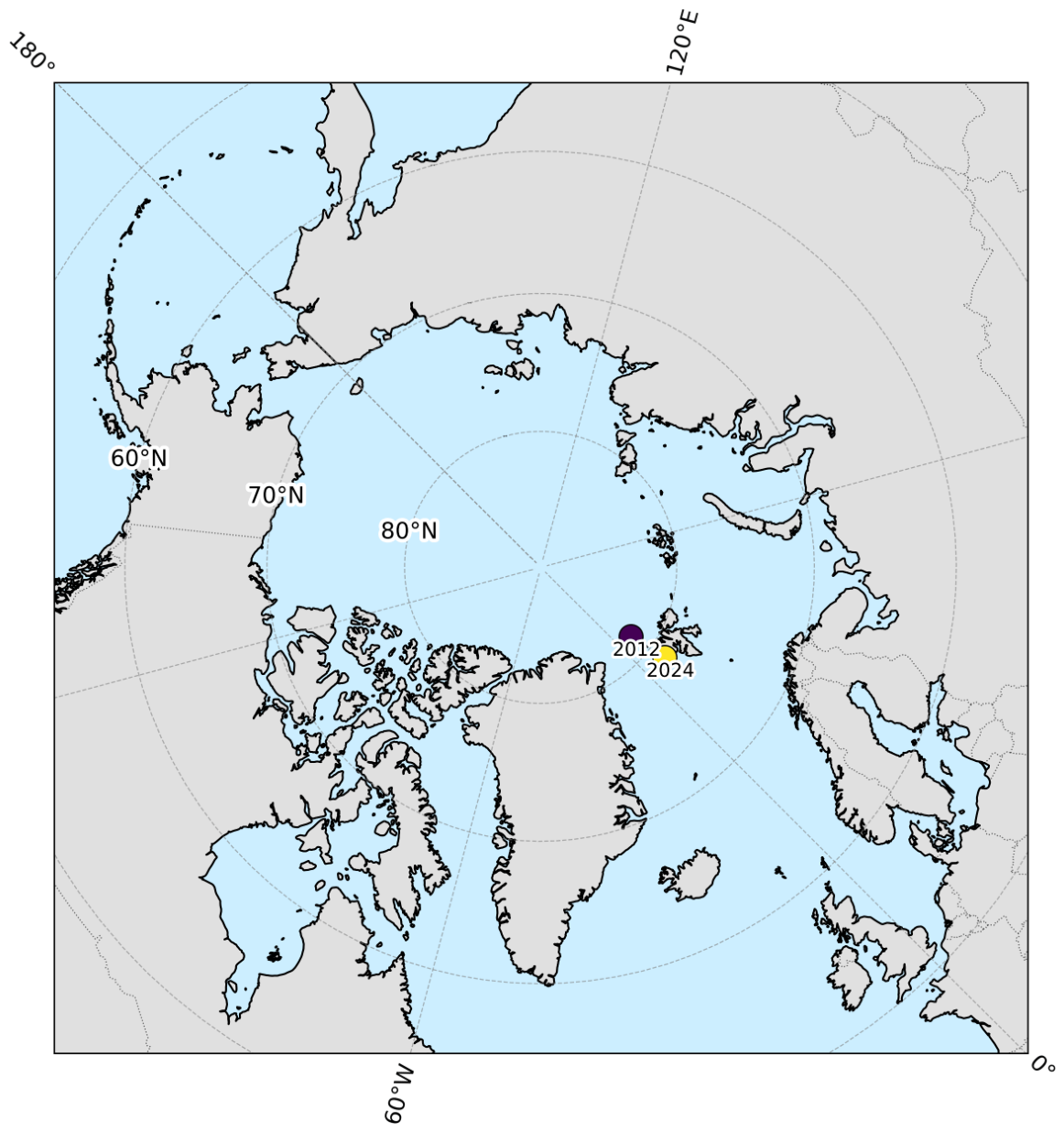
Contrary to the hypothesis that receding ice would immediately trigger a migration toward high-latitude transpolar routes, the geometric centroid analysis (Figure 4) reveals a counter-intuitive southeastward displacement.

In 2012, the navigational “center of gravity” was located deeper within the Arctic Basin. By 2024, this centroid has shifted markedly toward the Atlantic Gateway (approximating the Barents/Greenland Sea interface). This trajectory indicates that the sheer volume of maritime activity is consolidating around the western entry points rather than spreading across the pole.

3.6. Monthly Phenology and Regional Asymmetry

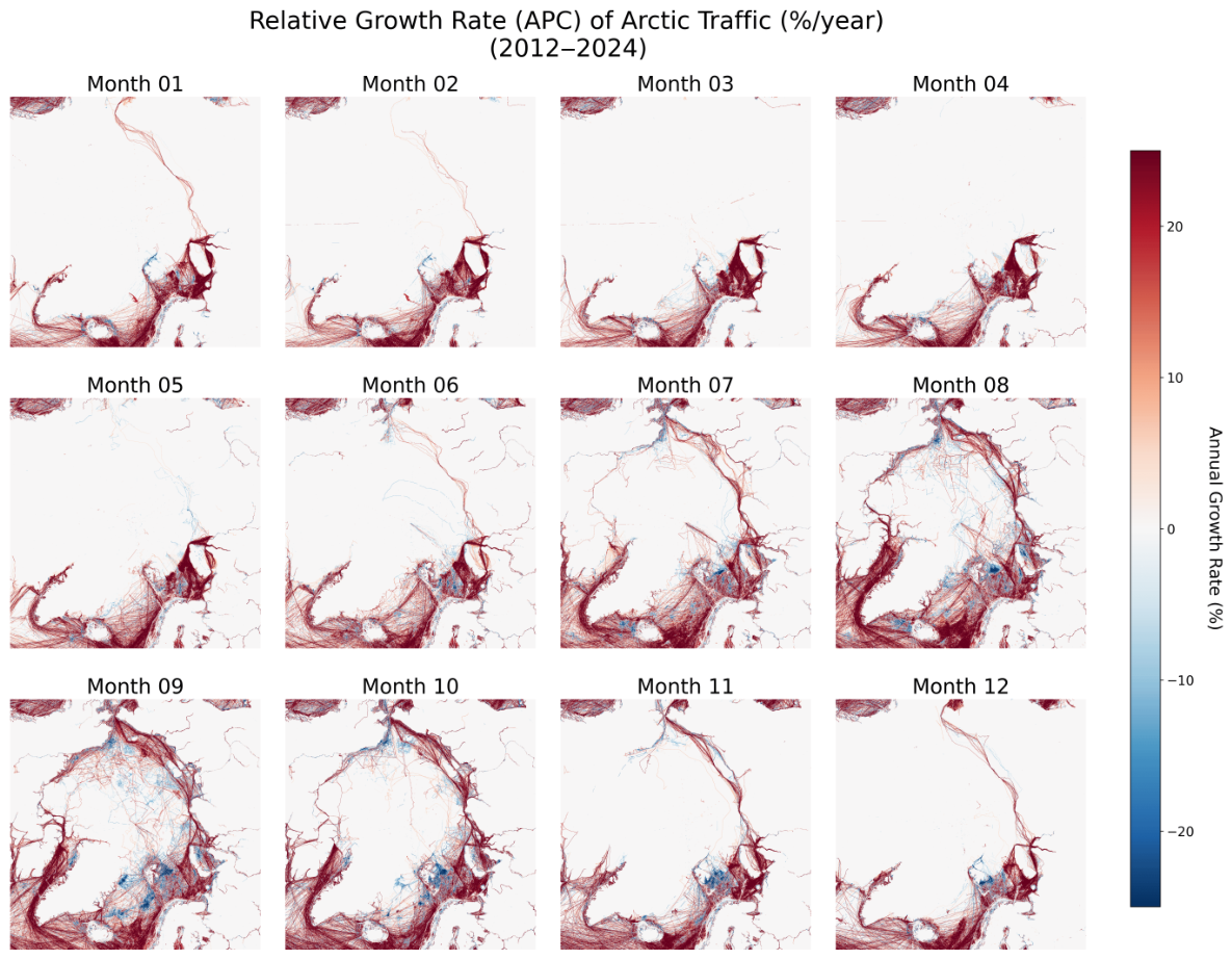
While the aggregated annual data indicates general growth, the decomposition of growth rates by month (Figure 5) uncovers a distinct phenological pattern in which intensification occurs. The monthly panels reveal that the highest growth rates (dark red trajectories, >15% APC) are not evenly distributed throughout the open-water season. Instead, they are clustered in the late-season window (August–November) specifically along the Northern Sea Route (NSR).

Summer peak (Months 7–9): the mid-summer months show a consolidated high-growth corridor along the Siberian coast, confirming the maturing of the NSR as a transit artery.

Shoulder season (Months 10–11): crucially, the growth remains positive and intense well into November in the Kara and Barents Seas. This visualizes the operational impact of the “Atlantic Pull” mentioned in Section 3.3, where ice-strengthened tankers continue export operations despite the onset of winter darkness.

3.7. Structural Dichotomy: Technical Viability vs. Economic Reality

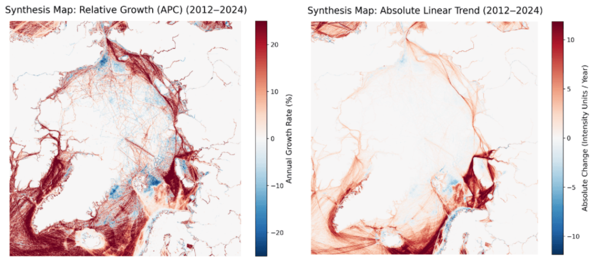
To further dissect the nature of this expansion, we applied the dual-trend methodology defined in Section 2.4. Figure 6 juxtaposes the Relative Growth (APC) against the Absolute Linear Trend, revealing a critical asymmetry in Arctic accessibility.

The Relative Growth Map exhibits a continuous, high-intensity trajectory (red hue > 15% APC) stretching across the entire longitudinal span of the Russian Arctic, from the Kara Gate to the Bering Strait. This signals a systemic activation of the route: regions that historically saw near-zero traffic in the Eastern Siberian Sea are now experiencing consistent transit activity. From a purely navigational perspective, this confirms that the “trans-Arctic” corridor is technically open and operational.

However, the Absolute Linear Trend Map provides a sobering counter-narrative regarding economic volume. The intensity of physical shipping mass (ship-hours/km²) remains heavily concentrated in the western sector (Barents and Kara Seas), coinciding with the location of major hydrocarbon extraction terminals (e.g., Yamal LNG, Arctic LNG 2). As one moves eastward past the Taymyr Peninsula, the absolute trend fades significantly.

4. Discussion

4.1. The Role of Ice vs. Economic Drivers

The observed bilateral expansion (earlier break-up and delayed freeze-up)confirms the accelerated accessibility projections made by Melia et al. [7], demonstrating that the Arctic is rapidly transitioning from a seasonally restricted zone to a region with a semi-permanent navigable window of nearly 5 months (June–October).

However, the remaining variance in our climatic sensitivity model suggests that once this physical barrier is lifted, other drivers accelerate the utilization of the route. This aligns with the “resource-based” model described by Gunnarsson & Moe [43]. Their analysis of the Northern Sea Route indicates that while the receding ice provides the opportunity (captured by our 35% correlation), the magnitude of traffic is amplified by large-scale industrial projects, such as the Yamal LNG exports, and state tariff policies. Thus, our data confirm a dual-driver system: ice retreat dictates the possibility of navigation, while economic contracts dictate the intensity of the flow.

4.2. Network Topology and Regional Disparities

The spatial pattern of the geometric centroid reflects the network topology described by Eguíluz et al. [44]: the Arctic shipping network is not a uniform ring, but a highly clustered system heavily weighted towards the Atlantic. The shift suggests that the explosive growth of shuttle tankers exporting hydrocarbons to Europe statistically outweighs the volume of “transit shipping” across the Northern Sea Route, anchoring the logistic center of mass southward near existing industrial infrastructure.

In sharp contrast, the Canadian archipelago (Northwest Passage) exhibits stagnated or negative growth rates across almost all months. This regional disparity explains the geometric displacement observed: the centroid is being pulled southwestward precisely because the Russian network is expanding while the North American side remains dormant. This reinforces the findings of Lasserre [45], who characterized the Arctic not as a homogeneous region, but as a dual system: a robust, rapidly growing Russian network driven by state policy, versus a static, underdeveloped North American network.

This contrast corroborates the hypothesis that while the NSR is expanding globally (as seen in the APC), it is not yet functioning as a homogenized international trade highway. Instead, the traffic structure is dominated by destinational shipping (exporting resources from the Russian Arctic to Europe) rather than transit shipping between the Pacific and Atlantic.

4.3. Operational Implications and Network Constraints

The data validate that the Arctic is transitioning from a frontier of exploration to a standardized corridor for resource extraction. The extension of the operational window to nearly 5 months challenges the assumption that the Arctic routes are only viable for opportunistic charters.

However, the spatial concentration identified introduces a critical logistic vulnerability. Because traffic is not dispersing across the Transpolar Route but is instead consolidating in the Barents and Kara Seas, this region is becoming a high-density bottleneck. As analyzed by Jing et al. [46] using system dynamics, such non-linear growth in traffic volume significantly escalates the risk profile of the route—not only in terms of projected emissions but also regarding collision risks in ice-covered waters.

Crucially, this densification has profound human implications. As detailed in recent assessments of Arctic shipping impacts on environments and communities [47], the burden of this industrial activity falls disproportionately on local ecosystems and Indigenous populations. The convergence of heavy shipping disrupts marine migration patterns through underwater noise and introduces pollutants that compromise food security and the cultural continuity of communities reliant on subsistence hunting.

Consequently, the challenge for logistics planners has evolved to encompass not only overcoming ice (which is retreating) but also the management of traffic congestion and environmental capacity within the narrowing corridors of the Western Arctic. Future route optimization models must account for these externalities, as regulatory pressures on these high-density zones are likely to become the new limiting factor for capacity. To precisely evaluate the financial and operational impact of these new constraints, future maritime economics research can utilize the empirical data generated by ATIF as a baseline to model transit cost elasticities and quantify the changing values of shipping time.

4.4. Methodological Limitations

A limitation of this study stems from the source imagery products, which are natively provided as monthly aggregates. Consequently, aggregating the data to monthly intervals inherently smooths out sub-monthly phenomena, such as weekly weather disruptions or immediate ice-breaker convoy dependencies, which are critical for tactical operational planning. While tactical, short-term planning would require alternate, raw-telemetry pipelines, this frequency matches the strategic focus of our analysis.

5. Conclusions

The deployment of ATIF and the application of log-linear regression to the 2012–2024 dataset provide a robust quantitative basis for understanding the evolution of Arctic maritime logistics and enhancing operational research in this region. The findings challenge the assumption of a uniform “Transpolar” opening, revealing instead a highly asymmetrical development pattern.

First, the phenological analysis confirms a structural shift in accessibility. The operational window has expanded bilaterally, effectively creating a semi-permanent navigable season from June to October. This extension is driven not only by the physical retreat of the ice edge but also by the thermal inertia of the open ocean, which delays freeze-up and supports late-season navigation. For logistics planners, this shift redefines the temporal constraints of scheduling algorithms, allowing for extended shipping campaigns previously deemed infeasible.

Spatially, the divergence between Absolute Trends and Relative Growth (APC) identifies a critical vulnerability. While the route is technically open longitudinally, the operational reality is a massive consolidation of shipping volume in the Barents and Kara Seas. This “Atlantic Pull” has displaced the geometric centroid of navigation southwestward, creating a high-density bottleneck in the western Arctic while the North American sector remains comparatively stagnant.

Consequently, these dynamics imply that the primary challenge for future Arctic logistics is no longer simply traversing ice-covered waters, but managing congestion in narrowing operational corridors. The non-linear growth in traffic density significantly escalates the risks of collision and environmental impact on local communities, suggesting that regulatory capacity and environmental governance, rather than ice thickness, will become the new binding constraints for route development. Future operational research must therefore evolve from deterministic ice-avoidance models to stochastic congestion frameworks, integrating these externalities into multi-objective optimization algorithms to ensure sustainable network capacity.

From an operations research standpoint, the observed traffic concentration and the emergence of regional bottlenecks suggest the need for stochastic network optimization models incorporating seasonal accessibility constraints and congestion effects. Future work may formalize these dynamics through multi-objective routing models, equilibrium frameworks, or game-theoretic formulations capable of capturing strategic interactions between shipping operators and regulatory authorities in a changing Arctic environment.

References

1. Liu, H.; Mao, Z.; Zhang, Z. From melting ice to green shipping: Navigating emission reduction challenges in Arctic shipping in the context of climate change. Front. Environ. Sci. 2024, 12, 1462623. [Google Scholar] [CrossRef]
2. Smith, L.C.; Stephenson, S.R. New Trans-Arctic Shipping Routes Navigable by Midcentury. Proc. Natl. Acad. Sci. USA 2013, 110, E1191–E1195. [Google Scholar] [CrossRef] [PubMed]
3. Stephenson, S.R.; Smith, L.C.; Agnew, J.A. Divergent Long-Term Trajectories of Human Access to the Arctic. Nat. Clim. Chang. 2011, 10, 156–160. [Google Scholar] [CrossRef]
4. Stephenson, S.; Smith, L. Influence of Climate Model Variability on Projected Arctic Shipping Futures. Earth’s Future 2015, 3, 331–343. [Google Scholar] [CrossRef]
5. Stephenson, S.; Wang, W.; Zender, C.; Wang, H.; Davis, S.; Rasch, P. Climatic Responses to Future Trans-Arctic Shipping. Geophys. Res. Lett. 2018, 45, 9898–9908. [Google Scholar] [CrossRef] [PubMed]
6. Aksenov, Y.; Popova, E.E.; Yool, A.G.N.A.; Williams, T.D.; Bertino, L.; Bergh, J.; Bergh, J. On the Future Navigability of Arctic Sea Routes: HighResolution Projections of the Arctic Ocean and Sea Ice. Mar. Policy 2017, 75, 300–317. [Google Scholar] [CrossRef]
7. Melia, N.; Haines, K.; Hawkins, E. Sea Ice Decline and 21st Century Trans-Arctic Shipping Routes. Geophys. Res. Lett. 2016, 43, 9720–9728. [Google Scholar] [CrossRef]
8. Shu, Y.; Cui, H.; Song, L.; Gan, L.; Xu, S.; Wu, J.; Zheng, C. Influence of sea ice on ship routes and speed along the Arctic Northeast Passage. Ocean Coast. Manag. 2024, 256, 107320. [Google Scholar] [CrossRef]
9. Theocharis, D.; Rodriguez, J.P.; Pettit, S.; Beresford, A. Arctic shipping: A systematic literature review of comparative studies. J. Transp. Geogr. 2018, 69, 112–128. [Google Scholar] [CrossRef]
10. Kandel, R.; Baroud, H. A data-driven risk assessment of Arctic maritime incidents. Reliab. Eng. Syst. Saf. 2024, 243, 109779. [Google Scholar] [CrossRef]
11. Yang, X.; Lin, Z.Y.; Zhang, W.J.; Xu, S.; Zhang, M.Y.; Wu, Z.D.; Han, B. Review of risk assessment for navigational safety in Arctic waters. Ocean Coast. Manag. 2024, 247, 106931. [Google Scholar] [CrossRef]
12. Schoyen, H.; Braathen, S. The Northern Sea Route versus the Suez Canal. J. Transp. Geogr. 2011, 19, 977–983. [Google Scholar] [CrossRef]
13. Makarov, D.; Makarova, O.; Mayurov, N.; Mayurov, P.; Turova, V. Development prospects and importance of the Northern Sea Route. Transp. Res. Procedia 2022, 63, 1114–1120. [Google Scholar] [CrossRef]
14. Cheaitou, A.; Cariou, P. Greening of maritime transportation: A multi-objective optimization approach. Ann. Oper. Res. 2019, 273, 501–525. [Google Scholar] [CrossRef]
15. Tu, E.; Zhang, G.; Rachmawati, L.; Rajabally, E.; Huang, G.B. Exploiting AIS Data for Intelligent Maritime Navigation: A Comprehensive Survey From Data to Methodology. IEEE Trans. Intell. Transp. Syst. 2018, 19, 1559–1582. [Google Scholar] [CrossRef]
16. Yang, D.; Wu, L.; Wang, S.; Jia, H.; Li, K.X. How big data enriches maritime research—A critical review of Automatic Identification System (AIS) data applications. Transp. Rev. 2019, 39, 755–773. [Google Scholar] [CrossRef]
17. Duka, A.; Zhang, H.; Vidan, P.; Li, G. Exploring Recent Maritime Research on AIS-Based Ship Behavior Analysis and Modeling. J. Mar. Sci. Eng. 2026, 14, 712. [Google Scholar] [CrossRef]
18. Wright, D.; Janzen, C.; Bochenek, R.; Austin, J.; Page, E. Marine Observing Applications Using AIS: Automatic Identification System. Front. Mar. Sci. 2019, 6, 537. [Google Scholar] [CrossRef]
19. Wang, Y.; Liu, R.W.; Liu, J.; Yang, L.; Liu, Y. AIS Data-Driven Maritime Traffic Flow Prediction and Density Visualization Using Multitime Scale Temporal Feature Fusion Network. IEEE Sens. J. 2025, 25, 11357–11365. [Google Scholar] [CrossRef]
20. Liu, L.; Shibasaki, R.; Zhang, Y.; Kosuge, N.; Zhang, M.; Hu, Y. Data-driven framework for extracting global maritime shipping networks by machine learning. Ocean Eng. 2023, 269, 113494. [Google Scholar] [CrossRef]
21. Jin, L.; Chen, J.; Chen, Z.; Sun, X.; Yu, B. Impact of COVID-19 on China’s international liner shipping network based on AIS data. Transp. Policy 2022, 121, 90–99. [Google Scholar] [CrossRef] [PubMed]
22. Yang, H.; Liu, C.; Cao, Y.; Shu, Y.; Gan, L.; Liu, Z.; Yang, Z. Dynamic resilience assessment of global shipping networks against cascading effects: An AIS data-driven complex network analysis. Sustain. Horiz. 2026, 18, 100184. [Google Scholar] [CrossRef]
23. Kim, H.S.; Lee, E.; Lee, E.J.; Hyun, J.W.; Gong, I.Y.; Kim, K.; Lee, Y.S. A Study on Grid-Cell-Type Maritime Traffic Distribution Analysis Based on AIS Data for Establishing a Coastal Maritime Transportation Network. J. Mar. Sci. Eng. 2023, 11, 354. [Google Scholar] [CrossRef]
24. Liu, Z.; Gao, H.; Zhang, M.; Yan, R.; Liu, J. A data mining method to extract traffic network for maritime transport management. Ocean Coast. Manag. 2023, 239, 106622. [Google Scholar] [CrossRef]
25. Yim, J.; Kim, W.H.; Cho, S.J.; Kim, C.W.; Park, J.Y. Investigating maritime traffic routes: Integrating AIS data and topographic statistics. Marit. Policy Manag. 2025, 52, 590–608. [Google Scholar] [CrossRef]
26. Kim, Y.J.; Lee, J.S.; Pititto, A.; Falco, L.; Lee, M.S.; Yoon, K.K.; Cho, I.S. Maritime Traffic Evaluation Using Spatial-Temporal Density Analysis Based on Big AIS Data. Appl. Sci. 2022, 12, 11246. [Google Scholar] [CrossRef]
27. Yang, J.; Bian, X.; Qi, Y.; Wang, X.; Yang, Z.; Liu, J. A spatial-temporal data mining method for the extraction of vessel traffic patterns using AIS data. Ocean Eng. 2024, 293, 116454. [Google Scholar] [CrossRef]
28. Li, G.; Zhang, X.; Jiang, L.; Wang, C.; Huang, R.; Liu, Z. An approach for traffic pattern recognition integration of ship AIS data and port geospatial features. Geo-Spat. Inf. Sci. 2024, 27, 2048–2075. [Google Scholar] [CrossRef]
29. Wang, P.; Wen, Y.; Ai, B.; Liu, X. Spatial pattern and coupling characteristics analysis of maritime traffic and economic development based on shipping big data. Front. Mar. Sci. 2024, 11, 1410885. [Google Scholar] [CrossRef]
30. Hu, W.; Cervone, G.; Trusel, L.; Yu, M. Arctic accessibility: Recent trend in observed ship tracks and validation of arctic transport accessibility model. Ann. GIS 2024, 30, 455–474. [Google Scholar] [CrossRef]
31. Liu, Y.; Luo, H.; Min, C.; Chen, Q.; Yang, Q. Changes in the Arctic Traffic Occupancy and Their Connection to Sea Ice Conditions from 2015 to 2020. Remote Sens. 2024, 16, 1157. [Google Scholar] [CrossRef]
32. Openshaw, S. The Modifiable Areal Unit Problem. In Concepts and Techniques in Modern Geography (CATMOG); Geo Books: Norwich, UK, 1983; Volume 38. [Google Scholar]
33. Silber, G.K.; Adams, J.D. Vessel Operations in the Arctic, 2015–2017. Front. Mar. Sci. 2019, 6, 573. [Google Scholar] [CrossRef]
34. Lensu, M.; Goerlandt, F. Big Maritime Data for the Baltic Sea with a Focus on the Winter Navigation System. Mar. Policy 2019, 104, 53–65. [Google Scholar] [CrossRef]
35. Fiorini, M.; Capata, A.; Bloisi, D. Ais Data Visualization for Maritime Spatial Planning (MSP). Int. J. E-Navig. Marit. Econ. 2016, 5, 45–60. [Google Scholar] [CrossRef]
36. Xiao, F.; Ligteringen, H.; Gulijk, C.; Ale, B. Comparison Study on AIS Data of Ship Traffic Behavior. Ocean Eng. 2015, 95, 84–93. [Google Scholar] [CrossRef]
37. MapLarge Inc. Global Maritime Traffic Density Service (GMTDS): Technical Integration Guide; MapLarge Inc.: Atlanta, GA, USA, 2023. [Google Scholar]
38. Open Geospatial Consortium. OpenGIS Web Map Service (WMS) Implementation Specification; Technical Report OGC Document 06-042; Open Geospatial Consortium: Arlington, VA, USA, 2006. [Google Scholar]
39. Snyder, J.P. Map Projections: A Working Manual; U.S. Geological Survey Professional Paper 1395; U.S. Government Printing Office: Washington, DC, USA, 1987.
40. Fetterer, F.; Knowles, K.; Meier, W.N.; Savoie, M.; Windnagel, A.K. Sea Ice Index, Version 4; National Snow and Ice Data Center: Boulder, CO, USA, 2025. [CrossRef]
41. Gonzalez, R.C.; Woods, R.E. Digital Image Processing, 4th ed.; Pearson: New York, NY, USA, 2018. [Google Scholar]
42. Mudelsee, M. Trend analysis of climate time series: A review of methods. Earth-Sci. Rev. 2019, 190, 310–322. [Google Scholar] [CrossRef]
43. Gunnarsson, B.; Moe, A. Ten years of international shipping on the Northern Sea Route: Trends and challenges. Arct. Rev. Law. Politics 2021, 12, 4–30. [Google Scholar] [CrossRef]
44. Eguíluz, V.M.; Fernández-Gracia, J.; Irigoien, X.; Duarte, C.M. A quantitative assessment of Arctic shipping in 2010–2014. Sci. Rep. 2016, 6, 30682. [Google Scholar] [CrossRef] [PubMed]
45. Lasserre, F. Arctic shipping: A contrasted expansion of a largely destinational market. In The Global Arctic Handbook; Springer: Cham, Switzerland, 2018. [Google Scholar] [CrossRef]
46. Jing, D.; Dai, L.; Hu, H.; Ding, W.; Wang, Y.; Zhang, M. CO2 emission projection for Arctic shipping: A system dynamics approach. Ocean Coast. Manag. 2021, 205, 105531. [Google Scholar] [CrossRef]
47. Huntington, H.P.; Olsen, J.; Zdor, E.; Zagorskiy, A.; Shin, H.C.; Romanenko, O.; Kaltenborn, B.; Dawson, J.; Davies, J.; Abou-Abbsi, E. Effects of Arctic commercial shipping on environments and communities. Transp. Res. Part D 2023, 118, 103731. [Google Scholar] [CrossRef]
Figure 1. Arctic Traffic Intensity Framework (ATIF). The proposed pipeline integrates multi-source data acquisition, visual-to-numerical conversion, and geospatial analytics to generate spatiotemporal indicators of Arctic navigation dynamics and inform operations research models for emerging polar logistics networks.
Jmse 14 01236 g001
Figure 2. Arctic navigation heatmap: high-intensity window expansion.
Jmse 14 01236 g002
Figure 3. Scatter plot illustrating the impact of Sea Ice Extent on the Real Traffic Index. The dispersion shows a general trend of increased activity during ice retreat, alongside notable high-traffic instances in higher ice conditions.
Jmse 14 01236 g003
Figure 4. Displacement of the navigational centroid.
Jmse 14 01236 g004
Figure 5. Annual growth rate of Arctic maritime traffic (%/year) between 2012 and 2024: decomposition by month.
Jmse 14 01236 g005
Figure 6. Relative Growth (APC, (left)) vs. Absolute Linear Trend (right).
Jmse 14 01236 g006
Disclaimer/Publisher’s Note: The statements, opinions and data contained in all publications are solely those of the individual author(s) and contributor(s) and not of MDPI and/or the editor(s). MDPI and/or the editor(s) disclaim responsibility for any injury to people or property resulting from any ideas, methods, instructions or products referred to in the content.