AIS-Based Ship Trajectory Prediction Using a Geometry-Consistent Trajectory Transformer (GCT-Former)

Abstract

Accurate vessel trajectory prediction from Automatic Identification System (AIS) records is important for maritime traffic monitoring, route planning, and intelligent vessel traffic management. However, reliable prediction remains challenging for long forecasting horizons and turning maneuvers. To address this problem, this study proposes the Geometry-Consistent Trajectory Transformer (GCT-Former), a progressive and refinement-based framework for AIS-based vessel trajectory prediction. The proposed model integrates multi-scale historical trajectory encoding, progressive residual future-position generation, and global–local trajectory refinement to improve the stability and continuity of long-horizon trajectory prediction. The predicted trajectories are evaluated as geometric future-position estimates and can provide trajectory-level information for downstream maritime traffic monitoring and decision-support applications. Experiments are conducted on three real-world Danish maritime regions: Aarhus Bay, Great Belt, and Skagen. Compared with representative conventional and deep-learning trajectory prediction models, the proposed model shows its most consistent advantage in long-horizon prediction, particularly in terms of ADE and FDE. In the long-term setting, it achieves average displacement errors of 0.344, 0.546, and 0.218 km and final displacement errors of 0.774, 1.368, and 0.525 km on Aarhus Bay, Great Belt, and Skagen, respectively. The ablation analysis further shows that removing the multi-scale encoding module increases the long-term average displacement error by 7%, 4%, and 3%, while removing the progressive residual decoder leads to larger increases of 15%, 9%, and 8% on the three datasets. The turning-maneuver analysis also shows lower geometric prediction errors under mild-turning and sharp-turning scenarios. These results indicate that GCT-Former improves AIS-based vessel trajectory prediction, especially for long-horizon and maneuvering cases.

1. Introduction

Shipping is a fundamental component of global transportation and international trade, and the continuous growth of maritime traffic has increased the complexity of navigation in ports, straits, coastal waters, and other high-density waterways [1,2]. In such environments, vessel movement patterns are influenced by navigational channel constraints, regional traffic density, speed variations, and local maneuvering behaviors, making reliable maritime traffic monitoring increasingly challenging [3,4]. Accurate AIS-based vessel trajectory prediction is therefore useful for estimating future vessel positions in advance and can provide geometric trajectory information for vessel traffic services, route planning, and downstream maritime decision-support applications [5]. With the widespread use of the Automatic Identification System (AIS), large-scale vessel movement data containing vessel identity, timestamp, position, speed, course, and other navigation-related information have become available for data-driven maritime traffic analysis [6]. However, AIS-based trajectory prediction is not a simple extrapolation task, because raw AIS data often contain noise, missing records, irregular sampling intervals, and abnormal points, while vessel motion patterns may vary substantially across regions, vessel types, and traffic conditions [7,8]. Previous AIS-based studies have also shown that spatial–temporal traffic-pattern analysis and AIS trajectory quality control are important foundations for reliable downstream vessel trajectory prediction [2,8]. Therefore, developing a robust and reliable AIS-based vessel trajectory prediction model remains an important research topic for intelligent maritime transportation systems.

Existing vessel trajectory prediction methods can be broadly divided into statistical methods, conventional machine learning methods, and deep learning-based sequence models. Early studies commonly adopted Kalman filtering, Markov models, Gaussian mixture models, route similarity search, neighbor-search methods, or historical trajectory matching to infer future vessel positions based on motion states or previously observed sailing patterns [9,10,11]. Although these methods are interpretable and effective for short-term prediction under relatively regular navigation patterns, their dependence on predefined assumptions and sufficiently similar historical trajectories limits their ability to represent complex nonlinear vessel movements in dynamic waterways [12]. With the increasing availability of AIS data, recurrent neural networks (RNNs), long short-term memory networks (LSTMs), gated recurrent units (GRUs), bidirectional LSTMs, and sequence-to-sequence models have been widely applied to learn temporal dependencies from historical trajectory sequences [13,14,15,16,17]. These recurrent models have shown promising performance in short-term trajectory prediction because they explicitly process vessel movement records in temporal order. However, recurrent models usually process historical trajectories through a single sequential representation. As a result, short-term local changes and long-term navigational trends may be compressed into the same hidden representation, which can weaken long-horizon prediction stability when the historical window becomes longer. More recently, attention-based and Transformer-based models have been introduced to capture long-range dependencies and global sequence relationships more effectively than purely recurrent structures [6,18,19,20,21,22]. These models have improved the representation of AIS trajectory sequences and have shown strong potential for long-term vessel trajectory prediction. In addition, graph neural networks, graph attention networks, spatio-temporal graph convolutional networks, and generative models have been explored to represent broader maritime-context information, interaction-aware movement patterns, multimodal future trajectories, and prediction uncertainty in complex maritime scenarios [23,24,25,26,27]. These studies have significantly advanced AIS trajectory prediction from different perspectives. Nevertheless, the stability and continuity of future trajectory generation remain insufficiently addressed, especially when the prediction horizon becomes longer or when vessels perform turning maneuvers. In particular, many existing models still generate future trajectory points simultaneously or directly treat the decoder output as the final prediction. Consequently, the dependency among adjacent future steps and the stability of intermediate trajectory points may remain limited, which can lead to accumulated errors and locally fluctuating predicted trajectories in long-horizon forecasting.

Despite the progress of existing deep learning models, AIS-based vessel trajectory prediction still faces several structural limitations. First, many existing models encode historical trajectories using a single sequential representation, which makes it difficult to simultaneously capture short-term local variations and long-term navigational trends [28]. For example, recurrent models tend to compress the whole historical sequence into hidden states through step-by-step updates, while vanilla Transformer models often apply global attention to the full sequence without explicitly distinguishing different temporal scales [29]. Second, many models generate all future trajectory points at once through a decoder, which weakens the dependency among future prediction steps [30]. As the prediction horizon increases, this generation strategy may lead to unstable intermediate positions, even when the final displacement error appears acceptable. In other words, a model may predict the final point relatively well but still produce an inconsistent or fluctuating trajectory between the observed history and the final prediction. Third, the decoder output is usually treated directly as the final prediction, and few models further refine the initially generated trajectory from both global and local perspectives [31]. This lack of post-decoding refinement may result in global trend deviation or local step-wise fluctuation, especially in long-horizon prediction, turning trajectories, and cross-region testing scenarios.

To address these limitations, this study proposes GCT-Former, a Transformer-based framework for AIS-based vessel trajectory prediction. The proposed framework is designed from three complementary perspectives: historical sequence encoding, future trajectory generation, and post-decoding trajectory refinement. First, a trajectory-specific multi-scale sequence encoder is developed to extract historical trajectory representations from multiple temporal scales, enabling the model to capture both recent local changes and longer-term sailing trends. Second, a progressive residual trajectory decoder is introduced to replace the conventional future-coordinate generation strategy. Instead of directly producing the entire future sequence at once, the decoder progressively predicts residual updates and recursively constructs future positions, thereby strengthening the dependency among adjacent prediction steps. Third, a global–local trajectory refinement module is designed to further correct the initially decoded future trajectory. This module uses the encoded historical context to adjust the global trend of the predicted sequence, while local temporal modeling is applied to capture relationships among neighboring prediction steps and learn correction residuals for the entire future trajectory. In the proposed framework, geometry consistency refers to the continuity and shape coherence of the predicted trajectory. The progressive residual decoder maintains dependencies among adjacent future positions, while the global–local refinement module adjusts the overall movement trend and local step-wise variations. This design helps reduce unstable intermediate fluctuations, especially under long-horizon and turning-maneuver prediction.

The main contributions of this study are summarized as follows:

• A trajectory-specific multi-scale sequence encoder is proposed for AIS-based vessel trajectory prediction. The encoder extracts historical trajectory features from multiple temporal scales, allowing the model to represent both short-term local variations and long-term navigational trends.
• A progressive residual trajectory decoder is developed to improve the stability of future trajectory generation. Different from decoders that output all future positions simultaneously, the proposed decoder progressively predicts residual updates and recursively constructs the future trajectory.
• A global–local trajectory refinement module is introduced to correct the initially decoded trajectory. By combining encoded historical context with local information from the predicted sequence, the module learns residual corrections for the whole future trajectory and improves the consistency of the final prediction.

The remainder of this paper is organized as follows. Section 2 presents the proposed GCT-Former framework in detail, including the trajectory-specific multi-scale sequence encoder, the progressive residual trajectory decoder, and the global–local trajectory refinement module. Section 3 describes the AIS datasets, experimental design, baseline models, and evaluation metrics. Section 4 reports the experimental results, including overall prediction performance, ablation analysis, step-wise prediction error, maneuvering scenario analysis, and qualitative trajectory visualization. Section 5 discusses the main findings, model behavior, limitations, and implications for future improvement. Finally, Section 6 concludes this study and outlines future research directions.

2. Methodology

This section presents the proposed GCT-Former framework for AIS-based vessel trajectory prediction. The purpose of the model is to predict a future vessel trajectory from a sequence of historical AIS positions. Different from conventional prediction models that directly output all future positions at once, GCT-Former follows a progressive and refinement-based prediction strategy. Specifically, the model first encodes the historical trajectory through a trajectory-specific multi-scale sequence encoder, then generates an initial future trajectory using a progressive residual decoder, and finally refines the initial prediction through a global–local trajectory refinement module. This design allows the model to capture historical movement information from different temporal scales, preserve dependency among future prediction steps, and further correct the predicted trajectory from both global and local perspectives. The following subsections describe the prediction formulation, multi-scale sequence encoding, progressive residual decoding, and global–local trajectory refinement in detail.

2.1. Problem Formulation

This subsection defines the input and output of the AIS trajectory prediction task and introduces the coordinate representation used in the model. Let ${\mathbf{x}}_t\in {\mathbb{R}}^2$ denote the observed vessel position at time step t, where ${\mathbf{x}}_t={[u_t,v_t]}^{\top }$ represents the two-dimensional planar coordinates transformed from the original AIS longitude–latitude records. Let $({\lambda }_t,{\varphi }_t)$ be the longitude and latitude of a vessel position in radians and let $({\lambda }_0,{\varphi }_0)$ be the longitude and latitude of the last observed position in the same window. The local coordinates are obtained using an equirectangular local tangent approximation,

$$u_t=R({\lambda }_t-{\lambda }_0)cos{\varphi }_0,v_t=R({\varphi }_t-{\varphi }_0),$$

(1)

where $R=6,371,000$ m is the Earth radius. Therefore, $u_t$ and $v_t$ are measured in meters. The future ground-truth positions and predicted positions are represented in the same local coordinate system for each sample. Given a historical trajectory with length T, the input matrix is defined as

$$\mathbf{X}=\left[\begin{array}{c}{\mathbf{x}}_1^{\top }\\ {\mathbf{x}}_2^{\top }\\ ⋮\\ {\mathbf{x}}_T^{\top }\end{array}\right]\in {\mathbb{R}}^{T\times 2}.$$

(2)

The corresponding future trajectory with prediction horizon K is denoted as

$$\mathbf{Y}=\left[\begin{array}{c}{\mathbf{y}}_1^{\top }\\ {\mathbf{y}}_2^{\top }\\ ⋮\\ {\mathbf{y}}_K^{\top }\end{array}\right]\in {\mathbb{R}}^{K\times 2},$$

(3)

where ${\mathbf{y}}_k\in {\mathbb{R}}^2$ represents the ground-truth vessel position at the k-th future step, corresponding to time step $T+k$. The objective of vessel trajectory prediction is to learn a mapping function $f_{\Theta }(·)$:

$$\widehat{\mathbf{Y}}=f_{\Theta }\left(\mathbf{X}\right),$$

(4)

where $\Theta$ denotes all learnable parameters of GCT-Former and $\widehat{\mathbf{Y}}\in {\mathbb{R}}^{K\times 2}$ is the predicted future trajectory.

The input trajectory $\mathbf{X}$ is first projected into a d-dimensional latent space:

$$\mathbf{E}=\mathbf{X}{\mathbf{W}}_e+{\mathbf{1}}_T{\mathbf{b}}_e^{\top }+\mathbf{A},$$

(5)

where $\mathbf{E}\in {\mathbb{R}}^{T\times d}$ is the embedded historical sequence, ${\mathbf{W}}_e\in {\mathbb{R}}^{2\times d}$ is the input projection matrix, ${\mathbf{b}}_e\in {\mathbb{R}}^d$ is the bias vector, ${\mathbf{1}}_T\in {\mathbb{R}}^T$ is an all-one column vector, and $\mathbf{A}\in {\mathbb{R}}^{T\times d}$ is the positional encoding matrix. The input projection maps the two-dimensional trajectory coordinates into a latent feature space, and the positional encoding preserves the temporal order of the historical AIS sequence. The embedded sequence is then encoded as

$$\mathbf{H}={\Phi }_{\mathrm{enc}}\left(\mathbf{E}\right),\mathbf{H}\in {\mathbb{R}}^{T\times d},$$

(6)

where ${\Phi }_{\mathrm{enc}}(·)$ denotes the proposed multi-scale sequence encoder and $\mathbf{H}$ is the encoded historical representation. Based on $\mathbf{H}$ and the last observed position ${\mathbf{x}}_T$, the progressive residual decoder generates an initial future trajectory:

$$\tilde{\mathbf{Y}}={\Phi }_{\mathrm{dec}}(\mathbf{H},{\mathbf{x}}_T),\tilde{\mathbf{Y}}\in {\mathbb{R}}^{K\times 2}.$$

(7)

The global–local refinement module then predicts a correction residual and a gate matrix:

$$(\Delta \mathbf{Y},\mathbf{G})={\Phi }_{\mathrm{ref}}(\tilde{\mathbf{Y}},\mathbf{H}),\Delta \mathbf{Y},\mathbf{G}\in {\mathbb{R}}^{K\times 2}.$$

(8)

Finally, the predicted trajectory is obtained by gated residual refinement:

$$\widehat{\mathbf{Y}}=\tilde{\mathbf{Y}}+\mathbf{G}\odot \Delta \mathbf{Y},$$

(9)

where ⊙ denotes element-wise multiplication.

2.2. Multi-Scale Sequence Encoding

Historical vessel trajectories contain temporal patterns at different scales. Recent observations mainly reflect local movement changes, whereas longer historical windows provide information about the overall sailing trend. To capture these patterns simultaneously, GCT-Former employs a trajectory-specific multi-scale sequence encoder. The multi-scale encoder extracts and fuses historical trajectory features from different temporal receptive fields before the Transformer encoding block is applied.

Given the embedded historical sequence $\mathbf{E}\in {\mathbb{R}}^{T\times d}$, the encoder contains M temporal branches with different receptive fields. For the m-th temporal scale, the scale-specific representation is computed as

$${\mathbf{Z}}^{\left(m\right)}={\Phi }_{\mathrm{temp}}^{\left(m\right)}\left(\mathbf{E}\right),m=1,2,\dots ,M,$$

(10)

where ${\mathbf{Z}}^{\left(m\right)}\in {\mathbb{R}}^{T\times d}$ denotes the encoded representation at scale m, and ${\Phi }_{\mathrm{temp}}^{\left(m\right)}(·)$ is a temporal encoding block. In implementation, different branches can be realized using temporal convolution, dilated convolution, or local self-attention with different window sizes.

To adaptively fuse information from different temporal scales, each representation is first summarized by temporal average pooling:

$${\overline{\mathbf{z}}}^{\left(m\right)}={\displaystyle \frac{1}{T}}{\displaystyle \sum _{t=1}^T}{\mathbf{z}}_t^{\left(m\right)},{\overline{\mathbf{z}}}^{\left(m\right)}\in {\mathbb{R}}^d,$$

(11)

where ${\mathbf{z}}_t^{\left(m\right)}\in {\mathbb{R}}^d$ is the t-th row vector of ${\mathbf{Z}}^{\left(m\right)}$. The importance score of the m-th temporal scale is calculated as

$$e_m={\mathbf{w}}_s^{\top }tanh\left({\mathbf{W}}_s{\overline{\mathbf{z}}}^{\left(m\right)}+{\mathbf{b}}_s\right),$$

(12)

where ${\mathbf{W}}_s\in {\mathbb{R}}^{d\times d}$, ${\mathbf{b}}_s\in {\mathbb{R}}^d$, and ${\mathbf{w}}_s\in {\mathbb{R}}^d$ are learnable parameters. The normalized scale weight is obtained as

$${\alpha }_m={\displaystyle \frac{exp\left(e_m\right)}{{\sum }_{j=1}^{M}exp\left(e_j\right)}}.$$

(13)

The fused multi-scale representation is then computed by

$${\mathbf{H}}^{\mathrm{ms}}={\displaystyle \sum _{m=1}^M}{\alpha }_m{\mathbf{Z}}^{\left(m\right)},{\mathbf{H}}^{\mathrm{ms}}\in {\mathbb{R}}^{T\times d}.$$

(14)

The learned weight ${\alpha }_m$ determines the contribution of each temporal scale to the fused representation, enabling the model to adaptively combine short-term and long-term trajectory information.

To further model long-range temporal dependencies, a Transformer encoding block is applied to ${\mathbf{H}}^{\mathrm{ms}}$. The query, key, and value matrices are defined as

$$\mathbf{Q}={\mathbf{H}}^{\mathrm{ms}}{\mathbf{W}}_Q,\mathbf{K}={\mathbf{H}}^{\mathrm{ms}}{\mathbf{W}}_K,\mathbf{V}={\mathbf{H}}^{\mathrm{ms}}{\mathbf{W}}_V,$$

(15)

where ${\mathbf{W}}_Q,{\mathbf{W}}_K,{\mathbf{W}}_V\in {\mathbb{R}}^{d\times d}$ are learnable projection matrices. The self-attention operation is formulated as

$$\mathrm{Attn}(\mathbf{Q},\mathbf{K},\mathbf{V})=\mathrm{softmax}\left({\displaystyle \frac{\mathbf{Q}{\mathbf{K}}^{\top }}{\sqrt{d}}}\right)\mathbf{V}.$$

(16)

The attention output is first combined with the multi-scale representation through a residual connection:

$${\mathbf{H}}^a=\mathrm{LN}\left({\mathbf{H}}^{\mathrm{ms}}+\mathrm{Attn}(\mathbf{Q},\mathbf{K},\mathbf{V})\right).$$

(17)

Then, a feed-forward network is applied with another residual connection:

$$\mathbf{H}=\mathrm{LN}\left({\mathbf{H}}^a+\mathrm{FFN}\left({\mathbf{H}}^a\right)\right).$$

(18)

Through this design, the encoder captures both short-term local variations and long-term navigational trends from the historical trajectory.

2.3. Decoding with Trajectory Refinement

After obtaining the historical representation $\mathbf{H}$, GCT-Former generates the future trajectory in two steps. First, a progressive residual decoder recursively constructs an initial future trajectory. Second, a global–local refinement module corrects the initial trajectory using both historical context and the local structure of the predicted sequence. The progressive decoder is designed to maintain dependency among adjacent future positions, while the refinement module further adjusts the decoded trajectory through residual correction.

A global context vector is extracted from $\mathbf{H}$:

$$\mathbf{c}={\displaystyle \sum _{t=1}^T}{\beta }_t{\mathbf{h}}_t,\mathbf{c}\in {\mathbb{R}}^d,$$

(19)

where ${\mathbf{h}}_t\in {\mathbb{R}}^d$ denotes the t-th row vector of $\mathbf{H}$. The attention weight ${\beta }_t$ is computed as

$${\beta }_t={\displaystyle \frac{exp({\mathbf{w}}_c^{\top }tanh({\mathbf{W}}_c{\mathbf{h}}_t+{\mathbf{b}}_c))}{{\sum }_{\tau =1}^{T}exp({\mathbf{w}}_c^{\top }tanh({\mathbf{W}}_c{\mathbf{h}}_{\tau }+{\mathbf{b}}_c))}},$$

(20)

where ${\mathbf{W}}_c\in {\mathbb{R}}^{d\times d}$, ${\mathbf{b}}_c\in {\mathbb{R}}^d$, and ${\mathbf{w}}_c\in {\mathbb{R}}^d$ are learnable parameters. The context vector $\mathbf{c}$ summarizes the encoded historical trajectory and provides global historical information for the following decoding process.

The decoder starts from the last observed position ${\mathbf{x}}_T$. The initial decoder state is defined as

$${\mathbf{s}}_0=tanh\left({\mathbf{W}}_0\left[\mathbf{c};{\mathbf{x}}_T\right]+{\mathbf{b}}_0\right),{\mathbf{s}}_0\in {\mathbb{R}}^d.$$

(21)

Let ${\tilde{\mathbf{y}}}_0={\mathbf{x}}_T$, which ensures that the predicted sequence starts from the last observed vessel position. For the k-th prediction step, the decoder state is updated by

$${\mathbf{s}}_k=\mathrm{GRU}\left(\left[{\tilde{\mathbf{y}}}_{k-1};\mathbf{c}\right],{\mathbf{s}}_{k-1}\right),k=1,2,\dots ,K.$$

(22)

Instead of directly predicting the absolute future position, the decoder predicts a residual update:

$$\Delta {\tilde{\mathbf{y}}}_k={\mathbf{W}}_r{\mathbf{s}}_k+{\mathbf{b}}_r,\Delta {\tilde{\mathbf{y}}}_k\in {\mathbb{R}}^2,$$

(23)

where ${\mathbf{W}}_r\in {\mathbb{R}}^{2\times d}$ and ${\mathbf{b}}_r\in {\mathbb{R}}^2$. The initial future position is recursively generated as

$${\tilde{\mathbf{y}}}_k={\tilde{\mathbf{y}}}_{k-1}+\Delta {\tilde{\mathbf{y}}}_k.$$

(24)

After K steps, the initial future trajectory is

$$\tilde{\mathbf{Y}}=\left[\begin{array}{c}{\tilde{\mathbf{y}}}_1^{\top }\\ {\tilde{\mathbf{y}}}_2^{\top }\\ ⋮\\ {\tilde{\mathbf{y}}}_K^{\top }\end{array}\right]\in {\mathbb{R}}^{K\times 2}.$$

(25)

The residual formulation connects each future position with the previously generated position, which strengthens the temporal dependency among future prediction steps.

Although progressive decoding strengthens the dependency among future steps, the initial trajectory may still contain global trend deviation or local fluctuation. Therefore, the refinement module learns a correction residual from both global and local information. The global context matrix is obtained by repeating $\mathbf{c}$ along the prediction horizon:

$$\mathbf{C}={\mathbf{1}}_K{\mathbf{c}}^{\top }\in {\mathbb{R}}^{K\times d}.$$

(26)

The initial trajectory is embedded as

$$\mathbf{U}=\tilde{\mathbf{Y}}{\mathbf{W}}_u+{\mathbf{1}}_K{\mathbf{b}}_u^{\top },\mathbf{U}\in {\mathbb{R}}^{K\times d},$$

(27)

where ${\mathbf{W}}_u\in {\mathbb{R}}^{2\times d}$ and ${\mathbf{b}}_u\in {\mathbb{R}}^d$. A local temporal modeling block is applied to obtain

$$\mathbf{L}={\Phi }_{\mathrm{local}}\left(\mathbf{U}\right),\mathbf{L}\in {\mathbb{R}}^{K\times d}.$$

(28)

Then, the global and local representations are concatenated along the feature dimension:

$$\mathbf{R}=[\mathbf{L}\parallel \mathbf{C}]\in {\mathbb{R}}^{K\times 2d},$$

(29)

where ∥ denotes feature-dimensional concatenation. Here, $\mathbf{C}$ represents the global historical context, while $\mathbf{L}$ represents the local structure of the initially decoded trajectory. Their concatenation provides the basis for predicting the refinement residual.

The correction residual is predicted as

$$\Delta \mathbf{Y}=\mathbf{R}{\mathbf{W}}_{\Delta }+{\mathbf{1}}_K{\mathbf{b}}_{\Delta }^{\top },\Delta \mathbf{Y}\in {\mathbb{R}}^{K\times 2},$$

(30)

where ${\mathbf{W}}_{\Delta }\in {\mathbb{R}}^{2d\times 2}$ and ${\mathbf{b}}_{\Delta }\in {\mathbb{R}}^2$. To prevent excessive correction, a gate matrix is computed by

$$\mathbf{G}=\sigma \left(\mathbf{R}{\mathbf{W}}_g+{\mathbf{1}}_K{\mathbf{b}}_g^{\top }\right),\mathbf{G}\in {\mathbb{R}}^{K\times 2},$$

(31)

where ${\mathbf{W}}_g\in {\mathbb{R}}^{2d\times 2}$, ${\mathbf{b}}_g\in {\mathbb{R}}^2$, and $\sigma (·)$ denotes the sigmoid function. The final predicted future trajectory is obtained as

$$\widehat{\mathbf{Y}}=\tilde{\mathbf{Y}}+\mathbf{G}\odot \Delta \mathbf{Y},$$

(32)

where ⊙ denotes element-wise multiplication. The gate matrix controls the contribution of the correction residual and helps stabilize the refinement process.

During training, the parameters of GCT-Former are optimized by minimizing the discrepancy between the predicted future trajectory and the ground-truth future trajectory. The prediction loss is defined as

$${\mathcal{L}}_{\mathrm{pred}}={\displaystyle \frac{1}{K}}{\displaystyle \sum _{k=1}^K}{∥{\widehat{\mathbf{y}}}_k-{\mathbf{y}}_k∥}_2^2.$$

(33)

To supervise the progressive decoder before refinement, an auxiliary loss is applied to the initial prediction:

$${\mathcal{L}}_{\mathrm{init}}={\displaystyle \frac{1}{K}}{\displaystyle \sum _{k=1}^K}{∥{\tilde{\mathbf{y}}}_k-{\mathbf{y}}_k∥}_2^2.$$

(34)

The total training objective is formulated as

$$\mathcal{L}={\mathcal{L}}_{\mathrm{pred}}+{\lambda }_{\mathrm{init}}{\mathcal{L}}_{\mathrm{init}},$$

(35)

where ${\lambda }_{\mathrm{init}}$ is a hyperparameter controlling the contribution of the auxiliary initial prediction loss.

2.4. Prediction Procedure of GCT-Former

The proposed GCT-Former algorithm is developed for AIS-based vessel trajectory prediction. Given the input trajectory $\mathbf{X}$, the prediction horizon K, and the trained model parameters $\Theta$, the algorithm aims to generate the future trajectory $\widehat{\mathbf{Y}}$. The proposed algorithm contains three phases. First, the input trajectory $\mathbf{X}$ is embedded and encoded into the historical representation $\mathbf{H}$ by the multi-scale sequence encoder. Second, the progressive residual decoder starts from the last observed position ${\mathbf{x}}_T$ and recursively predicts future residual updates to obtain the initial future trajectory $\tilde{\mathbf{Y}}$. Third, the global–local refinement module uses the historical context and the local structure of $\tilde{\mathbf{Y}}$ to learn a correction residual and outputs the final prediction $\widehat{\mathbf{Y}}$. The detailed procedure is shown in Algorithm 1.

Algorithm 1 The GCT-Former Algorithm

Input:  Input trajectory $\mathbf{X}$; prediction horizon K; number of temporal scales M; trained model parameters $\Theta$. Output:  Predicted future trajectory $\widehat{\mathbf{Y}}$. 1: Embed the input trajectory $\mathbf{X}$ using Equation (5) to obtain $\mathbf{E}$. 2: for $m=1$ to M do 3:    Compute the scale-specific representation ${\mathbf{Z}}^{\left(m\right)}$ using Equation (10). 4:    Compute the pooled scale vector ${\overline{\mathbf{z}}}^{\left(m\right)}$ using Equation (11). 5:    Compute the scale importance score $e_m$ using Equation (12). 6: end for 7: Compute the normalized scale weights ${\left\{{\alpha }_m\right\}}_{m=1}^M$ using Equation (13). 8: Fuse multi-scale representations using Equation (14) to obtain ${\mathbf{H}}^{\mathrm{ms}}$. 9: Apply the Transformer encoding block using Equations (15)–(18) to obtain $\mathbf{H}$. 10: Compute the global context vector $\mathbf{c}$ using Equations (19) and (20). 11: Initialize the decoder state ${\mathbf{s}}_0$ using Equation (21). 12: Set the initial decoding position as ${\tilde{\mathbf{y}}}_0={\mathbf{x}}_T$. 13: for $k=1$ to K do 14:    Update the decoder state ${\mathbf{s}}_k$ using Equation (22). 15:    Predict the residual update $\Delta {\tilde{\mathbf{y}}}_k$ using Equation (23). 16:    Generate the initial future position ${\tilde{\mathbf{y}}}_k$ using Equation (24). 17: end for 18: Stack $\{{\tilde{\mathbf{y}}}_1,{\tilde{\mathbf{y}}}_2,\dots ,{\tilde{\mathbf{y}}}_K\}$ to obtain the initial future trajectory $\tilde{\mathbf{Y}}$ using Equation (25). 19: Construct the global context matrix $\mathbf{C}$ using Equation (26). 20: Embed the initial prediction $\tilde{\mathbf{Y}}$ using Equation (27). 21: Extract the local representation $\mathbf{L}$ using Equation (28). 22: Concatenate the local representation $\mathbf{L}$ and the global context matrix $\mathbf{C}$ to obtain $\mathbf{R}$ using Equation (29). 23: Predict the correction residual $\Delta \mathbf{Y}$ using Equation (30). 24: Compute the gate matrix $\mathbf{G}$ using Equation (31). 25: Obtain the final predicted future trajectory $\widehat{\mathbf{Y}}$ using Equation (32). 26: return $\widehat{\mathbf{Y}}$.

3. Experimental Settings

This section presents the experimental settings used to evaluate the proposed GCT-Former. Following the experimental structure commonly used in trajectory prediction studies, this section first describes the AIS datasets and study areas, then introduces the experimental design and comparison baselines, and finally defines the evaluation metrics used in this study.

3.1. Data Description

The experiments are conducted using AIS trajectory data collected from three Danish maritime regions: Skagen, Great Belt, and Aarhus Bay. These three regions are selected to represent different maritime traffic conditions and navigational characteristics. Skagen is located near the Kattegat–Skagerrak traffic junction between the North Sea and the Baltic Sea, where vessel routes are dense and highly interactive. Great Belt represents a constrained waterway with clear channel effects and narrow navigation passages. Aarhus Bay contains coastal and regional vessel movements around a bay area. Therefore, these datasets allow the proposed model to be evaluated under different spatial patterns, traffic densities, and navigation environments rather than relying on a single waterway case.

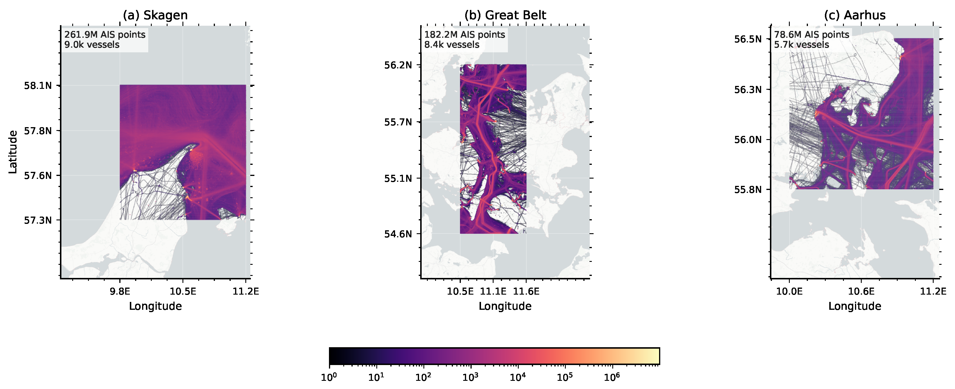
Figure 1 shows the spatial distribution and AIS position density of the three study areas. The density patterns indicate that the three datasets contain both regular sailing routes and locally concentrated vessel movements, making them suitable for evaluating AIS trajectory prediction under different maritime scenarios.

Table 1. Summary of the AIS datasets used in this study.

Dataset	AIS Points	Vessels	Spatial Coverage	Navigational Characteristics
Skagen	261.9 million	9.0k	8.5–$11.3^{\circ }$ E, 57.2–$58.3^{\circ }$ N	Dense traffic junction and route interactions
Great Belt	182.2 million	8.4k	10.2–$11.8^{\circ }$ E, 54.5–$56.4^{\circ }$ N	Constrained waterway and channel effects
Aarhus Bay	78.6 million	5.7k	9.8–$11.2^{\circ }$ E, 55.7–$56.6^{\circ }$ N	Coastal and bay-area vessel movements

summarizes the data scale and spatial coverage of the three AIS datasets. The raw AIS records include timestamp, vessel identifier, longitude, and latitude. The timestamp is used to order vessel movement records, while the vessel identifier is used to separate vessel trajectories and construct leakage-free data splits. For trajectory prediction, vessel positions are represented using local meter-scale two-dimensional coordinates derived from the original longitude and latitude records using the transformation defined in Equation (1).

In addition to the raw AIS data scale,

Table 2. Movement characteristics of trajectory samples under the long-term prediction setting.

Dataset	Inter-Step Distance (km)	Speed (kn)	Heading Change ($°$)
Aarhus Bay	0.073 ± 0.063	7.11 ± 6.16	1.40 ± 6.42
Great Belt	0.047 ± 0.062	4.56 ± 6.07	1.79 ± 8.86
Skagen	0.033 ± 0.079	3.21 ± 7.65	2.65 ± 9.10

reports the movement characteristics of the trajectory samples used for model training and evaluation under the long-term prediction setting. Step distance, vessel speed, and heading change are reported using mean and standard deviation to describe the movement scale, speed variation, and turning intensity of the trajectory samples. These statistics provide a more detailed description of the experimental data distribution and help explain the differences in prediction difficulty among the three regions.

3.2. Experimental Design and Settings

To evaluate the performance of GCT-Former in AIS-based vessel trajectory prediction, all experiments are conducted on the three datasets described above. The use of Skagen, Great Belt, and Aarhus Bay allows the model to be tested under different maritime traffic conditions, including dense route interactions, constrained waterway navigation, and coastal vessel movements. This setting is intended to examine whether the proposed model can maintain stable prediction performance across different spatial patterns and navigation environments.

For each dataset, three prediction horizons are considered to evaluate short-term, medium-term, and long-term forecasting performance. The short-term setting uses 20 historical AIS observations and predicts 20 future positions. The medium-term setting uses the same 20 historical observations but extends the prediction horizon to 40 future positions. The long-term setting uses 40 historical observations to predict 80 future positions. All AIS trajectories are organized at a 20-s temporal interval, so these settings correspond to progressively longer forecasting durations. This design enables the evaluation of both short-range prediction accuracy and long-horizon trajectory stability.

To ensure a fair comparison, all models are trained and evaluated using the same input features, data split, and evaluation metrics. The input of each model consists of local two-dimensional coordinates transformed from the original longitude and latitude records. Before training, the local $x/y$ coordinates are standardized using the mean and standard deviation fitted on the training windows only. The coordinate standardization is formulated as

$${\mathbf{x}}_t^{\mathrm{std}}={\displaystyle \frac{{\mathbf{x}}_t-{\mathit{\mu }}_{\mathrm{train}}}{{\mathit{\sigma }}_{\mathrm{train}}}},$$

(36)

where ${\mathbf{x}}_t={[u_t,v_t]}^{\top }$ denotes the meter-scale local coordinate at time step t, and ${\mathit{\mu }}_{\mathrm{train}}$ and ${\mathit{\sigma }}_{\mathrm{train}}$ are the coordinate-wise mean and standard deviation computed from the training windows. The same normalization parameters are then applied to the validation and test sets. During evaluation, both predicted and ground-truth trajectories are transformed back to the meter-scale local coordinate system by

$${\mathbf{x}}_t={\mathbf{x}}_t^{\mathrm{std}}\odot {\mathit{\sigma }}_{\mathrm{train}}+{\mathit{\mu }}_{\mathrm{train}},$$

(37)

where ⊙ denotes element-wise multiplication. ADE, FDE, RMSE, and MAE are then computed using the inverse-transformed meter-scale coordinates. The datasets are divided into training, validation, and test sets with a ratio of 70%, 10%, and 20%, respectively. The validation set is used for model selection, and the final performance is reported on the test set. Eight representative baseline models are selected for comparison, including MLP [32], Seq2Seq [33], Transformer [34], GRU [35], LSTM [36], BiLSTM [37], PatchTST [38], and DiffTraj [39]. These models cover different trajectory prediction structures, including feed-forward mapping, encoder–decoder prediction, attention-based sequence modeling, recurrent temporal modeling, patch-based time-series Transformer modeling, and diffusion-based trajectory generation. To ensure a fair comparison, all baseline models are implemented and evaluated under the same experimental protocol as GCT-Former, including the same input representation, data split, prediction horizons, and evaluation metrics. Therefore, the performance differences can be primarily attributed to the model architecture rather than differences in data processing or evaluation settings.

3.3. Evaluation Metrics

Let ${\mathbf{y}}_{i,k}\in {\mathbb{R}}^2$ denote the ground-truth future position of the i-th sample at the k-th future step, and let ${\widehat{\mathbf{y}}}_{i,k}\in {\mathbb{R}}^2$ denote the corresponding predicted position. Here, N is the number of test samples and K is the prediction horizon. All distance-based evaluation metrics are computed using the inverse-normalized local coordinates in meters. For reporting, the resulting meter-scale errors are divided by 1000, so the ADE, FDE, RMSE, and MAE values in the result tables are expressed in kilometers. The average displacement error (ADE) is defined as

$$\mathrm{ADE}={\displaystyle \frac{1}{NK}}{\displaystyle \sum _{i=1}^N}{\displaystyle \sum _{k=1}^K}{∥{\widehat{\mathbf{y}}}_{i,k}-{\mathbf{y}}_{i,k}∥}_2.$$

(38)

ADE measures the average spatial deviation between the predicted and ground-truth trajectories over all future steps.

The final displacement error (FDE) is defined as

$$\mathrm{FDE}={\displaystyle \frac{1}{N}}{\displaystyle \sum _{i=1}^N}{∥{\widehat{\mathbf{y}}}_{i,K}-{\mathbf{y}}_{i,K}∥}_2.$$

(39)

FDE measures the prediction error at the final future step and is especially important for evaluating long-horizon trajectory forecasting.

The root mean squared error (RMSE) is calculated as

$$\mathrm{RMSE}=\sqrt{{\displaystyle \frac{1}{NK}}\sum _{i=1}^N\sum _{k=1}^K{∥{\widehat{\mathbf{y}}}_{i,k}-{\mathbf{y}}_{i,k}∥}_2^2}.$$

(40)

RMSE gives larger penalties to relatively large prediction errors.

The mean absolute error (MAE) is defined as

$$\mathrm{MAE}={\displaystyle \frac{1}{NK}}{\displaystyle \sum _{i=1}^N}{\displaystyle \sum _{k=1}^K}{\displaystyle \frac{\left|{\widehat{u}}_{i,k}-u_{i,k}\right|+\left|{\widehat{v}}_{i,k}-v_{i,k}\right|}{2}},$$

(41)

where ${\widehat{\mathbf{y}}}_{i,k}={[{\widehat{u}}_{i,k},{\widehat{v}}_{i,k}]}^{\top }$ and ${\mathbf{y}}_{i,k}={[u_{i,k},v_{i,k}]}^{\top }$. MAE evaluates the average absolute coordinate-wise prediction error. For all metrics, lower values indicate better prediction performance.

4. Results

This section presents the experimental results of GCT-Former on the three AIS trajectory datasets. The results are organized according to the main evaluation objectives of this study. First, the overall prediction performance is compared across different datasets and prediction horizons using ADE, FDE, RMSE, and MAE. Second, an ablation analysis is conducted to examine the contribution of the main architectural components of GCT-Former. Third, the step-wise prediction error is analyzed to show how prediction errors evolve along the forecasting horizon. Finally, the model is evaluated under different maneuvering scenarios, including straight sailing, mild turning, and sharp turning, through both quantitative comparisons and qualitative trajectory examples.

4.1. Overall Prediction Performance

Table 3. Prediction performance comparison in terms of ADE and FDE across different datasets and prediction horizons.

Dataset	Model	Short-Term		Medium-Term		Long-Term
		ADE (km)	FDE (km)	ADE (km)	FDE (km)	ADE (km)	FDE (km)
Aarhus	MLP	0.072	0.156	0.129	0.298	0.372	0.858
	Seq2Seq	0.079	0.173	0.321	0.623	0.686	1.349
	Transformer	0.083	0.161	0.153	0.298	0.479	0.831
	GRU	0.070	0.156	0.129	0.309	0.360	0.837
	LSTM	0.075	0.164	0.124	0.293	0.499	0.887
	BiLSTM	0.075	0.162	0.130	0.303	0.504	0.873
	PatchTST	0.109	0.217	0.181	0.330	0.533	0.997
	DiffTraj	0.085	0.169	0.154	0.310	0.382	0.812
	GCT-Former	0.062	0.141	0.117	0.272	0.344	0.774
Great Belt	MLP	0.045	0.100	0.198	0.475	0.602	1.457
	Seq2Seq	0.050	0.119	0.222	0.530	0.620	1.495
	Transformer	0.057	0.106	0.249	0.530	0.716	1.521
	GRU	0.044	0.100	0.198	0.478	0.587	1.461
	LSTM	0.045	0.101	0.202	0.493	0.601	1.486
	BiLSTM	0.048	0.103	0.218	0.510	1.428	2.459
	PatchTST	0.069	0.110	0.264	0.541	0.757	1.624
	DiffTraj	0.061	0.112	0.228	0.532	0.573	1.414
	GCT-Former	0.041	0.094	0.217	0.526	0.546	1.368
Skagen	MLP	0.025	0.050	0.057	0.147	0.228	0.531
	Seq2Seq	0.033	0.067	0.077	0.164	0.275	0.630
	Transformer	0.039	0.053	0.086	0.134	0.310	0.569
	GRU	0.025	0.050	0.063	0.147	0.261	0.595
	LSTM	0.025	0.052	0.058	0.130	0.237	0.554
	BiLSTM	0.028	0.061	0.058	0.131	0.265	0.595
	PatchTST	0.051	0.067	0.107	0.160	0.330	0.628
	DiffTraj	0.043	0.067	0.092	0.153	0.257	0.560
	GCT-Former	0.023	0.046	0.057	0.130	0.218	0.525

Note: Bold values indicate the best, i.e., lowest, result for each metric under each dataset and prediction horizon. Tied best values after rounding are also shown in bold.

presents the ADE and FDE results across the three datasets and three prediction horizons. ADE and FDE are first reported because they directly describe trajectory-level prediction quality. ADE measures the average spatial deviation over the whole predicted trajectory, while FDE measures the error at the final prediction step, which is particularly important for long-horizon forecasting. Overall, GCT-Former shows strong performance on these core geometric trajectory prediction metrics, especially in the short-term and long-term settings. Starting with the Aarhus dataset, GCT-Former achieves the lowest ADE and FDE under all three prediction horizons. In the short-term setting, it obtains an ADE of 0.062 and an FDE of 0.141. When the prediction horizon is extended to the medium-term setting, GCT-Former maintains the best performance, with an ADE of 0.117 and an FDE of 0.272. In the long-term setting, GCT-Former obtains an ADE of 0.344 and an FDE of 0.774, both of which remain the lowest among all compared models.

A similar trend can be found for Great Belt in the short-term and long-term settings. In the short-term setting, GCT-Former achieves the lowest ADE of 0.041 and the lowest FDE of 0.094. In the long-term setting, it again obtains the best performance, with an ADE of 0.546 and an FDE of 1.368. Nevertheless, the medium-term results show a different pattern. In this setting, MLP and GRU achieve the joint-lowest ADE of 0.198, while MLP obtains the lowest FDE of 0.475. GCT-Former records an ADE of 0.217 and an FDE of 0.526, indicating that the proposed model is not uniformly superior in all medium-term cases. For Skagen, GCT-Former achieves the best or joint-best ADE and FDE across the short-term, medium-term, and long-term settings. In the short-term setting, it obtains an ADE of 0.023 and an FDE of 0.046. In the medium-term setting, it obtains the joint-lowest ADE of 0.057 and the joint-lowest FDE of 0.130. In the long-term setting, GCT-Former achieves an ADE of 0.218 and an FDE of 0.525. Taken together, the ADE and FDE results show that the clearest and most consistent advantage of GCT-Former appears in the long-term setting. Across Aarhus, Great Belt, and Skagen, GCT-Former achieves the best ADE and FDE in all long-term cases.

To further complement the ADE and FDE comparison,

Table 4. Prediction performance comparison in terms of RMSE and MAE across different datasets and prediction horizons.

Dataset	Model	Short-Term		Medium-Term		Long-Term
		RMSE (km)	MAE (km)	RMSE (km)	MAE (km)	RMSE (km)	MAE (km)
Aarhus	MLP	0.151	0.046	0.234	0.084	0.599	0.243
	Seq2Seq	0.173	0.051	0.480	0.218	0.871	0.456
	Transformer	0.154	0.053	0.234	0.099	0.621	0.308
	GRU	0.150	0.045	0.238	0.084	0.596	0.235
	LSTM	0.163	0.048	0.234	0.080	0.693	0.334
	BiLSTM	0.161	0.048	0.239	0.085	0.696	0.334
	PatchTST	0.178	0.071	0.254	0.118	0.682	0.349
	DiffTraj	0.149	0.055	0.241	0.099	0.616	0.247
	GCT-Former	0.143	0.040	0.219	0.075	0.606	0.224
Great Belt	MLP	0.107	0.029	0.464	0.129	1.297	0.391
	Seq2Seq	0.105	0.032	0.505	0.143	1.268	0.401
	Transformer	0.110	0.037	0.547	0.160	1.418	0.464
	GRU	0.108	0.028	0.467	0.128	1.295	0.382
	LSTM	0.109	0.029	0.468	0.131	1.261	0.391
	BiLSTM	0.110	0.031	0.495	0.140	1.992	0.926
	PatchTST	0.111	0.046	0.539	0.169	1.329	0.494
	DiffTraj	0.110	0.038	0.446	0.137	1.206	0.370
	GCT-Former	0.100	0.026	0.565	0.139	1.228	0.351
Skagen	MLP	0.071	0.016	0.185	0.036	0.630	0.144
	Seq2Seq	0.075	0.021	0.186	0.048	0.652	0.176
	Transformer	0.075	0.024	0.188	0.056	0.656	0.196
	GRU	0.070	0.016	0.183	0.040	0.636	0.165
	LSTM	0.069	0.016	0.185	0.037	0.643	0.149
	BiLSTM	0.089	0.018	0.190	0.037	0.674	0.168
	PatchTST	0.084	0.034	0.205	0.071	0.657	0.213
	DiffTraj	0.089	0.027	0.201	0.059	0.624	0.164
	GCT-Former	0.080	0.014	0.187	0.036	0.615	0.137

Note: Bold values indicate the best, i.e., lowest, result for each metric under each dataset and prediction horizon. Tied best values after rounding are also shown in bold.

reports RMSE and MAE across the same datasets and prediction horizons. RMSE emphasizes relatively large deviations, while MAE reflects the average coordinate-wise absolute error. These two metrics provide an additional perspective on the numerical stability of the predicted trajectories. For Aarhus, GCT-Former achieves the lowest RMSE and MAE in both the short-term and medium-term settings. In the short-term setting, the RMSE is 0.143 and the MAE is 0.040. In the medium-term setting, the RMSE is 0.219 and the MAE is 0.075, both of which are the best results among all models. In the long-term setting, GCT-Former obtains the lowest MAE of 0.224 and remains competitive in RMSE with 0.606, while GRU achieves the lowest RMSE of 0.596. The RMSE and MAE results for Great Belt are generally consistent with the ADE and FDE findings. GCT-Former achieves the best RMSE and MAE in the short-term setting, with values of 0.100 and 0.026. In the long-term setting, GCT-Former achieves the lowest MAE of 0.351, while DiffTraj obtains the lowest RMSE of 1.206. However, the medium-term setting again shows weaker performance. In this case, DiffTraj obtains the lowest RMSE of 0.446, while GRU obtains the lowest MAE of 0.128. GCT-Former records an RMSE of 0.565 and an MAE of 0.139. For Skagen, the RMSE and MAE results are more mixed in the short-term and medium-term settings. In short-term prediction, LSTM achieves the lowest RMSE, whereas GCT-Former achieves the lowest MAE. In medium-term prediction, GRU achieves the lowest RMSE, while GCT-Former and MLP obtain the joint-lowest MAE of 0.036. In the long-term setting, however, GCT-Former achieves the best performance on both RMSE and MAE, with values of 0.615 and 0.137. Overall, the combined ADE/FDE and RMSE/MAE results indicate that GCT-Former provides the most consistent advantage in long-term geometric trajectory prediction, particularly in terms of ADE, FDE, and MAE, while some baseline models remain competitive for RMSE and under specific short-term or medium-term metrics.

4.2. Ablation Analysis

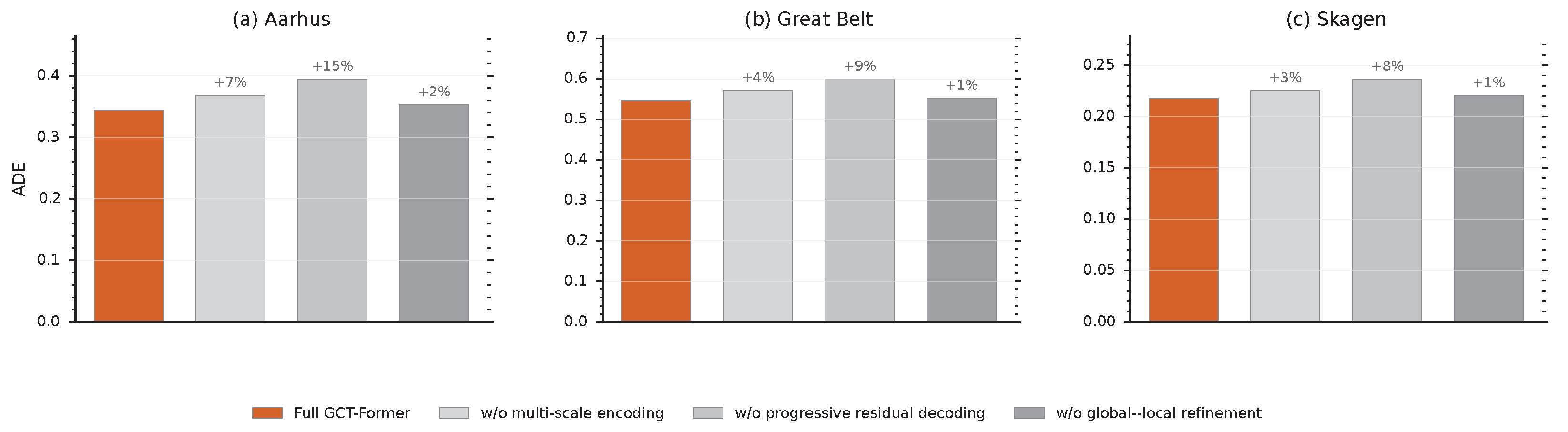
To examine whether the main architectural components of GCT-Former contribute to the final prediction performance, an ablation analysis is conducted under the long-term prediction setting. Figure 2 reports the effect of removing the main components of GCT-Former. The full GCT-Former obtains the lowest ADE on all three datasets. Removing the multi-scale encoding module increases ADE by 7% on Aarhus, 4% on Great Belt, and 3% on Skagen. Removing the progressive residual decoding module leads to a larger degradation, with ADE increasing by 15%, 9%, and 8% on the three datasets, respectively. Removing the global–local refinement module causes a smaller but still observable increase in ADE. These results indicate that all three components contribute to the final performance, with progressive residual decoding showing the most evident contribution to long-horizon prediction.

4.3. Step-Wise Prediction Analysis

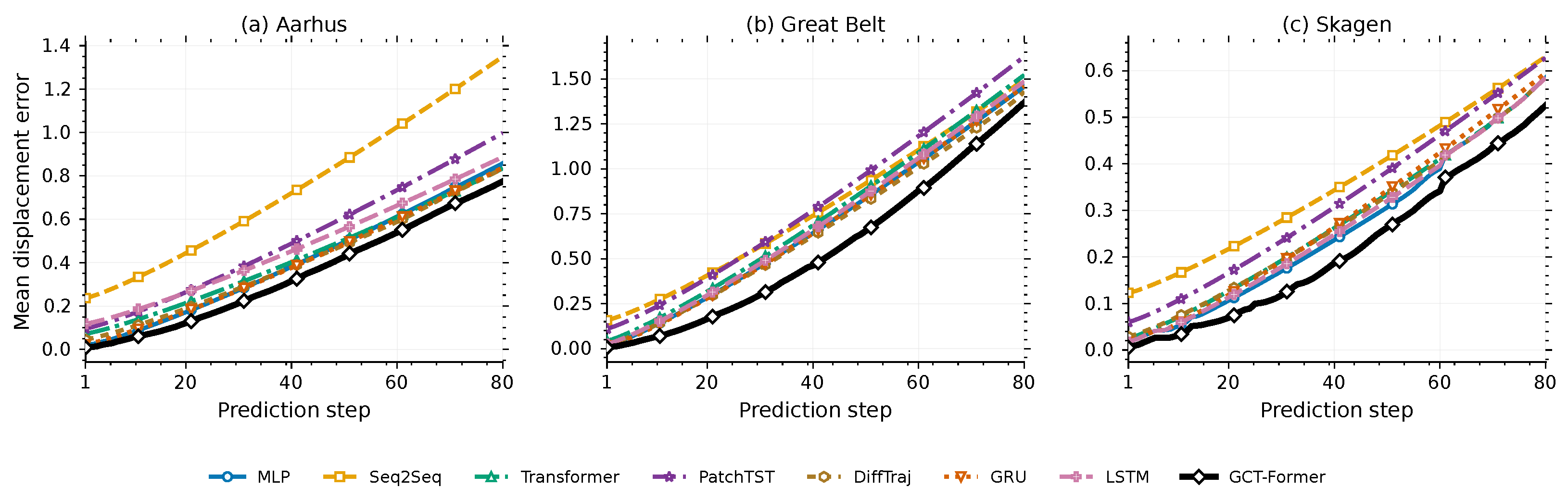
To evaluate how prediction errors accumulate along the forecasting horizon, the step-wise displacement error is analyzed under the long-term prediction setting. Figure 3 shows how the mean displacement error changes as the prediction step increases. Across the three datasets, the error generally increases with the prediction horizon for all models. Compared with the selected baselines, GCT-Former shows a lower and smoother error-growth trend, especially in the later prediction steps. This result is consistent with the ADE and FDE comparisons and suggests that the progressive residual decoding strategy helps reduce error accumulation during long-horizon trajectory generation.

4.4. Maneuvering Scenario Analysis

To evaluate the robustness of GCT-Former under nonlinear vessel movements, the prediction performance is further analyzed under different maneuvering scenarios.

Table 5. Long-term prediction performance under turning maneuvers in terms of ADE and FDE.

Dataset	Model	Mild Turning		Sharp Turning
		ADE (km)	FDE (km)	ADE (km)	FDE (km)
Aarhus	Best baseline	0.449 (MLP)	0.990 (Transformer)	0.526 (GRU)	1.224 (Transformer)
	GCT-Former	0.390	0.765	0.506	1.146
Great Belt	Best baseline	0.338 (GRU)	0.833 (MLP)	1.303 (GRU)	3.190 (Seq2Seq)
	GCT-Former	0.311	0.807	1.216	3.060
Skagen	Best baseline	0.230 (MLP)	0.447 (Transformer)	0.583 (MLP)	1.400 (MLP)
	GCT-Former	0.218	0.433	0.556	1.375

Note: Bold values indicate the lower error between GCT-Former and the best baseline for each metric and maneuvering scenario.

reports the long-term prediction performance under mild-turning and sharp-turning cases. Beginning with Aarhus, GCT-Former outperforms the best baseline under both mild-turning and sharp-turning cases. For mild turning, GCT-Former obtains an ADE of 0.390 and an FDE of 0.765. For sharp turning, it achieves an ADE of 0.506 and an FDE of 1.146. Both results are lower than the corresponding best baseline values. The improvement is also observed on Great Belt. For mild turning, GCT-Former achieves an ADE of 0.311 and an FDE of 0.807. For sharp turning, it obtains an ADE of 1.216 and an FDE of 3.060. Both turning scenarios show lower errors than the corresponding best baselines. Furthermore, Skagen shows the same tendency. Under mild turning, GCT-Former obtains an ADE of 0.218 and an FDE of 0.433. Under sharp turning, it achieves an ADE of 0.556 and an FDE of 1.375.

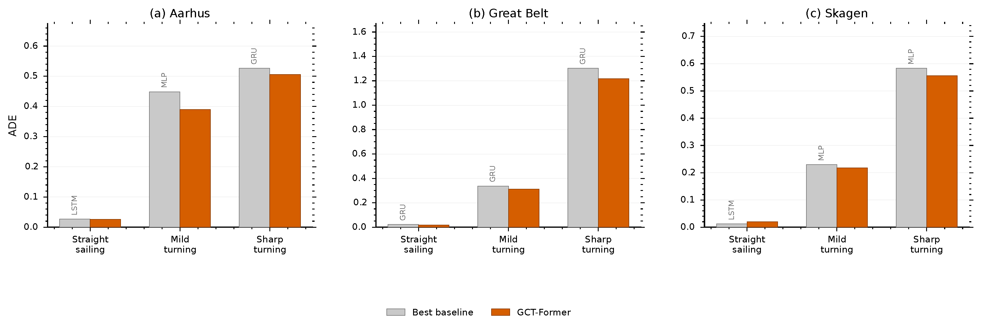
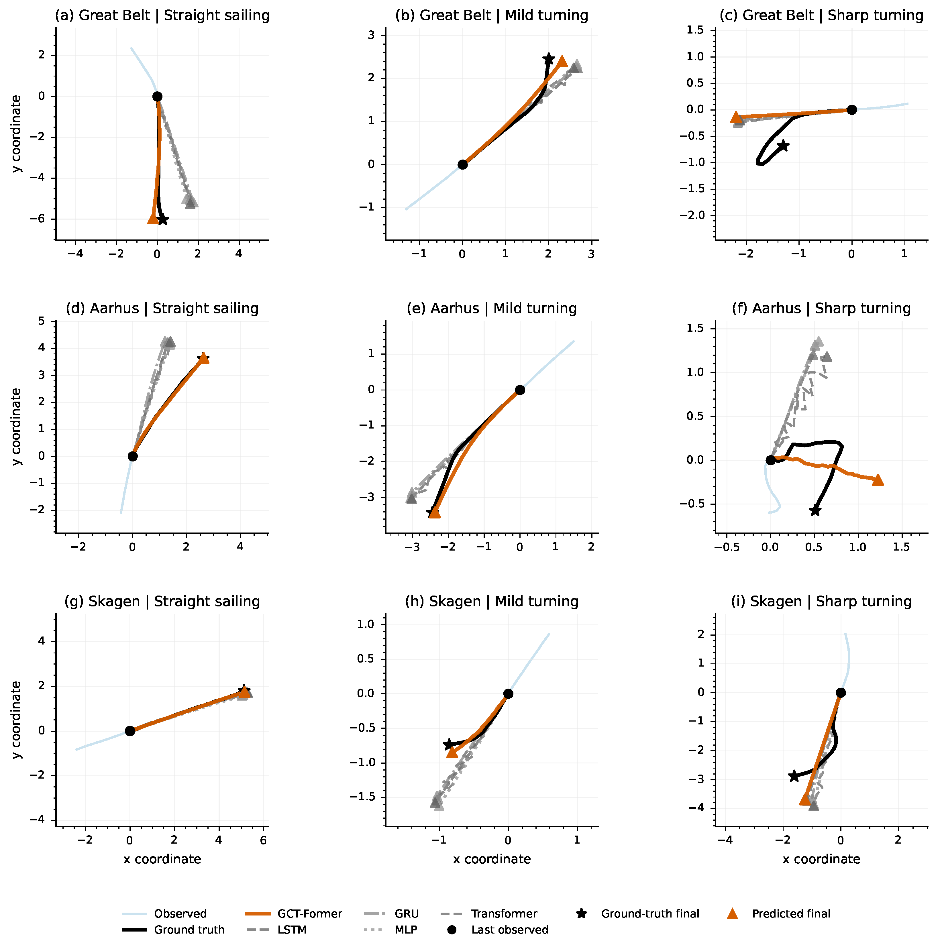
Figure 4 visualizes the ADE comparison under straight-sailing, mild-turning, and sharp-turning scenarios. In the straight-sailing cases, the gap between GCT-Former and the best baseline is relatively small, and GCT-Former is not always the best model. However, under mild-turning and sharp-turning scenarios, GCT-Former consistently shows lower ADE than the corresponding best baseline. This pattern indicates that the advantage of GCT-Former becomes more evident when the maneuvering behavior is more nonlinear.

To provide a visual interpretation of the maneuvering results, representative trajectory examples are further presented in Figure 5. The figure shows long-term trajectory prediction under straight sailing, mild turning, and sharp turning scenarios across the three datasets. It complements the quantitative comparison in Table 5 and Figure 4 by showing how different models behave in terms of trajectory shape, direction, and final-position deviation.

5. Discussion

The experimental results show that GCT-Former is particularly effective for long-horizon AIS trajectory prediction. Combining Table 3 and Table 4, and Figure 3, the proposed model achieves its most consistent advantage in the long-term setting, particularly in terms of ADE, FDE, and MAE, while remaining competitive in RMSE. The step-wise error curves further indicate that GCT-Former can better control error accumulation as the forecasting horizon increases. This result is consistent with the model design: the multi-scale encoder captures historical movement patterns from different temporal ranges, the progressive residual decoder strengthens dependency among future steps, and the global–local refinement module further adjusts the initially decoded trajectory. The ablation results in Figure 2 also support this interpretation, as removing any of the three components increases ADE, with the largest degradation observed when the progressive residual decoding module is removed.

The turning-maneuver results further demonstrate the value of GCT-Former under nonlinear vessel movements. Table 5 and Figure 4 show that GCT-Former achieves lower errors than the corresponding best baseline under mild-turning and sharp-turning scenarios, indicating that the proposed progressive and refinement-based prediction strategy is useful for preserving future trajectory trends when vessel motion becomes nonlinear. The qualitative examples provide similar evidence. In straight-sailing cases, GCT-Former generally follows the ground-truth movement direction with relatively small endpoint deviation. In mild-turning cases, it better captures gradual direction changes, whereas several baselines tend to extend the historical motion trend too linearly. In sharp-turning cases, GCT-Former remains competitive, although extremely high-curvature or loop-like maneuvers are still difficult to reproduce accurately. Despite these advantages, several limitations remain. First, GCT-Former contains multiple components, including the multi-scale encoder, progressive residual decoder, and global–local refinement module. This design improves long-horizon prediction performance but also increases model complexity and may require additional parameter tuning and efficiency analysis before real-time deployment. Second, the current model is a data-driven geometric trajectory prediction framework and does not explicitly incorporate waterway boundaries, navigation rules, environmental conditions, vessel-specific maneuvering constraints, or neighboring-vessel interactions. Third, the prediction performance may be affected by missing AIS records, irregular reporting intervals, position noise, sudden speed changes, and highly irregular maneuvers. These limitations suggest that future work should further investigate model efficiency, data robustness, and the integration of richer maritime-context and risk-assessment information.

6. Conclusions

Accurate vessel trajectory prediction is important for maritime traffic monitoring, navigation safety, route planning, and intelligent vessel traffic management. However, AIS-based trajectory prediction remains challenging because vessel movements are affected by heterogeneous maritime environments, traffic density, channel constraints, and maneuvering behaviors. To address these challenges, this study proposed GCT-Former, a progressive and refinement-based framework for AIS-based vessel trajectory prediction. The proposed model integrates a trajectory-specific multi-scale sequence encoder, a progressive residual decoder, and a global–local trajectory refinement module, enabling it to capture historical movement information from different temporal scales, strengthen the dependency among future prediction steps, and further correct the initially decoded trajectory. Experiments on three Danish AIS datasets, namely Aarhus Bay, Great Belt, and Skagen, show that GCT-Former achieves its most consistent advantage in the long-term prediction setting. In terms of long-term ADE, GCT-Former obtains 0.344, 0.546, and 0.218 on Aarhus Bay, Great Belt, and Skagen, respectively. In terms of long-term FDE, it achieves 0.774, 1.368, and 0.525 on the three datasets, respectively. These results demonstrate that the proposed progressive and refinement-based design is particularly effective for long-horizon AIS trajectory prediction.

The ablation analysis further confirms the contribution of the main model components. Removing the multi-scale encoding module increases long-term ADE by 7%, 4%, and 3% on Aarhus Bay, Great Belt, and Skagen, respectively, while removing the progressive residual decoder causes larger increases of 15%, 9%, and 8%. These results indicate that the progressive residual decoder plays the most important role among the tested components, while the multi-scale encoder and global–local refinement module also contribute to the final prediction performance. The maneuvering-scenario analysis also shows the advantage of GCT-Former under nonlinear vessel movements. Under mild-turning cases, GCT-Former achieves ADE/FDE values of 0.390/0.765, 0.311/0.807, and 0.218/0.433 on Aarhus Bay, Great Belt, and Skagen, respectively. Under sharp-turning cases, it achieves ADE/FDE values of 0.506/1.146, 1.216/3.060, and 0.556/1.375 on the three datasets, respectively. These findings show that GCT-Former can better preserve future trajectory trends when vessel motion becomes nonlinear.

Despite these promising results, several limitations remain. The model contains multiple components, which may increase computational cost and require further efficiency analysis before real-time deployment. Overall, the results show that GCT-Former improves AIS-based geometric trajectory prediction by producing more stable long-horizon future-position estimates and more coherent trajectory shapes under maneuvering scenarios. These predicted trajectories can serve as useful trajectory-level information for downstream maritime traffic monitoring, route planning, and decision-support applications. Future work will further improve the framework from both methodological and application-oriented perspectives. On the methodological side, model efficiency, parameter sensitivity, and robustness to missing or noisy AIS records should be further investigated. On the application side, richer maritime-context information, such as waterway constraints, traffic-flow conditions, vessel-interaction patterns, and navigation-risk indicators, can be incorporated to support closer integration with practical maritime traffic management and decision support.

References

1. Rodrigue, J.P. The geography of maritime ranges: Interfacing global maritime shipping networks with Hinterlands. GeoJournal 2022, 87, 1231–1244. [Google Scholar]
2. Kim, Y.J.; Lee, J.S.; Pititto, A.; Falco, L.; Lee, M.S.; Yoon, K.K.; Cho, I.S. Maritime traffic evaluation using spatial-temporal density analysis based on big AIS data. Appl. Sci. 2022, 12, 11246. [Google Scholar] [CrossRef] [Scilit]
3. Huang, J.C.; Ung, S.T. Risk assessment and traffic behaviour evaluation of ships. J. Mar. Sci. Eng. 2023, 11, 2297. [Google Scholar] [CrossRef] [Scilit]
4. Lv, Z.; Wang, X.; Wang, G.; Xing, X.; Lv, C.; Yu, F. Unmanned surface vessels in marine surveillance and management: Advances in communication, navigation, control, and data-driven research. J. Mar. Sci. Eng. 2025, 13, 969. [Google Scholar] [CrossRef] [Scilit]
5. Troupiotis-Kapeliaris, A.; Kastrisios, C.; Zissis, D. Vessel trajectory data mining: A review. IEEE Access 2025, 13, 4827–4856. [Google Scholar] [CrossRef] [Scilit]
6. Yu, Q.; Yin, X.; Geng, X.; Chen, S.; Yang, J. AISFormer for long-term vessel trajectory prediction. Ocean Eng. 2025, 340, 122098. [Google Scholar] [CrossRef] [Scilit]
7. Han, X.; Zhou, Y.; Weng, J.; Chen, L.; Liu, K. Research on fishing vessel recognition based on vessel behavior characteristics from AIS data. Front. Mar. Sci. 2025, 12, 1547658. [Google Scholar] [CrossRef] [Scilit]
8. Chen, Y.; Chen, Y.; Cui, Y.; Cai, X.; Yin, C.; Cheng, Y. Optimizing vessel trajectories: Advanced denoising and interpolation techniques for AIS data. Ocean Eng. 2025, 327, 120988. [Google Scholar] [CrossRef] [Scilit]
9. Zhang, R.; Fan, Y.; Zhang, D. Research on vessel trajectory fusion method based on extended Kalman filter. In Proceedings of the International Conference on Smart Transportation and City Engineering (STCE 2024); SPIE: Bellingham, WA, USA, 2025; Volume 13575, pp. 48–58. [Google Scholar]
10. Dalsnes, B.R.; Hexeberg, S.; Flåten, A.L.; Eriksen, B.O.H.; Brekke, E.F. The neighbor course distribution method with Gaussian mixture models for AIS-based vessel trajectory prediction. In Proceedings of the 2018 21st International Conference on Information Fusion (FUSION); IEEE: Piscataway, NJ, USA, 2018; pp. 580–587. [Google Scholar]
11. Alizadeh, D.; Alesheikh, A.A.; Sharif, M. Prediction of vessels locations and maritime traffic using similarity measurement of trajectory. Ann. GIS 2021, 27, 151–162. [Google Scholar]
12. Raj, N.; Kumar, P. Navigating the Future: A Comprehensive Review of Vessel Trajectory Prediction Techniques. Def. Sci. J. 2025, 75, 129–138. [Google Scholar] [CrossRef] [Scilit]
13. Li, J.; Wang, X.; Chen, J.; Zhu, D.; Zhang, C.; Chen, Z.; Huang, Y. Ship Trajectory Prediction Method Based on Multi-Layer Recurrent Neural Network Structure and AIS Data Driven. Comput. Intell. 2025, 41, e70079. [Google Scholar]
14. Yin, J.; Yu, Z.; Wu, H. Ship trajectory prediction based on LSTM model with multi-scale convolution and attention mechanism. Ocean Eng. 2025, 338, 122055. [Google Scholar] [CrossRef] [Scilit]
15. Wang, C.; Ren, H.; Li, H. Vessel trajectory prediction based on AIS data and bidirectional GRU. In Proceedings of the 2020 International Conference on Computer Vision, Image and Deep Learning (CVIDL); IEEE: Piscataway, NJ, USA, 2020; pp. 260–264. [Google Scholar]
16. You, L.; Xiao, S.; Peng, Q.; Claramunt, C.; Han, X.; Guan, Z.; Zhang, J. St-seq2seq: A spatio-temporal feature-optimized seq2seq model for short-term vessel trajectory prediction. IEEE Access 2020, 8, 218565–218574. [Google Scholar]
17. Sinni, M.; Kyriazanos, D.M. Vessel Trajectory Prediction Using Robust AIS Preprocessing and Dual-Self-Attention GRU. In Proceedings of the Workshop on AI-Driven Data Engineering and Reusability for Earth and Space Sciences (DARES’25), Co-Located with the 28th European Conference on Artificial Intelligence (ECAI 2025), Bologna, Italy, 25–30 October 2025; pp. 1–10. [Google Scholar]
18. Kim, D.K.; Kim, K. A convolutional transformer model for multivariate time series prediction. IEEE Access 2022, 10, 101319–101329. [Google Scholar] [CrossRef] [Scilit]
19. Nguyen, D.; Fablet, R. A transformer network with sparse augmented data representation and cross entropy loss for ais-based vessel trajectory prediction. IEEE Access 2024, 12, 21596–21609. [Google Scholar] [CrossRef] [Scilit]
20. Wang, W.; Xiong, W.; Ouyang, X.; Chen, L. TPTrans: Vessel trajectory prediction model based on transformer using AIS data. ISPRS Int. J. Geo-Inf. 2024, 13, 400. [Google Scholar] [CrossRef] [Scilit]
21. Chen, X.; Wu, P.; Wu, Y.; Aboud, L.; Postolache, O.; Wang, Z. Ship trajectory prediction via a transformer-based model by considering spatial-temporal dependency. Intell. Robot. 2025, 5, 562–578. [Google Scholar]
22. Er, F.; Yalman, Y. Navigating the Future: A novel PCA-driven layered attention approach for vessel trajectory prediction with encoder–decoder models. Appl. Sci. 2025, 15, 8953. [Google Scholar]
23. Zhao, J.; Yan, Z.; Zhou, Z.; Chen, X.; Wu, B.; Wang, S. A ship trajectory prediction method based on GAT and LSTM. Ocean Eng. 2023, 289, 116159. [Google Scholar] [CrossRef] [Scilit]
24. Feng, H.; Cao, G.; Xu, H.; Ge, S.S. IS-STGCNN: An Improved Social spatial-temporal graph convolutional neural network for ship trajectory prediction. Ocean Eng. 2022, 266, 112960. [Google Scholar]
25. Xiao, Y.; Luo, X.; Wang, T.; Zhang, Z. Spatio-Temporal Transformer Networks for Inland Ship Trajectory Prediction with Practical Deficient Automatic Identification System Data. Appl. Sci. 2024, 14, 10494. [Google Scholar] [CrossRef] [Scilit]
26. Wang, P.; Pan, M.; Liu, Z.; Li, S.; Chen, Y.; Wei, Y. Ship Trajectory Prediction in Complex Waterways Based on Transformer and Social Variational Autoencoder (SocialVAE). J. Mar. Sci. Eng. 2024, 12, 2233. [Google Scholar] [CrossRef] [Scilit]
27. Wu, W.; Yan, D.; Yan, J.; Wang, X. Ship behavior prediction and anomaly detection using LSTM-DCross model based on AIS and remote sensing data. Int. J. Digit. Earth 2025, 18, 2515251. [Google Scholar] [CrossRef] [Scilit]
28. Sanford, C.; Hsu, D.J.; Telgarsky, M. Representational strengths and limitations of transformers. Adv. Neural Inf. Process. Syst. 2023, 36, 36677–36707. [Google Scholar] [CrossRef] [Scilit]
29. Pang, B.; Zha, K.; Cao, H.; Shi, C.; Lu, C. Deep rnn framework for visual sequential applications. In Proceedings of the IEEE/CVF Conference on Computer Vision and Pattern Recognition; IEEE: Piscataway, NJ, USA, 2019; pp. 423–432. [Google Scholar]
30. Chevillon, G. Direct multi-step estimation and forecasting. J. Econ. Surv. 2007, 21, 746–785. [Google Scholar] [CrossRef] [Scilit]
31. Zhou, Y.; Shao, H.; Wang, L.; Waslander, S.L.; Li, H.; Liu, Y. Smartrefine: A scenario-adaptive refinement framework for efficient motion prediction. In Proceedings of the IEEE/CVF Conference on Computer Vision and Pattern Recognition; IEEE: Piscataway, NJ, USA, 2024; pp. 15281–15290. [Google Scholar]
32. Rumelhart, D.E.; Hinton, G.E.; Williams, R.J. Learning representations by back-propagating errors. Nature 1986, 323, 533–536. [Google Scholar] [CrossRef] [Scilit]
33. Sutskever, I.; Vinyals, O.; Le, Q.V. Sequence to Sequence Learning with Neural Networks. In Proceedings of the Advances in Neural Information Processing Systems; Curran Associates, Inc.: Red Hook, NY, USA, 2014; Volume 27. [Google Scholar]
34. Vaswani, A.; Shazeer, N.; Parmar, N.; Uszkoreit, J.; Jones, L.; Gomez, A.N.; Kaiser, L.; Polosukhin, I. Attention Is All You Need. In Proceedings of the Advances in Neural Information Processing Systems; Curran Associates, Inc.: Red Hook, NY, USA, 2017; Volume 30. [Google Scholar]
35. Cho, K.; van Merriënboer, B.; Gulcehre, C.; Bahdanau, D.; Bougares, F.; Schwenk, H.; Bengio, Y. Learning Phrase Representations using RNN Encoder–Decoder for Statistical Machine Translation. In Proceedings of the 2014 Conference on Empirical Methods in Natural Language Processing; ACL: Stroudsburg, PA, USA, 2014; pp. 1724–1734. [Google Scholar]
36. Hochreiter, S.; Schmidhuber, J. Long Short-Term Memory. Neural Comput. 1997, 9, 1735–1780. [Google Scholar] [CrossRef] [Scilit] [PubMed]
37. Schuster, M.; Paliwal, K.K. Bidirectional Recurrent Neural Networks. IEEE Trans. Signal Process. 1997, 45, 2673–2681. [Google Scholar] [CrossRef] [Scilit]
38. Huang, X.; Tang, J.; Shen, Y. Long time series of ocean wave prediction based on PatchTST model. Ocean Eng. 2024, 301, 117572. [Google Scholar] [CrossRef] [Scilit]
39. Zhu, Y.; Ye, Y.; Zhang, S.; Zhao, X.; Yu, J. Difftraj: Generating gps trajectory with diffusion probabilistic model. Adv. Neural Inf. Process. Syst. 2023, 36, 65168–65188. [Google Scholar] [CrossRef] [Scilit]
Figure 1. Spatial distribution and AIS position density of the three study areas: (a) Skagen, (b) Great Belt, and (c) Aarhus Bay.
Jmse 14 01218 g001
Figure 2. Ablation study of GCT-Former components under the long-term prediction setting. The figure reports ADE on Aarhus, Great Belt, and Skagen.
Jmse 14 01218 g002
Figure 3. Step-wise prediction error under the long-term forecasting setting. The figure compares GCT-Former with selected baseline models on Aarhus, Great Belt, and Skagen.
Jmse 14 01218 g003
Figure 4. ADE comparison under different maneuvering scenarios. Each panel compares GCT-Former with the best baseline for straight sailing, mild turning, and sharp turning. The model name above each gray bar indicates the corresponding best baseline.
Jmse 14 01218 g004
Figure 5. Qualitative comparison of long-term trajectory prediction under different maneuvering scenarios.
Jmse 14 01218 g005