Observation-Based Evaluation of Environmental Forcing and Drift Parameterizations for Operational Sargassum Transport Forecasting

Abstract

Since 2011, massive strandings of pelagic Sargassum have become a recurrent environmental hazard across the tropical Atlantic and Caribbean archipelago, creating an urgent need for reliable short-term drift forecasts to support coastal risk management. This study evaluates key sources of uncertainty in operational Sargassum drift forecasting by analyzing the sensitivity of Lagrangian simulations to the representation of floating material and to environmental forcing fields. The analysis uses two complementary observational datasets: trajectories of four GPS-tracked Sargassum mats deployed near Puerto Rico and thirteen 24 h displacement vectors derived from sequential Sentinel-3 satellite detections across the tropical North Atlantic. Drift simulations were performed with the MOTHY model under multiple configurations, testing two material parameterizations, different atmospheric forcings, and several ocean circulation products and vertical current integration strategies. The results indicate that the best agreement with observed trajectories is obtained for partially immersed structures, highlighting the importance of balancing wind exposure and hydrodynamic drag. Sensitivity experiments further show that ocean circulation forcing dominates trajectory skill, while higher-resolution atmospheric forcing provides limited improvement under offshore conditions. Overall, the study confirms the importance of accurately representing upper-ocean transport processes and provides observational support for several operational choices implemented in the Météo-France Sargassum forecasting system.

1. Introduction

Pelagic Sargassum strandings have become, since 2011, a recurrent and large-scale environmental hazard in the northwestern part of the tropical Atlantic and Caribbean regions. The emergence of the so-called Great Atlantic Sargassum Belt has led to unprecedented biomass transport across the tropical Atlantic toward the Caribbean Sea and the Gulf of Mexico [1,2]. While offshore Sargassum mats provide important ecological services by offering habitat and trophic support to diverse pelagic communities [3], their massive accumulation nearshore generates severe environmental, sanitary, and socio-economic impacts. Once stranded, decomposing algae release toxic gases such as hydrogen sulfide and ammonia and modify the physical and chemical properties of surrounding waters, affecting human health and coastal ecosystems, and strongly impacting tourism and fisheries-dependent economies [4,5].

The need to anticipate coastal Sargassum strandings has stimulated the rapid development of monitoring and forecasting systems combining satellite remote sensing and numerical modeling. Recent syntheses have reviewed the state of knowledge on Sargassum ecology, detection techniques, transport modeling, and growth processes in the tropical Atlantic [6,7]. In parallel, a comprehensive assessment of operational monitoring and forecasting systems has highlighted both methodological diversity and persistent scientific gaps, particularly concerning the integration of transport dynamics and biological processes across scales [8].

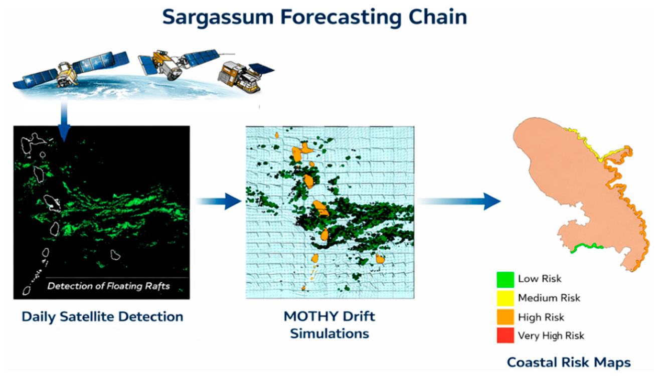
To support French public authorities confronted with these chronic Sargassum crises, in 2019, Météo-France implemented an operational forecasting service dedicated to predicting Sargassum stranding risk in the French Antilles and French Guiana [9]. The system combines daily satellite detection of floating rafts, Lagrangian drift simulations, and expert interpretation to produce short-term coastal Sargassum stranding bulletins (Figure 1).

Satellite observations are first processed using ocean-color radiometry and spectral indices designed to detect floating Sargassum, such as the Maximum Chlorophyll Index (MCI) [10] and the Alternative Floating Algae Index (AFAI) [11]. These detections are then used to initialize particle-based simulations performed with an adapted version of the MOTHY (Oceanic Model for Transport of HYdrocarbons) Météo-France transport model. The model is forced by operational atmospheric winds and ocean circulation fields, and provides 4-day trajectory forecasts. The operational objective is probabilistic rather than deterministic, aiming to estimate the likelihood and potential intensity of coastal impacts rather than predicting exact beaching locations.

Despite significant progress in basin-scale monitoring and seasonal outlook systems [12,13,14], several limitations remain in short-term drift forecasting. As emphasized by Debue et al. [6], uncertainties affect both detection and modeling stages, including nearshore satellite retrieval constraints, simplified growth parameterizations, and incomplete representation of vertical and sub-mesoscale dynamics. Likewise, Putman et al. [8] underline that forecasting skill critically depends on how transport processes are represented and how atmospheric and oceanic forcings are integrated.

The parameterization of partially submerged and deformable macroalgal rafts remains poorly constrained by dedicated observations. In particular, the effective windage and depth of interaction with the upper ocean are not well characterized for Sargassum aggregations. Moreover, Dagestad and Röhrs [15] emphasize that uncertainties in ocean current fields generally represent the dominant source of error in ocean trajectory forecasting, often exceeding those associated with atmospheric forcing. These limitations underline the need for observation-based evaluation of drift parameterizations in operational contexts.

The present study focuses specifically on the exploitation of two complementary observational datasets: four in situ drifter trajectories and thirteen satellite-derived drift sequences. Rather than addressing the full forecasting chain, the analysis concentrates on the drift modeling component. These observational datasets are used to evaluate how the MOTHY operational model represents floating Sargassum, to assess the relative contribution of atmospheric and oceanic forcings in trajectory simulations.

By confronting model outputs with observed drift pathways, this work contributes to strengthening the physical basis of operational Sargassum transport forecasting, in line with the needs for improved validation and process understanding identified in recent reviews [6,7,8].

2. Materials and Methods

This study investigates the main sources of uncertainty affecting operational Sargassum drift forecasting through the combined use of two independent validation datasets. The first dataset consists of GPS-tracked drifters deployed southwest of Puerto Rico and described by Putman et al. [16], including instruments embedded directly within natural Sargassum rafts. The second dataset comprises 24 h displacement trajectories derived from sequential satellite detections of Sargassum over a broad region extending on either side of the Lesser Antilles. Both datasets were selected to study the drift of Sargassum rafts in the Caribbean region.

The joint use of these datasets provides complementary constraints on model performance. The instrumented drifters offer controlled in situ Lagrangian trajectories, enabling detailed evaluation of structural representation and short-term transport dynamics. In contrast, the satellite-derived cases reflect realistic basin-scale operational conditions, capturing the variability and complexities encountered in routine forecasting. Together, they allow a robust assessment of model sensitivity across both controlled experimental and operational environments.

2.1. Observational Datasets

2.1.1. Putman Sargassum Drifter Dataset

The observational dataset used for model validation originates from the drifting buoy experiments described in Putman et al. [16]. In this study, SPOT Trace GPS trackers were affixed directly to natural mats of Sargassum located approximately 11 km off the southeast coast of Puerto Rico. By embedding the devices within floating algae aggregates, the recorded positions provide in situ measurements of authentic Sargassum raft motion under realistic environmental forcing conditions.

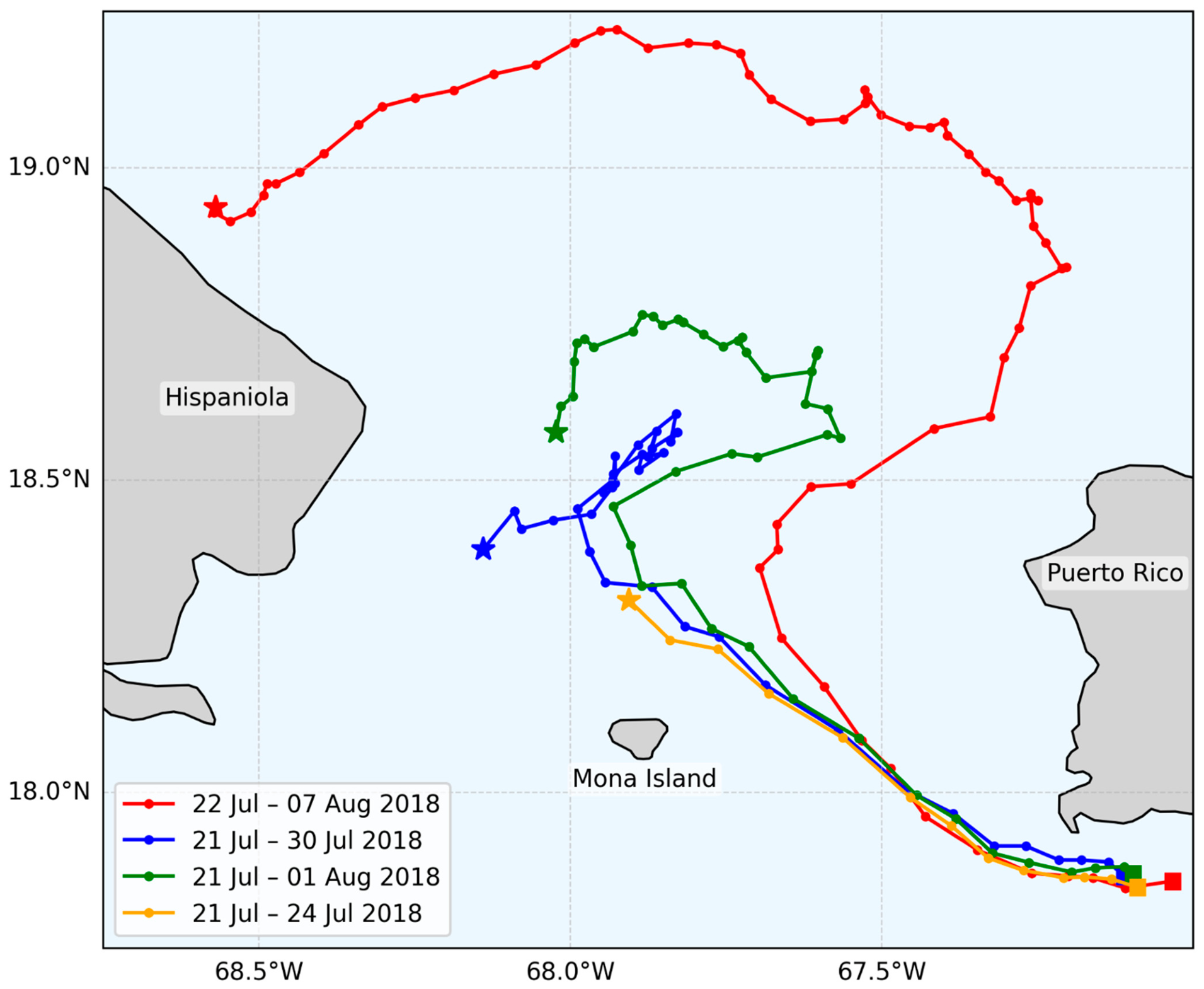
Location data were transmitted via the Globalstar satellite system at approximately 6 h intervals. Individual Sargassum mats were tracked for periods ranging from 6 to 21 days, with the overall observational campaign spanning from 8 June 2018 to 23 August 2018 (Figure 2).

Overall, the trajectories of the four buoys were analyzed over successive 24 h periods, representing a cumulative total of 39 days of observations. These data, collected in the Caribbean Sea, provides a robust basis for evaluating the performance of the MOTHY model in this region closed to the French Antilles.

2.1.2. Satellite-Derived 24 h Drift Dataset

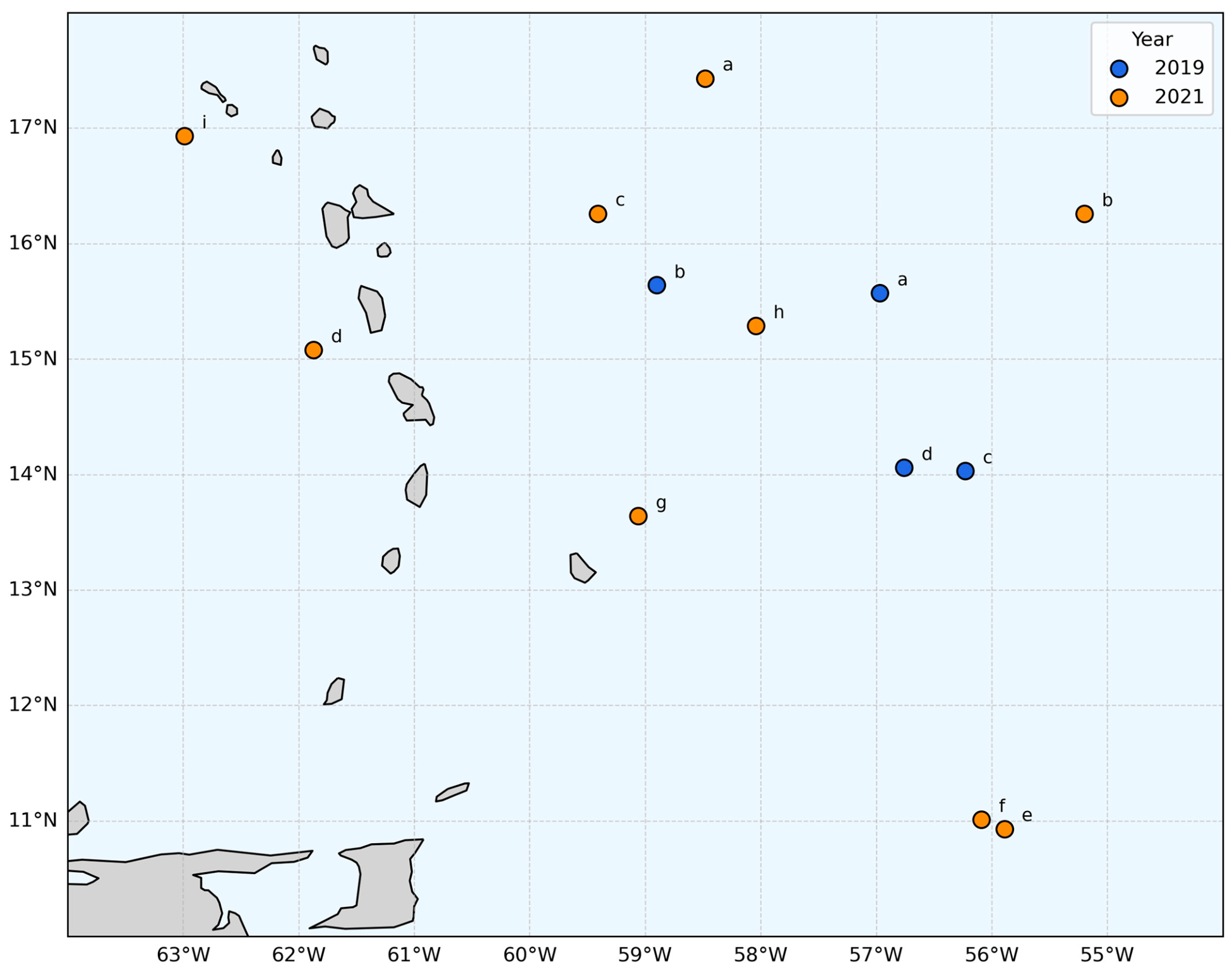
A set of 13 independent Sargassum drift events was selected from sequential satellite observations. Each case corresponds to a clearly identifiable and isolated raft carefully tracked over a 24 h period, between two satellite tracks, in the tropical North Atlantic off the coast of the Caribbean arc. The rafts were subjectively identified in 2019 and 2021 by visual inspection of remote sensing images acquired by the Ocean and Land Color Instrument (OLCI) onboard the Sentinel-3A and Sentinel-3B satellites, using the Earth Observation (EO) Browser platform [17]. The positions of the tracked rafts are shown in

Table 1. Coordinates of satellite-detected Sargassum rafts positions in the tropical North Atlantic in 2019 and 2021. Day 1 (resp. Day 2) corresponds to the satellite’s first pass (resp. the following pass, at approximately the same time the following day) of the drift tracking.

Rafts	Day 1	Latitude 1	Longitude 1	Day 2	Latitude 2	Longitude 2
a	13 May 2019	15.57	−56.97	14 May 2019	15.68	−57.00
b	13 May 2019	15.64	−58.90	14 May 2019	15.49	−59.03
c	14 May 2019	14.03	−56.23	15 May 2019	14.00	−56.28
d	14 May 2019	14.06	−56.76	15 May 2019	14.12	−56.90
a	1 November 2021	17.43	−58.48	2 November 2021	17.42	−58.54
b	1 November 2021	16.26	−55.20	2 November 2021	16.21	−55.43
c	12 November 2021	16.26	−59.41	13 November 2021	16.25	−59.56
d	15 July 2021	15.08	−61.87	16 July 2021	15.15	−61.93
e	16 July 2021	10.93	−55.89	17 July 2021	11.09	−55.97
f	16 July 2021	11.01	−56.00	17 July 2021	11.08	−56.10
g	16 July 2021	13.64	−59.06	17 July 2021	13.49	−59.06
h	4 June 2021	15.29	−58.04	5 June 2021	15.26	−58.02
i	3 May 2021	16.93	−62.99	4 May 2021	17.04	−63.12

and Figure 3.

Rafts were selected based on their relatively small size and spatial isolation in order to minimize ambiguity in feature continuity between successive images.

The use of short-duration trajectories (24 h) was constrained by the temporal sampling of the satellite observations, as the study area is typically revisited only once per day.

For each selected case, the initial geographic coordinates of the raft’s center were extracted at time t₀ and the final coordinates at time t₀ + 24 h. Situations affected by significant cloud cover or uncertain raft identification were excluded from the analysis.

The resulting set of 24 h displacement vectors, compiled in 2019 and 2021, constitutes the operational-scale validation dataset used to evaluate model performance under realistic basin-scale forecasting conditions.

2.2. Drift Modeling Framework

The MOTHY marine drift model, developed by Météo-France, was originally designed to simulate oil spill trajectories [18]. It was subsequently extended to drifting containers [19] and later adapted for search and rescue (SAR) applications. When the operational Sargassum forecasting chain was implemented in 2019, the hydrocarbon configuration was selected as the most suitable framework for representing Sargassum rafts. This choice was motivated by its ability to account for horizontal dispersion and, importantly, to simulate particle trajectories within the upper few meters below the sea surface, thereby better reproducing the observed drift behavior of Sargassum. To ensure that particles remain within this near-surface layer, a density of 1020 kg·m⁻³ was prescribed, closely approximating the density of seawater (1026 kg·m⁻³) and allowing the simulated material to evolve just beneath the surface.

Ocean currents are explicitly resolved through the hydrodynamic module embedded within MOTHY. This module combines a two-dimensional shallow-water formulation with a one-dimensional eddy-viscosity scheme [18] and is supplemented by currents from operational ocean circulation models that represent the large-scale background flow. To prevent double counting of wind forcing, already accounted for in the MOTHY hydrodynamic module, the background current is extracted at the base of the Ekman layer [20]. This configuration has proven to be the most effective both over continental shelves [18] and in deep-water environments [21]. In equatorial regions, the background current is computed as the mean velocity over the upper 100 m of the water column. This methodology was validated during a dedicated field exercise conducted off the coast of French Guiana in 2021 [22].

2.3. Representation of Floating Material

Two modeling approaches were evaluated within MOTHY to represent floating material.

The first approach uses the hydrocarbon mode, originally developed for oil spill simulations [18]. In this configuration, floating material is represented by a set of 1000 numerical particles advected by ocean currents and affected by turbulent diffusion and buoyancy processes. Unlike the container mode described below, these particles do not represent discrete physical objects but numerical tracers whose transport properties are controlled by their density and vertical behavior within the water column.

Vertical particle motion follows the original MOTHY parameterization described by Daniel [18]. Each particle is assigned a diameter randomly distributed between 300 and 1200 µm. At each model time step, vertical displacement results from the combined effects of turbulent vertical diffusion and buoyancy. The stochastic diffusion term accounts for turbulent mixing within the upper ocean, while buoyancy depends on particle diameter, particle density, seawater density, and viscosity. As a consequence, particles with a density close to the seawater density undergo repeated vertical excursions controlled by the competition between weak buoyancy and turbulent mixing.

In the operational Sargassum forecasting configuration, a density of 1020 kg·m⁻³ is prescribed, close to seawater density (approximately 1026 kg·m⁻³). Under these conditions, particles oscillate within the upper few meters of the water column rather than remaining permanently at the surface. Because wind influence decreases with depth, these particles experience weaker effective wind forcing and therefore drift more slowly than lighter particles remaining closer to the surface.

In the absence of a universally established density value for floating Sargassum, a density of 250 kg·m⁻³ was also tested in the MOTHY simulations. This value corresponds to reported estimates of fresh wet Sargassum biomass density used in volume-to-mass conversion approaches for coastal accumulation assessments. In particular, Devault et al. [23] adopted an average density of 250 kg·m⁻³ to convert volume estimates derived from airborne data into mass when assessing large-scale influxes of Sargassum in the Caribbean. Although the precise water content of stranded or floating Sargassum can vary depending on drainage time, compaction, and environmental conditions, the value of 250 kg·m⁻³ lies within the range commonly assumed for freshly accumulated, uncompressed biomass. It therefore represents a realistic and literature-supported bulk density for testing sensitivity in transport and accumulation modeling with MOTHY.

To represent the cohesive structure of Sargassum rafts, a second approach based on the container mode was also tested. In this configuration, floating objects are represented as rectangular cuboids with immersion rates ranging from 50% to 100% (in 10% increments) and 7 different heights: 5 cm, 10 cm, 50 cm, 100 cm, 243 cm, 400 cm and 600 cm where 243 cm is the typical height of a container and default height in MOTHY. This range was selected to encompass the variability reported for pelagic Sargassum rafts, from thin surface mats only a few centimeters thick to more typical aggregations of approximately 10–50 cm, and up to multi-meter accumulations occasionally observed in situ (up to about 7 m) [24].

In this formulation, windage is explicitly applied to the emerged fraction of the object, allowing the aerodynamic drag associated with partial emergence to be directly represented. Such a representation may be physically consistent with the behavior of Sargassum rafts, which can behave as semi-submerged floating bodies subject to non-negligible wind forcing. Several observational and modeling studies have shown that including a wind-dependent velocity component can improve the simulation of Sargassum drift, highlighting the importance of direct wind momentum transfer to the exposed biomass [25,26,27]. In this context, the container parameterization implemented in MOTHY [19] may provide a suitable framework for representing windage effects on cohesive Sargassum aggregations within a Lagrangian modeling approach.

The intercomparison was performed using the Putman Sargassum drifter dataset. All combinations of immersion rates and container heights were tested, together with the two density values considered in the hydrocarbon mode. These simulations were performed over a cumulative period of 39 days, resulting in a total of 1716 numerical experiments.

2.4. MOTHY Forcing Products

2.4.1. Atmospheric Forcing Products

Wind forcing is a primary driver of surface drift through direct wind drag and wave-induced processes. Two operational numerical weather prediction systems were evaluated: the global European Centre for Medium-Range Weather Forecasts (ECMWF) Integrated Forecasting System (IFS) and the regional Météo-France AROME Antilles configuration.

The IFS is a global spectral numerical weather prediction system providing dynamically consistent atmospheric fields at synoptic to planetary scales [28]. The operational configuration used here operates at a horizontal resolution of 1/10°, then interpolated to 1/8° for the MOTHY model, with hourly temporal resolution. Its advanced data assimilation scheme and globally balanced dynamics ensure physically coherent wind forcing, making IFS particularly suitable for basin-scale drift simulations and offshore applications, and fully consistent with global ocean circulation products such as GLO12, which is forced by IFS at the surface.

In contrast, the AROME Antilles model is a non-hydrostatic mesoscale atmospheric model developed by Météo-France [29]. It operates at convection-permitting resolution 1/40° with hourly temporal resolution. It explicitly resolves small-scale atmospheric structures such as coastal jets, gust fronts, and orographically induced flows.

Due to its fine spatial resolution, AROME is expected to better capture nearshore wind variability and coastal wind intensification effects. Testing AROME against IFS allows assessment of the importance of high-resolution atmospheric forcing in coastal drift simulations.

The comparison between IFS and AROME therefore isolates the sensitivity of trajectory calculations to wind resolution.

2.4.2. Ocean Forcing Products

Accurate representation of ocean surface currents is essential for drift simulations, as surface advection largely controls transport pathways over time scales of a few days. In order to assess the sensitivity of simulated trajectories to oceanic forcing, three hydrodynamic products with contrasting spatial resolutions, dynamical frameworks, and operational objectives were considered: GLO12, SMOC and CAR36.

The Copernicus Marine global ocean configuration GLO12 [30] corresponds to the operational global analysis and forecast system currently implemented in the Sargassum forecasting chain. It provides daily analyses and forecasts at a horizontal resolution of 1/12° (~9 km). As a data-assimilative, eddy-permitting global system, GLO12 delivers dynamically consistent circulation fields constrained by satellite and in situ observations, making it particularly suitable for offshore and basin-scale applications.

SMOC (Surface Merged Ocean Current) is a dedicated surface current product derived from GLO12 that integrates additional wave-induced (Stokes drift) and tidal current components into the background Eulerian circulation [30,31]. The use of SMOC allows evaluation of whether a single, fully merged surface current product could replace the traditional combination of background circulation and wind-induced drift within the operational framework.

At the regional scale, the CAR36 configuration is a high-resolution Caribbean model with a horizontal grid spacing of 1/36° (~3 km) [32]. Its finer resolution allows improved representation of mesoscale eddies, narrow boundary currents, and complex island-induced flow patterns characteristic of the Caribbean arc. CAR36 is therefore particularly relevant for resolving regional circulation features that may significantly influence drift pathways, especially in coastal and archipelagic environments.

For methodological consistency, the intercomparison was performed using daily surface current products only.

2.4.3. Integration Strategies for Ocean Products

In addition to the wind-driven current internally computed by the MOTHY drift model, a background ocean circulation is introduced to account for geostrophic and large-scale dynamical contributions not explicitly resolved by the wind module. Three vertical integration strategies were tested in order to evaluate the sensitivity of simulated trajectories to the depth at which the background current is extracted.

• Currents at the Base of the Ekman Layer

The first approach consists of integrating the background current at the base of the Ekman layer. This configuration is currently implemented in the operational Sargassum forecasting chain for latitudes above 12° N. The Ekman depth is computed theoretically from the surface wind stress derived from the IFS atmospheric forcing, ensuring dynamical consistency between wind forcing and the depth of the wind-driven layer.

Below the Ekman layer, currents are assumed to represent the geostrophic and large-scale circulation components that supplement the wind-induced drift already calculated by MOTHY. In the study region, which lies sufficiently far from the equator, the Ekman approximation remains dynamically relevant. To date, Mercator Ocean International provides Météo-France with subsurface currents from GLO12 and CAR36 corresponding to this Ekman-base formulation.

• Vertically Averaged Currents over 0–100 m

The second approach consists of using currents vertically averaged over the upper 100 m of the water column. This strategy is implemented operationally for latitudes below 12° N, where the classical Ekman theory becomes less valid due to the weakening of the Coriolis parameter near the equator. As the Coriolis force approaches zero, the theoretical Ekman spiral structure breaks down, and defining a physically meaningful Ekman depth becomes problematic.

In such equatorial or near-equatorial environments, the 0–100 m averaged current provides a robust alternative representation of the upper-ocean transport, capturing both wind-driven and geostrophic components integrated over the mixed layer and thermocline interface.

Although the study area is located sufficiently far from the equator for the Ekman-base approach to remain theoretically applicable, the 0–100 m averaged currents were also examined. This comparison allows assessment of whether the vertically averaged formulation yields comparable or improved drift skill in the region and helps identify the most relevant integration mode for operational purposes.

• Surface Currents Only (SMOC Configuration)

A third configuration was tested using the SMOC (Surface Merged Ocean Current) product, which directly provides total surface currents including background circulation, tidal components, and wave-induced Stokes drift. In this setup, the hydrodynamic module of MOTHY is disabled, and the SMOC surface current is used as the sole ocean forcing.

This configuration enables evaluation of whether a fully merged surface product can replace the traditional formulation combining MOTHY-computed wind drift with a subsurface background current. It therefore provides insight into the relative importance of vertical integration choices versus direct use of a comprehensive surface current product.

The 13 drift cases from the satellite-derived dataset, each with a 24 h duration in the same geographical area, were analyzed under the different forcing configurations, resulting in a total of 73 simulations.

Table 2. List of the tested configurations.

Year	Atmospheric Forcing	Ocean Forcing	Method of Integration	Model Mode	Number of Drift Cases
2018	IFS	GLO12	Base Ekman layer	Hydrocarbon and container	1716
2021	IFS	SMOC	Surface	Hydrocarbon mode	9
2019 and 2021	IFS	GLO12	Base Ekman layer	Hydrocarbon mode	13
2019 and 2021	IFS	GLO12	Averaged over 100 m	Hydrocarbon mode	13
2019 and 2021	IFS	CAR36	Base Ekman layer	Hydrocarbon mode	13
2019 and 2021	IFS	CAR36	Averaged over 100 m	Hydrocarbon mode	13
2019	IFS	GLO12	Surface	Hydrocarbon mode	4
2019	AROME	CAR36	Base Ekman layer	Hydrocarbon mode	4
2019	AROME	CAR36	Averaged over 100 m	Hydrocarbon mode	4

. shows the different tested configurations.

2.5. Model Validation Metrics

Model performance was evaluated using quantitative Lagrangian validation metrics in order to identify the most appropriate forcing configuration and parameter set. For each simulation, a skill score was calculated following the methodology proposed by Liu and Weisberg [33] and subsequently applied in operational drift evaluation frameworks [34].

This skill score is based on the cumulative separation distance between simulated and observed trajectories, normalized by the total length of the observed trajectory:

$$s ={\displaystyle \frac{{\sum }_{i=1}^N{d}_i}{{\sum }_{i=1}^N{l}_{oi}}}$$

(1)

where s represents the normalized cumulative separation distance, N is the total number of time steps i, dᵢ denotes the distance between the modeled and observed positions at time step i, and l_oi corresponds to the length of the observed trajectory at time step i.

The skill score (ss) is then derived from s as follows:

$$ss =\{\begin{array}{cc}1-s/n& s \le n\\ 0& s > n\end{array}$$

(2)

where n denotes the tolerance threshold applied to the model.

The tolerance threshold represents the distance scale used to normalize the trajectory error and defines the strictness of the comparison between modeled and observed trajectories. In this study, a threshold index equal to 1 was adopted. The resulting metric ranges from 0 to 1: values close to 1 indicate a very good agreement between modeled and observed trajectories, whereas values approaching 0 indicate poor predictive performance. A skill score under 0.5 already reflects the difficulty of reproducing observed trajectories.

3. Results

3.1. Representations of Floating Material

Two configurations of the MOTHY model: the hydrocarbon mode and the container mode, were evaluated using the Putman Sargassum drifter dataset. Wind forcing was provided by IFS, while ocean currents were extracted from GLO12 at the base of the Ekman layer. Other configurations, particularly those based on AROME and CAR36, are not available for this region.

For each of the 1716 numerical experiments, the distance between the observed and modeled trajectories after 24 h was computed and used to derive the corresponding skill scores.

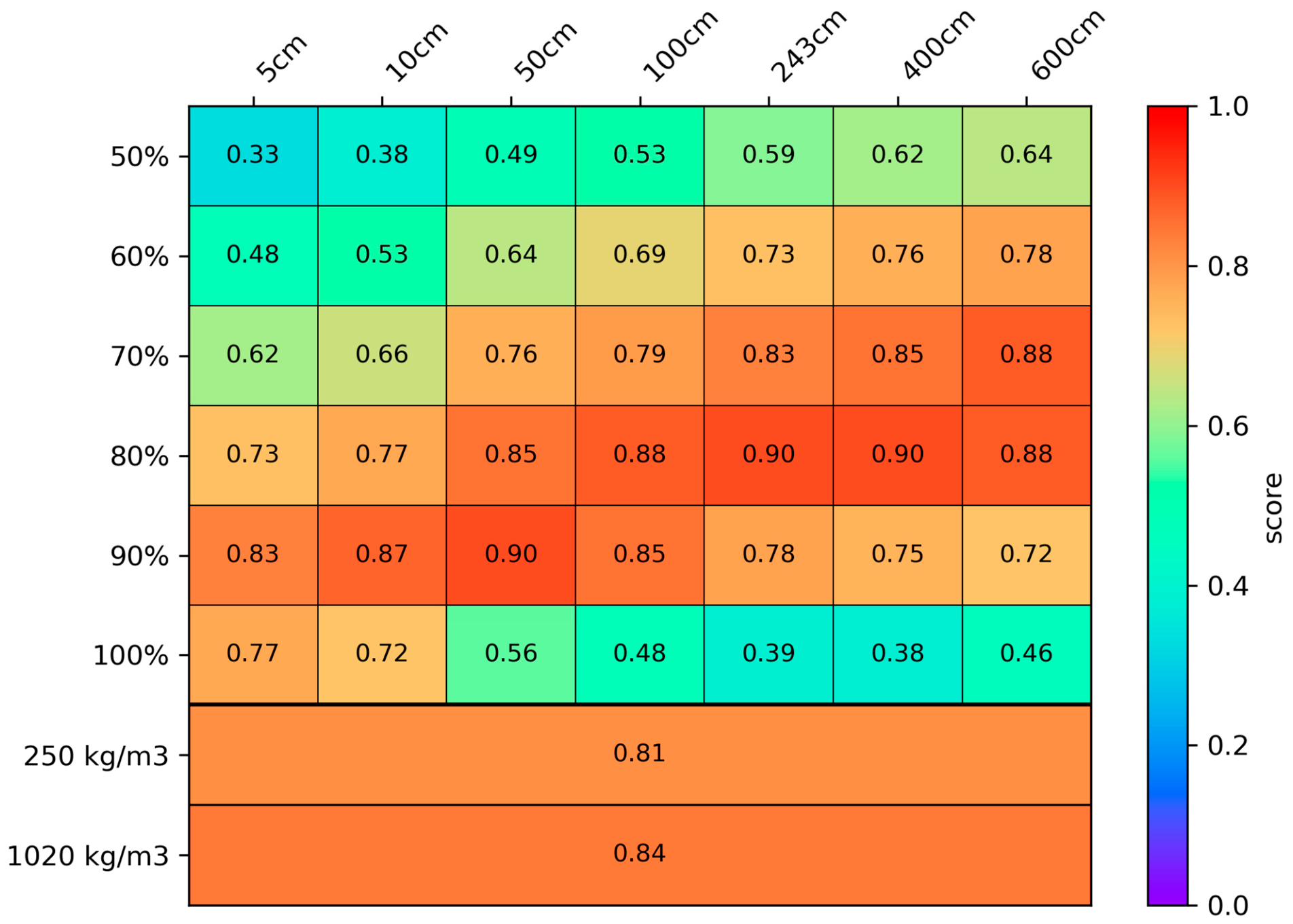
Figure 4 shows the Liu–Weisberg skill scores after the first 24 h of drift for different combinations of container immersion (50–100%) and characteristic vertical extent (5–600 cm). Two additional rows correspond to simulations performed in the hydrocarbon mode, with particle densities of 250 kg·m⁻³ and 1020 kg·m⁻³.

The sensitivity analysis highlights the importance of the balance between wind exposure and submerged drag. Fully immersed configurations (100%) are not directly affected by wind forcing and therefore drift too slowly relative to the observed Sargassum mats, resulting in low skill scores. Conversely, weakly immersed structures (50–70%) are more strongly exposed to the wind, leading to drift speeds that are generally too high. The highest skill scores (≈0.9) are obtained for intermediate immersion levels (80–90%), which provide the most realistic balance between direct wind forcing on the emerged structure and hydrodynamic drag on the submerged portion.

In the hydrocarbon mode, particles with a density of 250 kg·m⁻³ remain at the surface and therefore experience stronger wind forcing, resulting in faster drift. In contrast, particles with a density of 1020 kg·m⁻³ oscillate between the surface and several meters depth, where the influence of the wind is weaker, leading to slower drift and slightly higher skill scores.

The environmental conditions encountered during the drift period also influence model performance. During the first 24 h, immediately southwest of Puerto Rico, the mats drifted within a relatively steady current regime under persistent winds of about 15 knots. In the following days, the trajectories entered regions characterized by more variable winds, currents, and complex bathymetry, where atmospheric and oceanic forcings are likely represented with lower accuracy.

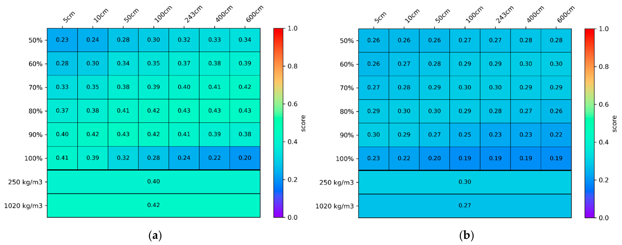
Figure 5 summarizes the results when the 24 h simulations are evaluated over the entire observation period, corresponding to 39 cumulative days of drift for the four mats. Figure 5a presents the mean skill score, while Figure 5b shows the standard deviation, reflecting the variability of model performance over time.

Compared with the first-day analysis (Figure 4), the mean skill scores decrease, generally ranging from 0.20 to 0.43 depending on the parameter configuration. This reduction reflects the increasing difficulty of reproducing observed trajectories under more variable environmental conditions. Nevertheless, the main patterns identified in the short-term analysis remain visible: configurations with 80–90% immersion still provide the best agreement with observations, with mean scores around 0.42–0.43, particularly for intermediate vertical extents (50–243 cm). Fully immersed configurations continue to perform poorly, especially for large vertical extents, confirming that simulations without direct wind forcing underestimate the drift speed of Sargassum mats.

The hydrocarbon-mode simulations yield mean skill scores of 0.40 for particles with a density of 250 kg·m⁻³ and 0.42 for 1020 kg·m⁻³, values comparable to the best-performing container configurations. As in the 24 h analysis, surface particles experience stronger wind forcing, whereas denser particles that oscillate below the surface drift slightly more slowly and show marginally improved agreement with the observations.

Figure 5b also reveals substantial variability in skill scores, with standard deviations typically ranging between 0.19 and 0.30. This variability reflects the changing environmental conditions encountered along the trajectories and the sensitivity of simulated drift to fluctuations in wind and current forcing. Overall, the results indicate that partially immersed configurations provide the most realistic representation of Sargassum drift, while also highlighting the limitations associated with environmental variability and forcing uncertainties.

3.2. Evaluation of Drift Simulations Using Satellite-Derived Trajectories

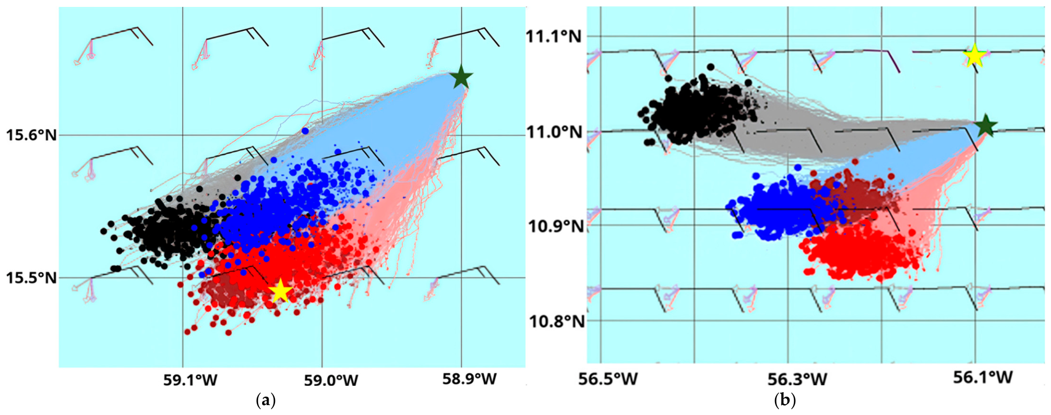
The results of MOTHY simulations, listed in Table 2., reveal two distinct categories of drift behavior. In six of the thirteen cases, the modeled trajectories evolve in a direction broadly consistent with the observed drift from the initial release point, suggesting that the model is able to represent the dominant large-scale transport patterns controlling the displacement of the rafts (Figure 6a). In contrast, in the remaining cases the simulated trajectories diverge substantially from the observed direction, resulting in zero skill scores and indicating limited predictive skill for these particular events (Figure 6b).

The relatively large proportion of unsuccessful simulations (7 out of 13 cases, corresponding to 54% of the dataset) deserves particular attention. Rather than indicating systematic deficiencies in the drift model itself, these discrepancies likely reflect the combined effects of several sources of uncertainty affecting both the observational dataset and the environmental forcing fields.

A first source of uncertainty concerns the ocean circulation products used to force the simulations. The analyzed Sargassum rafts were located in a region characterized by energetic mesoscale and submesoscale variability associated with eddies, filaments, frontal structures, and tropical instability waves. Such structures can locally modify current direction and magnitude over spatial scales of only a few kilometers and time scales shorter than one day. Although the GLO12 and CAR36 products provide high-resolution operational ocean currents, a significant fraction of this small-scale variability remains unresolved or only partially represented. Because the observed trajectories correspond to relatively short 24 h displacements, even small errors in the representation of local circulation structures may produce substantial trajectory divergence.

A second source of uncertainty arises from the methodology used to construct the observational dataset itself. The drift vectors were reconstructed by visually identifying an apparently isolated Sargassum raft in successive Sentinel-3 images separated by approximately 24 h. Although particular care was taken to select isolated rafts with similar shape and size, the identification process cannot guarantee with complete certainty that the same aggregation was tracked on both images. Between two satellite overpasses, floating Sargassum structures may fragment, merge with nearby patches, or undergo rapid morphological changes caused by convergence zones and wave action. In some cases, the observed final position may therefore correspond to a different or structurally modified aggregation.

An additional limitation results from the temporal sampling of the observations. The use of only two positions separated by 24 h provides a highly constrained validation framework, since no intermediate positions are available to reconstruct the actual trajectory followed by the raft. Consequently, the apparent displacement vector only represents the net displacement between two observations, while potentially complex intermediate trajectory changes remain unknown.

To better interpret the results, it is important to distinguish between absolute trajectory prediction skill and relative sensitivity between forcing configurations. The primary objective of this experiment is not to demonstrate perfect deterministic prediction of individual Sargassum raft trajectories, which remains extremely challenging under operational conditions, but rather to evaluate the relative influence of different forcing products and transport parameterizations under realistic forecasting conditions.

For this reason, only cases showing non-zero skill scores were retained for the sensitivity analysis presented in the following Section 3.3. Restricting the comparison to cases where the dominant transport direction is reasonably reproduced allows a more robust evaluation of the relative contribution of atmospheric forcing, ocean circulation products, and vertical integration strategies. The seven unsuccessful cases nevertheless highlight an important limitation of current operational Sargassum forecasting systems and emphasize the need for improved observational datasets with higher temporal resolution and better characterization of short-scale ocean variability.

3.3. Sensitivity to Environmental Forcing

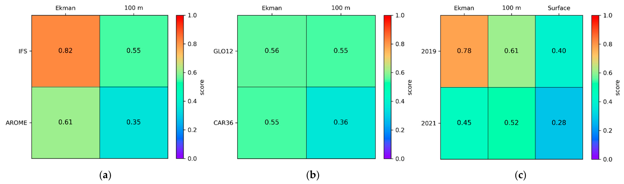
Because the configuration using atmospheric forcing from AROME was only available with the CAR36 ocean configuration in 2019, the comparison between atmospheric forcings is restricted to that year. The results indicate that simulations forced by IFS systematically produce higher skill scores than those forced by AROME, regardless of the ocean current integration method (Figure 7a). When the ocean current is taken either at the base of the Ekman layer or averaged over the upper 100 m, IFS yields scores of 0.82 and 0.55, respectively, compared with 0.61 and 0.35 for AROME. This difference likely reflects the spatial context of the analyzed drifts: the considered Sargassum rafts are located far from the islands, where the higher spatial resolution of AROME does not significantly improve the representation of atmospheric forcing. In such offshore conditions, the large-scale forcing provided by IFS appears sufficient and even slightly more consistent with the observed drift.

A second sensitivity analysis compares the impact of ocean forcing, using GLO12 and CAR36, combined with the two integration methods (Ekman base vs. 100 m average) (Figure 7b). The resulting skill scores are very similar between configurations. GLO12 produces slightly higher values (0.56 vs. 0.55 at the Ekman base and 0.55 vs. 0.36 at 100 m), but these differences remain small and are not statistically significant. This limited sensitivity is again consistent with the offshore location of the Sargassum rafts, where mesoscale coastal dynamics resolved by the higher-resolution CAR36 configuration play a reduced role. Regarding the integration method, using the current at the base of the Ekman layer tends to provide slightly better scores than averaging currents over the upper 100 m, particularly for the CAR36 configuration. Although the improvement is modest and not systematic for GLO12, this result supports the operational choice of using the Ekman-layer base current in the drift modeling chain.

Finally, the performance of simulations based on surface products was evaluated (Figure 7c). These experiments use ocean surface currents for 2019 and SMOC currents for 2021. In both cases, the resulting skill scores are significantly lower than those obtained when using subsurface-integrated currents. For instance, the surface current configuration yields score of 0.40 in 2019 and 0.28 in 2021, compared with 0.61–0.78 when using Ekman-layer or 100 m-integrated currents. This degradation indicates that surface products alone do not adequately represent the effective transport experienced by floating Sargassum rafts. The results therefore confirm that integrating currents within the upper ocean layer, rather than relying solely on surface currents, provides a more realistic representation of drift dynamics in the study region.

4. Discussion

The present study evaluates the sensitivity of short-term Sargassum drift simulations to the representation of floating material and to environmental forcing fields by confronting model trajectories with two complementary observational datasets: GPS-tracked Sargassum mats and satellite-derived displacement vectors. Although limited in number, these observations provide valuable constraints for assessing the realism of drift parameterizations and the operational choices implemented in the forecasting chain. The results highlight the importance of representing the partially submerged nature of Sargassum rafts, while also emphasizing the dominant role of ocean circulation in determining short-term transport pathways. At the same time, the analysis illustrates the current limitations associated with the scarcity of observational datasets and the challenges involved in validating drift models for floating Sargassum.

4.1. Representation of Floating Sargassum

One of the primary objectives of this work was to assess how the physical representation of floating material influences simulated drift trajectories. Two modeling approaches were evaluated to represent floating Sargassum within the MOTHY framework: the container mode and the hydrocarbon mode. The container formulation explicitly represents partially emerged floating bodies by separating aerodynamic drag acting on the emerged fraction from hydrodynamic resistance applied to the submerged portion. From a physical perspective, this formulation is therefore well suited to represent cohesive Sargassum rafts behaving as semi-submerged structures.

However, despite this conceptual advantage, the comparison between both approaches shows that the container and hydrocarbon modes produce similar skill scores in the drift simulations. Because the hydrocarbon configuration allows particles to oscillate within the upper meters of the water column, it indirectly reproduces the combined influence of wind forcing and near-surface currents on floating material. However, the MOTHY drift model represents Sargassum rafts only as independent particles (in hydrocarbon mode) or as blocks (in container mode) and does not consider elasticity, biological interactions or biogeochemical process that may influence their dynamics.

For operational purposes, the hydrocarbon mode was ultimately retained in the forecasting system. Beyond providing comparable trajectory skill, this configuration offers two important advantages for operational Sargassum monitoring. First, it enables the representation of horizontal dispersion processes affecting floating material during transport. Second, it allows the number of released particles to be directly linked to the intensity of the satellite detection index used to identify Sargassum aggregations. This capability makes it possible to represent not only the drift pathways but also the relative amount of Sargassum detected by satellite observations. The hydrocarbon formulation therefore provides a practical framework for coupling satellite-derived detection products with Lagrangian drift simulations in an operational forecasting context.

Overall, these results indicate that while several parameterizations can reproduce the main characteristics of Sargassum drift, operational implementations must balance physical realism with practical considerations related to data assimilation, dispersion representation, and integration with satellite observations.

4.2. Influence of Ocean Circulation and Current Integration

Beyond the representation of floating material, the accuracy of drift simulations strongly depends on the quality of environmental forcing fields. Among these forcings, ocean circulation plays a dominant role in controlling transport pathways. The sensitivity experiments conducted with different ocean products show relatively small differences between the global GLO12 configuration and the higher-resolution regional CAR36 model. This result is likely related to the offshore location of most analyzed drift cases, where the large-scale circulation patterns are already adequately represented by global ocean models.

Previous studies have similarly identified ocean current uncertainties as one of the primary sources of error in Lagrangian trajectory simulations [15]. In the present study, the divergence observed in several satellite-derived drift cases likely reflects the combined effects of unresolved mesoscale and sub-mesoscale processes that cannot be fully captured by the available circulation products.

A key aspect of the modeling framework concerns the method used to integrate ocean currents within the upper water column. The results indicate that simulations using currents extracted at the base of the Ekman layer generally produce slightly higher skill scores than those based on currents averaged over the upper 100 m. Although the differences remain modest, this finding supports the operational choice adopted in the forecasting chain, where the Ekman-based current is used to represent the background circulation beneath the wind-driven layer in non-equatorial region.

Within the MOTHY framework, the drift of floating material is partly governed by a hydrodynamic parameterization that implicitly accounts for the effect of wind forcing on the upper ocean layer and on partially submerged objects [18]. This formulation effectively represents wind-induced drift and its interaction with near-surface circulation. When simulations rely solely on surface-current products, such as direct surface velocities or merged datasets like SMOC [31], this parameterization is not applied. Although SMOC includes additional components such as tidal currents and wave-induced Stokes drift, it does not reproduce the combined effect of wind forcing and near-surface vertical structure represented in the MOTHY configuration.

As a consequence, using surface currents alone is not sufficient to properly represent the drift of partially submerged Sargassum rafts within this modeling framework. The resulting trajectories tend to deviate more strongly from observations, leading to lower skill scores. These results therefore confirm that, in the context of the MOTHY system, combining the internally computed wind-driven drift with subsurface ocean circulation provides a more consistent and realistic representation of Sargassum transport than relying solely on externally provided surface-current products.

4.3. Atmospheric Forcing and Offshore Drift Conditions

The comparison between atmospheric forcing products indicates that the global IFS winds generally produce slightly higher skill scores than the higher-resolution AROME configuration. This result may appear unexpected, given the finer spatial resolution of the mesoscale model. However, even though the various atmospheric and oceanic conditions over the study area are likely not all considered, the analyzed drift events occur mostly in offshore environments, far from complex coastal topography where high-resolution atmospheric models typically provide the greatest benefit.

In such open-ocean conditions, the large-scale wind structures represented by global numerical weather prediction systems are generally sufficient to capture the dominant atmospheric forcing acting on floating material. The limited improvement obtained with higher-resolution winds suggests that, in the studied region, ocean circulation uncertainties may have a larger influence on drift simulations than atmospheric forcing resolution. Similar conclusions have been reported in operational drift modeling studies, where the accuracy of ocean current fields often dominates the forecast skill of trajectory simulations [15].

4.4. Limitations of Observational Datasets

A major challenge in evaluating Sargassum drift models lies in the scarcity of available observational datasets. The present analysis relies on only four GPS-tracked Sargassum mats and thirteen satellite-derived drift cases. While these datasets represent valuable benchmarks, they remain extremely limited and somewhat dated compared to the needs of robust model validation.

The relatively high proportion of unsuccessful short-term trajectory reconstructions observed in the satellite-derived dataset (54% of cases) illustrates the intrinsic difficulty of validating Sargassum drift models using sparse satellite observations alone. It suggests that part of the apparent model error may originate from observational uncertainty rather than deficiencies in the transport parameterization itself. This limitation should be considered when interpreting the relatively low predictive skill obtained for some of the analyzed cases.

The difficulty in acquiring such observations is largely related to the nature of pelagic Sargassum aggregations. Floating rafts are highly dynamic, spatially dispersed, and often transient. Deploying instruments within natural rafts is logistically challenging, and satellite observations are frequently affected by cloud cover and limited revisit frequency. As highlighted in recent reviews of Sargassum monitoring and forecasting systems, the lack of in situ measurements remains a major limitation for improving model validation and understanding transport processes [6,7,8].

Satellite-based tracking also presents intrinsic limitations. Satellites used for Sargassum detection operate on sun-synchronous polar orbits, resulting in revisit intervals that are typically close to one day for a given location. This temporal sampling often prevents continuous tracking of individual rafts. Between successive satellite passes, rafts may fragment, merge, or move outside the detection area, introducing uncertainties in the identification of the same aggregation over time. In addition, the cloud mask can hide Sargassum rafts.

4.5. Emerging Observational Initiatives

The limited number of observations used in this study, and their age, highlights the current scarcity of in situ measurements available for validating Sargassum drift simulations and emphasizes the need for expanded observational efforts. Recognizing this limitation, several recent initiatives aim to strengthen the integration of in situ measurements, satellite observations, and modeling approaches. In addition to the drifter experiments used in this study [16], complementary field campaigns have deployed GPS trackers directly within natural Sargassum aggregations in order to monitor the displacement of individual mats. For example, Fidai et al. [35] embedded low-cost GPS trackers within Sargassum mats in the Caribbean Sea, enabling continuous tracking of floating aggregations and providing valuable in situ observations of drift pathways. Similar approaches are also being implemented within the SargAlert project [36], which aims to significantly improve forecasts of Sargassum strandings across the tropical Atlantic, the Caribbean Sea, and the Brazilian coast by combining satellite observations, transport modeling, artificial intelligence methods, and dedicated in situ measurements.

Complementary observational efforts also include airborne measurements. In spring 2025, a dedicated campaign conducted off the coast of Guadeloupe acquired high-resolution validation data for both detection algorithms and drift modeling using drone flyovers equipped with a multispectral camera [37]. These observations provide detailed information on raft morphology, spatial distribution, and short-term displacement of Sargassum aggregations. Such datasets are particularly valuable because they support both the validation of satellite detection products and the improvement of transport model parameterizations.

Taken together, these new observational initiatives will help provide valuable reference datasets to complement the model validation and sensitivity analyses conducted in this study.

4.6. Perspectives for Improved Satellite Monitoring and Forecasting

Recent developments in satellite observation capabilities offer promising opportunities to improve the monitoring of Sargassum drift. A major limitation of current detection systems is their relatively low temporal resolution, since polar-orbit sensors typically revisit a given region only once per day, which restricts the reconstruction of continuous drift trajectories.

Geostationary satellites may partially overcome this limitation. Instruments such as the Advanced Baseline Imager (ABI) onboard GOES (Geostationary Operational Environmental Satellite) [38] and the Flexible Combined Imager (FCI) onboard Meteosat Third Generation (MTG) provide observations at high temporal frequency, typically every 10–15 min. However, individual images are often affected by noise, cloud contamination, low spatial resolution and atmospheric effects, which limits their direct use for Sargassum detection. In practice, temporal aggregation over several hours is generally required to obtain reliable signals. Despite this constraint, the resulting effective temporal resolution remains significantly higher than the 24 h revisit interval of polar-orbit satellites, offering improved capability to monitor short-term Sargassum displacement.

The combined use of geostationary and polar-orbit satellite observations could therefore contribute to a more comprehensive monitoring system to improve the performance of operational Sargassum forecasting systems [39].

5. Conclusions

This study evaluated key sources of uncertainty affecting short-term Sargassum drift simulations by examining the sensitivity of Lagrangian trajectories to both the representation of floating material and the environmental forcing fields used in operational forecasting. The analysis combined two complementary observational datasets, GPS-tracked Sargassum mats and satellite-derived drift trajectories, providing empirical constraints for assessing the realism of drift model configurations.

Results highlight the importance of representing the partially submerged nature of Sargassum rafts, as the balance between wind exposure and hydrodynamic drag strongly influences simulated drift speeds. While the container parameterization offers a physically explicit representation of semi-emergent floating structures, the hydrocarbon configuration implemented in the MOTHY model provides comparable predictive skill while maintaining advantages for operational applications, particularly in terms of particle dispersion and integration with satellite-derived detection indices.

Preliminary sensitivity experiments investigating atmospheric and oceanic forcing, as well as their implementation within the MOTHY drift model, have been carried out. The results are consistent with the current configuration used in the Météo-France operational Sargassum forecasting system. However, the limited availability of in situ observations remains a significant constraint for robust model validation, and these findings will need to be confirmed using more consistent and comprehensive datasets. Future efforts should therefore focus on expanding observational datasets through coordinated drifter deployments and improved satellite tracking techniques, which could substantially enhance the accuracy and reliability of operational Sargassum drift forecasting in the tropical Atlantic.

References

1. Wang, M.; Hu, C.; Barnes, B.B.; Mitchum, G.; Lapointe, B.; Montoya, J.P. The great Atlantic Sargassum belt. Science 2019, 365, 83–87. [Google Scholar] [CrossRef]
2. Johns, E.M.; Lumpkin, R.; Putman, N.F.; Smith, R.H.; Muller-Karger, F.E.; Rueda-Roa, D.T.; Hu, C.; Wang, M.; Brooks, M.T.; Gramer, L.J.; et al. The establishment of a pelagic Sargassum population in the tropical Atlantic: Biological consequences of a basin-scale long distance dispersal event. Prog. Oceanogr. 2020, 182, 102269. [Google Scholar] [CrossRef]
3. Monroy-Velázquez, L.V.; Canizales-Flores, H.M.; Camacho-Cruz, K.A.; Corbin, M.; Briones-Fourzán, P.; van Tussenbroek, B.I. Faunal associations of holopelagic Sargassum spp. in the subtropical and tropical northern Atlantic: A review. Harmful Algae 2025, 149, 102961. [Google Scholar] [CrossRef] [PubMed]
4. Rodríguez-Martínez, R.E.; Torres-Conde, E.G.; Rosellón-Druker, J.; Cabanillas-Terán, N.; Jáuregui-Haza, U. The Great Atlantic Sargassum Belt: Impacts on the Central and Western Caribbean-A review. Harmful Algae 2025, 144, 102838. [Google Scholar] [CrossRef] [PubMed]
5. Resiere, D.; Florentin, J.; Névière, R. Evaluating the ten-year health impact of hydrogen sulfide (H2S) and ammonia (NH3) exposure from sargassum seaweed invasions in the Caribbean: Public health implications. Harmful Algae 2026, 152, 103027. [Google Scholar] [CrossRef] [PubMed]
6. Debue, M.; Guinaldo, T.; Jouanno, J.; Chami, M.; Barbier, S.; Berline, L.; Chevalier, C.; Daniel, P.; Daniel, W.; Descloitres, J.; et al. Understanding the Sargassum phenomenon in the Tropical Atlantic Ocean: From satellite monitoring to stranding forecast. Mar. Pollut. Bull. 2025, 216, 117923. [Google Scholar] [CrossRef] [PubMed]
7. Hu, C.; Barnes, B.B.; Qi, L.; Gower, J.F.R.; Jiao, J.; Xie, Y. Monitoring pelagic Sargassum in the Atlantic Ocean from space: Principles and practices. Harmful Algae 2025, 144, 102840. [Google Scholar] [CrossRef] [PubMed]
8. Putman, N.F.; Beyea, R.T.; Ackerman, E.G.; Trinanes, J.; Le Hénaff, M.; Hu, C.; Lumpkin, R. Systems to monitor and forecast pelagic Sargassum inundation of coastal areas across the North Atlantic: Present tools and future needs. Harmful Algae 2025, 149, 102933. [Google Scholar] [CrossRef] [PubMed]
9. Debue, M.; Guinaldo, T.; Ayache, D.; Bacheviller, F.; Barbier, S.; Berthomier, L.; Blot, E.; Conseil, S.; Daniel, P.; Daniel, W.; et al. Prévision des échouements de sargasses aux Antilles françaises. La Météorol. 2025, 131, 53–60. [Google Scholar] [CrossRef]
10. Gower, J.; Hu, C.; Borstad, G.; King, S. Ocean color satellites show extensive lines of floating Sargassum in the Gulf of Mexico. IEEE Trans. Geosci. Remote Sens. 2006, 43, 361–366. [Google Scholar] [CrossRef]
11. Wang, M.; Hu, C. Mapping and quantifying Sargassum distribution and coverage in the Central West Atlantic using MODIS observations. Remote Sens. Environ. 2016, 183, 350–367. [Google Scholar] [CrossRef]
12. Wang, M.; Hu, C. Predicting Sargassum blooms in the Caribbean Sea from MODIS observations. Geophys. Res. Lett. 2017, 44, 3265–3273. [Google Scholar] [CrossRef]
13. Marsh, R.; Oxenford, H.A.; Cox, S.-A.L.; Johnson, D.R.; Bellamy, J. Forecasting seasonal sargassum events across the tropical Atlantic: Overview and challenges. Front. Mar. Sci. 2022, 9, 914501. [Google Scholar] [CrossRef]
14. Jouanno, J.; Morvan, G.; Berline, L.; Benshila, R.; Aumont, O.; Sheinbaum, J.; Ménard, F. Skillful Seasonal Forecast of Sargassum Proliferation in the Tropical Atlantic. Geophys. Res. Lett. 2023, 50, e2023GL105545. [Google Scholar] [CrossRef]
15. Dagestad, K.-F.; Röhrs, J. Prediction of ocean surface trajectories using satellite derived vs. modeled ocean currents. Remote Sens. Environ. 2019, 223, 130–142. [Google Scholar] [CrossRef]
16. Putman, N.F.; Lumpkin, R.; Olascoaga, M.J.; Trinanes, J.; Goni, G.J. Improving transport predictions of pelagic Sargassum. J. Exp. Mar. Biol. Ecol. 2020, 529, 151398. [Google Scholar] [CrossRef]
17. Sentinel Hub EO Browser. Available online: https://apps.sentinel-hub.com/eo-browser/ (accessed on 9 March 2026).
18. Daniel, P. Operational forecasting of oil spill drift at Météo-France. Spill Sci. Technol. Bull. 1996, 3, 53–64. [Google Scholar] [CrossRef]
19. Daniel, P.; Jan, G.; Cabioc’h, F.; Landau, Y.; Loiseau, E. Drift modeling of cargo containers. Spill Sci. Technol. Bull. 2002, 7, 279–288. [Google Scholar] [CrossRef]
20. Law-Chune, S. Apport de L’océanographie Opérationnelle à L’amélioration de la Prévision de Dérive Océanique dans le Cadre D’opérations de Recherche et de Sauvetage en mer et de Lutte Contre les Pollutions Marines. Ph.D. Thesis, University of Toulouse III, Toulouse, France, 2012. [Google Scholar]
21. Daniel, P.; Paradis, D.; Gouriou, V.; Le Roux, A.; Garreau, P.; Le Roux, J.-F.; Louazel, S. Forecast of oil slick drift from Ulysse/CSL Virginia and Grande America accidents. Proc. Int. Oil Spill Conf. 2021, 2021, 1141410. [Google Scholar]
22. Martin, S.; Gouriou, V. Étude Comparative des Modèles de Prévision de Dérive et de Comportements des Hydrocarbures; Technical Report R.21.35.C/3401; Cedre: Brest, France, 2021; Available online: https://doc.cedre.fr/index.php?lvl=notice_display&id=10572 (accessed on 17 June 2026).
23. Devault, D.A.; Modestin, E.; Cottereau, V.; Vedie, F.; Stiger-Pouvreau, V.; Pierre, R.; Le Bouchard, F.; Mora, P. The Silent Spring of Sargassum. Environ. Sci. Pollut. Res. 2021, 28, 15580–15583. [Google Scholar] [CrossRef] [PubMed]
24. Ody, A.; Thibaut, T.; Berline, L.; Ménard, F.; Talbot, V.; Le Gendre, R.; Gramer, L.J.; Aumont, O.; Dumas, F.; Lapointe, B.E.; et al. From In Situ to satellite observations of pelagic Sargassum distribution and aggregation in the Tropical North Atlantic Ocean. PLoS ONE 2019, 14, e0222584. [Google Scholar] [CrossRef] [PubMed]
25. Putman, N.F.; Goni, G.J.; Gramer, L.J.; Hu, C.; Johns, E.M.; Triñanes, J.; Wang, M. Simulating transport pathways of pelagic Sargassum from the Equatorial Atlantic into the Caribbean Sea. Prog. Oceanogr. 2018, 165, 205–214. [Google Scholar] [CrossRef]
26. Marsh, R.; Addo, K.A.; Jayson-Quashigah, P.-N.; Oxenford, H.A.; Maxam, A.; Anderson, R.; Skliris, N.; Dash, J.; Tompkins, E.L. Seasonal predictions of holopelagic Sargassum across the tropical Atlantic accounting for uncertainty in drivers and processes: The SARTRAC ensemble forecast system. Front. Mar. Sci. 2021, 8, 722524. [Google Scholar] [CrossRef]
27. Podlejski, W.; Berline, L.; Nerini, D.; Doglioli, A.; Lett, C. A new Sargassum drift model derived from features tracking in MODIS images. Mar. Pollut. Bull. 2023, 188, 114629. [Google Scholar] [CrossRef] [PubMed]
28. ECMWF: IFS Documentation—Cy46r1, Operational Implementation, Part IV: Physical Processes. 2019. Available online: https://www.ecmwf.int/en/elibrary/81141-ifs-documentation-cy46r1-part-iv-physical-processes (accessed on 17 June 2026). [CrossRef]
29. Seity, Y.; Brousseau, P.; Malardel, S.; Hello, G.; Bénard, P.; Bouttier, F.; Lac, C.; Masson, V. The AROME-France convective-scale operational model. Mon. Weather Rev. 2011, 139, 976–991. [Google Scholar] [CrossRef]
30. Lellouche, J.-M.; Greiner, E.; Le Galloudec, O.; Garric, G.; Régnier, C.; Drevillon, M.; Benkiran, M.; Testut, C.-E.; Bourdallé-Badie, R.; Gasparin, F.; et al. Recent updates to the Copernicus Marine Service global ocean monitoring and forecasting real-time 1/12° high-resolution system. Ocean Sci. 2018, 14, 1093–1126. [Google Scholar] [CrossRef]
31. Drillet, Y.; Chune, S.L.; Levier, B.; Drevillon, M. SMOC: A new global surface current product containing the effect of the ocean general circulation, waves and tides. Geophys. Res. Abstr. 2019, 21, 2019–2376. [Google Scholar]
32. Cailleau, S.; Bessières, L.; Chiendje, L.; Dubost, F.; Reffray, G.; Lellouche, J.-M.; van Gennip, S.; Régnier, C.; Drevillon, M.; Tressol, M.; et al. CAR36, a regional high-resolution ocean forecasting system for improving drift and beaching of Sargassum in the Caribbean archipelago. Geosci. Model Dev. 2024, 17, 3157–3173. [Google Scholar] [CrossRef]
33. Liu, Y.; Weisberg, R.H. Evaluation of trajectory modeling in different dynamic regions using normalized cumulative Lagrangian separation. J. Geophys. Res. Oceans 2011, 116, C09013. [Google Scholar] [CrossRef]
34. Révelard, A.; Reyes, E.; Mourre, B.; Hernández-Carrasco, I.; Rubio, A.; Lorente, P.; Fernández, C.D.L.; Mader, J.; Álvarez-Fanjul, E.; Tintoré, J. Sensitivity of skill score metric to validate Lagrangian simulations in coastal areas: Recommendations for search and rescue applications. Front. Mar. Sci. 2021, 8, 630388. [Google Scholar] [CrossRef]
35. Fidai, Y.A.; Dash, J.; Marsh, R.; Oxenford, H.A.; Biermann, L.; Martin, N.; Tompkins, E.L. Tracking and detecting sargassum pathways across the tropical Atlantic. Environ. Res. Commun. 2023, 5, 125010. [Google Scholar] [CrossRef]
36. SargAlert Project. Available online: https://sargalert.lis-lab.fr/ (accessed on 9 March 2026).
37. Debue, M.; Bacheviller, F.; Barbier, S.; Blot, E.; Daniel, P.; Daniel, W.; Durand, E.; Gavart, G.; Gibier, F.; Guinaldo, T.; et al. Long-range UAV observations of Sargassum to evaluate satellite detection and drift modeling. In Proceedings of the Ocean Science Meeting in 2026, Poster Session, Glasgow, Scotland, 23 February 2026; Available online: https://agu.confex.com/agu/osm26/meetingapp.cgi/Paper/1866936 (accessed on 17 June 2026).
38. Minghelli, A.; Chevalier, C.; Descloitres, J.; Berline, L.; Blanc, P.; Chami, M. Synergy between Low Earth Orbit (LEO)—MODIS and Geostationary Earth Orbit (GEO)—GOES Sensors for Sargassum Monitoring in the Atlantic Ocean. Remote Sens. 2021, 13, 1444. [Google Scholar] [CrossRef]
39. Sun, Y.; Wang, M.; Liu, M.; Li, Z.B.; Chen, Z.; Huang, B. Continuous Sargassum monitoring across the Caribbean Sea and Central Atlantic using multi-sensor satellite observations. Remote Sens. Environ. 2024, 309, 114223. [Google Scholar] [CrossRef]
Figure 1. Conceptual diagram of the operational Sargassum forecasting system implemented by Météo-France. Floating Sargassum aggregations are first detected from satellite ocean-color observations using dedicated spectral indices (in green in the left and center images). These detections are then used to initialize Lagrangian particle simulations performed with the MOTHY drift model, forced by atmospheric wind fields and ocean circulation products. The resulting trajectories (in black in the center image) are analyzed to generate probabilistic coastal Sargassum stranding maps indicating the likelihood and potential intensity of Sargassum strandings.
Jmse 14 01174 g001
Figure 2. Study area between Hispaniola and Puerto Rico showing the trajectories of four tracked Sargassum mats. Positions along each trajectory are indicated by dots corresponding to successive observations at 6 h intervals. The square symbol marks the initial release location, and the star indicates the final recorded position. Tracking durations ranged from 3 to 16 days, during the overall observational campaign spanning from 8 June 2018 to 23 August 2018.
Jmse 14 01174 g002
Figure 3. Geographic positions of satellite-detected Sargassum rafts in the tropical North Atlantic between 10° N–18° N and 64° W–54° W. Blue markers correspond to observations in 2019, and orange markers correspond to observations in 2021. Letters identify individual rafts observed in each year. Coastlines and landmasses are shown for geographic reference.
Jmse 14 01174 g003
Figure 4. Mean skill score across the four Sargassum mats during the first 24 h after initial release. Columns represent Sargassum mat thickness (5–600 cm) simulated as a container in the drift model, and rows indicate immersion percentiles (50–100%). The bottom rows correspond to particle densities used in the hydrocarbon version of the model (250 kg·m−3 and 1020 kg·m−3). Colors denote the skill score (0–1), with higher values indicating better agreement.
Jmse 14 01174 g004
Figure 5. (a) Mean skill score across the four Sargassum mats after 24 h of drift, averaged over the cumulative 39 days of simulations. (b) Corresponding standard deviation of the skill score. Columns represent Sargassum mat thickness (5–600 cm) simulated as a container in the drift model, and rows indicate immersion percentiles (50–100%). The bottom rows correspond to particle densities used in the hydrocarbon version of the model (250 kg·m−3 and 1020 kg·m−3).
Jmse 14 01174 g005
Figure 6. Observed displacement of a Sargassum raft and comparison with 24 h MOTHY simulations for raft b in 2019 (a) and raft f in 2021 (b). The dark green star indicates the initial position and the yellow star the position after 24 h. Simulations track 1000 particles of density 1020 kg·m−3 forced by IFS winds using four configurations: GLO12 currents at the base of the Ekman layer (brown), GLO12 currents averaged over the upper 100 m (black), CAR36 currents at the base of the Ekman layer (red), and CAR36 currents averaged over the upper 100 m (blue). Winds from IFS are shown as shafts and barbs, and currents as small vectors colored according to the simulation configuration.
Jmse 14 01174 g006
Figure 7. Sensitivity of drift simulation skill scores to atmospheric forcing, ocean model configuration, and current integration method. (a) Comparison between atmospheric forcings (IFS and AROME) using the CAR36 ocean configuration for 2019. Skill scores are shown for two integration methods: ocean currents taken at the base of the Ekman layer and currents averaged over the upper 100 m. (b) Sensitivity to the ocean model configuration (GLO12 and CAR36) for the same two integration methods over the full study period (2019 and 2021). (c) Comparison between integrated-current approaches and simulations using surface current products (ocean surface currents for 2019 and SMOC currents for 2021). Numbers in each panel indicate the corresponding skill score values. The color scale represents the score magnitude from 0 (lowest skill) to 1 (highest skill).
Jmse 14 01174 g007