A Hybrid 1D U-Net and Fuzzy Inference Method for Rapid Prediction of Residual Ultimate Bending Moment Ratio of Damaged Ship Hull Girders

Abstract

The residual ratio of ultimate bending moment is a critical indicator for hull structural safety assessment of damaged ships. In maritime emergency scenarios, the empirical formula method has insufficient prediction accuracy, while nonlinear finite element (FE) simulation bears prohibitive computational cost. To address this limitation, we propose a rapid surrogate model for predicting the residual ultimate bending moment ratio of side-damaged ships. The model integrates a lightweight one-dimensional U-Net (1D U-Net) for nonlinear feature extraction and multi-scale feature fusion and a fuzzy inference module for embedding engineering prior constraints. Trained on a 1D structured dataset generated via the modified Smith method (covering multiple damage conditions, hogging and sagging), the model achieves an overall mean absolute error (MAE) of 1.79% and root mean squared error (RMSE) of 2.39% on the test set. It outperforms empirical formulas in accuracy with ultra-short inference time, far lower computational cost than FE simulation, and provides engineering interpretability via activated fuzzy rules. This work offers an efficient alternative tool for rapid safety assessment of damaged hull structures.

1. Introduction

The residual ratio of ultimate bending moment is a critical indicator for evaluating the hull structural safety of damaged ships. Accurate and rapid prediction of this indicator is essential to mitigate the escalation of accident consequences and support the optimization of maritime emergency decision making. Conventional prediction methods for this indicator are mainly categorized into two branches: numerical simulation and empirical formula calculation. Numerical simulation, generally implemented via commercial professional software, can not only calculate the ultimate bending moment of damaged ships [1,2] but also capture damage-induced responses, including structural damage evolution [3,4,5] and flooding progression [6,7,8], delivering high-fidelity response histories and calculation results. Nevertheless, this method is associated with prohibitive computational resource consumption and time cost, which poses significant challenges in scenarios requiring real-time analysis and rapid prediction. Although researchers have attempted to adopt reduced-order models (ROMs) and simplified methods (e.g., the super-element method [9]) to address these limitations, their performance remains unsatisfactory under complex damage conditions. Empirical formula methods are derived from the simplification of widely recognized theoretical models, with correction coefficients fitted and calibrated based on a large volume of ship model test data and full-scale ship monitoring data. Such empirical formulas are recommended for application by maritime classification societies worldwide. While empirical formulas can generate calculation results rapidly with only a small set of input parameters, their correction coefficients are mostly fitted for specific ship types and damage modes, resulting in a narrow application scope and insufficient prediction accuracy, which can only barely meet the minimum requirements of routine engineering practice.

Given that ship collision damage scenarios are governed by multiple interdependent parameters, including damage location, penetration depth, and damage geometry, the combinatorial space of possible damage configurations exhibits extreme complexity. Consequently, it is computationally infeasible to predefine all conceivable damage scenarios and perform offline residual strength calculations. Instead, residual strength assessments must be conducted within the narrow post-collision pre-sinking time window using real-time acquired damage parameters.

In this emergency context, empirical formulae suffer from insufficient predictive fidelity and fail to provide a robust basis for subsequent decision making. Numerical simulation, while offering higher accuracy, incurs prohibitive computational overhead that consumes critical time otherwise allocated to emergency response planning and mitigation strategy formulation. Furthermore, numerical simulation requires highly specialized personnel and computational infrastructure, typically necessitating off-site support from shore-based technical institutions. Collectively, these two conventional assessment methodologies exhibit inherent limitations that prevent them from meeting the stringent requirements for real-time and rapid emergency residual strength assessment across a wide spectrum of potential damage scenarios.

With the continuous development of neural network theory and supporting computing power infrastructure, the inherent advantage of neural networks—enabling rapid result output while maintaining favorable prediction accuracy—has garnered widespread attention in the maritime and naval architecture industry. A number of scholars have attempted to apply neural networks to address challenges in marine and offshore engineering, yielding a wealth of well-established research outcomes. Wang et al. [10] conducted a comparative study on different recurrent neural network (RNN) models and analyzed the prediction accuracy of each model for hull girder loads, as well as the influence of data noise on prediction results. To address the issue of excessive computational cost of the FE method in ship collision assessment, Sun et al. [11] proposed a coupled analysis framework combining an artificial neural network (ANN) model with Monte Carlo (MC) simulation and verified the practicability of the proposed method via a case study. To address the challenge of time-consuming and high-cost hull coating condition inspection, Thiel et al. [12] proposed a neural network method trained on monitoring data from the shipboard-impressed current cathodic protection (ICCP) system to realize the prediction of coating damage in specific hull areas. Aiming at the limitations of existing direct measurement methods for ship damage identification, Zhang et al. [13] developed two approaches: a back propagation (BP) neural network based on natural frequencies, and a Coordinate Modal Assurance Criterion (COMAC) metric based on mode shapes. The results indicate that the BP neural network achieves better performance, while neither approach can realize accurate identification of the specific degree of damage. Based on simulation data generated via LS-DYNA, Zhang et al. [14] trained a deep neural network (DNN) for predicting the damage response of ship cabins subjected to underwater contact explosion and investigated the effects of activation functions, number of hidden layers, optimization range and distribution pattern of hidden layer neurons on prediction accuracy and optimization efficiency. Beyond the training of neural networks based on numerical engineering data, researchers have also adopted image data to train neural networks, realizing functions, including cabin flooding prediction [15], structural damage assessment [16], and marine fire detection [17]. Furthermore, neural networks have been widely applied in other core fields of marine engineering, such as ship performance prediction [18,19] and ship motion response prediction [20,21]. These research findings demonstrate that neural networks are capable of addressing nonlinear problems, multi-source data fusion tasks, and real-time prediction requirements in marine and offshore engineering and also verify the feasibility and potential of applying neural networks to the assessment of the residual ratio of ultimate bending moment for damaged ships.

Unlike other general assessment and prediction tasks, any erroneous assessment of damaged ship structural conditions may lead to catastrophic consequences, such as total loss of the vessel and fatal casualties. Therefore, maritime emergency decision makers usually expect the assessment results to be supported by rigorous logical derivation and solid engineering basis so as to guarantee the reliability and credibility of the results in engineering practice and decision making. However, this critical requirement exposes the inherent limitations of neural network models. Neural networks are inherently “black-box” models: they replace human-interpretable physical mechanisms and engineering rules with massive trainable parameters and multi-layer nonlinear transformations, and they focus on learning statistical correlations from data rather than causal physical mechanisms. This means that although neural networks can achieve favorable prediction accuracy, they cannot provide a clear and interpretable explanation for the derivation process of prediction results. Researchers have attempted to adopt Physics-Informed Neural Networks (PINNs) to improve the interpretability of prediction results [22] and have obtained relevant research outcomes, but they still face key challenges, including insufficient model training stability and poor adaptability to complex engineering scenarios, with considerable room for optimization before their widespread application in practical engineering.

To address the aforementioned research gaps and technical limitations, the main contributions of this study are summarized as follows: a rapid surrogate model with a certain degree of interpretability is constructed to predict the residual ratio of ultimate bending moment of side-damaged ship hull girders under limited available data conditions. Specifically, this study integrates a lightweight 1D U-Net with a fuzzy inference module: the 1D U-Net module is adopted to realize the prediction of the residual ratio of ultimate bending moment, while the fuzzy inference module is used to impose engineering prior constraints on the prediction process and enhance the interpretability of the model. The proposed model is trained and validated on a dataset generated based on the modified Smith method, and its performance in terms of prediction accuracy and computational efficiency is compared with that of other mainstream prediction models, empirical formula methods, and a typical nonlinear FE simulation case. It should be noted that the proposed model is primarily applicable to predefined side-damage conditions of ship hulls and can serve as an efficient alternative for the rapid assessment of the residual ratio of ultimate bending moment under such scenarios. The potential of the model as a universal predictor applicable to all damage scenarios is not explored in this study.

2. Model Design

2.1. Overall Model Architecture

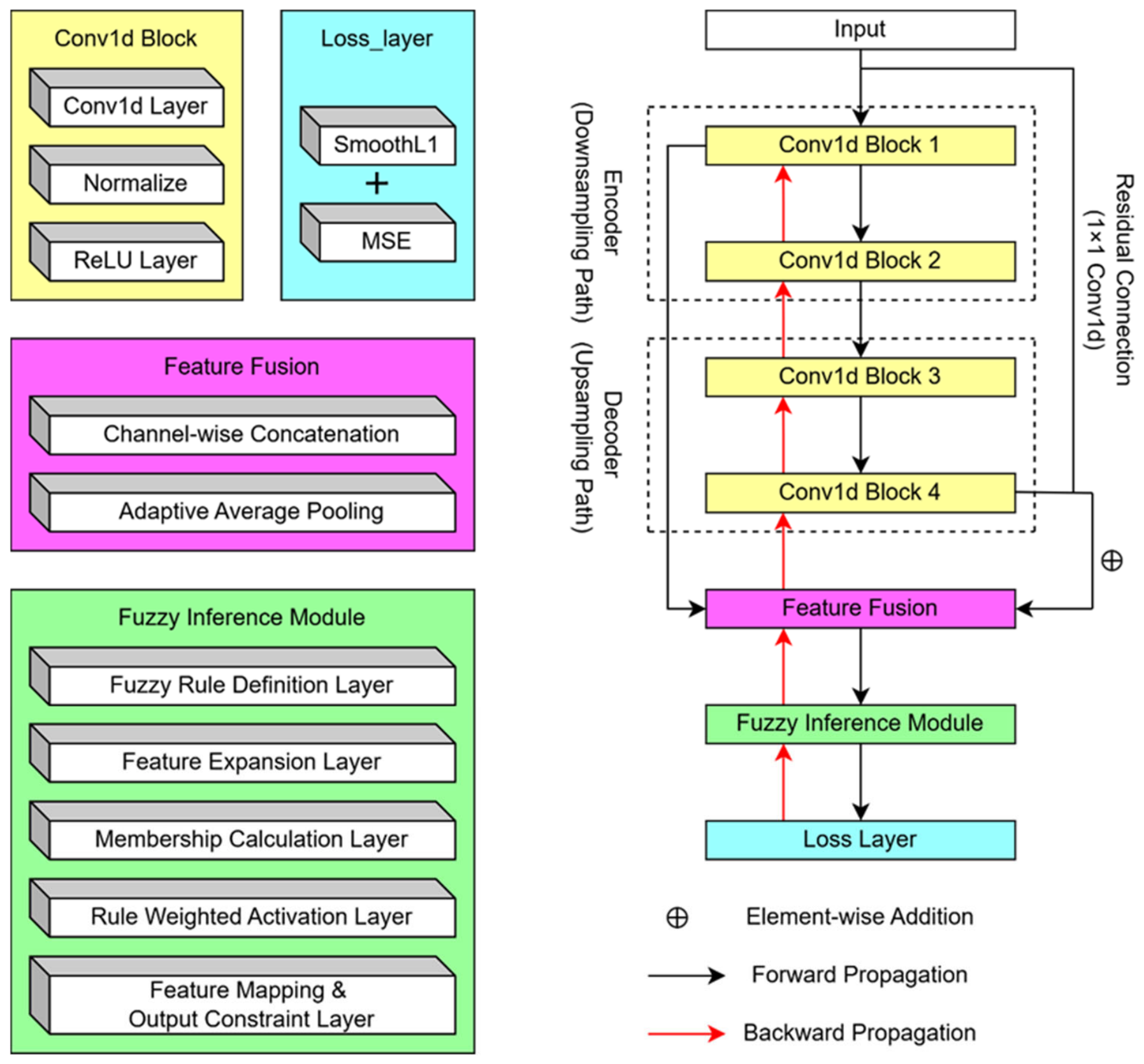
The proposed model mainly consists of two core components: a 1D U-Net module and a fuzzy inference module. The encoder–decoder architecture of the 1D U-Net enables the extraction and fusion of multi-scale features, which is well suited to the requirement of capturing local–global multi-scale damage features for the prediction of the residual ratio of ultimate bending moment. Meanwhile, the skip connection design of the 1D U-Net alleviates the gradient vanishing problem commonly encountered in deep network architectures, thereby improving the stability of model training, and exhibits favorable performance in feature learning from small datasets covering extreme damage conditions. For the fuzzy inference module, it converts damage input variables with inherent measurement errors into fuzzy sets with corresponding confidence levels via membership functions, which effectively mitigates the interference of measurement errors on prediction results and improves the robustness of the model. In addition, domain engineering prior knowledge can be incorporated into the model through the design of fuzzy rules, further enhancing the interpretability of the prediction outputs. The integration of the two modules addresses two key limitations of existing mainstream methods: insufficient capture of local–global multi-scale damage features, and the inherent black-box nature of pure data-driven models, thus improving the prediction accuracy and interpretability of the model simultaneously.

The 1D U-Net module is configured with 1 input channel, and both the base channel number and output channel number are set to 16. Each convolutional block is constructed by stacking a 1D convolution layer with a kernel size of 3 and padding of 1, followed by Batch Normalization (BN) and a Rectified Linear Unit (ReLU) activation function. Residual connections are introduced into the 1D U-Net module to reduce feature information loss, and multi-scale feature fusion is realized via feature concatenation operations. Unlike the general multi-scale designs widely adopted in computer vision (CV) and other fields, this multi-scale fusion mechanism is customized for the prediction of the residual ratio of the ultimate bending moment of damaged ship hull girders. Specifically, the shallow-layer detailed features extracted by the encoder are taken as local-scale features, while the final deep-layer features processed by residual connections are adopted as global-scale features. Cross-level feature fusion is completed through feature concatenation, which provides reliable input for the stable operation of the subsequent fuzzy inference module.

The fuzzy inference module is configured with five fuzzy inference rules to characterize the hull damage degree, and the rule design is aligned with five categories of ship damage conditions, i.e., negligible, minor, moderate, severe, and extreme damage [23]. Since more severe hull damage exerts a more significant impact on the residual ratio of ultimate bending moment and requires higher attention in structural safety assessment, the initial values of the rule weights are set to [0.1, 0.15, 0.2, 0.25, 0.3]. These weights are defined as trainable parameters, enabling adaptive adjustment of the rule weights under data-driven optimization. A triangular membership function is adopted to complete the fuzzification of each input feature, with membership centers set to [0.1, 0.3, 0.5, 0.7, 0.9] and a unilateral width of 0.1. This equidistant grading design is consistent with the engineering law of hull damage, which can realize full coverage of the normalized damage domain, while avoiding abrupt changes in rule activation or insufficient rule discrimination caused by inappropriate width settings. The rule activation degree is obtained by weighted summation of the membership values and rule weights, which is flattened and input into the fully connected (FC) layer. The FC layer adopts Xavier uniform initialization, with the initial bias value set to 0.01. The final output is soft constrained to the interval [0, 1] via Sigmoid activation, which matches the physical value range of the residual ratio of ultimate bending moment.

To obtain the theoretical basis of the model prediction, the activated fuzzy rules and corresponding rule weights can be directly extracted, thus realizing the interpretability of the prediction outputs. The overall framework of the proposed model is illustrated in Figure 1.

2.2. 1D U-Net Module

(1)

Convolutional Block

The basic operational unit of the network is the one-dimensional convolutional block, whose mathematical expression is given as:

$$f^l=\mathrm{ReLU}(\mathrm{BN}(\mathrm{Conv}1\mathrm{d}(f^{l-1}))),$$

(1)

where $f^l$ denotes the output feature of the l-th layer; Conv1d represents the one-dimensional convolution operation; BN is the batch normalization layer; ReLU is the nonlinear activation function.

(2)

Encoder–Decoder Architecture and Residual Connection

The network adopts an encoder–decoder architecture, where both the encoder and decoder contain two layers of convolutional blocks, which are designed to extract shallow-layer detailed features and deep-layer global features, respectively. Meanwhile, residual connections are introduced to achieve information enhancement and avoid the feature degradation problem during small-sample model training. The mathematical expression of the residual connection is given as:

$$x_{deep}=x_4+\mathrm{Conv}1{\mathrm{d}}_{1\times 1}(x),$$

(2)

where $x_{deep}$ denotes the final deep-layer features after residual connection; $x_4$ represents the deep-layer features output by the second convolutional block of the decoder; $x$ is the original input feature of the model; and $\mathrm{Conv}1{\mathrm{d}}_{1\times 1}( )$ is the 1 × 1 convolution for dimension matching.

(3)

Multi-scale Feature Fusion

The network realizes multi-scale feature fusion via feature concatenation operation so as to provide reliable feature input for the subsequent fuzzy inference module. Its mathematical expression is given as:

$$x_{fuse}=\mathrm{Concat}(x_1,x_{deep}),$$

(3)

where $\mathrm{Concat}( )$ denotes the feature concatenation operation; $x_{fuse}$ represents the multi-scale fused features obtained via the concatenation operation; $x_{deep}$ is the final deep-layer features after residual fusion; and $x_1$ is the shallow-layer detailed features extracted by the encoder.

2.3. Fuzzy Inference Module

(1)

Fuzzy Membership Calculation

The membership function is required to satisfy the following characteristics: (a) High computational efficiency and favorable gradient stability; (b) functional characteristics that are consistent with the engineering logic of hull damage degree classification and can achieve clear discrimination between adjacent damage grades; and (c) parameters of the function that have explicit and corresponding engineering implications. Among various common membership functions, the triangular membership function is a favorable candidate for this study. Its mathematical expression is given as:

$${\mu }_k(x)=\max (1-{\displaystyle \frac{\left|x-c_k\right|}{w_k}},0),$$

(4)

where ${\mu }_k(x)$ denotes the membership degree of the input feature to the k-th fuzzy rule; x represents the specific value of each feature element in $x_{fuse}$; $c_k$ is the center of the k-th fuzzy rule, corresponding to the standard representative value of each damage grade in the normalized interval; and $w_k$ is the width of the k-th fuzzy rule, corresponding to the coverage interval of each damage grade.

(2)

Weighted Activation of Fuzzy Rules and Output Mapping

The total activation degree of fuzzy rules is obtained by learnable weighted summation of the membership values. Subsequently, the activated features are flattened and mapped via the FC layer, and the final output is constrained to the physically valid interval [0, 1] using the Sigmoid activation function. Its mathematical expression is given as:

$${\alpha }_k={\theta }_k{\displaystyle {\sum }_{c=1}^C{\displaystyle {\sum }_{l=1}^{\mathrm{L}}{\mu }_k(x_{c,l})}},$$

(5)

$$\widehat{y}=\sigma (\mathit{W}\cdot \mathrm{Flatten}(\mathit{\alpha })+\mathit{b}),$$

(6)

where ${\alpha }_k$ denotes the activation degree of the k-th fuzzy rule; ${\theta }_k$ represents the learnable weight of the k-th fuzzy rule; C is the total number of channels; L is the total length of the feature; $x_{c,l}$ is the specific value of the element at the c-th channel and l-th length position in $x_{fuse}$; $\widehat{y}$ is the final output of the model; $\sigma ( )$ is the Sigmoid activation function; W and b is the weight matrix and bias vector of the FC layer; $\mathrm{Flatten}( )$ is the feature flattening operation function; and α is the vector composed of the activation degrees of all fuzzy rules.

2.4. Loss Function

In this study, a weighted hybrid loss function combining the SmoothL1 loss function and Mean Squared Error (MSE) loss function is designed. The SmoothL1 loss function, characterized by favorable robustness to outlier anomalies and stable gradient properties, is adopted to accommodate the core characteristics of the dataset—a wide span of sample damage conditions and the inclusion of extreme damage cases—so as to ensure the stability of model training. The MSE loss function, which features high fitting accuracy for continuous values and fast convergence speed, is introduced to match the characteristics of a high proportion of samples under conventional damage conditions and the continuous physical quantity attribute of the prediction target, thus balancing the anti-interference ability of model training and engineering prediction accuracy.

The mathematical expression of the SmoothL1 loss function is given as:

$${\mathrm{L}}_{\mathrm{SmoothL}1}=\left\{\begin{array}{l}0.5{(y-\widehat{y})}^2 , \left|y-\widehat{y}\right|<1\\ \left|y-\widehat{y}\right|-0.5 , \mathrm{otherwise}\end{array}\right.$$

(7)

The mathematical expression of the MSE loss function is given as:

$${\mathrm{L}}_{\mathrm{MSE}}={\displaystyle \frac{1}{N}}{\displaystyle {\sum }_{i=1}^N{(y_i-{\widehat{y}}_i)}^2}$$

(8)

where y denotes the ground truth value; $\widehat{y}$ represents the predicted value of the model; and N is the total number of samples.

The total loss function ${\mathrm{L}}_{total}$ is formulated by the weighted fusion of the two loss functions:

$${\mathrm{L}}_{total}=\alpha {\mathrm{L}}_{\mathrm{SmoothL}1}+(1-\alpha ){\mathrm{L}}_{\mathrm{MSE}}$$

(9)

To determine the optimal weight coefficient α, a univariate grid search method is adopted for hyperparameter optimization in this study. With all other experimental variables kept completely consistent, the influence of different α on the prediction performance of the model is compared, and the specific results are shown in

Table 1. Prediction errors under different α.

α	MAE	RMSE
0	0.024800	0.032179
0.1	0.022342	0.028568
0.2	0.029869	0.035047
0.3	0.024515	0.029150
0.4	0.025079	0.030174
0.5	0.024351	0.029086
0.6	0.025453	0.031081
0.7	0.024914	0.030412
0.8	0.021394	0.026276
0.9	0.027583	0.033839
1	0.029398	0.034855

.

It can be seen that the prediction error reaches the minimum when the α is set to 0.8. Therefore, the weight of the SmoothL1 loss function in the total loss function is determined as 0.8, and the weight of the MSE loss function is set to 0.2 accordingly.

2.5. Hyperparameters

All hyperparameters and random seeds are fixedly set to eliminate the interference of stochastic factors on the experimental results.

For the two key hyperparameters, namely, the batch size and initial learning rate, a univariate grid search method is adopted for hyperparameter optimization in this study. With all other experimental variables kept completely consistent, the effects of different batch sizes and initial learning rates on the prediction performance of the model are compared, and the specific results are shown in

Table 2. Prediction errors under different batch sizes.

Batch Sizes	MAE	RMSE
4	0.021641	0.027940
8	0.017924	0.023909
16	0.021394	0.026276
32	0.028233	0.033870

and

Table 3. Prediction errors under different initial learning rates.

Initial Learning Rates	MAE	RMSE
0.0001	0.026178	0.031525
0.0005	0.017924	0.023909
0.001	0.018445	0.026021
0.005	0.020624	0.026923

, respectively.

According to the experimental results, the optimal batch size and initial learning rate are determined as 8 and 0.0005, respectively.

Meanwhile, a learning rate scheduler is introduced during the model training process to optimize the convergence behavior of the model. When configuring the hyperparameters, this study does not aim to achieve the global absolute optimal hyperparameter configuration. Therefore, the univariate grid search for hyperparameter optimization is only performed on three core hyperparameters: the weight coefficient α of the weighted hybrid loss function, the optimal batch size, and the initial learning rate. The rest of the hyperparameters are set to the commonly used values in deep learning model training, and the specific values are listed in

Table 4. Core training hyperparameters.

Hyperparameter	Value
Batch Size	8
Initial Learning Rate	0.0005
Weight Decay	0
Optimizer	Adam
Gradient Clipping Maximum Norm	1.0
Global Random Seed	39

and

Table 5. Optimizer and learning rate scheduler hyperparameters.

Hyperparameter	Value
Optimization Mode	min
Decay Factor	0.5
Scheduler Patience	20
Minimum Learning Rate	5 × 10−6
Effective Decay Threshold	1 × 10−5

.

3. Dataset Description

3.1. Data Generation and Modeling Conditions

The dataset is derived from a law enforcement patrol vessel with the following principal dimensions: L_BP = 110 m, B = 16 m, D = 8 m, and T = 4 m. The structural scantlings at midship are: 12 mm thick main deck for the side shell and bottom plating; 8 mm thick for the inner bottom plating and longitudinal bulkheads; and longitudinal stiffeners consisting of 200 × 8 mm and 100 × 10 mm T-sections, plus HP 80 × 5 bulb flats.

Focusing on the side-hull damage in the form of side opening, which is commonly observed during ship operation, a dataset is established by calculating the residual ultimate bending moment of the hull under different damage conditions via the modified Smith method.

This method was first proposed by Fujikubo et al. [24]. It addresses the inherent limitation of the conventional Smith method, which fails to account for the neutral axis rotation effect and thus cannot accurately calculate the strength of asymmetrically damaged cross-sections, by deriving a set of explicit expressions to solve for both the translation and rotation of the neutral axis.

Subsequently, Li et al. [25] established a method for determining the neutral axis of asymmetric cross-sections integrated with the Multi-Objective Particle Swarm Optimization (MOPSO) algorithm and verified its effectiveness based on the Dow 1/3 frigate test model. Furthermore, Kuznecovs et al. [1] demonstrated that the results of the modified Smith method exhibited good agreement with those obtained from high-fidelity finite element simulations and proposed that a small number of finite element simulation results can be used to further calibrate the outputs of the modified Smith method.

The detailed calculation procedure of the modified Smith method is presented as follows:

(a)

Cross-section discretization. Following the framework of the conventional Smith method, the hull girder cross-section is discretized into two types of basic elements: hard corner elements and stiffened plate elements.

(b)

Determination of σ-ε constitutive models. The discretized elements are grouped according to their structural failure modes, and their corresponding σ-ε constitutive models are determined based on the IACS Common Structural Rules for Bulk Carriers and Oil Tankers (Harmonized) (CSR-H).

(c)

Determination of the cross-sectional neutral axis. Following the work of Li et al. [25], the MOPSO algorithm is adopted to locate the neutral axis of the cross-section. The convergence criteria of the algorithm are specified as the force balance error f₁ ≤ 0.01 and the force vector balance error f₂ ≤ 0.01.

(d)

Progressive curvature increment and ultimate strength calculation. The curvature is incrementally increased to obtain the moment–curvature relationship curve, from which the ultimate bending moment of the ship hull girder is derived.

Specifically, the dataset is constructed in accordance with the input and output parameters required for the modified Smith method calculation, with the construction conditions specified as follows.

(a)

Damage Location and Pattern

The entire hull is divided into Stations 0 to 19 from bow to stern, with corresponding damage conditions set for each station. Each damage condition contains only one single opening, whose longitudinal coverage along the ship length is entirely contained within the longitudinal interval of the ship length corresponding to a single calculation station. Therefore, the damage pattern is parametrically characterized by two core parameters: the opening height and the center position of the opening. The influence of other geometric irregularities is not considered in this study.

(b)

Opening Parameter Settings

The opening height ranges from 1000 mm to 2500 mm with an interval of 500 mm, and the center position of the opening is set from 0 mm to 1500 mm above the waterline with an interval of 500 mm, covering a total of 12 groups of damage size combinations. Owing to the limitation of sample size, the parameters are selected with a relatively large interval to ensure sufficiently distinguishable differences between different damage conditions so as to capture the variation law of structural responses induced by changes in damage conditions. The value ranges of the parameters are determined according to the molded depth of the target ship to ensure that the opening range does not exceed the molded depth of the hull.

(c)

Ultimate Bending Moment Calculation

The hogging and sagging ultimate bending moments of the hull are calculated based on the modified Smith method to obtain the residual ratio of ultimate bending moment of the hull under different opening parameter conditions.

3.2. Basic Data Composition

The cross combination of the aforementioned damage locations and opening parameters yields a total of 240 valid samples. The information contained in each sample and its corresponding physical role are detailed in

Table 6. List of sample information.

Calculation Station	Opening Height	Distance from Opening Center to Waterline	Section Modulus in Intact Condition	Still Water Bending Moment in Intact Condition	Residual Ratio of Hogging Ultimate Bending Moment	Residual Ratio of Sagging Ultimate Bending Moment
0	0	0	X	X	X	X
1	0	0	X	X
······
10	X	X	X	X
······
18	0	0	X	X
19	0	0	X	X

and

Table 7. Physical role of sample input features.

Features	Physical Role
Calculation Station	Characterizes the longitudinal position of the opening along the hull, reflects the differences in structural strength and mechanical properties of different hull sections, and provides the model with features of longitudinal structural variation.
Opening Height	Characterizes the size of the opening, and together with the distance from the opening center to the waterline, reflects the effective load-bearing area of the hull cross-section and residual bending capacity.
Distance from Opening Center to Waterline	Characterizes the vertical position of the opening within the hull cross-section, and together with the opening height, reflects the effective load-bearing area of the hull cross-section and residual bending capacity.
Section Modulus in Intact Condition	Provides a unified cross-section strength benchmark for different damage conditions and reflects the difference in structural strength at different longitudinal positions of the hull.
Still Water Bending Moment in Intact Condition	Reflects the initial load level at different longitudinal positions and provides initial conditions for bending moment redistribution after hull damage.
Residual Ratio of Hogging/Sagging Ultimate Bending Moment	Characterizes the attenuation ratio of the overall ultimate load-bearing capacity of the damaged hull relative to the intact condition and is adopted as the prediction target of the model to reflect the impact of damage on hull structural safety.

, respectively. For intact calculation stations, the opening-related parameters are set to 0, and X represents the specific numerical value in the tables.

In this study, the residual ratio of ultimate bending moment, rather than the absolute residual ultimate bending moment, is selected as the prediction target in order to eliminate the scale dependence of calculation results and improve the learning performance of the model.

3.3. Data Preprocessing

• Normalization

Min-max linear normalization is performed on input features to map all parameters to the [0, 1] interval, eliminating the impact of dimensional differences on model training.

• Dataset Splitting

The dataset is split into training, validation and test sets at a 7:1.5:1.5 ratio via stratified random sampling, being stratified by opening parameters. This strategy ensures consistent damage condition distribution across subsets and supports evaluation of the model’s interpolation prediction capability within the predefined parameter domain. Detailed splitting results are shown in

Table 8. Detailed dataset splitting results.

Dataset Split	Sample Count	Function
Training Set	168	Model parameter training and iterative optimization
Validation Set	36	Hyperparameter tuning, fitting monitoring, and early stopping triggering
Test Set	36	Model generalization performance and prediction accuracy evaluation

.

3.4. Dataset Characteristics and Limitation Statement

The dataset adopted in this study contains 240 groups of damage conditions. The residual ratio of ultimate bending moment for all conditions is calculated and solved via the modified Smith method, and each damage condition has a complete and consistent input–output parameter mapping relationship. This dataset is a structured dataset generated via parametric grid sampling, rather than a dataset collected from heterogeneous real-world ship accident cases.

The dataset adopted in this study is applicable to the development of a preliminary surrogate model within the predefined side damage parameter domain, and it is meant to replace the time-consuming modified Smith method calculations and realize rapid prediction of the residual ratio of ultimate bending moment. The transferability of the model trained on this dataset to other ship types and other damage patterns requires further validation.

4. Experimental Validation

4.1. Evaluation Metrics and Model Training Results

Commonly used evaluation metrics for neural network prediction models include the MAE, RMSE, and Coefficient of Determination (R²). The proposed fuzzy inference module in this study is designed to align the prediction results with the engineering physical laws of the hull’s residual ratio of ultimate bending moment and to perform rationality correction on the prediction outputs, rather than merely fitting the numerical distribution of the raw data. As a statistical goodness-of-fit metric, the R² is targeted at minimizing the sum of squared residuals, without considering the engineering rationality of the prediction results, which leads to a conflict with the optimization logic of the fuzzy inference module. Using the R² as the evaluation metric cannot reflect the optimization value of the fuzzy inference module in aligning with hull engineering physical laws, nor can it characterize the practical engineering prediction performance of the model. Therefore, only the MAE and RMSE are selected as the core evaluation metrics in this study: these two metrics are directly related to the error tolerance in engineering applications and can intuitively reflect the deviation between the model predicted values and the ground truth values.

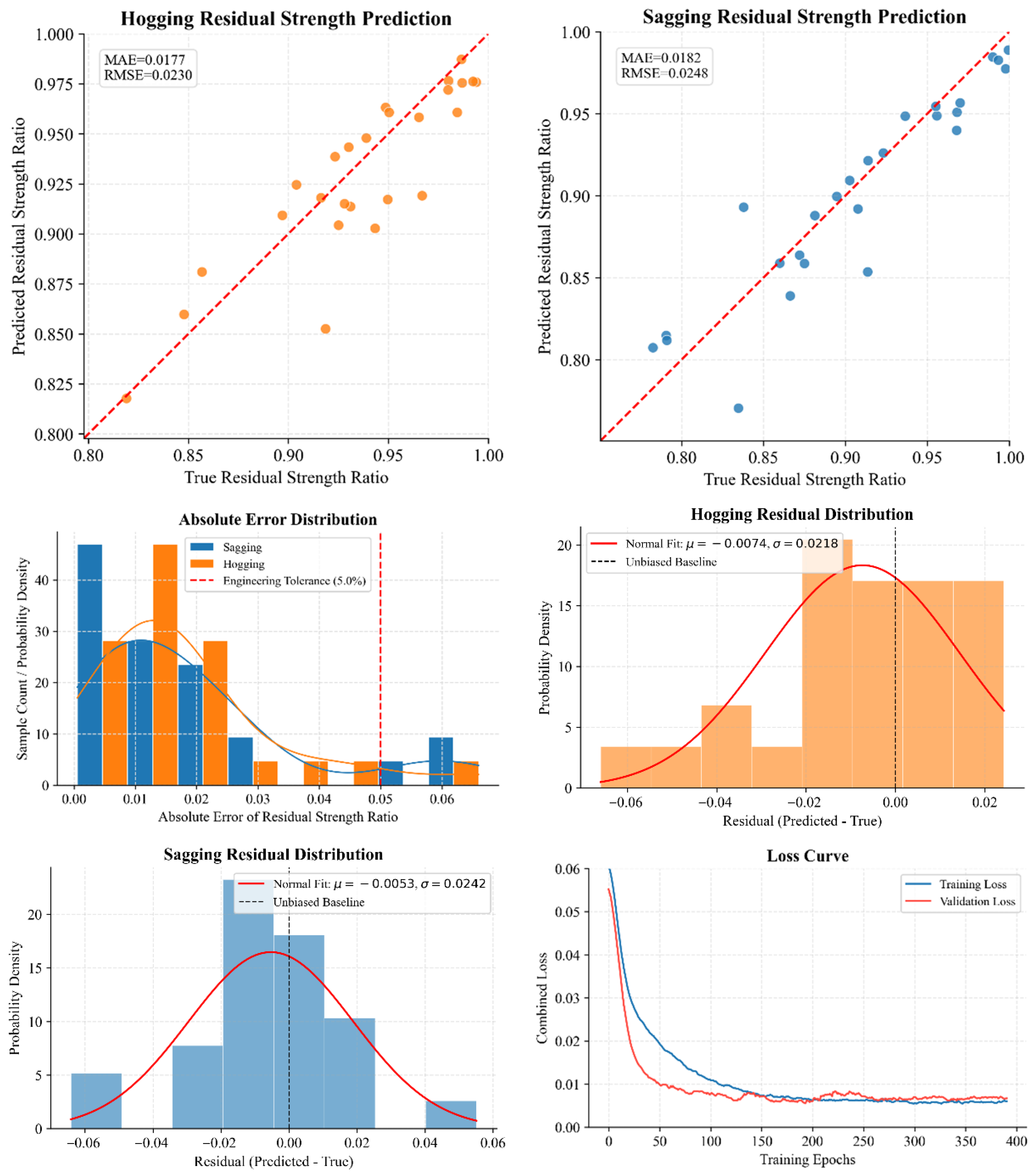
The model training and prediction results are shown in Figure 2.

It can be seen from Figure 2 that most sample data points of the model under both hogging and sagging conditions are in good agreement with the ideal fitting line, with the MAE below 2% and RMSE below 2.5% for both conditions. The absolute prediction errors of most samples are concentrated in the interval of 0~3%, and the error distribution presents a significant left-skewed characteristic, with no catastrophic large errors exceeding the safety threshold. The fitted means of the normal distribution of the residuals under hogging and sagging conditions are −0.0074 and −0.0053, respectively. There is no obvious left-skewed or right-skewed trend in the residual distribution, and no significant systematic deviation is observed in the prediction results. During the first 100 training epochs, the validation loss and training loss of the model decrease rapidly and synchronously. The loss curves tend to be stable after 150 epochs, and no overfitting phenomenon is observed.

4.2. Comparative Experiments

(1)

Benchmark Prediction Models

Three widely used prediction models are selected as benchmarks for comparison with the model proposed in this study, including the Support Vector Regression (SVR), Extreme Gradient Boosting Regression (XGBoost), and Multilayer Perceptron (MLP). In the comparative experiments, the consistency of the dataset, input and output settings, and training configuration are strictly controlled. Meanwhile, the total number of trainable parameters of all neural network models is controlled within the same order of magnitude to ensure the fairness of the comparative experiments.

(2)

Empirical Formula Calculation

For the calculation of the residual ultimate bending moment of the hull cross-section where a single opening is located, three groups of widely recognized empirical formulas are currently available as follows:

The first group is the empirical formula recommended by the International Association of Classification Societies (IACS), with the form:

$$M_{hog,damage}=M_{hog}[1-0.7{\displaystyle \frac{d}{B}}]$$

(10)

$$M_{sag,damage}=M_{sag}[1-0.65{\displaystyle \frac{d}{B}}]$$

(11)

The second group is the empirical formula recommended by the China Classification Society (CCS), with the form:

$$M_{hog,damage}=M_{hog}\cdot e^{-0.6{\displaystyle \frac{d}{H}}}$$

(12)

$$M_{sag,damage}=M_{sag}\cdot e^{-0.55{\displaystyle \frac{d}{H}}}$$

(13)

The third group is the empirical formula proposed by Prof. Chen Bozhen [26], with the form:

$$M_{hog,damage}=M_{hog}[1-0.8{({\displaystyle \frac{d}{H}})}^{1.8}]$$

(14)

$$M_{sag,damage}=M_{sag}[1-0.75{({\displaystyle \frac{d}{H}})}^{1.7}]$$

(15)

In the above formulas, $M_{hog,damage}$ and $M_{sag,damage}$ denote the residual ultimate hogging bending moment and residual ultimate sagging bending moment of the hull, respectively; $M_{hog}$ and $M_{sag}$ denote the ultimate hogging bending moment and ultimate sagging bending moment of the intact hull, respectively; d denotes the opening diameter; B denotes the maximum width of the cross-section; and H denotes the maximum height of the cross-section.

In contrast to the modified Smith method adopted as the basis of the proposed model in this study, all the aforementioned empirical formulae derive the ultimate bending moment under damaged conditions by applying a reduction factor to the ultimate bending moment of the intact hull girder.

The parameters B and H correspond to the Section Modulus in Intact Condition in the dataset, serving as proxies for the initial structural strength of the hull girder. As evidenced by their functional roles in the formulae, these empirical approaches simplistically assume that larger cross-sectional dimensions correlate with higher structural strength, exerting a positive effect on the residual bending moment. By contrast, the parameter d corresponds to the damage height in the dataset, which characterizes the severity of the damage opening and exerts a detrimental effect on the residual bending moment. Notably, other critical damage characteristics, such as the Distance from Opening Center to Waterline, are not incorporated into these empirical formulations.

(3)

FE Simulation

A damage condition from the test set is selected for finite element simulation verification, which is sufficiently extreme to examine the prediction performance of the proposed model. Specifically, the opening height is set to 2500 mm, which is consistent with the maximum opening height in the dataset; the opening is located at Station 10, with the opening center 500 mm above the waterline. The finite element simulation is performed in Abaqus (Dassault Systèmes, Vélizy-Villacoublay, France). The FE model is established based on the intact hull, a three-compartment hull segment with a total length of 20 m is extracted from the midship region, and the damage opening is simplified as a circular shape. The detailed specifications of the finite element model are presented as follows:

(a)

Element type. Three-dimensional reduced-integration quadrilateral shell elements (S4R) are adopted as the primary elements, supplemented by a small number of triangular shell elements (S3R) in regions with complex local geometries.

(b)

Mesh generation and convergence analysis. Using the 18 mm mesh as the reference benchmark, three mesh schemes with element sizes of 50 mm, 35 mm, and 25 mm are systematically compared. The 25 mm mesh is finally selected, as its simulation results exhibit an error of approximately 1.2% compared with those of the 18 mm reference mesh, while the total number of elements (approximately 450,000) is only 60% of that of the 18 mm mesh. This configuration strikes an optimal balance between computational accuracy and cost, which aligns with practical engineering requirements.

(c)

Material properties. The material is marine mild steel governed by the isotropic hardening von Mises yield criterion, with a Poisson’s ratio ν = 0.3, Young’s modulus E = 2.06 × 10⁵ MPa, and density ρ = 7.85 × 10⁻⁹ t/mm³. The material behavior is described by a true stress–strain curve defined by eight data points, as shown in

Table 9. Stress–strain data points for marine mild steel.

Yield Stress (MPa)	Plastic Strain
235.0	0
248.0	0.00124
294.5	0.03936
332.5	0.07749
362.0	0.11562
383.0	0.15370
395.7	0.19187
399.9	0.23000

, which covers the entire process from initial yielding to ultimate tensile failure.

(d)

Geometric imperfection treatment. The eigenvalue buckling mode method is employed to introduce initial geometric imperfections. The first-order buckling mode is extracted as the shape of the initial geometric imperfection, with an imperfection amplitude set to 5% of the plate thickness.

(e)

Boundary conditions and loading. Two reference points, RP-1 and RP-2, are created at the centroids of the forward and aft end faces of the model, respectively. Kinematic coupling constraints are applied to rigidly connect all nodes on each end face to their corresponding reference point. RP-1 is defined as the loading end, where the translational degrees of freedom in non-loading directions are constrained, and a prescribed rotation is applied. RP-2 is defined as the simply supported end, where all translational degrees of freedom are constrained.

(f)

Structural collapse criterion. The peak point of the moment–curvature curve is defined as the ultimate bending moment. Structural collapse is deemed to occur when the bending moment drops below 90% of the peak value or when convergence failure of the Riks arc-length solver is encountered, which indicates a complete loss of load-carrying capacity of the structure.

The total time from the start of modeling to the acquisition of the calculation result is about 15 min.

4.3. Results Analysis

4.3.1. Effect Analysis of Data Augmentation

It is widely recognized in deep learning that data augmentation is commonly required during model training with small sample datasets to mitigate issues such as model overfitting. To verify the practical effect of data augmentation under the research conditions of this study, Gaussian noise injection, a widely adopted optimization strategy in small-sample learning, is selected for data augmentation implementation. The intensity of Gaussian noise is constrained to a reasonable range, as excessive noise intensity may generate synthetic data inconsistent with engineering practice. In this study, Gaussian noise with a mean of 0 and a standard deviation of 0.005 is adopted to perturb the normalized input features. The prediction errors before and after data augmentation are listed in

Table 10. Comparison of prediction errors before and after data augmentation.

Error Metric	Without Data Augmentation	With Data Augmentation
Overall MAE	0.017924	0.025496
Sagging MAE	0.018157	0.025989
Hogging MAE	0.017691	0.025004
Overall RMSE	0.023909	0.032023
Sagging RMSE	0.024802	0.031567
Hogging RMSE	0.022981	0.032472

.

It can be seen from Table 10 that, compared with the benchmark model without data augmentation, the prediction accuracy of the model with the above augmentation process is decreased. This phenomenon is mainly attributed to three aspects:

(a)

The Gaussian noise introduced by data augmentation disrupts the inherent physical meaning of the input features, which may lead the model to learn spurious mapping relationships.

(b)

The fuzzy inference module relies on well-defined feature values for membership calculation and fuzzy rule activation, and noise interference will cause disorder in the activation degree of fuzzy rules.

(c)

The original input features already cover the core engineering indicators required for the prediction of the residual ratio of ultimate bending moment. The additional noise-based augmentation does not increase the effective diversity of the dataset but increases the learning burden of the model.

This result verifies that for the model proposed in this study, untargeted random noise augmentation should be avoided, and data augmentation should be implemented with samples consistent with the actual engineering logic of hull damage.

4.3.2. Interpretability Analysis

To verify the interpretability of the proposed fuzzy inference module, a sample from the test set is selected for case analysis in this section. For this sample, the opening is located at Station 10, with an opening height of 2500 mm and the opening center 500 mm above the waterline. The residual ratios of ultimate bending moment under sagging and hogging damage conditions are 86.6% and 92.8%, respectively.

The activated fuzzy rules and corresponding weights under this damage condition are shown in

Table 11. Fuzzy rules and corresponding weights.

Fuzzy Rule	Initial Weight	Post-Training Weight	Rule Activation Degree Under This Damage Condition
Negligible Damage	0.1	0.4102	5.9104
Minor Damage	0.15	0.3775	2.6656
Moderate Damage	0.2	0.4218	4.0428
Severe Damage	0.25	0.5134	4.3100
Extreme Damage	0.3	0.4758	7.3922

.

It can be seen from Table 11 that the weights of all rules are adaptively updated after training with the dataset, indicating that the fuzzy inference module effectively participates in the model learning process. Under this damage condition with the maximum opening diameter, each rule presents a distinct activation level. Among them, the Extreme Damage rule has the highest activation degree, which indicates that the model can accurately identify the extreme damage state and is consistent with the predefined physical laws.

Meanwhile, the Negligible Damage rule also presents a relatively high activation degree. This is mainly attributed to the fact that the input features include the section modulus in intact condition, which is a core mechanical characteristic of the hull. The high section modulus at the mid-ship region enables the model to take the strong initial load-bearing capacity of the structure into account during inference, thus leading to a notable response of this rule. From the perspective of the residual ratio of ultimate bending moment, even with a large opening, the residual ratio of ultimate bending moment remains at a relatively high level, which verifies that the activation of the Negligible Damage rule is sufficiently supported by the physical characteristics of the hull.

All rules present a certain level of activation, and no extreme case with negligible activation degree is observed. This demonstrates that the fuzzy rules designed in this study are reasonable, with no redundant or invalid rules. Meanwhile, it also verifies that the model has a relatively balanced perception capability for damage features of different degrees, and no feature bias problem is detected. The above results further confirm that the fuzzy inference module operates stably and effectively participates in the model decision-making process.

4.3.3. Analysis of Engineering Application Advantages

To verify the engineering application performance of the model proposed in this study, a horizontal comparison is conducted between the prediction results of the proposed model and those of other benchmark prediction models, empirical formula calculations, and FE simulations. The performance comparison of different prediction models is shown in

Table 12. Performance comparison of different prediction models.

Error Metric	The Proposed Model	SVR	XGBoost	MLP
Overall MAE	0.017924	0.054241	0.028372	0.039024
Sagging MAE	0.018157	0.052063	0.029296	0.045775
Hogging MAE	0.017691	0.056418	0.027447	0.032273
Overall RMSE	0.023909	0.062156	0.037759	0.045479
Sagging RMSE	0.024802	0.062127	0.038294	0.052388
Hogging RMSE	0.022981	0.062185	0.037218	0.037311

.

It can be seen from Table 12 that the XGBoost model achieves the highest prediction accuracy among the selected benchmark prediction models, with an overall MAE of 2.83% and an overall RMSE of 3.78%. By comparison, the proposed model yields an overall MAE of 1.79%, which is 1.04 percentage points lower than that of the XGBoost model, and an overall RMSE of 2.39%, which is 1.39 percentage points lower than that of the XGBoost model. This result indicates that the proposed model has better adaptability to the task of rapid prediction of the residual ratio of ultimate bending moment and verifies the rationality and necessity of the proposed model design.

The comparison between the model prediction results and the calculation results of three groups of empirical formulas for rapid estimation of residual bending moment of hulls with a single opening is shown in

Table 13. Error comparison between model prediction and empirical formula calculation.

Error Metric	The Proposed Model	The First Group of Empirical Formulas	The Second Group of Empirical Formulas	The Third Group of Empirical Formulas
Overall MAE	0.017924	0.076288	0.122567	0.095656
Sagging MAE	0.018157	0.066792	0.107305	0.089202
Hogging MAE	0.017691	0.085784	0.137829	0.102110
Overall RMSE	0.023909	0.088917	0.136649	0.118361
Sagging RMSE	0.024802	0.083408	0.123419	0.114216
Hogging RMSE	0.022981	0.094104	0.148706	0.122366

.

It can be seen from Table 13 that the empirical formula recommended by IACS achieves the highest prediction accuracy among the three empirical formulas, with an overall MAE of 7.63% and an overall RMSE of 8.89%. In contrast, the proposed model yields an overall MAE of 1.79%, which is 5.84 percentage points lower than that of the most accurate empirical formula, and an overall RMSE of 2.39%, which is 6.50 percentage points lower than that of the most accurate empirical formula. This result indicates that the proposed model has higher prediction accuracy than classical engineering empirical formulas. It overcomes the limitation of single-factor simplification in traditional empirical formulas and can more accurately fit the variation law of residual bending moment of damaged hulls.

From the perspective of individual damage conditions, the two types of methods present distinct opposite trends in prediction accuracy: the empirical formulas achieve better prediction performance under sagging damage conditions, while the proposed model achieves higher prediction accuracy under hogging damage conditions. This difference is attributed to the combined effect of the characteristics of the dataset and the inherent properties of the prediction methods.

In engineering practice, structural buckling induced by compressive loads is the dominant failure mode leading to the degradation of structural load-bearing capacity, which has received more attention than tensile failure. For all damage conditions in the dataset, the opening center is generally closer to the deck, which means that the opening is located near the compression side under sagging conditions. Under this circumstance, the bending moment is mainly affected by the single factor of cross-sectional area loss, which exactly matches the calculation logic of empirical formulas that perform strength reduction based on opening size. Therefore, the empirical formulas yield higher prediction accuracy under sagging conditions than under hogging conditions. Under hogging damage conditions, the bending moment is affected by the coupling effects of multiple factors, including opening diameter, distance from the opening to the neutral axis, longitudinal position along the ship length, and cross-sectional stress gradient. The corresponding mechanical behavior is complex with strong nonlinear characteristics, which cannot be effectively captured by traditional empirical formulas.

For the proposed model, the optimization objective of minimizing global loss during training enables the model to allocate more fitting capacity to the sample regions with larger error contribution, more complex mechanical mechanisms, and more significant nonlinear characteristics, while allocating less learning resources to samples with clear variation laws, inherently low errors, and near-linear responses. Thus, the proposed model exhibits better prediction accuracy under hogging damage conditions. Specifically, the proposed model realizes automatic extraction of deep multi-dimensional features, including opening size, opening position, and cross-sectional characteristics via the U-Net architecture, which can effectively fit the multi-factor coupling effects under hogging conditions. Meanwhile, the fuzzy inference module constrains the prediction results based on engineering criteria, which further improves the engineering rationality of the prediction values under hogging conditions.

The comparison of the residual ratio of ultimate bending moment for the preselected damage condition between the model prediction and FE simulation is shown in

Table 14. Error comparison between model prediction and finite element simulation.

Method	Residual Ratio of Sagging Ultimate Bending Moment	Residual Ratio of Hogging Ultimate Bending Moment
The proposed model prediction	84.6%	90.3%
FE Simulation	82.1%	88.7%

.

Taking the FE simulation results as the reference values, the absolute error of the model prediction is 2.5 percentage points for the residual ratio of sagging ultimate bending moment and 1.6 percentage points for that under hogging condition. The prediction accuracy meets the engineering accuracy requirements, while the proposed model has significantly higher prediction efficiency than the 15-minute calculation duration of FE simulation, which is more consistent with the practical engineering requirements of maritime emergency assessment for damaged ships.

5. Conclusions

This study explores a technical framework for predicting the residual ultimate bending moment of damaged ships, which combines the nonlinear multi-feature fitting capability of deep learning with engineering prior knowledge of hull structural strength. The U-Net model integrated with a fuzzy inference module is adopted to predict the residual ratio of ultimate bending moment for ships with a single side opening, and the prediction results are compared with those obtained from other benchmark prediction models, empirical formula calculations, and finite element simulations. The results verify that the proposed model has favorable engineering application performance: it can realize rapid prediction of the residual ultimate bending moment while ensuring prediction accuracy and can meet the timeliness and reliability requirements in maritime emergency response scenarios.

Combined with the research scope of this study and practical engineering requirements, future research can be focused on the following two aspects: first, increasing the number of dataset samples and expanding the validation scope to further improve the generalization performance of the model; second, employing high-fidelity FE simulation data instead of the modified Smith method as the generation source for damage scenarios to construct a multi-task dataset annotated with multiple labels, including residual strength and flooding response. This will facilitate the training of a more holistic damage prediction model and extend the applicability of the proposed framework to a wider range of engineering scenarios. Meanwhile, future work can explore the integration of the proposed model with the ship emergency assessment system or adopt more advanced deep learning architectures, such as Transformer-based temporal networks combined with fuzzy inference for prediction, to further enhance the engineering application value of the method.