Article

Energy-Efficient Pitch Control for a 1000 m-Class Underwater Glider: A Comparative Study of PID, Fuzzy, and ANFIS Controllers Based on Experimental Power Models


1
Sea Power Reinforcement · Security Research Department, Korea Institute of Ocean Science and Technology, Busan 49111, Republic of Korea
2
Department of Ocean Advanced Materials Convergence Engineering, Korea Maritime & Ocean University, Busan 49112, Republic of Korea
*
Author to whom correspondence should be addressed.
J. Mar. Sci. Eng. 2026, 14(11), 986; https://doi.org/10.3390/jmse14110986 (registering DOI)
Submission received: 30 April 2026 / Revised: 18 May 2026 / Accepted: 20 May 2026 / Published: 26 May 2026
(This article belongs to the Special Issue Advances in Marine Autonomous Vehicles)

Abstract

Underwater gliders are suited for long-duration oceanographic observation, but their endurance is bounded by onboard energy capacity. An overlooked source of energy loss is the attitude control system, which repeatedly repositions the internal moving mass to hold the desired pitch angle throughout each gliding cycle. Conventional PID and manually tuned fuzzy controllers continue driving the actuator after pitch convergence and adapt poorly to nonlinear buoyancy variations at depth. To address this, we propose an ANFIS (Adaptive Neuro-Fuzzy Inference System)-based pitch control strategy for a 1000 m-class underwater glider. A nonlinear 6-DOF dynamic simulator incorporating experimentally derived power models for the buoyancy engine and attitude controller was validated up to 100 bar. A 13-rule Sugeno-type fuzzy inference system was optimized through ANFIS hybrid learning using approximately 5500 samples from PID steady-state data. Simulation results show energy savings of 57.05% over PID and 4.98% over a manually tuned fuzzy controller, with no degradation in tracking accuracy. Sea trials confirm a reduction in moving mass displacement under real disturbance conditions, providing qualitative evidence consistent with the simulation results. Further quantitative validation of the energy reduction effect through free-running sea trials remains as future work.

1. Introduction

1.1. Research Background

Underwater gliders are autonomous platforms that generate propulsive force through buoyancy changes and internal mass shifting. Since Stommel [1] first envisioned the concept, they have become indispensable tools for mid- and deep-ocean environmental monitoring, offering months-long endurance, broad spatial coverage, and fully independent operation [2].
Operational endurance is ultimately limited by onboard battery capacity, shared among the buoyancy engine, attitude controller, and heading controller. This constraint is especially pronounced in environments like the East Sea of Korea, where strong surface currents and sharp vertical density gradients [3,4] make it difficult to simultaneously sustain adequate forward speed, stable pitch regulation, and efficient energy use.
Pitch control strategies for underwater gliders span a broad spectrum. PID controllers remain the most widely used solution owing to their simplicity and reliability [5], while reinforcement learning combined with active disturbance rejection has also been explored [6]. To better handle the nonlinear dynamics and varying conditions inherent to glider operation, intelligent control methods have gained increasing attention, including fuzzy logic control [7], sliding mode control [8], and Sugeno-type fault-tolerant control [9]. Parallel efforts have examined attitude regulation mechanism design [10] and buoyancy engine performance characterization [11,12].
In Korea, a 1000 m-class underwater glider has been developed primarily through the Korea Institute of Ocean Science and Technology (KIOST) [3]. The authors were directly involved in its design and control system development, and the operational demands of the East Sea served as the primary motivation for this study.

1.2. Research Motivation and Problem Statement

Most energy optimization studies for underwater gliders have focused on buoyancy engine efficiency and motion pattern design [13,14,15], while energy losses from unnecessary attitude controller actuation have received little attention. The attitude controller regulates pitch angle by displacing the battery pack along the longitudinal axis, but under conventional PID control, error-driven corrections persist even after the pitch angle has converged, generating avoidable energy losses. These losses may appear negligible on a per-cycle basis, yet accumulate significantly over multi-month missions. Pycnocline passage further compounds the problem by inducing large pitch disturbances that demand sustained corrective action [16].
The nonlinear relationships among pitch angle error, desired pitch angle, and buoyancy control input make analytical optimization inherently difficult. Sugeno-type fuzzy controllers offer a practical framework for encoding these relationships as expert-defined inference rules [17], but manually tuned membership functions depend heavily on designer intuition and cannot reliably deliver energy-optimal performance. ANFIS [18] overcomes this by marrying the interpretability of fuzzy logic with the learning capacity of neural networks, enabling systematic, data-driven refinement of membership function parameters [19,20]. While ANFIS has been widely applied to AUV and underwater vehicle control, its application specifically targeting attitude controller energy minimization in underwater gliders remains limited. This study explores this direction by combining ANFIS with experimentally derived power models.
A further gap in existing work is the common practice of simplifying or assuming actuator power consumption rather than measuring it [13], which limits the credibility of simulation-based energy estimates. The present study addresses both gaps by integrating experimentally validated, pressure-aware power models into the simulation framework [12].

1.3. Research Objectives and Contributions

To address the challenges outlined above, this study proposes an ANFIS-based pitch control strategy built around experimentally derived actuator power models. The main contributions are as follows.
First, a high-fidelity glider simulator was developed by coupling a nonlinear 6-DOF dynamic model [21] with experimentally grounded actuator power models. Pressurization tests at up to 100 bar were used to characterize buoyancy engine pump speed and current draw as functions of PWM input and back-pressure, and a pitch-angle-dependent power model for the attitude controller was derived through polynomial regression and integrated into the simulator [12].
Second, a 13-rule Sugeno-type FIS [22] was designed from physical insight, using pitch angle error, desired pitch angle, and buoyancy control volume as inputs. A neutral output condition ( f 5 ) was explicitly built into the ZERO mode to suppress the hunting behavior that arises from moving-mass inertia after pitch convergence.
Third, ANFIS hybrid learning [18] was applied to refine the membership function parameters of the designed FIS. Approximately 5500 training samples were extracted from PID steady-state convergence responses, spanning buoyancy control volumes of 200–500 cc and desired pitch angles of −40° to +40°.
Fourth, the controller was validated through comparative simulations and sea trials conducted in the East Sea off Samcheok, Republic of Korea. Simulations confirmed a 57.05% energy reduction over PID, and sea trials demonstrated a marked reduction in moving mass displacement under real disturbance conditions.
The remainder of this paper is organized as follows. Section 2 describes the glider dynamic model and actuator power models. Section 3 details the design of the PID, Sugeno fuzzy, and ANFIS-based fuzzy controllers. Section 4 and Section 5 present the simulation and sea trial results, respectively, and Section 6 draws conclusions and outlines directions for future research.

2. Physical Modeling of the 1000 m-Class Underwater Glider

To accurately capture the glider’s motion, a nonlinear 6-DOF dynamic model is formulated based on the Newton–Euler equations. The model accounts for depth-dependent buoyancy variation under hydrostatic pressure and parameter changes driven by internal mass displacement.

2.1. Specifications of the Underwater Glider

The key specifications of the developed glider are listed in Table 1, and its external configuration is shown in Figure 1.

2.2. Coordinate System Definition and Motion Variables

2.2.1. Six-Degree-of-Freedom (6-DOF) Dynamic Modeling

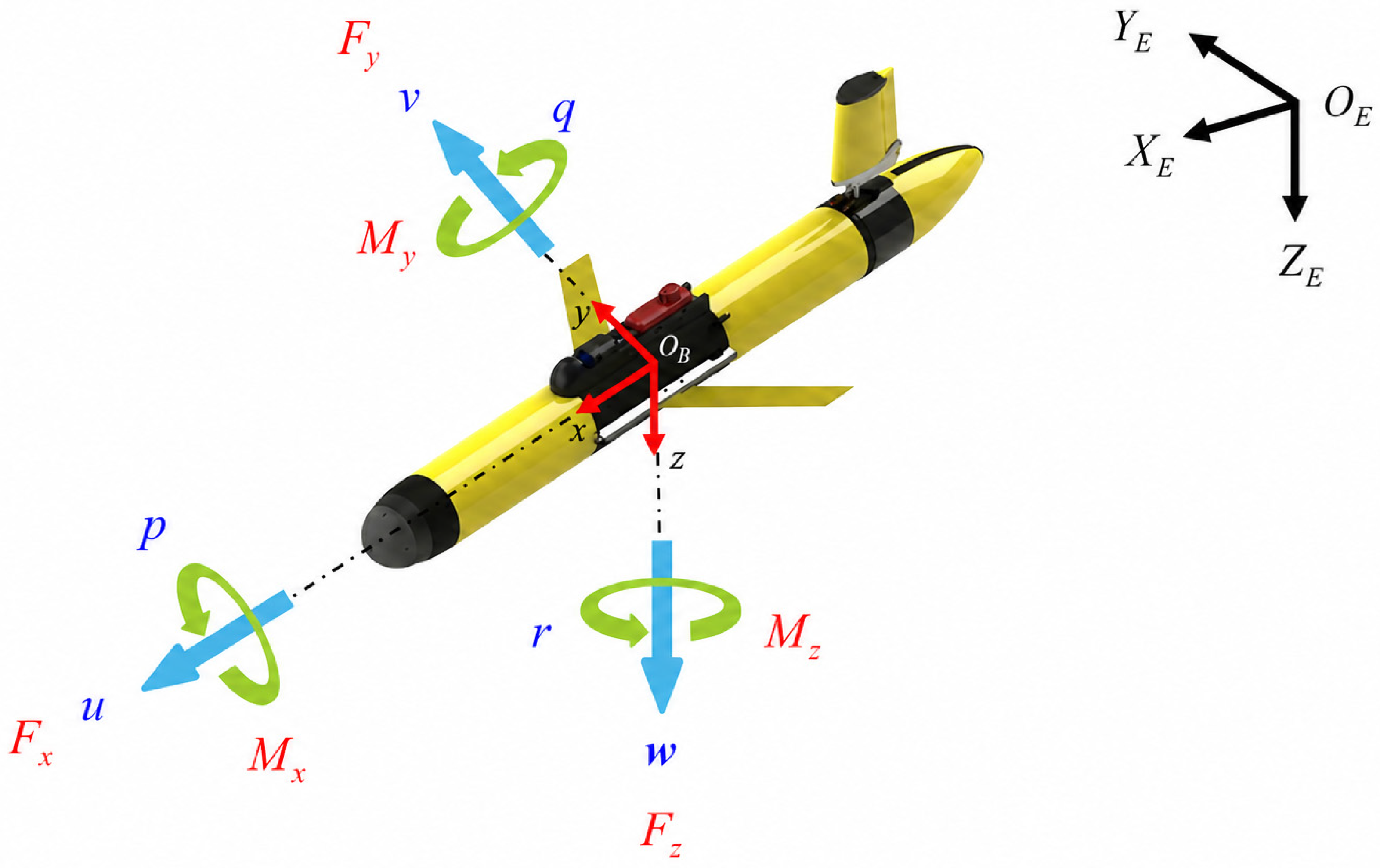
To describe the nonlinear motion characteristics of the underwater glider, an Earth-Fixed Frame O E and a Body-Fixed Frame O B are defined as illustrated in Figure 2.
The Earth-Fixed Frame O E is an inertial reference frame established at the sea surface, defining the absolute position and attitude of the underwater glider. The Body-Fixed Frame O B is a non-inertial frame fixed to the glider hull. The origin O B is located at the center of buoyancy, with the x-axis directed toward the bow (Forward), the z-axis directed downward (Downward), and the y-axis directed toward the starboard side (Starboard) in accordance with the right-hand rule.
The position and attitude vector η in the Earth-Fixed Frame and the linear and angular velocity vector ν in the Body-Fixed Frame are defined as follows:
η = [ x   y   z   ϕ   θ   ψ ] Τ ,     ν = [ u   v   w   p   q   r ] Τ
The kinematic relationship between the two coordinate frames is expressed as η ˙ = J ( η ) ν using the transformation matrix J ( η ) [21], where u ,   v and w denote the surge, sway, and heave velocities, respectively, and p ,   q and r denote the roll, pitch, and yaw angular velocities, respectively. The state variables corresponding to each degree of freedom are defined in Table 2.
The nonlinear 6-DOF equations of motion for the underwater glider are formulated incorporating the total mass m , the moment of inertia I , and the time-varying center of gravity r c g , which changes in real time according to control inputs. The gravitational force W and buoyancy B are derived from the buoyancy and mass motion model described in Section 2.2.2, and are computed in real time during simulation to serve as inputs to the equations of motion. The equations of motion for each degree of freedom are given as follows:
Surge :   m t o t a l u ˙ v r + w q x G ( q 2 + r 2 ) + y G ( p q r ˙ ) + z G ( p r + q ˙ ) = F x       Sway :     m t o t a l v ˙ w p + u r y G ( r 2 + p 2 ) + z G ( q r p ˙ ) + x G ( p q + r ˙ ) = F y       Heave :   m t o t a l w ˙ u q + v p z G ( p 2 + q 2 ) + x G ( p r q ˙ ) + y G ( q r + p ˙ ) = F z       Roll :   I x x p ˙ + I z z I y y q r I y z q 2 r 2 + I x y p r q ˙ I z x p q + r ˙ + m t o t a l y G ( w ˙ u q + v p ) z G ( v ˙ w p + u r ) = M x           Pitch :   I y y q ˙ + ( I x x I z z ) p r I z x ( r 2 p 2 ) + I y z ( p q r ˙ ) I x y ( q r + p ˙ )       + m t o t a l z G ( u ˙ v r + w q ) x G ( w ˙ u q + v p ) = M y       Yaw :   I z z r ˙ + ( I y y I x x ) p q I x y ( p 2 q 2 ) + I z x ( q r p ˙ ) I y z ( p r + q ˙ )         + m t o t a l x G ( v ˙ w p + u r ) y G ( u ˙ v r + w q ) = M z
The right-hand side terms F x ,   F y ,   F z ,   M x ,   M y   and M z collectively represent the hydrodynamic forces and moments acting on the glider, encompassing drag, lift, buoyancy, and gravity. The hydrodynamic derivatives used in the simulation were drawn from the established literature of Fossen [21], Graver [23], and Huang et al. [24], and non-dimensionalized before being incorporated into the 6-DOF dynamic model.

2.2.2. Buoyancy and Mass Motion Model of the Underwater Glider

Glider motion is governed by the interplay between net buoyancy changes and center-of-gravity shifts induced by internal mass displacement. The following subsections define the mathematical models for both the center of buoyancy (CB) and the center of gravity (CG).
Buoyancy Model and Center of Buoyancy (CB) Variation
The total buoyancy B of the underwater glider is defined as the sum of the static buoyancy generated by the fixed hull volume and the variable buoyancy induced by bladder volume changes. The variable buoyancy B represents the net buoyancy change, calculated as the weight of seawater displaced during bladder inflation ( V ρ w a t e r g ) minus the weight of hydraulic oil transferred into the bladder ( V ρ o i l g ). The volume change V and total buoyancy B as functions of the external piston radius r and displacement h are given by Equations (3) and (4):
B =   V × ( ρ w a t e r ρ o i l ) × g
B = [ V f i x × ρ w a t e r + V × ρ w a t e r ρ o i l ] × g
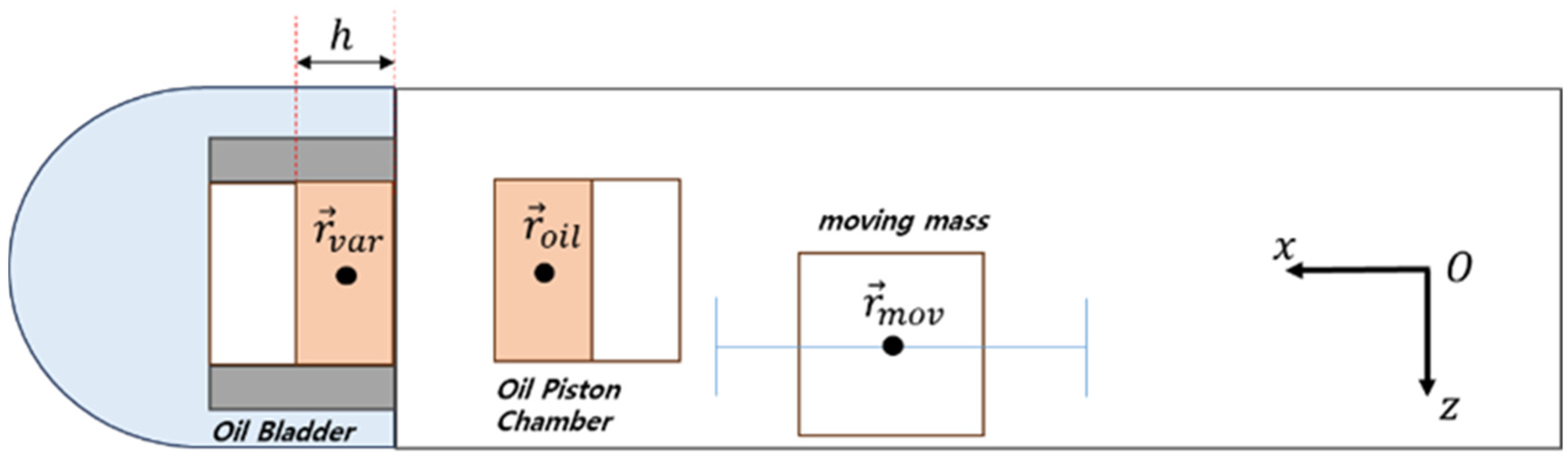
Figure 3 illustrates the arrangement of internal components of the underwater glider and the position vectors of each mass element, providing the geometric reference for computing the center of buoyancy and center of gravity.
The center of buoyancy r c b is computed as the weighted average of the fixed and variable buoyancy components, and is expressed as Equation (5):
r c b = x B y B z B =   B f i x r f i x + B v a r r v a r B f i x + B v a r
Mass Model and Center of Gravity (CG) Displacement
In this study, the interior of the hull is defined as the system boundary. Accordingly, the total mass of the underwater glider m t o t a l is calculated as the sum of all constituent elements existing within the hull. When the buoyancy engine is activated, hydraulic oil m o i l is discharged from the internal tank to the external bladder, reducing the total mass within the system boundary by the amount of expelled oil. Therefore, m t o t a l is treated as a dynamic variable incorporating variable mass components, and is defined as Equation (6):
W t o t a l = m t o t a l × g = ( m s t a t + m m o v + m o i l ) × g
where m s t a t denotes the fixed mass, m m o v the moving mass, and m o i l the residual hydraulic oil mass remaining within the hull. The reduction in total mass due to external oil discharge and the positional changes in internal components shift the system-wide center of gravity r c g , which is expressed by the principle of moment summation as Equation (7):
r c g = x G y G z G = m s t a t r s t a t + m m o v r m o v + m o i l r o i l m t o t a l  

2.3. Experimentally Derived Actuator Power Modeling

To assess the glider’s long-term operational capability, the power consumption characteristics of each actuator were experimentally quantified and incorporated into the simulation as numerical models. Since this study focuses on energy efficiency during vertical dive-and-rise cycles, the heading controller was excluded from the power modeling.

2.3.1. Buoyancy Engine Characterization and Experimental Configuration

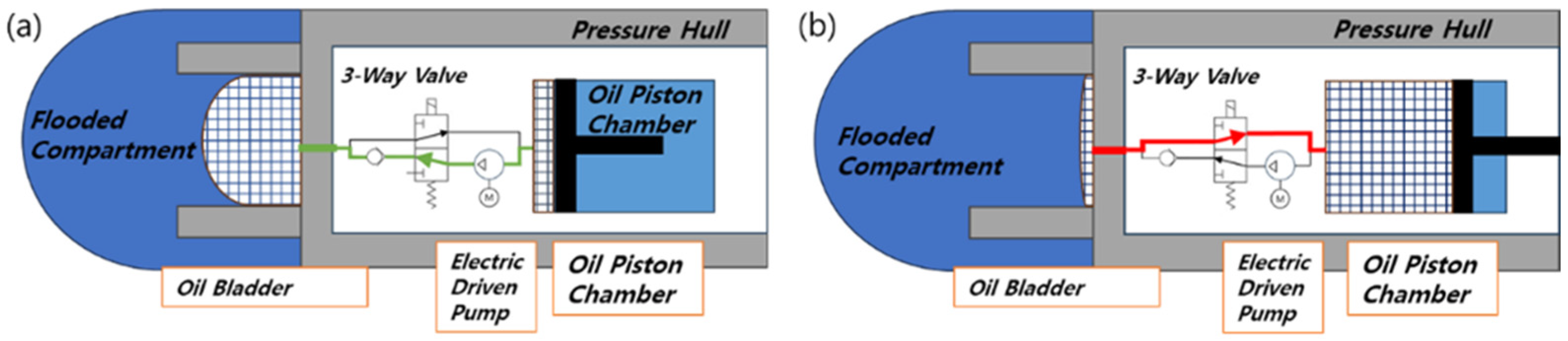
The buoyancy engine serves as the sole means of propulsion, driving the glider by alternately adjusting net buoyancy and effective hull mass. Figure 4 shows the hydraulic system configuration and operating principle. During ascent, the hydraulic pump actively forces oil into the external bladder to generate positive buoyancy, consuming electrical power in the process. During descent, oil is passively recovered by exploiting the pressure differential between the external water column and the internal tank, eliminating the need for pump operation. To ensure reliable recovery even near the sea surface, where external pressure approaches 0 bar, the internal tank is pre-pressurized to approximately −700 mbar, maintaining an adequate differential against atmospheric pressure (approximately 1024 mbar) across all operating depths.
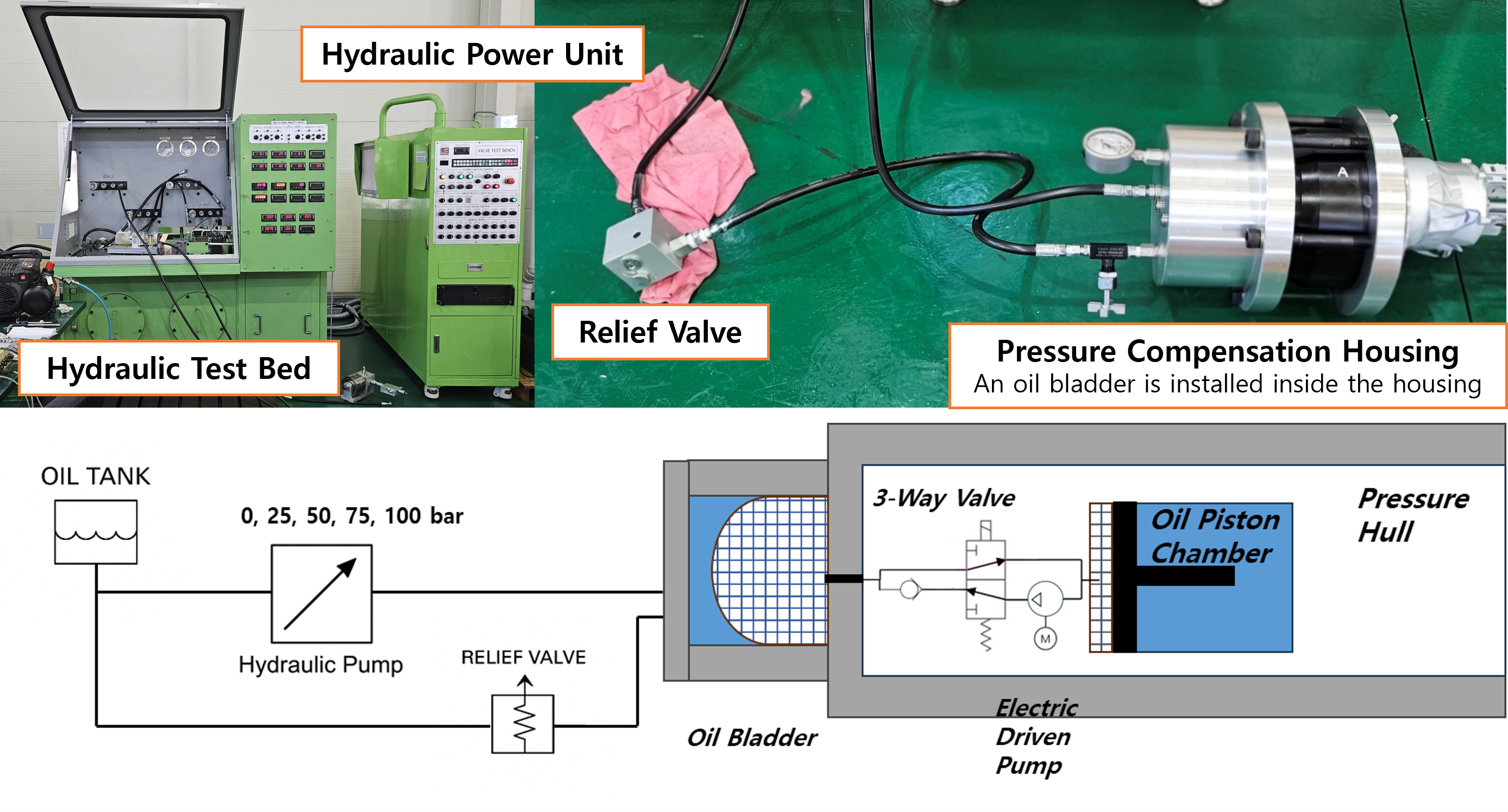
To characterize the buoyancy engine’s drive behavior, a dedicated test apparatus capable of replicating pressures up to 100 bar was constructed (Figure 5). A constant-pressure maintenance device and relief valve were incorporated to suppress pressure fluctuations induced by bladder inflation and maintain a stable back-pressure load throughout testing.

2.3.2. Quantitative Modeling of Electro-Hydraulic Drive Characteristics

To quantify the buoyancy engine’s power consumption, discharge time, pump rotational speed, and current draw were measured across PWM inputs of 20–80% and pressure loads of 0–100 bar. Full experimental data are provided in Appendix A, Table A1, Table A2 and Table A3.
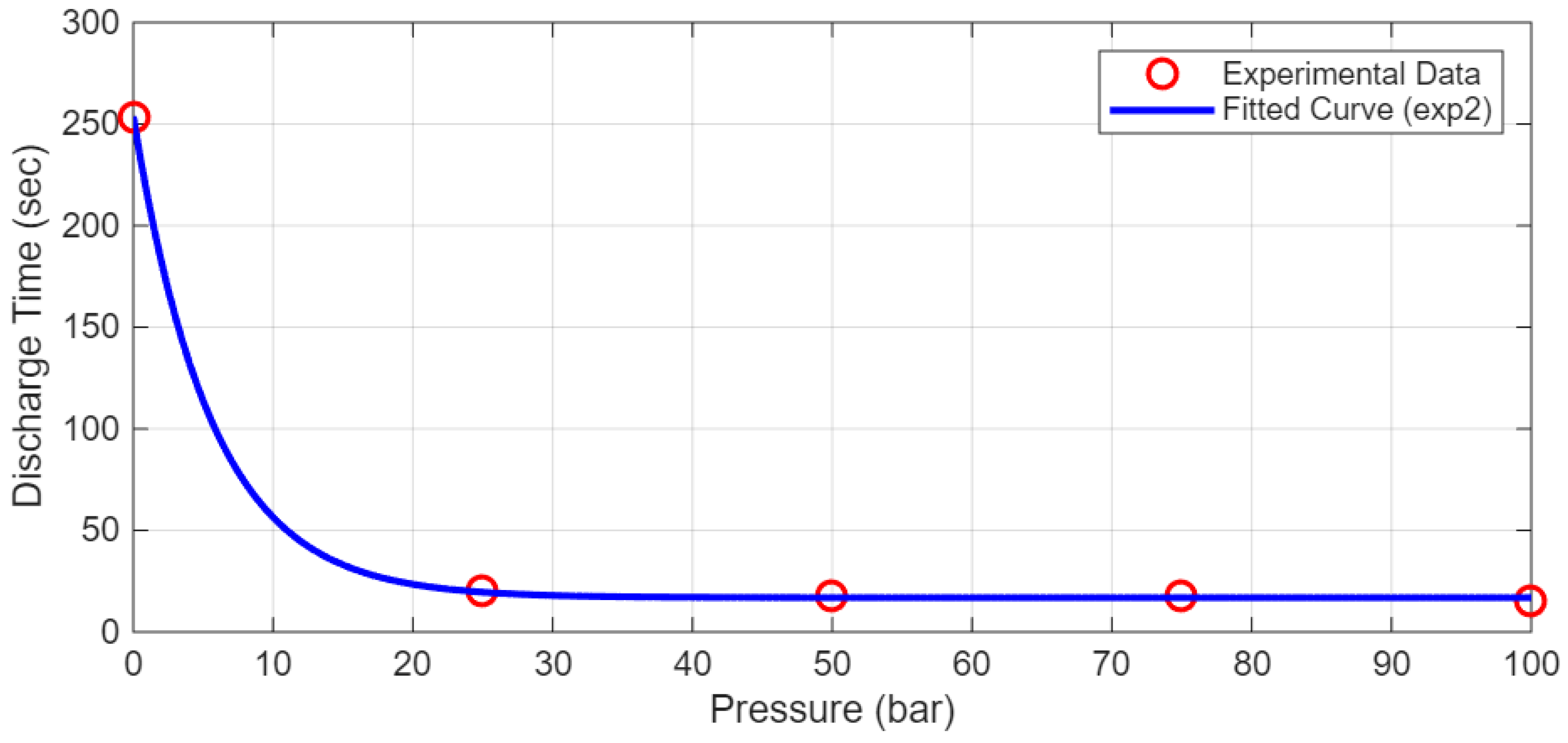
Discharge time as a function of pressure was fitted to a double exponential model, given as follows.
T p = 263.82 e 0.178 p + 16.88
The goodness of fit of the model was confirmed with R 2 = 0.9999, SSE = 2.7736, and RMSE = 0.7448, demonstrating that the model accurately reproduces the experimental data (Figure 6).
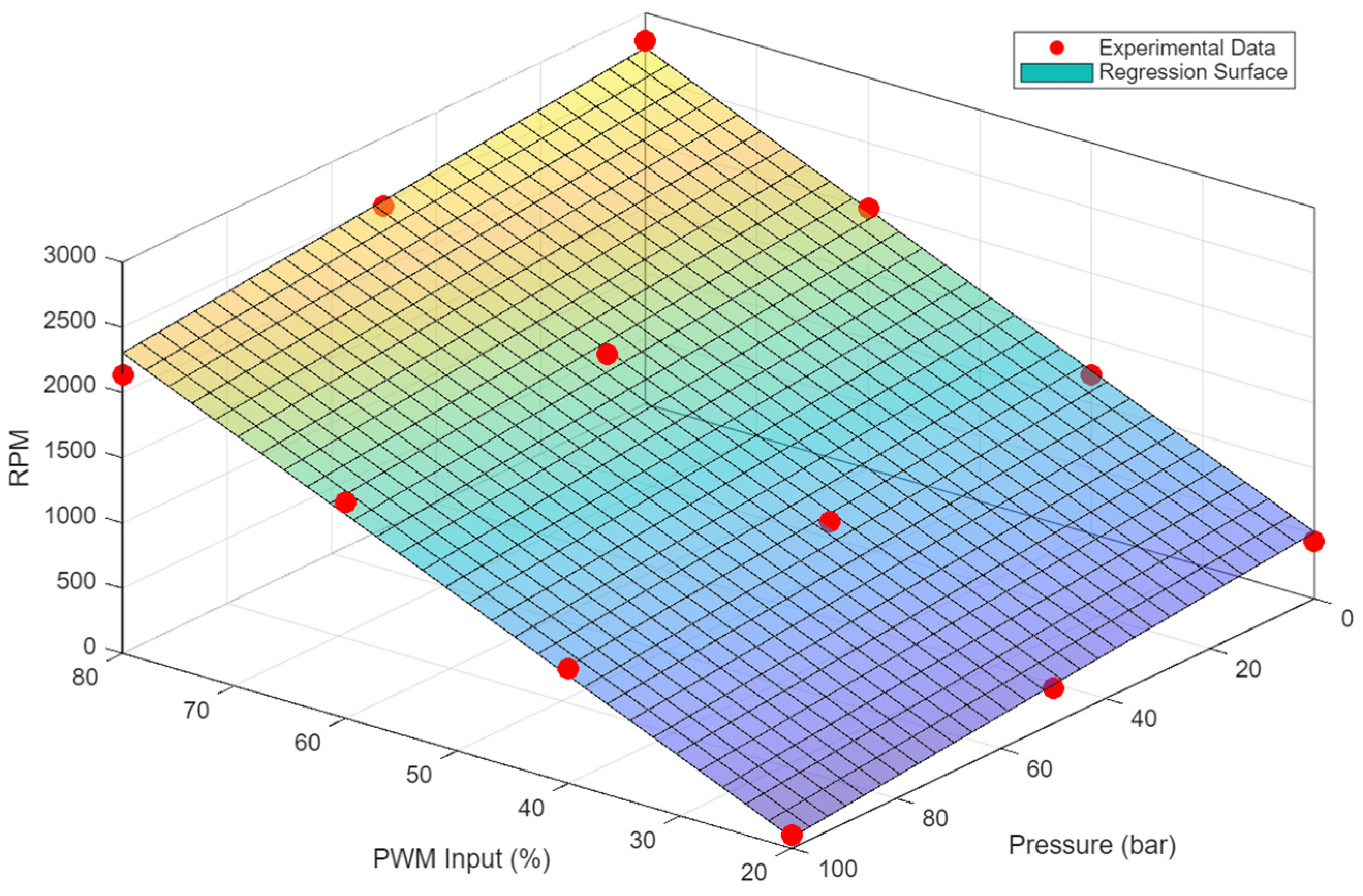
Pump rotational speed (RPM) was approximated using a two-variable linear regression model with PWM input and pressure as independent variables, as follows:
R P M u , p = 36.99 u 4.26 p 229.7
where u denotes the PWM input (%) and p denotes the pressure (bar). Since the pump used in the buoyancy engine (Breri, model akp105) has a displacement of 0.3 cc/rev, this model enables prediction of the hydraulic oil flow rate per unit time. The goodness of fit was confirmed with R 2 = 0.9937, RMSE = 66.81, and SSE = 53,570.68, demonstrating that the model accurately reproduces the experimental data (Figure 7).
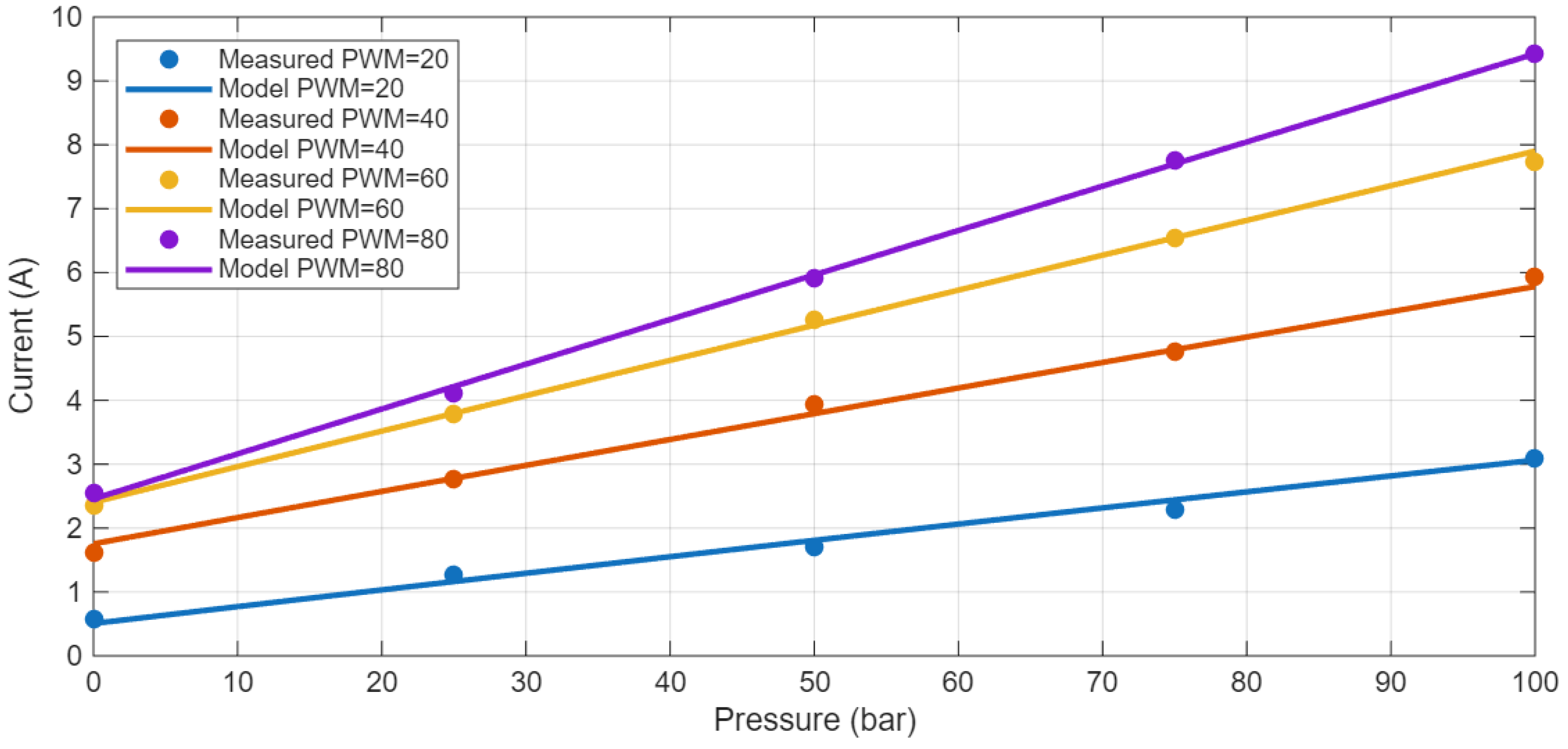
Current consumption of the buoyancy engine was similarly modeled as a second-order polynomial function of PWM input and pressure:
I ( p , u ) = ( 1.3388 + 1.072 × 10 1 u + 0.1465 p 0.000747 u 2 ) + ( 0.0118 + 7.35 × 10 4 u ) p   9.25 × 10 6 p 2
where I denotes the output current ( A ), u denotes the PWM input (%), and p denotes the pressure (bar). The goodness of fit was confirmed with R 2 = 0.9985, RMSE = 0.0918 A, and SSE = 0.1685, demonstrating that the model accurately reproduces the experimental data (Figure 8).

2.3.3. Attitude Controller Power Consumption Modeling

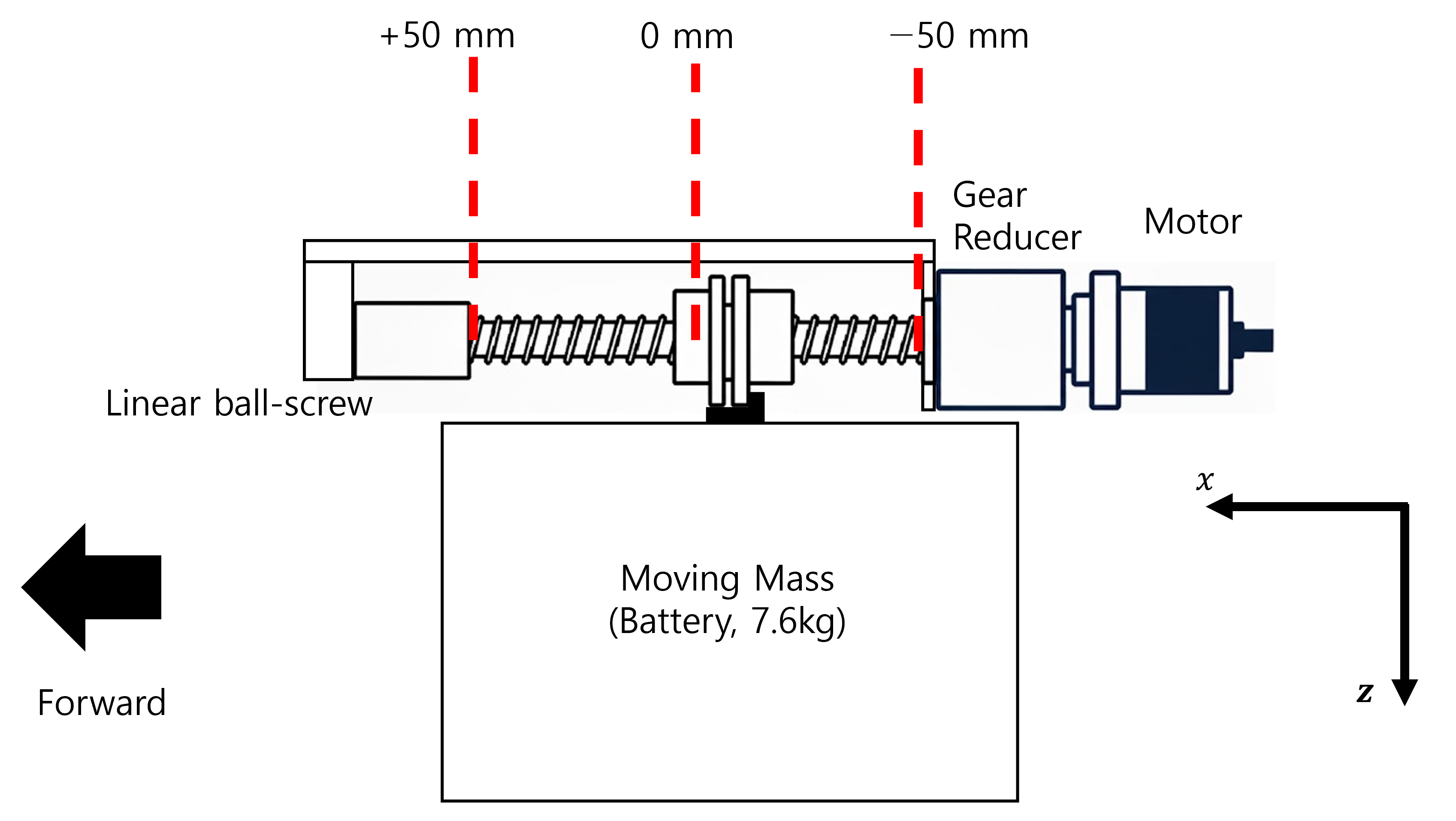
The attitude controller is driven by a Maxon RE25-339150 DC motor (12 V, 20 W) coupled to a GP26A-406762 planetary gearhead with a 19:1 reduction ratio. Pitch angle is regulated by translating a 7.6 kg battery pack along the hull’s longitudinal axis via a ball screw mechanism, shifting the center of gravity accordingly (Figure 9). The battery travels within a ±50 mm range referenced to the hull centerline, with forward displacement defined as positive and rearward as negative. Position is continuously monitored by a MEGATRON MBX-150 linear potentiometer with a sensing stroke of 150 ± 0.3 mm.
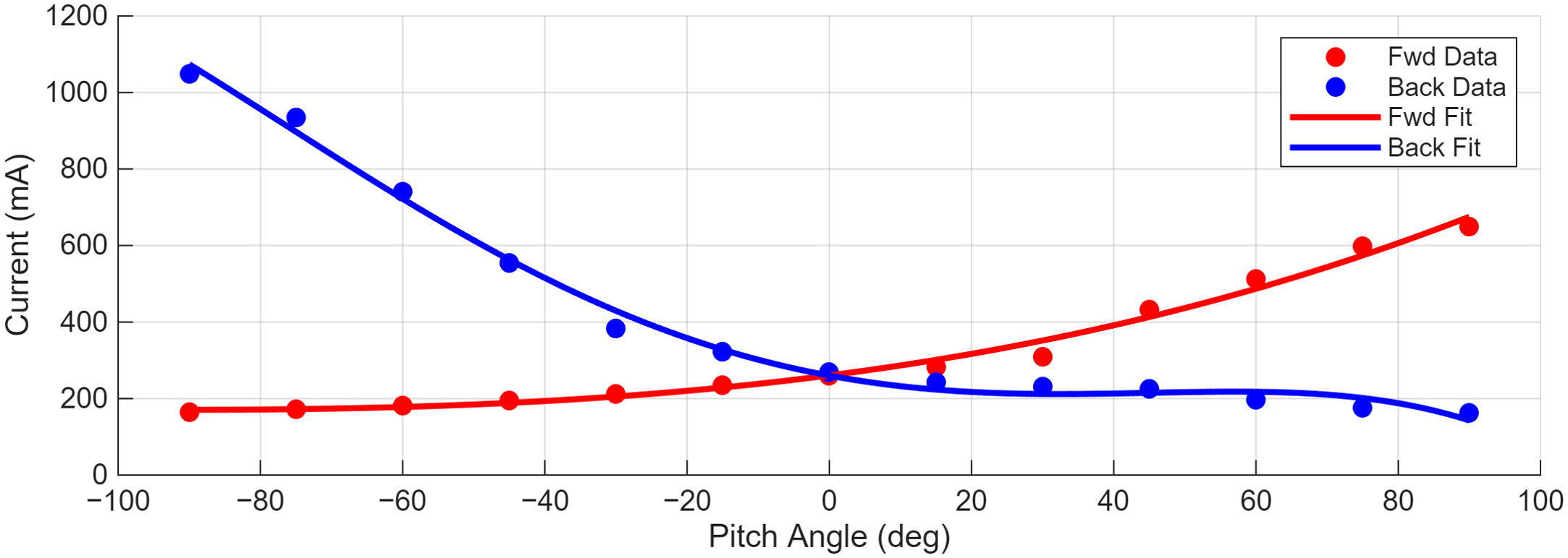
To characterize the attitude controller’s power consumption, current draw was measured on the fully assembled glider across pitch angles from −90° to +90° in 15° increments. Separate measurements were taken for forward and backward battery displacement, as current consumption differs between the two directions. Mean values from 10 repeated trials are listed in Table 3
Forward and backward battery displacement were modeled separately, yielding a third-order polynomial for the forward direction and a fourth-order polynomial for the backward direction.
I f w d ( θ ) = ( 5.0514 × 10 5 ) θ 3 + ( 2.006 × 10 2 ) θ 2 + 2.394 θ + 260.4189   I b a c k θ = 3.4088 × 10 6 θ 4 + 2.1455 × 10 4 θ 3   + 7.0622 × 10 2 θ 2 3.433 θ + 268.3
In the equations, θ denotes the pitch angle (degrees), and I f w d and I b a c k denote the current consumption (mA) during forward and backward battery displacement, respectively. Both models showed strong agreement with the experimental data: the forward model achieved R 2 = 0.9867, RMSE = 18.620 mA, and SSE = 4506.937, and the backward model achieved R 2 = 0.9935, RMSE = 23.463 mA, and SSE = 7156.731.
Figure 10 compares the measured current consumption against both fitted models across the full range of pitch angles.

3. Intelligent Pitch Control System Design

The glider’s drive system comprises three subsystems: a buoyancy controller, an attitude controller, and a heading controller. While reducing buoyancy variation lowers energy consumption, East Sea operations impose a minimum forward speed requirement of 0.7 knots [3]. Hong et al. [3] report that peak horizontal speed is achieved at a pitch angle of ±35°, with forward speeds above 0.7 knots attainable when buoyancy exceeds 0.5% of the displaced volume. Although the glider in this study differs in hull geometry and hydrodynamic characteristics from that of [3], simulations conducted at a buoyancy control volume of ±300 cc and a desired pitch angle of ±35° yielded a minimum forward speed of 0.83 knots, confirming compliance with East Sea operational requirements. A fixed buoyancy control volume of ±300 cc was therefore adopted throughout this study.
Unlike the buoyancy controller, the attitude controller must continuously reposition the internal moving mass to hold the desired pitch angle, making it a prime candidate for energy saving through smarter control design. With buoyancy conditions fixed, this study focuses on developing an intelligent pitch control algorithm that minimizes unnecessary actuator motion and reduces the overall energy burden of the attitude controller.

3.1. PID Controller Design

As a reference for comparison, pitch angle control was first implemented using a conventional PID controller, whose control law takes the form:
u p ( t ) = K p e θ ( t ) + K i e θ ( t ) d t + K d d e θ ( t ) d t
e θ ( t ) = θ d ( t ) θ ( t )
where K p ,     K i and K d are the proportional, integral, and derivative gains, and θ d and θ are the desired and current pitch angles, respectively. The gains were determined through simulation-based tuning as K p = 1, K i = 0.01 and K d = 1, achieving reliable pitch angle tracking, and the same gains were applied to the sea trial experiments. The simulation sampling time was 0.1 s, and the battery position actuator limit of ±50 mm was enforced through a saturation block.
While the PID controller is straightforward to implement and provides a stable performance baseline, its fixed-gain nature makes it poorly suited to the nonlinear and time-varying conditions encountered during underwater glider operation. Of particular concern is the tendency for continuous error-driven corrections to repeatedly actuate the moving mass even after pitch convergence, unnecessarily burdening the attitude controller with avoidable energy losses. These shortcomings motivate the development of the fuzzy and ANFIS-based fuzzy controllers presented in the sections that follow.

3.2. Sugeno-Type Fuzzy Controller Design

A Sugeno-type Fuzzy Inference System (FIS) was designed to determine the optimal battery position, taking pitch angle error, desired pitch angle, and buoyancy control volume as inputs. The Sugeno-type FIS expresses the consequent as a linear function, which offers the advantages of computationally efficient defuzzification and suitability for real-time implementation [22].
The fuzzy controller comprises three input variables. The first input is the pitch angle error e θ , partitioned into five linguistic variables, namely NB, NS, ZO, PS, and PB, with trapezoidal and triangular membership functions applied. The second input is the desired pitch angle θ d , categorized into three modes, namely DIVE, ZERO, and RISE, to identify the motion phase of the glider. The third input is the buoyancy control volume (200–500 cc), defined with a single membership function, namely ACTIVE, to reflect the active state of the buoyancy engine. The output is the battery position (mm), represented by nine linear consequent functions.
The rationale for incorporating the buoyancy control volume as the third input is as follows. As the buoyancy control volume increases, the pitch angle of the underwater glider increases correspondingly, and the battery displacement required to maintain a given pitch angle decreases linearly. This relationship was incorporated into the linear consequent functions to enable linear compensation of battery position in response to variations in buoyancy control volume.
The consequent was designed in three regions according to the motion mode. In the DIVE and RISE regions, the battery position was expressed as a linear function proportional to the desired pitch angle and buoyancy control volume. A sequentially decreasing structure was applied, in which the battery displacement increases with larger errors and decreases monotonically as the error approaches ZO.
In the ZERO region, to suppress hunting behavior, in which the pitch angle fluctuates again due to moving mass inertia after convergence to the desired pitch angle, the battery position was fixed at its current location by setting f 5 = 0 upon entry into the ZO zone. This design accounts for the characteristically slow dynamic response of underwater gliders and effectively eliminates unnecessary actuator motion after convergence, thereby reducing energy consumption.
The rule base comprises a total of 13 If-Then rules, as listed in Table 4. The product method was applied for the AND operation, and the weighted average method was applied for defuzzification.
Two notable aspects of the rule-based design warrant attention. First, in the DIVE mode, the same consequent f 3 was applied when the error was ZO, PS, or PB. This was intended to maintain the current control state without additional battery displacement when the error became sufficiently small during descent. Second, in the RISE mode, the same consequent f 7 was applied for errors of NB, NS, and ZO, for the same reason, namely to suppress unnecessary actuator motion in the low-error region during ascent. Third, in the ZERO mode, the NS and PS rules were omitted, with only NB, ZO, and PB defined. This simplifies the error response in the horizontal phase and explicitly enforces the neutral condition of fixing the battery position upon entry into the ZO zone, expressed as f 5 = 0.
The 13 rules share 9 unique consequent functions ( f 1 through f 9 ), as multiple rules in the DIVE and RISE modes map to the same consequent (e.g., DIVE-ZO, DIVE-PS, and DIVE-PB all map to f 3 ; RISE-NB, RISE-NS, and RISE-ZO all map to f 7 ). The coefficients of these 9 consequent functions, designed based on physical insight, are summarized in Table 5.

3.3. ANFIS-Based Fuzzy Controller Design

The Sugeno-type FIS developed in the previous section relied entirely on expert knowledge to define the rule structure and consequent parameters. While this approach captures domain insight effectively, manually tuned membership functions are inherently limited by designer experience and offer no guarantee of optimal control performance. To overcome this, ANFIS (Adaptive Neuro-Fuzzy Inference System) was employed to refine the membership function parameters through data-driven learning.
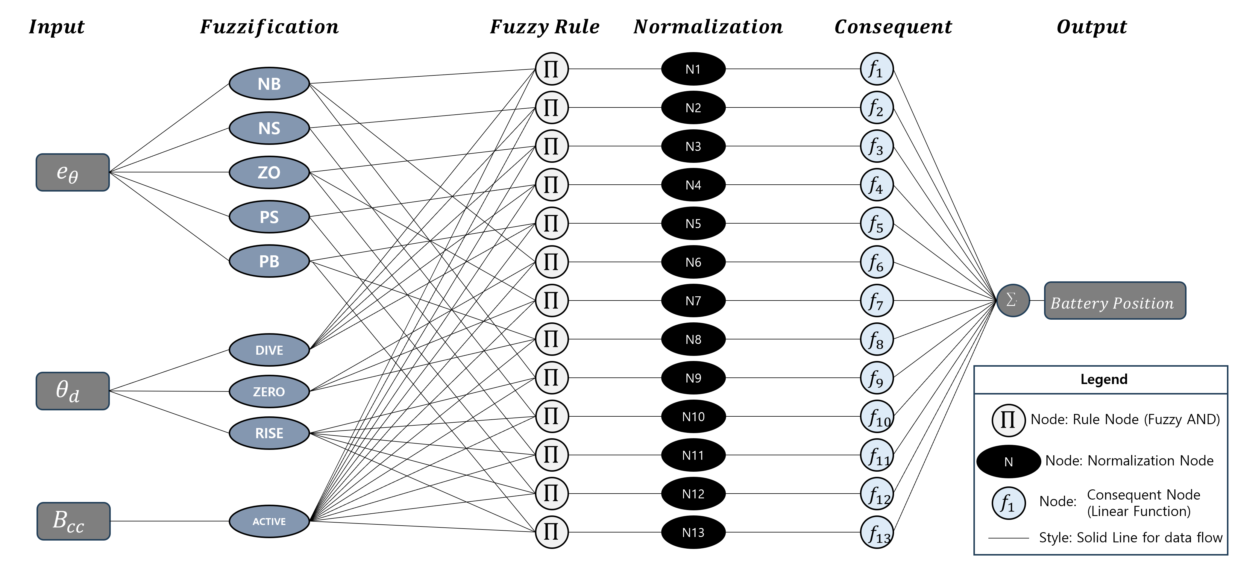
Introduced by Jang (1993) [18], ANFIS embeds the learning capability of neural networks within a fuzzy inference framework. Each network layer maps directly to a stage of the fuzzy inference process, namely fuzzification, rule operation, normalization, consequent evaluation, and defuzzification. A hybrid learning algorithm combining backpropagation and least squares estimation (LSE) simultaneously optimizes the premise parameters of the membership functions and the linear coefficients of the consequent, while leaving the expert-designed rule structure intact.
The training strategy is built around a simple but effective idea: use the battery positions that minimize energy consumption as target outputs. The converged battery position under PID corresponds to the moment equilibrium required to hold the desired pitch angle, representing the location at which no further actuation is needed to maintain the target attitude. The residual energy consumption observed in PID operation therefore arises from transient-error-driven corrections around this equilibrium, not from the equilibrium itself. Hence, these steady-state positions can be directly defined as the optimal target outputs for the data-driven learning framework. To capture the energy-optimal battery positions, steady-state convergence data were collected across buoyancy control volumes of 200–500 cc (in 100 cc increments) and desired pitch angles of −40° to +40° (in 10° increments), and organized into a one-dimensional lookup table. The resulting training dataset contains approximately 5500 samples.
The FIS structure takes three inputs: pitch angle error e θ (five membership functions), desired pitch angle θ d (three membership functions), and buoyancy control volume B c c (one trapezoidal membership function). The output, battery position, is represented as a linear consequent function. Training was carried out using the hybrid method over 30 epochs. The resulting ANFIS architecture is illustrated in Figure 11.
In this study, ANFIS is used not as a predictive model for unseen data, but to approximate a deterministic control map derived from the PID steady-state convergence results. Since the input domain of the training data coincides with the operational domain, all training samples were used without separate validation or testing partitions. The hybrid learning yielded a converged training RMSE of 1.38 × 10⁻⁴ m (≈0.138 mm), corresponding to approximately 0.14% of the actuator stroke range (±50 mm). The complete membership function parameters before and after ANFIS training are provided in Appendix A (Table A4, Table A5 and Table A6).
The proposed ANFIS controller is designed for operation within the training data domain (desired pitch angles of −40° to +40° and buoyancy control volumes of 200–500 cc). For inputs beyond this domain, the learned control map operates in an extrapolated region, and output oscillations may occur near the boundaries of the membership functions. The operating envelope of the controller is therefore confined to the training domain, and its extension through training dataset augmentation is addressed in Section 6.2.
After ANFIS training, the consequent function coefficients in Table 5 were optimized through hybrid learning. The trained consequent functions are summarized in Table 6. Notably, the three ZERO-region consequent functions ( f 4 ,   f 5 ,   f 6 ) all converged to zero after training, whereas only f 5 was set to zero in the initial design. This indicates that the learning naturally identified the neutral battery position as the energy-optimal solution under horizontal-hold conditions, consistent with the hunting suppression design intent stated in Section 3.2.

4. Simulation and Result Analysis

4.1. Simulation Environment Setup

A MATLAB/Simulink R2025b (MathWorks Inc., Natick, MA, USA)-based underwater glider simulator was developed by integrating the 6-DOF dynamic model, buoyancy-mass motion model, and experimentally derived actuator power models. The simulator takes the upper and lower depth bounds, desired pitch angle, and buoyancy control volume as inputs, and returns the glider’s velocity, position, actuator displacement, and power consumption. Simulation conditions are summarized in Table 7.

4.2. Performance Analysis by Controller

Three controllers were evaluated under identical simulation conditions: the PID controller, the manually designed Sugeno fuzzy controller, and the ANFIS-based fuzzy controller. The comparison focused on two key metrics: attitude tracking performance and energy consumption reduction.

4.2.1. Gliding Motion Performance Comparison

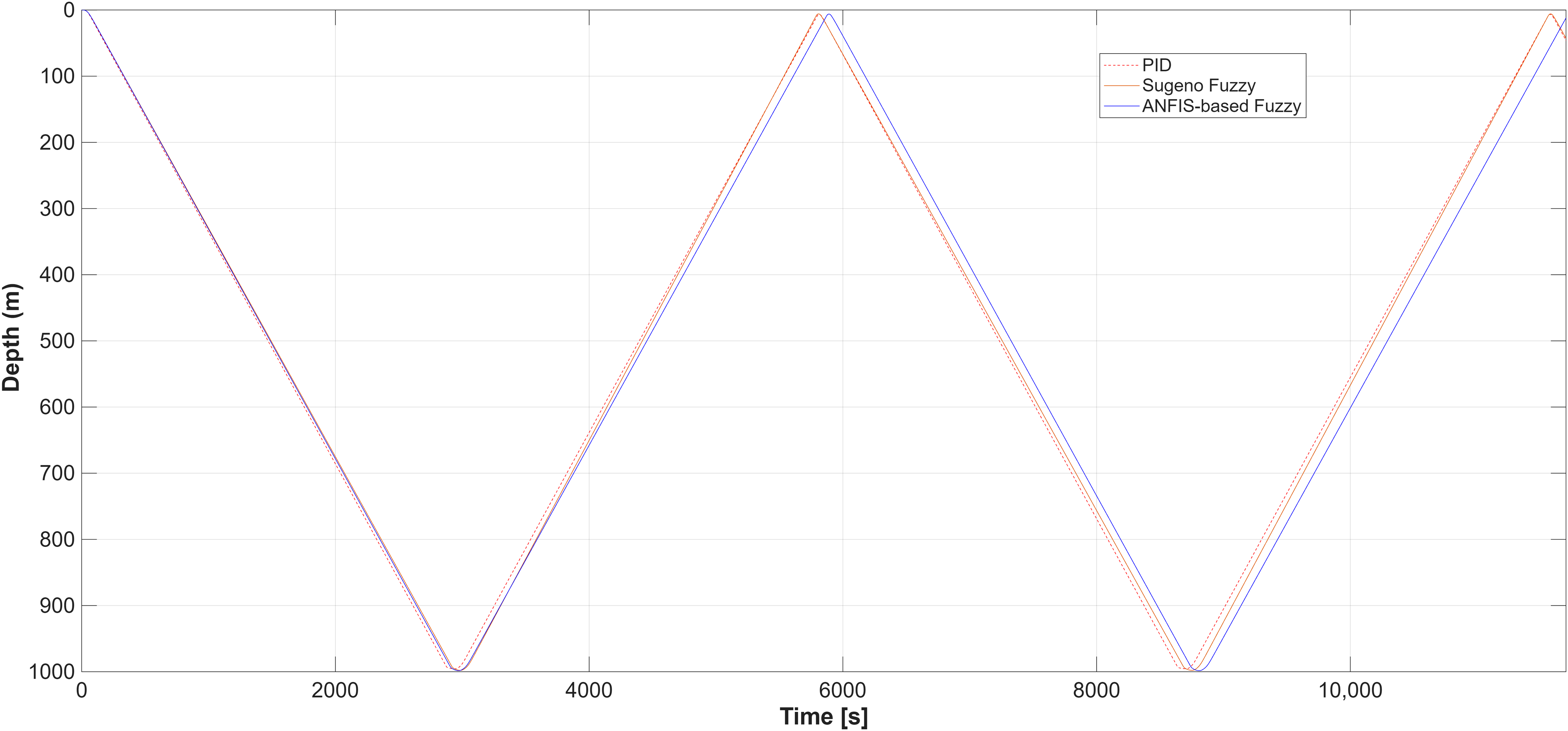
Figure 12 shows the depth and pitch angle responses of the three controllers over one complete dive-and-rise cycle (10–1000 m). The ANFIS-based fuzzy controller achieved the greatest horizontal travel distance at 4994.66 m, compared to 4912.2 m for both the PID and Sugeno fuzzy controllers. The 82.46 m gain (1.67%) is attributed to the improved pitch angle convergence characteristics of the ANFIS-based controller, which allowed the glider to maintain a more consistent glide path throughout the cycle.
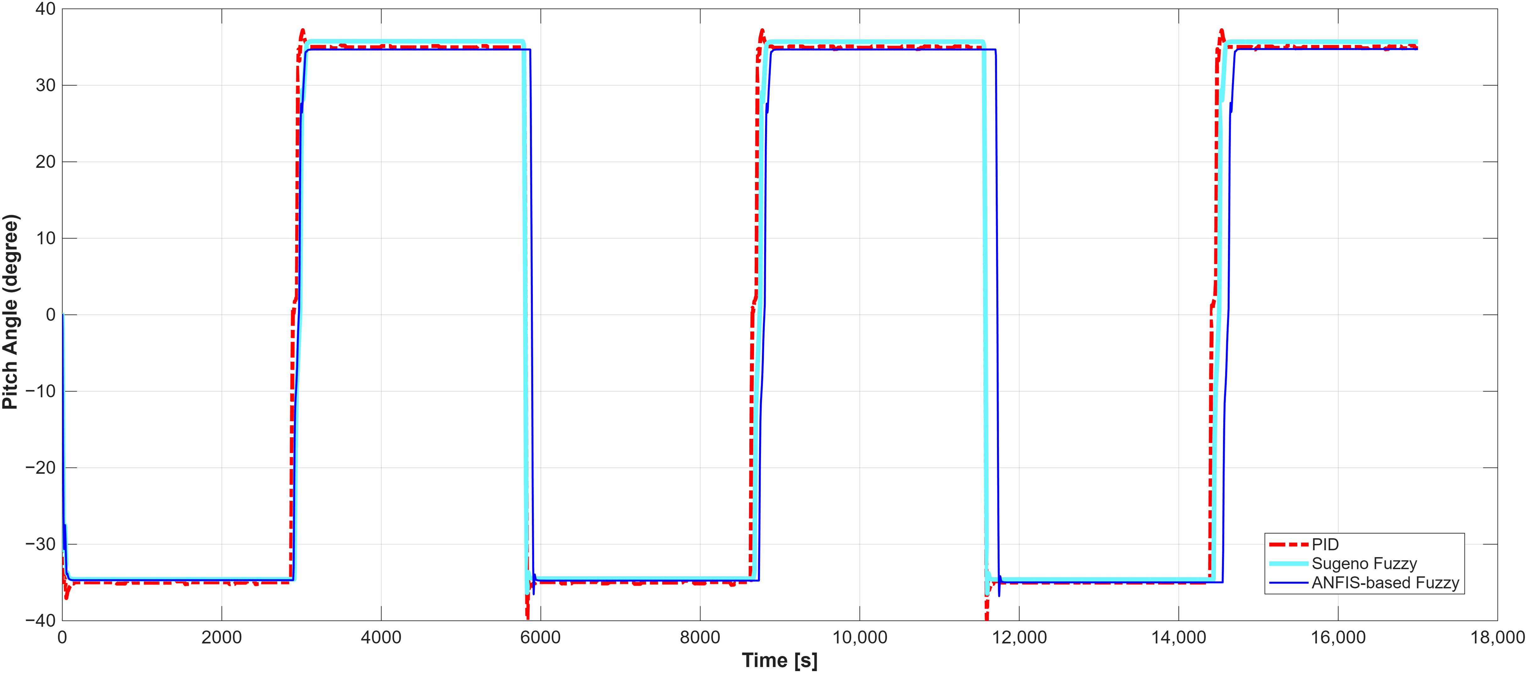
Figure 13 compares the pitch angle tracking performance of all three controllers. The PID controller overshot by 1.47° at +35° and by 4.49° at −35°, with the asymmetry likely reflecting the difference in nonlinear buoyancy forces between the ascending and descending phases. Both the Sugeno fuzzy and ANFIS-based fuzzy controllers overshot by roughly 1.3° during the −35° phase before settling cleanly, and converged without overshoot at +35°, outperforming PID in transient response.
In steady state, the Sugeno fuzzy controller retained a residual offset of around 0.7°, while both the PID and ANFIS-based fuzzy controllers held within approximately 0.1°. The larger offset of the Sugeno fuzzy controller stems from the limitations of manual membership function tuning, which cannot fully capture the nonlinear input–output relationships of the system. The ANFIS-based fuzzy controller, whose membership functions were refined through data-driven learning, matched the steady-state accuracy of PID while retaining the interpretable rule structure of the underlying fuzzy inference system.

4.2.2. Battery Position Response Analysis

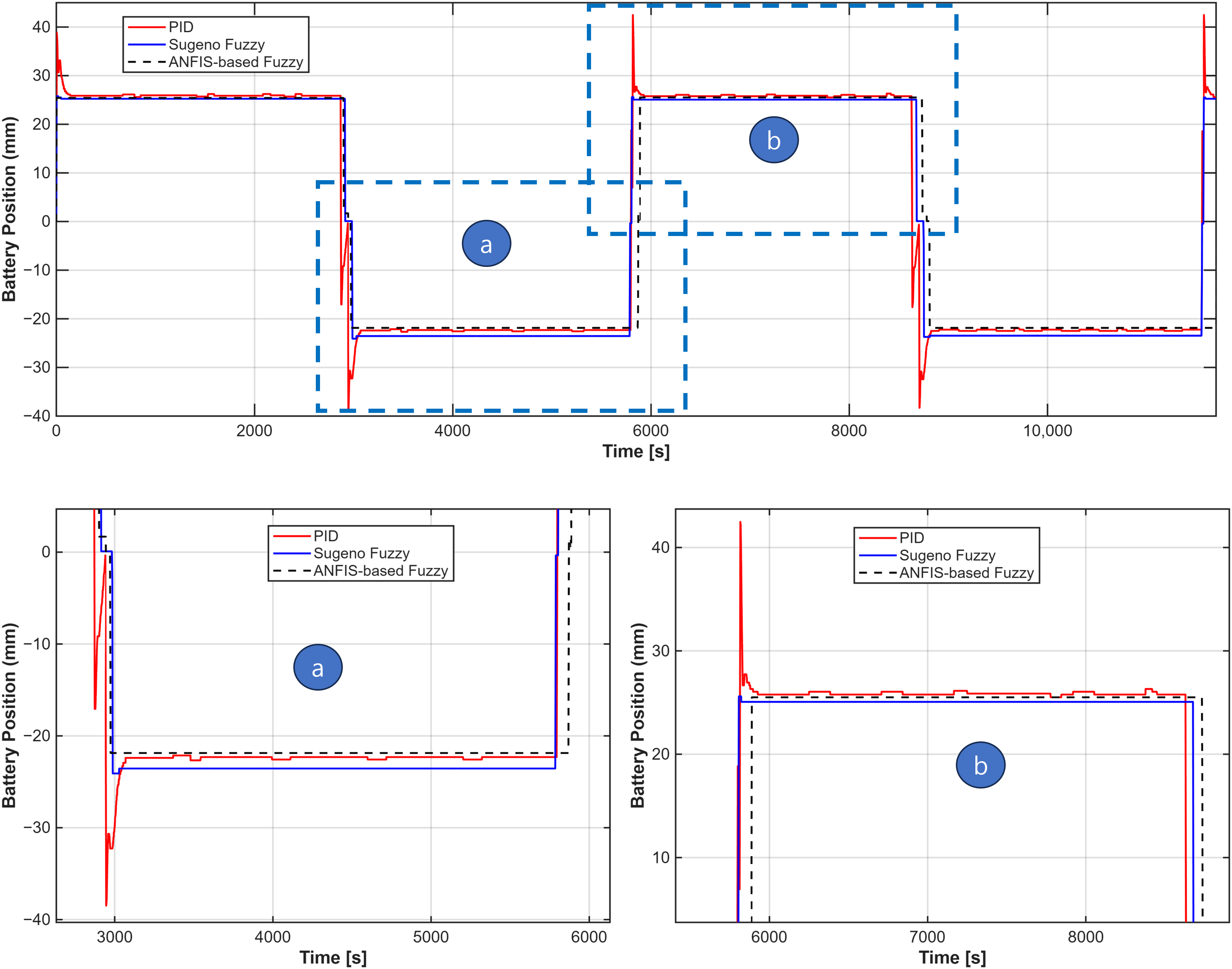
As shown in Figure 14, the PID controller produced noticeable battery overshoot whenever the pitch angle error was large. The Sugeno fuzzy controller settled at a position approximately 6.4 mm offset from that of the PID controller, but showed a clear tendency to limit battery movement after convergence. The ANFIS-based fuzzy controller, by contrast, drove the battery directly to the target position and held it there without further actuation. This behavior reflects the ability of ANFIS training to tune the membership functions to the inherently slow dynamics of the underwater glider, effectively eliminating the residual corrections that drive unnecessary actuator activity in the other two controllers.

4.2.3. Energy Consumption Analysis

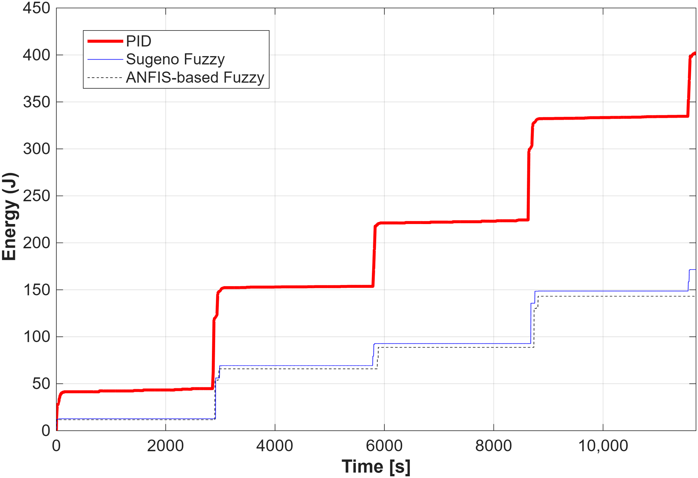
Table 8 and Figure 15 summarize the attitude controller energy consumption over one complete dive-and-rise cycle (10–1000 m) for each of the three controllers.
The ANFIS-based fuzzy controller reduced attitude controller energy consumption by 57.05% relative to PID and by 4.98% relative to the Sugeno fuzzy controller. While the per-cycle attitude controller energy consumption (65.876 J for the ANFIS-based fuzzy controller) accounts for only about 1.04% of the buoyancy engine energy consumption (6333.9 J per dive-and-rise cycle at ±300 cc buoyancy control), its impact accumulates significantly over extended deployments. With approximately 878 cycles completed over two months of continuous operation, switching from PID to the proposed controller is projected to save a cumulative 76,825 J, a meaningful gain for missions where every joule counts.

5. Algorithm Validation Through Sea Trial Experiments

5.1. Experimental Environment and System Configuration

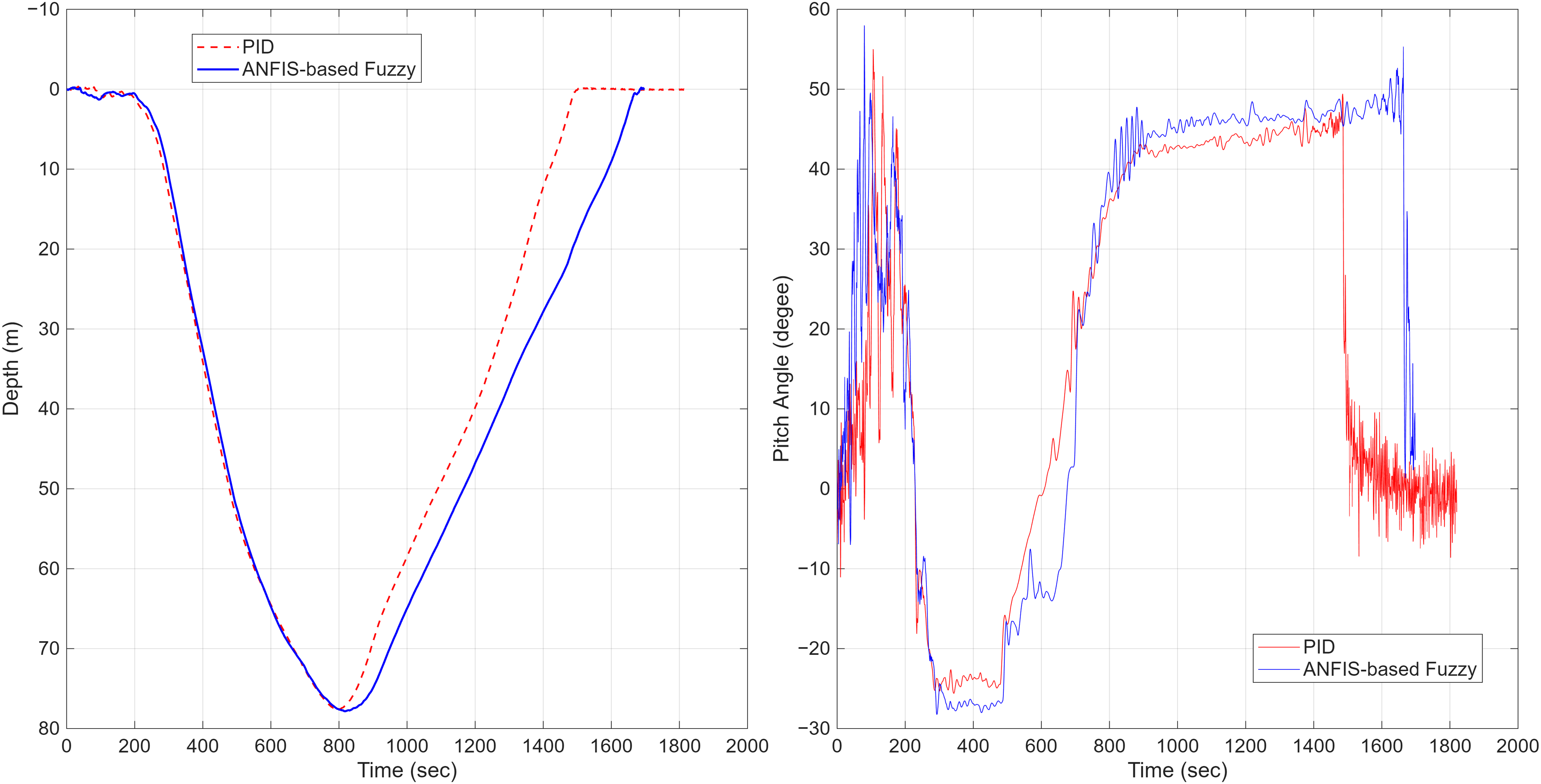
The target depth of the sea trial experiments was restricted to 50 m due to the safety line configuration and the site water depth, which differs from the 1000 m simulation conditions. Consequently, the sea trial experiments primarily validate the qualitative behavior of the proposed controller, specifically the reduction in moving mass displacement, rather than the energy reduction effect reported in simulation. Long-term performance testing under free-running conditions without the safety line is planned as future work to quantitatively verify the energy reduction effect.
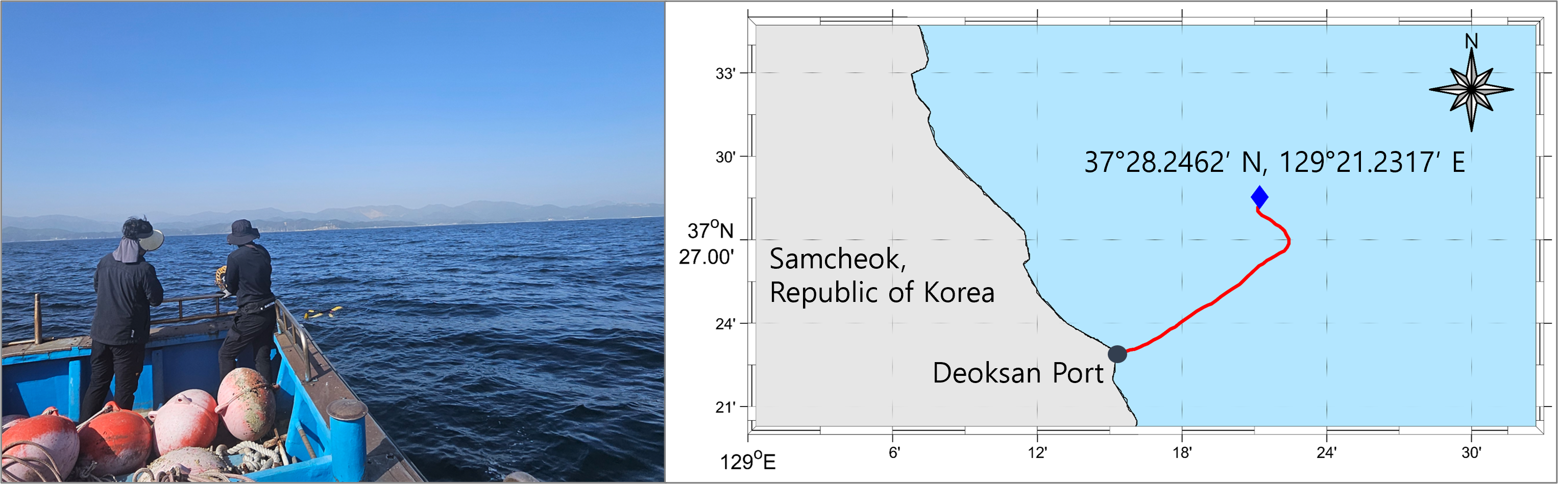
Sea trial experiments were carried out on 20–21 April 2026, in the coastal waters off Deoksan Port, Samcheok, Republic of Korea (37°28.2462′ N, 129°21.2317′ E), to directly compare the performance of the ANFIS-based fuzzy controller and the PID controller under real ocean conditions. At the time of the experiments, the water temperature was approximately 15 °C, significant wave height remained below 1.2 m, and peak wind gusts reached 12.1 m/s. The site water depth was approximately 200 m.
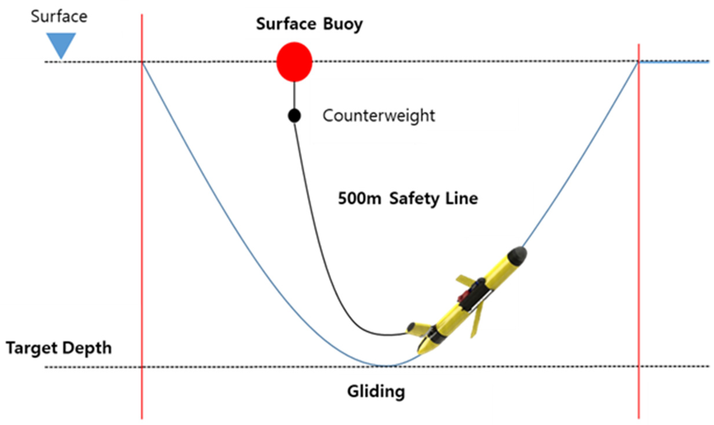
As the underwater glider is currently in the development stage, experiments were conducted with a 500 m safety line connected to the glider to ensure operational safety (Figure 16). Figure 17 illustrates the sea trial configuration, in which the underwater glider is connected to a surface buoy via a 500 m safety line with a counterweight to maintain tension, enabling safe recovery while allowing the glider to execute dive-and-rise cycles to the target depth. The experimental conditions were set as follows: target depth of 50 m, buoyancy control volume of ±300 cc, and desired pitch angle of ±35°. The PID controller gains were set to K p = 1, K i , = 0.01, K d = 1, identical to those used in the simulation.
In the present sea trial, one dive-and-rise cycle was performed for each controller, with the ANFIS-based fuzzy controller test conducted immediately after the PID test under the same safety line configuration to minimize environmental variation between the two controllers. The trial was conducted with a small fishing vessel, and cycle-level environmental data (wave height, wind speed) could not be recorded due to the absence of onboard measurement equipment; the environmental conditions reported above represent the overall range during the trial period. Statistical repeatability analysis was not performed due to the limited number of trials, and the present sea trial is intended to provide qualitative verification of the controller behavior at the prototype development stage.

5.2. Experimental Results and Discussion

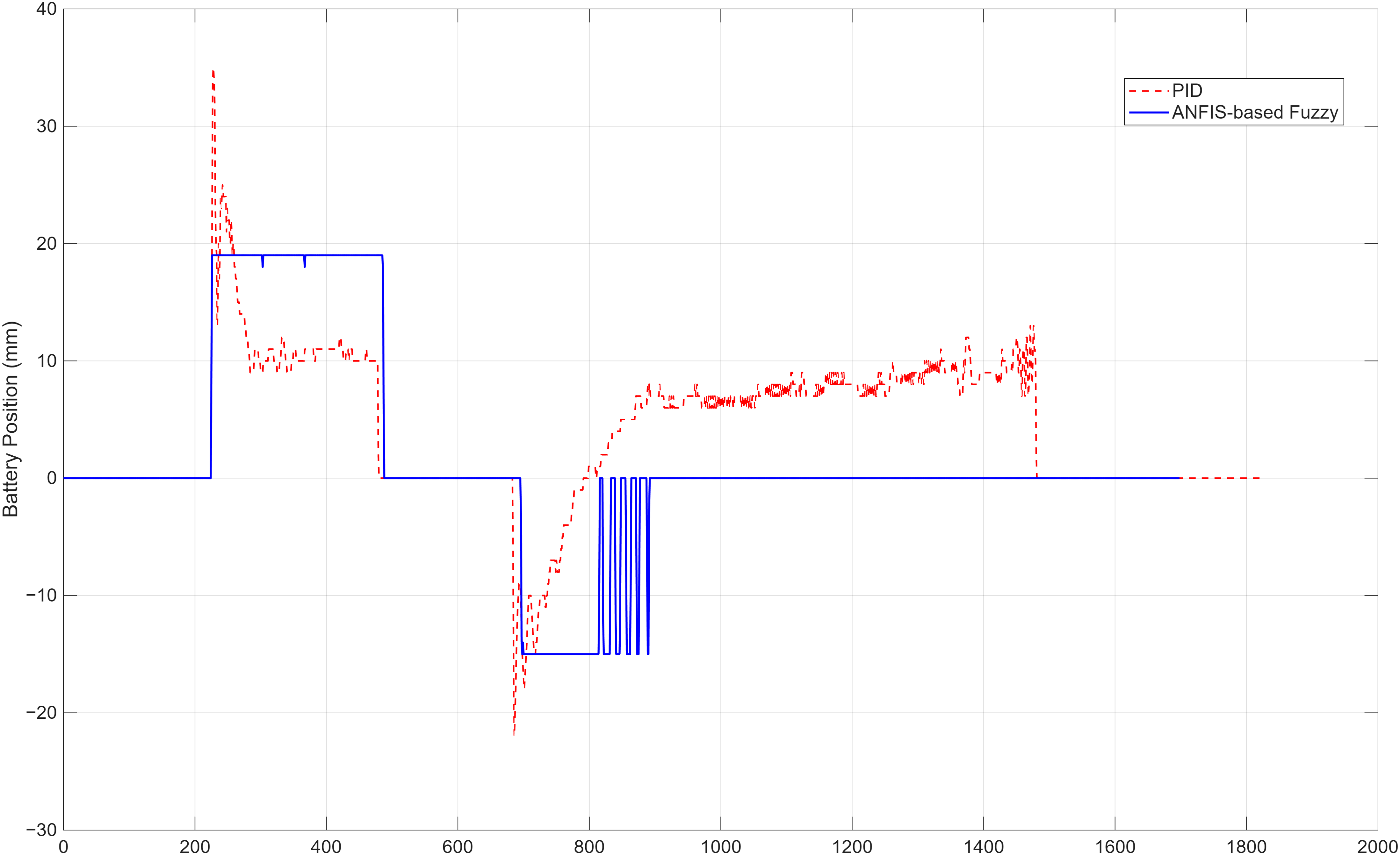
Figure 18 compares the depth and pitch angle responses of the PID and ANFIS-based fuzzy controllers during the sea trial. The safety line connecting the glider to the surface buoy introduced persistent external disturbances, which precluded a rigorous quantitative comparison of depth tracking performance. Despite this limitation, the battery position data in Figure 19 clearly reveal the behavioral differences between the two controllers. The PID controller drove the battery pack continuously throughout the entire trial, while the ANFIS-based fuzzy controller settled at the desired position early and held it steadily through both the diving and rising phases. These qualitative observations are consistent with the simulation results, indicating that the proposed controller suppresses unnecessary moving mass actuation under disturbance conditions. However, the safety line acted as a persistent external disturbance throughout the trial, and a full quantitative validation of the energy reduction effect could not be obtained from this sea trial.
However, during the sea trial, disturbances induced by the safety line caused the actual pitch angle to exceed the desired angle of 35°, reaching approximately 43.32°. In this case, as the pitch angle error e θ increased, a chattering phenomenon was observed in which the fuzzy output alternated repeatedly between 0 and 15 mm near the boundary of the NB membership function. This behavior corresponds to the operating envelope limitation noted in Section 3.3: the pitch angle (≈43.32°) exceeded the training data domain (±40°), causing the learned control map to operate in an extrapolated region near the membership function boundary. The chattering is therefore a manifestation of the explicit operating envelope limitation rather than a fundamental instability of the proposed method, and can be mitigated by extending the training dataset, as discussed in Section 6.2.

6. Conclusions

6.1. Summary of Research Outcomes

This study presented an intelligent pitch control algorithm for a 1000 m-class underwater glider, with performance validated through both simulation and sea trial experiments. The main findings are as follows.
First, a high-fidelity glider simulator was built by combining a nonlinear 6-DOF dynamic model with experimentally derived actuator power models, enabling simultaneous assessment of attitude stability and energy consumption.
Second, a 13-rule Sugeno-type fuzzy inference system was designed from physical insight, with membership function parameters subsequently refined through ANFIS training. The controller takes pitch angle error, desired pitch angle, and buoyancy control volume as inputs, and explicitly incorporates a neutral condition to eliminate unnecessary actuation once the pitch angle has converged.
Third, simulations showed that the proposed ANFIS-based fuzzy controller reduced attitude controller energy consumption by 57.05% relative to PID and by 4.98% relative to the manually tuned Sugeno fuzzy controller. Projected over two months of continuous operation, this translates to an estimated total energy saving of approximately 76,825 J against PID control.
Fourth, sea trials qualitatively confirmed that the ANFIS-based fuzzy controller exhibited substantially lower battery displacement than PID under disturbance conditions from the safety line. Over one complete dive-and-rise cycle, the PID controller accumulated a total battery travel distance of 512 mm (142 mm diving, 370 mm rising), while the ANFIS-based fuzzy controller recorded only 224 mm (42 mm diving, 182 mm rising), a reduction of 56.3%. These observations provide qualitative consistency with the simulation results, but should not be interpreted as a full quantitative validation of energy reduction

6.2. Future Research Directions

The limitations identified in this study and the directions for future research are as follows.
First, the safety line connected during the sea trial experiments acted as a disturbance, constraining the quantitative validation of depth tracking performance. Future work will involve long-term performance testing under free-running conditions without the safety line to quantitatively verify the energy reduction effect of the algorithm.
Second, chattering was observed when the pitch angle exceeded 43.32° during the sea trial experiments. To resolve this issue, it is necessary to expand the rule design range and training dataset, and to enhance control stability at boundary conditions.
Third, the power consumption models presented in this study were characterized under controlled hydrostatic pressure conditions. Extending these models to account for real-world oceanographic variability, including ambient currents and water temperature gradients, remains an important direction for future work and would further improve the predictive fidelity of the simulation framework.

Author Contributions

Conceptualization, S.-H.K.; methodology, S.-H.K., D.J. and H.C.; software, S.-H.K. and D.J.; validation, S.-H.K. and H.C.; formal analysis, S.-H.K.; investigation, J.-W.H. and S.-K.J.; resources, J.-W.H. and S.-K.J.; data curation, J.-W.H. and S.-K.J.; writing—original draft preparation, S.-H.K.; writing—review and editing, S.-H.K. and J.-Y.K.; visualization, S.-H.K.; supervision, J.-Y.K.; project administration, J.-Y.K.; funding acquisition, J.-Y.K. All authors have read and agreed to the published version of the manuscript.

Funding

This research was supported by the Unmanned Vehicles Core Technology Research and Development Program through the National Research Foundation of Korea (NRF) and the Unmanned Vehicle Advanced Research Center (UVARC), funded by the Ministry of Science and ICT, Republic of Korea (grant number NRF-2020M3C1C1A02086324). This research was also supported by the Korea Institute of Marine Science and Technology Promotion (KIMST), funded by the Korea Coast Guard (grant number RS-2021-KS211488). Additionally, this research was supported by the Korea Institute of Marine Science and Technology Promotion (KIMST), funded by the Ministry of Oceans and Fisheries, Republic of Korea (grant number RS-2024-00432366). The APC was funded by the National Research Foundation of Korea (grant number NRF-2020M3C1C1A02086324).

Data Availability Statement

The training dataset (approximately 5500 samples derived from PID steady-state convergence results) is available from the corresponding author upon reasonable request, subject to institutional approval.

Conflicts of Interest

The authors declare no conflicts of interest.

Appendix A

Table A1. Measured pump rotational speed (RPM) as a function of PWM input and pressure level (mean ± standard deviation of 10 trials).
PWM Input (%)Pressure (bar)RPM
Mean ± SD
200442 ± 2
50269 ± 1
10099 ± 1
4001223 ± 4
501050 ± 5
100878 ± 8
6002000 ± 8
501840 ± 10
1001655 ± 16
8002782 ± 9
502470 ± 14
1002140 ± 19
Table A2. Discharge time for 1000 cc oil transfer by the buoyancy engine at different pressure levels (mean ± standard deviation of 10 trials).
Pressure (bar)Discharge Time for 1000 cc (sec)
Mean ± SD
0253.70 ± 7.61
2520.00 ± 0.40
5017.73 ± 0.44
7517.39 ± 0.26
10015.59 ± 0.18
Table A3. Measured current consumption of the buoyancy engine as a function of pressure and PWM input level (mean ± standard deviation of 10 trials).
Pressure (bar)PWM = 20PWM = 40PWM = 60PWM = 80
Ampere
Mean ± SD
Ampere
Mean ± SD
Ampere
Mean ± SD
Ampere
Mean ± SD
00.5667 ± 0.00281.6210 ± 0.00772.3543 ± 0.01242.5581 ± 0.0148
251.2600 ± 0.00422.7733 ± 0.00993.7790 ± 0.01204.1190 ± 0.0156
501.7029 ± 0.00563.9343 ± 0.01455.2495 ± 0.02305.9124 ± 0.0325
752.2981 ± 0.01654.7619 ± 0.03286.5419 ± 0.04647.7486 ± 0.0581
1003.0952 ± 0.02905.9257 ± 0.05217.7286 ± 0.06029.4286 ± 0.0867
Table A4. Membership function parameters before and after ANFIS training (Input 1: Pitch angle error e θ   ( d e g ) ).
MFTypeBefore TrainingAfter Training
NBTrapmf[−90, −90, −86, −43][−129.3, −129.3, −86.12, −42.98]
NSTrimf[−65, −20, 0.2][−64.55, −21.4, 0.1693]
ZOTrimf[−7, 0 7][−7.022, 0.1693, 7.36]
PSTrimf[0.2, 22, 65][0.1693, 21.74, 64.89]
PBTrapmf[43, 86, 90, 90][43.32, 88.46, 129.6, 129.6]
Table A5. Membership function parameters before and after ANFIS training (Input 2: Desired pitch angle θ d (deg)).
MFTypeBefore TrainingAfter Training
DIVETrimf[−90, −45, −15][−70, −35, −5]
ZEROTrimf[−10, 0, 10][−10, 0, 10]
RISETrimf[15, 45, 90][5, 35, 70]
Table A6. Membership function parameters before and after ANFIS training (Input3: B c c   ( c c ) ).
MFTypeBefore TrainingAfter Training
ACTIVETrapmf[0, 0, 500, 500][0, 0, 500, 500]

References

  1. Stommel, H. The Slocum Mission. Oceanography 1989, 2, 22–25. [Google Scholar] [CrossRef]
  2. Purcell, M.; Bhatt, S.; Bhatt, M. Autonomous Underwater Glider: A Comprehensive Review. Drones 2025, 9, 21. [Google Scholar] [CrossRef]
  3. Hong, M.; Lee, S.; Hyeon, J.; Lee, J.; Lee, C.; Ko, S. Optimal Design of Combined Propulsion Underwater Glider for Operation of the East Sea of South Korea. Adv. Mech. Eng. 2019, 11, 1687814019856482. [Google Scholar] [CrossRef]
  4. Lan, W.; Jin, X.; Chang, X.; Wang, T.; Zhou, H.; Tian, W.; Zhou, L. Path Planning for Underwater Gliders in Time-Varying Ocean Current Using Deep Reinforcement Learning. Ocean Eng. 2022, 262, 112226. [Google Scholar] [CrossRef]
  5. Liu, Y.-H.; Su, Z.-Q.; Luan, X.; Song, D.-L.; Han, L. Motion Analysis and Fuzzy-PID Control Algorithm Designing for the Pitch Angle of an Underwater Glider. J. Math. Comput. Sci. 2017, 17, 133–147. [Google Scholar] [CrossRef]
  6. Zhao, W.; Guo, X.; Wang, Y. Attitude Control of Underwater Glider Combined Reinforcement Learning with Active Disturbance Rejection Control. J. Mar. Sci. Technol. 2019, 24, 686–704. [Google Scholar] [CrossRef]
  7. Wang, Z.; Yu, C.; Li, M.; Yao, B.; Lian, L. Vertical Profile Diving and Floating Motion Control of the Underwater Glider Based on Fuzzy Adaptive LADRC Algorithm. J. Mar. Sci. Eng. 2021, 9, 698. [Google Scholar] [CrossRef]
  8. Zhang, X.; Zhou, H.; Fu, J.; Wen, H.; Yao, B.; Lian, L. Adaptive Integral Terminal Sliding Mode Based Trajectory Tracking Control of Underwater Glider. Ocean Eng. 2023, 269, 113436. [Google Scholar] [CrossRef]
  9. Zhang, Z.; Wu, Y.; Zhou, Y.; Hu, D. Fault-Tolerant Control of Autonomous Underwater Vehicle Actuators Based on Takagi and Sugeno Fuzzy and Pseudo-Inverse Quadratic Programming under Constraints. Sensors 2024, 24, 3029. [Google Scholar] [CrossRef]
  10. Wang, P.; Wang, X.; Wang, Y.; Niu, W.; Yang, S.; Sun, C.; Luo, C. Dynamics Modeling and Analysis of an Underwater Glider with Dual-Eccentric Attitude Regulating Mechanism Using Dual Quaternions. J. Mar. Sci. Eng. 2023, 11, 5. [Google Scholar] [CrossRef]
  11. Ji, D.-H.; Lee, J.-H.; Ko, S.-H.; Hyeon, J.-W.; Lee, J.-H.; Choi, H.-S.; Jeong, S.-K. Design and Analysis of the High-Speed Underwater Glider with a Bladder-Type Buoyancy Engine. Appl. Sci. 2023, 13, 11367. [Google Scholar] [CrossRef]
  12. Lee, J.-M.; Choi, K.; Kim, T. Buoyancy-Engine Endurance Test by Use of Hydraulic Test Device. J. Ocean Eng. Technol. 2025, 39, 226–234. [Google Scholar] [CrossRef]
  13. Song, Y.; Ye, H.; Wang, Y.; Niu, W.; Wan, X.; Ma, W. Energy Consumption Modeling for Underwater Gliders Considering Ocean Currents and Seawater Density Variation. J. Mar. Sci. Eng. 2021, 9, 1164. [Google Scholar] [CrossRef]
  14. Cao, J.; Cao, M.; Wang, J.; Shi, Y. Motion Pattern Optimization and Energy Analysis for Underwater Glider Based on the Multi-Objective Artificial Bee Colony Method. J. Mar. Sci. Eng. 2021, 9, 327. [Google Scholar] [CrossRef]
  15. Wang, C.; Yang, M.; Wang, Y.; Ren, M.; Wang, Z.; Yang, S. Design and Optimization of Cylindrical Hull with Non-Uniform Arch Ribs for Underwater Gliders Based on Approximate Model and Experiments. Ocean Eng. 2022, 259, 111831. [Google Scholar] [CrossRef]
  16. Chen, J.; Wang, Y.; Wu, Z. Precise Underwater Gliders Pitch Control with the Presence of the Pycnocline. J. Mar. Sci. Eng. 2021, 9, 1013. [Google Scholar] [CrossRef]
  17. Leccese, F.; Cagnetti, M.; Giarnetti, S.; Petritoli, E.; Luisetto, I.; Tuti, S. A Simple Takagi-Sugeno Fuzzy Modelling Case Study for an Underwater Glider Control System. In Proceedings of the 2018 IEEE International Workshop on Metrology for the Sea; (MetroSea), Bari, Italy, 8–10 October 2018. [Google Scholar] [CrossRef]
  18. Jang, J.-S.R. ANFIS: Adaptive-Network-Based Fuzzy Inference System. IEEE Trans. Syst. Man. Cybern. 1993, 23, 665–685. [Google Scholar] [CrossRef]
  19. Santhakumar, M.; Asokan, T.; Kumar, A. Overshoot Reduction Using Adaptive Neuro-Fuzzy Inference System for an Autonomous Underwater Vehicle. Mathematics 2023, 11, 1868. [Google Scholar] [CrossRef]
  20. Alcala, E.; Puig, V.; Quevedo, J. Learning-Based Control of Autonomous Vehicles Using an Adaptive Neuro-Fuzzy Inference System and the Linear Matrix Inequality Approach. Sensors 2024, 24, 2551. [Google Scholar] [CrossRef]
  21. Fossen, T.I. Guidance and Control of Ocean Vehicles, 1st ed.; John Wiley & Sons: Chichester, UK, 1994; pp. 6–55. [Google Scholar]
  22. Takagi, T.; Sugeno, M. Fuzzy Identification of Systems and Its Applications to Modeling and Control. IEEE Trans. Syst. Man. Cybern. 1985, SMC-15, 116–132. [Google Scholar] [CrossRef]
  23. Graver, J.G. Underwater Gliders: Dynamics, Control and Design. Ph.D. Thesis, Princeton University, Princeton, NJ, USA, 2005. [Google Scholar]
  24. Huang, J.; Choi, H.-S.; Vu, M.T.; Jung, D.-W.; Choo, K.-B.; Cho, H.-J.; Nam Anh, P.H.; Zhang, R.; Park, J.-H.; Kim, J.-Y.; et al. Study on Position and Shape Effect of the Wings on Motion of Underwater Gliders. J. Mar. Sci. Eng. 2022, 10, 891. [Google Scholar] [CrossRef]
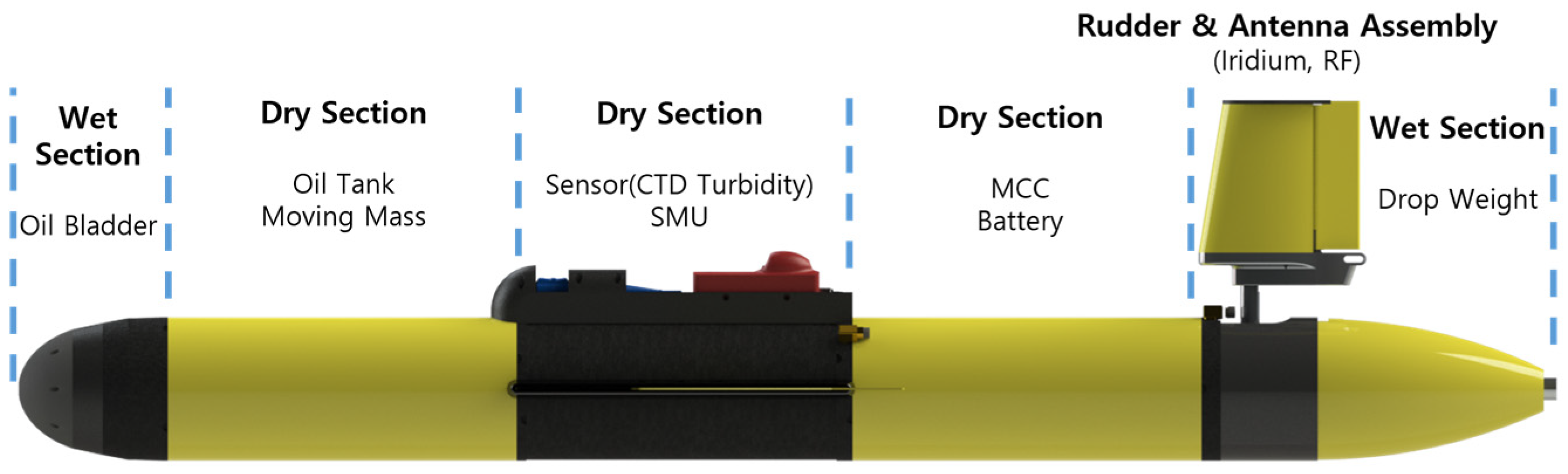
Figure 1. Photograph of the developed 1000 m-class underwater glider.
Jmse 14 00986 g001
Figure 2. Body-fixed and Earth-fixed coordinate systems defined for the underwater glider. The blue straight arrows indicate the linear velocities (u, v, w), and the green curved arrows indicate the angular velocities (p, q, r). The forces (Fx, Fy, Fz) and moments (Mx, My, Mz) are labeled in red text.
Jmse 14 00986 g002
Figure 3. Schematic diagram of the internal component layout showing position vectors of each mass element, serving as the geometric reference for computing the center of buoyancy and center of gravity.
Jmse 14 00986 g003
Figure 4. Hydraulic system configuration and operating principle of the buoyancy engine: (a) positive buoyancy generation via pump-driven oil discharge to the external bladder; (b) negative buoyancy generation via passive oil recovery driven by external hydrostatic pressure. The green arrow in (a) indicates the oil discharge flow direction during positive buoyancy generation, and the red arrow in (b) indicates the oil recovery flow direction during negative buoyancy generation.
Jmse 14 00986 g004
Figure 5. Experimental setup for buoyancy engine power consumption modeling: (Top-left) pressurized hydraulic test environment; (Top-right) pressure compensation system with internal oil bladder; (Bottom) schematic diagram of the power consumption measurement circuit.
Jmse 14 00986 g005
Figure 6. Discharge time as a function of pressure: comparison between measured data and the fitted double exponential model.
Jmse 14 00986 g006
Figure 7. Pump rotational speed (RPM) as a function of PWM input and pressure: comparison between experimental data and the two-variable linear regression model.
Jmse 14 00986 g007
Figure 8. Current consumption of the buoyancy engine as a function of PWM input and pressure: comparison between experimental data and the second-order polynomial regression model.
Jmse 14 00986 g008
Figure 9. Schematic diagram of the ball-screw-driven attitude control system: battery position is defined as 0 mm at the hull centerline, +50 mm toward the bow, and −50 mm toward the stern.
Jmse 14 00986 g009
Figure 10. Current consumption of the attitude controller as a function of pitch angle: comparison between measured data and fitted models for forward and backward battery displacement.
Jmse 14 00986 g010
Figure 11. ANFIS network structure of the proposed pitch controller: input layer, fuzzification layer, rule layer ( Π ), normalization layer (N), consequent layer ( f i ), and output layer ( Σ ).
Jmse 14 00986 g011
Figure 12. Depth profiles over time for PID, Sugeno Fuzzy, and ANFIS-Based Fuzzy controllers (desired depth: 10–1000 m, buoyancy control volume: ±300 cc).
Jmse 14 00986 g012
Figure 13. Pitch angle tracking performance of PID, Sugeno Fuzzy, and ANFIS-Based Fuzzy controllers (desired depth: 10–1000 m, buoyancy control volume: ±300 cc).
Jmse 14 00986 g013
Figure 14. Battery position response over time for PID, Sugeno Fuzzy, and ANFIS-Based Fuzzy controllers: (Top) full cycle view with enlarged regions indicated by dashed boxes; (Bottom) enlarged views of (a) diving phase (approximately 2500–6500 s) and (b) rising phase (approximately 5500–9000 s).
Jmse 14 00986 g014
Figure 15. Cumulative attitude controller energy consumption over one dive-and-rise cycle for PID, Sugeno Fuzzy, and ANFIS-Based Fuzzy controllers (desired depth: 10–1000 m, buoyancy control volume: ±300 cc).
Jmse 14 00986 g015
Figure 16. Sea trial overview: (Left) on-site photograph and (Right) nautical chart showing the experiment location off Samcheok, Republic of Korea. The black circle indicates Deoksan Port (departure), the red line represents the vessel track, and the blue diamond marker indicates the experiment site (37°28.2462′ N, 129°21.2317′ E).
Jmse 14 00986 g016
Figure 17. Schematic diagram of the sea trial configuration: underwater glider connected to a surface buoy via a 500 m safety line with a counterweight. The blue curve represents the gliding trajectory, the red vertical lines indicate the boundaries of the sea trial area, and the dashed horizontal lines indicate the sea surface and target depth.
Jmse 14 00986 g017
Figure 18. Sea trial performance comparison between PID and ANFIS-based Fuzzy controllers: (Left) depth profiles and (Right) pitch angle responses (desired depth: 50 m, buoyancy control volume: ±300 cc).
Jmse 14 00986 g018
Figure 19. Sea trial battery position response comparison between PID and ANFIS-based Fuzzy controllers (desired depth: 50 m, buoyancy control volume: ±300 cc).
Jmse 14 00986 g019
Table 1. Key Specifications of the Developed 1000 m-Class Underwater Glider Prototype.
ItemKey Specifications
Dimensions2.25 m (L) × 0.98 m (W) × 0.22 m (D)
Weight70 kg (In air)
Operating DepthUp to 1000 m
VelocityMax. 1.0 kn
EnduranceUp to 2 months
CommunicationRF, Iridium
Payload SensorsCTD, Turbidity Sensor
Table 2. State variables defined for each degree of freedom.
Position/OrientationLinear/Angular Vel.Force/Moments
Surge x u X
Sway y v Y
Heave z w Z
Roll ϕ p K
Pitch θ q M
Yaw ψ r N
Table 3. Measured current consumption of the attitude controller at various pitch angles (mean ± standard deviation of 10 trials).
Pitch Angle (°)Forward Current (mA)
Mean ± SD
Backward Current (mA)
Mean ± SD
90649.5 ± 12.45162.3 ± 4.12
75598.2 ± 11.32175.4 ± 4.38
60511.9 ± 10.24196.8 ± 4.85
45432.5 ± 8.91225.1 ± 5.12
30309.8 ± 7.15231.8 ± 5.28
15282.4 ± 6.42242.5 ± 5.41
0260.2 ± 5.84268.3 ± 5.92
−15235.5 ± 5.22321.4 ± 7.44
−30212.8 ± 4.96382.4 ± 8.15
−45195.4 ± 4.51554.2 ± 10.88
−60182.1 ± 4.28741.5 ± 14.22
−75171.4 ± 4.05935.2 ± 18.14
−90165.2 ± 3.921049.2 ± 21.05
Table 4. Fuzzy rule base for the Sugeno-type fuzzy inference system.
Ruleeθ
(Pitch Angle Error)
θd
(Desired Pitch Angle)
Control VolumeOutput
1NBDIVEACTIVE f 1
2NSDIVEACTIVE f 2
3ZODIVEACTIVE f 3
4PSDIVEACTIVE f 3
5PBDIVEACTIVE f 3
6NBZEROACTIVE f 4
7ZOZEROACTIVE f 5
8PBZEROACTIVE f 6
9NBRISEACTIVE f 7
10NSRISEACTIVE f 7
11ZORISEACTIVE f 7
12PSRISEACTIVE f 8
13PBRISEACTIVE f 9
Table 5. Sugeno consequent function coefficients (manually designed, before ANFIS training). The consequent function is defined as f i = a · e θ + b · θ d + c · B c c + d .
Modefiabcd
DIVEf1 3.0 × 10 4 1.2537 × 10 3 6.0529 × 10 5 + 1 × 10 3
DIVEf2 + 1.0 × 10 7 1.2654 × 10 3 6.1418 × 10 5 1 × 10 4
DIVEf3 + 1.5 × 10 6 1.2648 × 10 3 6.1358 × 10 5 1 × 10 3
ZEROf4 1.0 × 10 4 + 1.0 × 10 5 + 1.0 × 10 5 + 5.0 × 10 3
ZEROf50000
ZEROf6 1.0 × 10 4 1 × 10 5 1.0 × 10 5 5.0 × 10 3
RISEf7 + 4.1157 × 10 5 1.2421 × 10 3 7.1181 × 10 5 1.0 × 10 3
RISEf8 + 1.9187 × 10 4 1.2446 × 10 3 7.1181 × 10 5 2.0 × 10 3
RISEf9 1.6462 × 10 3 1.1744 × 10 3 6.5708 × 10 5 + 3 × 10 3
Table 6. ANFIS-trained consequent function coefficients. The consequent function is defined as f i = a · e θ + b · θ d + c · B c c + d .
Modefiabcd
DIVEf1 2.84 × 10 6 1.2538 × 10 3 6.0529 × 10 5 + 3.58 × 10 5
DIVEf2 + 1.10 × 10 7 1.2655 × 10 3 6.1418 × 10 5 + 3.62 × 10 5
DIVEf3 + 1.57 × 10 6 1.2649 × 10 3 6.1358 × 10 5 + 3.61 × 10 5
ZEROf40000
ZEROf50000
ZEROf60000
RISEf7 + 4.12 × 10 5 1.2422 × 10 3 + 7.0893 × 10 5 3.56 × 10 5
RISEf8 + 1.92 × 10 4 1.2447 × 10 3 + 7.1182 × 10 5 3.56 × 10 5
RISEf9 1.65 × 10 3 1.1744 × 10 3 + 6.5708 × 10 5 3.36 × 10 5
Table 7. Simulation conditions for comparative evaluation of PID, Sugeno Fuzzy, and ANFIS-Based Fuzzy controllers.
ParameterSpecification
Buoyancy control volume±300 cc
Target depth10–1000 m
Dive pitch angle−35°
Rise pitch angle+35°
Table 8. Comparison of attitude controller energy consumption by controller type (one dive-and-rise cycle, 10–1000 m).
ControllerEnergy Consumption (J)Reduction vs. PID (%)
PID153.376-
Sugeno Fuzzy69.32954.78
ANFIS-based Fuzzy65.87657.05
Disclaimer/Publisher’s Note: The statements, opinions and data contained in all publications are solely those of the individual author(s) and contributor(s) and not of MDPI and/or the editor(s). MDPI and/or the editor(s) disclaim responsibility for any injury to people or property resulting from any ideas, methods, instructions or products referred to in the content.