Article

A DOA-CNN-BiGRU-SA Hybrid Framework for Short-Term Sea Level Height Prediction

1
School of Surveying and Geoinformation Engineering (School of Beidou), East China University of Technology, Nanchang 330013, China
2
Jiangxi Key Laboratory of Watershed Ecological Process and Information, East China University of Technology, Nanchang 330013, China
3
Key Laboratory of Mine Environmental Monitoring and Improving Around Poyang Lake of Ministry of Natural Resources, East China University of Technology, Nanchang 330013, China
4
Nanchang Key Laboratory of Landscape Process and Territorial Spatial Ecological Restoration, East China University of Technology, Nanchang 330013, China
5
College of Low-Altitude Economy, Jiangxi Environmental Engineering Vocational College, Ganzhou 341000, China
6
School of Software, Nanchang Hangkong University, Nanchang 330063, China
7
College of Surveying and Geo-Informatics, Tongji University, Shanghai 200092, China
*
Author to whom correspondence should be addressed.
J. Mar. Sci. Eng. 2026, 14(11), 982; https://doi.org/10.3390/jmse14110982
Submission received: 20 April 2026 / Revised: 13 May 2026 / Accepted: 21 May 2026 / Published: 26 May 2026
(This article belongs to the Section Physical Oceanography)

Abstract

This study introduces a novel fusion deep learning framework that integrates a convolutional neural network (CNN), a bidirectional gated recurrent unit (BiGRU), and a self-attention (SA) mechanism to address the shortcomings of conventional linear models in modeling and predicting nonlinear dynamics of sea level changes. To further enhance model adaptability and performance, the Dream Optimization Algorithm (DOA) is incorporated to enable hyperparameter tuning, resulting in the DOA-CNN-BiGRU-SA framework, which significantly improves the model’s ability to predict nonlinear sea level time series. To mitigate the impact of randomness in neural network initialization, we initially employed a default random seed and conducted experiments with data from five tidal stations in Japan. The DOA-CNN-BiGRU-SA framework outperformed seven other relevant models. Subsequently, an extended evaluation was carried out using data from six additional tidal stations, with predictions generated across 30 different random seeds, confirming the model’s competitive accuracy and robustness. Finally, the proposed framework was applied to satellite altimetry data over the entire East and South China Sea region. Two distinct processing strategies yielded regional sea level rise trends of 3.96 ± 0.47 mm/year and 4.02 ± 0.47 mm/year, respectively, over the 1993–2023 period, and these results closely agree with those reported in the China Sea Level Bulletin report in 2023. This paper presents an integrated approach that enables joint optimization of deep learning architectures and investigates the effects of initialization randomness in neural networks, offering a robust technical solution for predicting short-term regional sea level changes.

1. Introduction

Sea level rise is a major driver of global climate change and has accelerated over recent decades. Projections indicate that this upward trend will persist and likely intensify [1,2,3,4]. Sea level rise threatens coastal residents, economies, and ecosystems, making accurate predictions a key focus of marine science research. Reliable predictions support decision-making in coastal zone management, disaster prevention, and environmental monitoring [5,6,7,8]. It is important to distinguish between long-term sea level rise driven by climate change (typically projected by climate models over decades to centuries) and short-term variations (over months to a few years) that are crucial for coastal protection. This study focuses on the latter, i.e., regional short-term (1–2 years) sea level variations using deep learning methods.
Methods for sea level prediction can be grouped into three types: climate modeling, statistical analysis [9,10], and neural networks. Climate models have a strong physical basis and are indispensable for long-term sea level projections under different emission scenarios, but they are computationally expensive and less suited to short-term, regional-scale predictions that require rapid updates [11]. As global sea levels rise steadily, there is increasing concern about regional sea level changes [12,13,14]. Statistical methods, often based on fitting and extrapolating sea level patterns, are mostly applied to regional studies [15]. While more advanced statistical techniques exist, traditional predictions rely on simple linear fitting, which is often limited by the length and quality of historical data [15,16,17]. When data are complex, prediction accuracy suffers. Neural network methods, particularly deep learning (DL), can handle complex nonlinear relationships and demonstrate competitive performance on large datasets, making them ideal for high-precision, multi-source sea level predictions.
Conventional machine learning models (e.g., support vector machines, random forests) require careful feature engineering and often struggle with temporal dependencies. In contrast, artificial neural networks (ANNs) automatically learn input–output mappings and have been successfully applied to predict sea level, sea surface temperature, wind speed, and wave height [18,19,20]. Deep learning (DL), based on multi-layered neural networks, has been widely used in marine data analysis [21], enabling the extraction of complex patterns and features. DL models capture dynamic sea level changes, learn high-level representations, and show robust generalization, making them suitable for predicting sea level time series that are linear, nonlinear [22], non-smooth, and multivariate [23,24,25,26,27].
Convolutional neural networks (CNN), long short-term memory (LSTM), and gated recurrent units (GRU) are widely used in nonlinear sea level prediction due to their excellent fitting capabilities [19,20,28,29,30,31]. Given the high accuracy of unidirectional models, scholars are exploring advanced architectures, including bidirectional networks (BiLSTM, BiGRU) [32,33] and fusion models [27,34]. Researchers have incorporated satellite altimetry, tide gauge observations, and other data (e.g., sea surface temperature, salinity, and wind speed) to improve prediction accuracy [6,35,36]. Most models rely solely on historical data for fitting and prediction, lacking any validation against future observations. Fusion models with attention mechanisms have been applied mainly to sea surface temperature and wave height prediction, with limited exploration in sea level prediction [30,37,38,39,40,41]. Liu et al. [42] developed an attention-based LSTM for sea surface height prediction, showing satisfactory accuracy. However, predicting chaotic weather-driven residuals remains an inherent challenge for any time-series model.
In the field of sea level prediction, DL fusion models generally outperform single models [16]. However, both types involve hyperparameters that often require manual tuning. Traditional tuning methods like grid or random search have poor adaptability and are inefficient for high-dimensional problems. Intelligent optimization algorithms have thus been introduced to tune DL hyperparameters, significantly improving accuracy [34,43,44,45]. Thus, optimizing hyperparameters can effectively improve the predictive performance of DL models [27]. The Dream Optimization Algorithm (DOA), proposed in March 2025, is a novel meta-heuristic algorithm inspired by human dreaming [46]. It balances global exploration and local exploitation. DOA has demonstrated high stability, fast convergence, and strong robustness.
Few studies have adopted a CNN-BiGRU framework combined with self-attention for predicting sea level data, especially for short-term (monthly to interannual time scales) sea level variations. Moreover, the randomness of the initialization of neural network weights has not been fully explored. In this paper, the DOA is integrated into hyperparameter tuning of a CNN-BiGRU-SA framework, yielding a new hybrid architecture named DOA-CNN-BiGRU-SA. Model performance is assessed through comparative experiments on sea level time series from multiple tidal stations along the coast of Japan, and the method is also applied to satellite altimetry data in the East China Sea and South China Sea regions. This paper’s primary contributions and innovations are outlined below.
(1)
For the first time, the CNN-BiGRU-SA fusion framework is introduced for predicting sea level changes. In this framework, the CNN extracts features from the input sequence, while the BiGRU layer leverages its bidirectional structure and internal gates to model long-term dependencies. The SA module equips the model to prioritize key information, thereby improving both prediction accuracy and the model’s ability to understand complex dynamic patterns of sea level change. To address the challenge of hyperparameter optimization in the proposed model architecture, the DOA is employed. Recognized for its high stability, rapid convergence, and strong robustness, DOA is applied to identify the most effective hyperparameter configuration. The CNN-BiGRU-SA fusion framework, optimized by DOA, shows better results compared to relevant single and existing fusion models.
(2)
In DL models, the range of random seed values for neural network initialization is generally [0, 2^32 − 1], with a minimum of 0 and a maximum of 4,294,967,295. During initialization, an integer is randomly generated as the seed, and different seeds can lead to varying outcomes across multiple runs. However, this topic has not been thoroughly explored in previous modeling and prediction research. Our study, therefore, provides the first comprehensive discussion on the impact of selecting seed values randomly from the full range. In this work, we use multiple random seeds to consistently initialize neural network weights across all models. The final prediction results are then analyzed using statistical analysis methods to assess the model’s predictive performance.
(3)
After initializing neural network weights with multiple random seeds, each model was evaluated using data from several tidal stations, which demonstrated that the proposed model framework achieved competitive predictive performance. The DOA-CNN-BiGRU-SA framework was subsequently applied to satellite altimetry-based sea level anomaly (SLA) data from the combined East and South China Seas to forecast regional short-term sea level variations. The results aligned well with officially published data, demonstrating the model’s reliability and accuracy. In summary, the DOA-CNN-BiGRU-SA fusion framework may offer a novel approach and pathway for future studies on regional sea level prediction.
The rest of this paper is structured as follows: Section 2 outlines the geographical background of the study area and elaborates on the methodology and the proposed model framework. Section 3 provides a comparative analysis of the model’s predictive performance relative to seven relevant models. Section 4 examines the model’s robustness under different neural network initialization conditions and its capability in predicting regional sea level variations. Section 5 presents conclusions and directions for future improvements.

2. Materials and Methods

2.1. Study Region

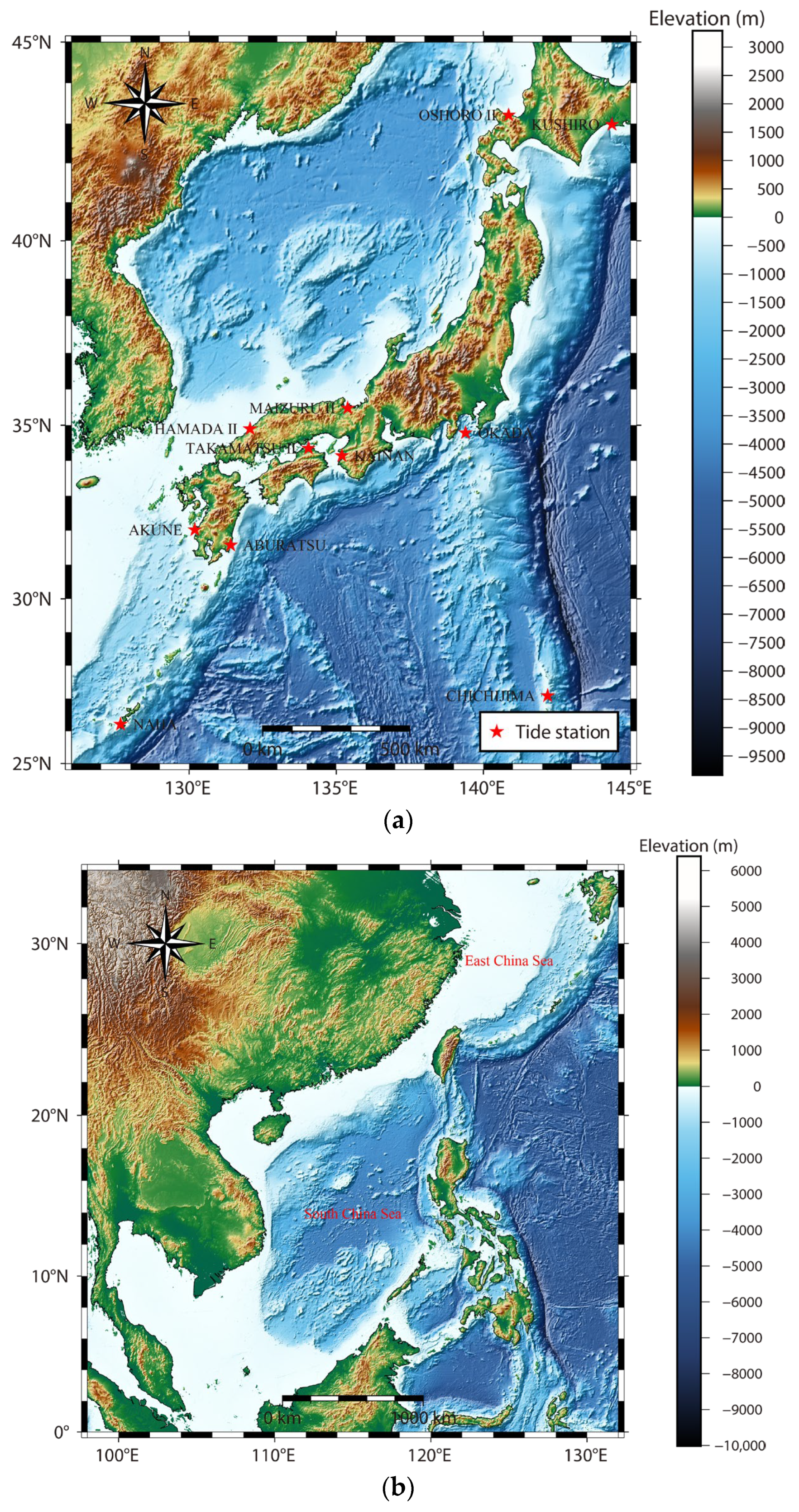
The study region encompasses the coastal regions of Japan and the East and South China Seas, as shown in Figure 1. The dataset includes monthly mean sea level data from eleven tidal stations located along the coast of Japan (Table 1; data obtained from https://psmsl.org/data/obtaining/, accessed on 20 March 2025), as well as satellite altimetry-derived monthly SLA data covering the East China Sea (longitude range: 117°09′ E to 131° E; latitude range: 21°54′ N to 33°11′ N) and the South China Sea (longitude range: 99°E to 122°08′ E; latitude range: 1°12′ N to 23°24′ N). The satellite altimetry-derived SLA data range from January 1993 to December 2024, featuring a spatial resolution of 0.125° × 0.125°, and were obtained from Copernicus Marine Environment Monitoring Service (https://data.marine.copernicus.eu/products, accessed on 12 November 2025). Data processing and analysis were performed on a laptop featuring an Intel(R) Core (TM) i7-7700HQ CPU operating at 2.80 GHz, 16.0 GB of RAM, an NVIDIA GeForce GTX 1050 Ti graphics card, and the Windows 10 operating system. All computations were conducted using MATLAB R2023a.

2.2. CNN-BiGRU

CNN demonstrates competitive performance in handling both image and sequential data compared to traditional neural networks. An essential feature of CNN is its capacity to autonomously extract features from time series via convolution operations executed by filters in the convolutional layer [47].
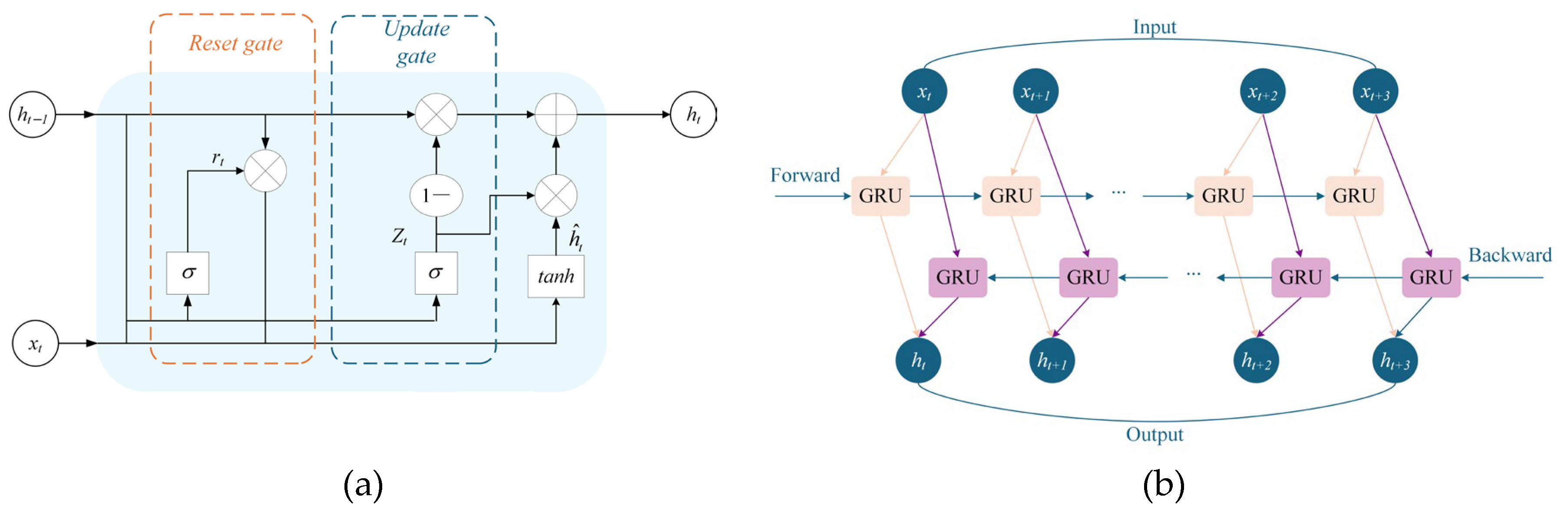
LSTM effectively mitigates the issues of gradient explosion and vanishing gradients encountered when recurrent neural networks (RNNs) process long-term dependencies [48]. The GRU, proposed as an enhancement over LSTM, simplifies the architecture by eliminating the cell state and employing only update and reset gates. This results in a more streamlined structure with fewer parameters while maintaining comparable predictive performance to LSTM. The structural configuration of the GRU model is illustrated in Figure 2a.
Traditional GRU is limited to unidirectional propagation along the sequence, thereby only considering correlations between the current and previous time steps. This approach neglects potentially critical information from future time steps. In scenarios such as sea level height prediction, where past and future data points are likely interrelated, this limitation can significantly impact accuracy. To address this, we introduce a BiGRU network [13], as depicted in Figure 2b.
The BiGRU architecture enhances the traditional GRU by incorporating two GRUs: one processing data in the forward direction according to the time series, and the other in the reverse direction. By fusing outputs from both directions, BiGRU captures comprehensive temporal dependencies, enabling better extraction of global information from the sequence. Consequently, BiGRU provides a richer representation of time series data, leading to improved prediction accuracy.

2.3. Self-Attention Mechanism

Considering the temporal and trend characteristics of monthly mean sea level data, this study uses a variant of the time-specific attention mechanism, namely the SA mechanism [49]. During the training process, the SA mechanism can automatically determine the degree to which different time-step data features contribute to sea level height prediction. It then assigns different weights to different features, reducing the dependence on external information and effectively enhancing the model’s feature extraction capability. Furthermore, the SA mechanism functions by modeling dependencies between sequence elements, thereby integrating global contextual information into each element’s representation. This ability helps in identifying significant trends in sea level variations, which improves the model’s generalization performance on unseen data.
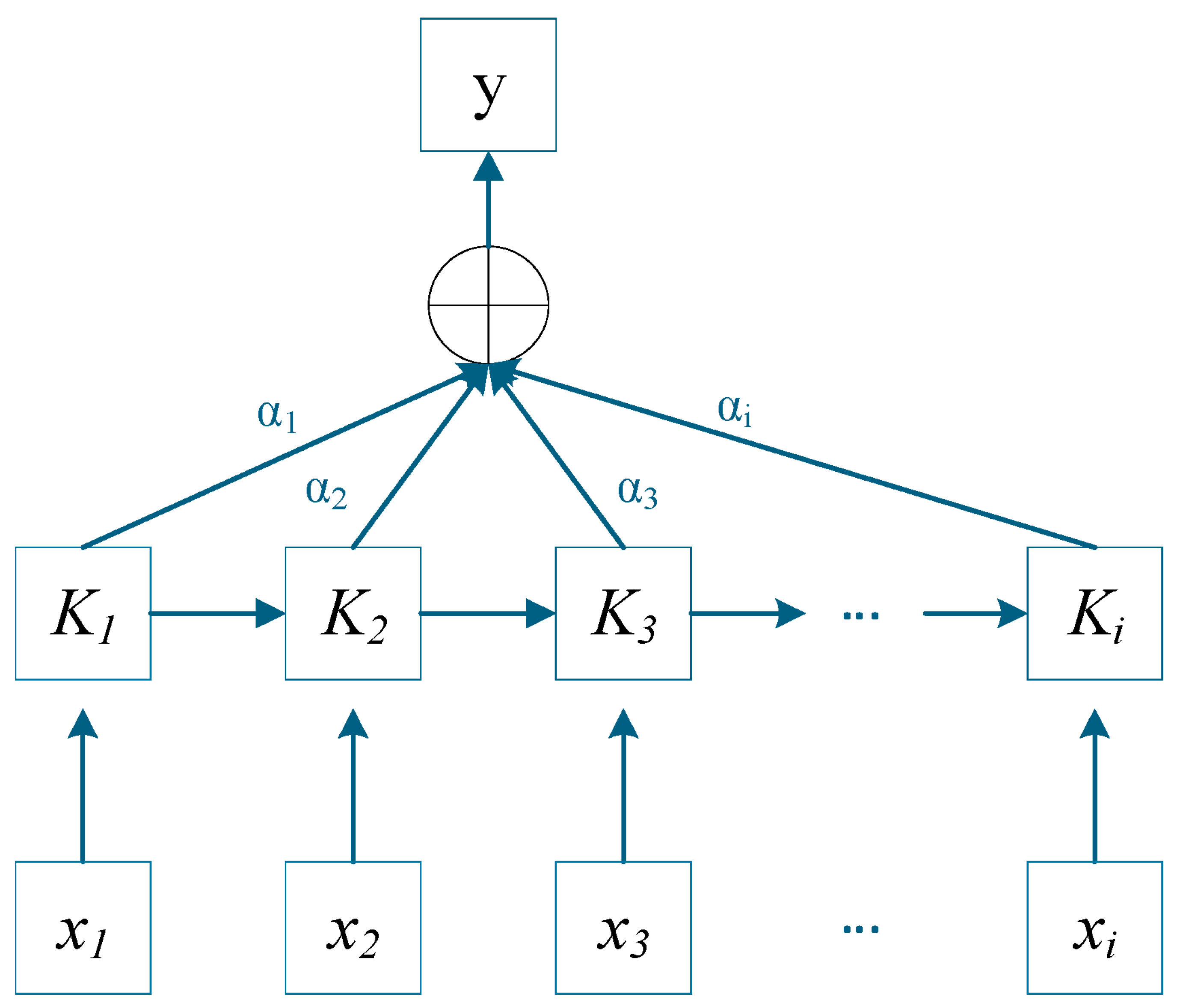
Specifically, the inclusion of the attention mechanism primarily enhances the model’s focus on key information while suppressing irrelevant features. Inspired by the selective attention function of the human brain, this mechanism assigns appropriate weights to hidden state vectors of input sequences at different time steps, thereby highlighting important feature information. This process enables the model to better leverage critical information and ultimately improves prediction accuracy. The structure of the SA mechanism is illustrated in Figure 3. In the figure, x i is the input value; K i is the hidden state outputs from the BiGRU; α i   is the attention weight value; y   is the output data; and i is the data index.
The output sequence from the BiGRU network is passed into an SA module to produce a feature sequence with adaptive weights, as formulated in Equation (1).
A t t e n t i o n Q , K , V = S o f t m a x Q K T d k V
where A t t e n t i o n denotes the resulting attention weights, Q is the query matrix, K is the key matrix, T is the transpose of the matrix, V is the value matrix, d k represents the feature dimension of the keys, and S o f t m a x refers to the normalization function. The SA layer is implemented via the SelfAttentionLayer function from MATLAB’s Deep Learning Toolbox with one attention head and two key/query channels. Through comprehensive experimental validation, this configuration achieves an optimal performance-efficiency balance, particularly suitable for sea-level prediction tasks with limited training data.

2.4. Dream Optimization Algorithm

Reasonable settings of hyperparameters for DL models are essential for model performance evaluation, and intelligent optimization algorithms have strong global search capability and adaptability. Traditional approaches, such as grid search and random sampling, exhibit three critical limitations: (1) computational inefficiency due to exhaustive parameter space exploration; (2) lack of flexibility in adapting to dynamic search spaces; (3) prone to getting trapped in local optima. To address these challenges, Lang and Gao [46] propose the DOA, a novel meta-heuristic approach inspired by human dream cognition mechanisms. Due to space constraints, detailed explanations of the algorithm-related principles are referred to the cited literature [46].
The algorithm mainly consists of an exploration phase and a development phase. In the exploration phase, it guides the search direction through a memory strategy. In the development phase, it prevents falling into a local optimum using a forgetting and supplementation strategy. Additionally, it improves the overall searching ability of the population by combining a dream-sharing strategy. This tripartite architecture emulates key characteristics of human dream processing, including partial memory retention, adaptive forgetting, and logical self-organization, enabling the effective solution of complex optimization problems.
The algorithm strikes an optimal balance between solution space exploration and exploitation through its unique cognitive simulation framework. Quantitative evaluations demonstrate that DOA outperforms traditional optimization methods in three key areas: (1) increased search efficiency via memory-guided pattern recognition; (2) enhanced optimization accuracy via neural self-organization mechanisms; (3) stronger stability through a dynamic balance of forgetting and supplementation. Comparative experiments highlight the proposed algorithm’s significant advantages in convergence speed, solution precision, and stability across benchmark optimization tasks [46].

2.5. The Fusion DOA-CNN-BiGRU- SA Framework

The DL fusion framework introduced in this study consists of four main components: DOA, CNN, BiGRU, and SA. The CNN excels at extracting hidden information from the input sea level change time series through its convolutional operations [34]. The BiGRU effectively establishes long-term dependencies in sequences by utilizing update and reset gates, along with bidirectional processing (forward and backward). Meanwhile, the SA mechanism assists the BiGRU in focusing on the most critical information, thereby enhancing its contribution to the output of the proposed architecture.
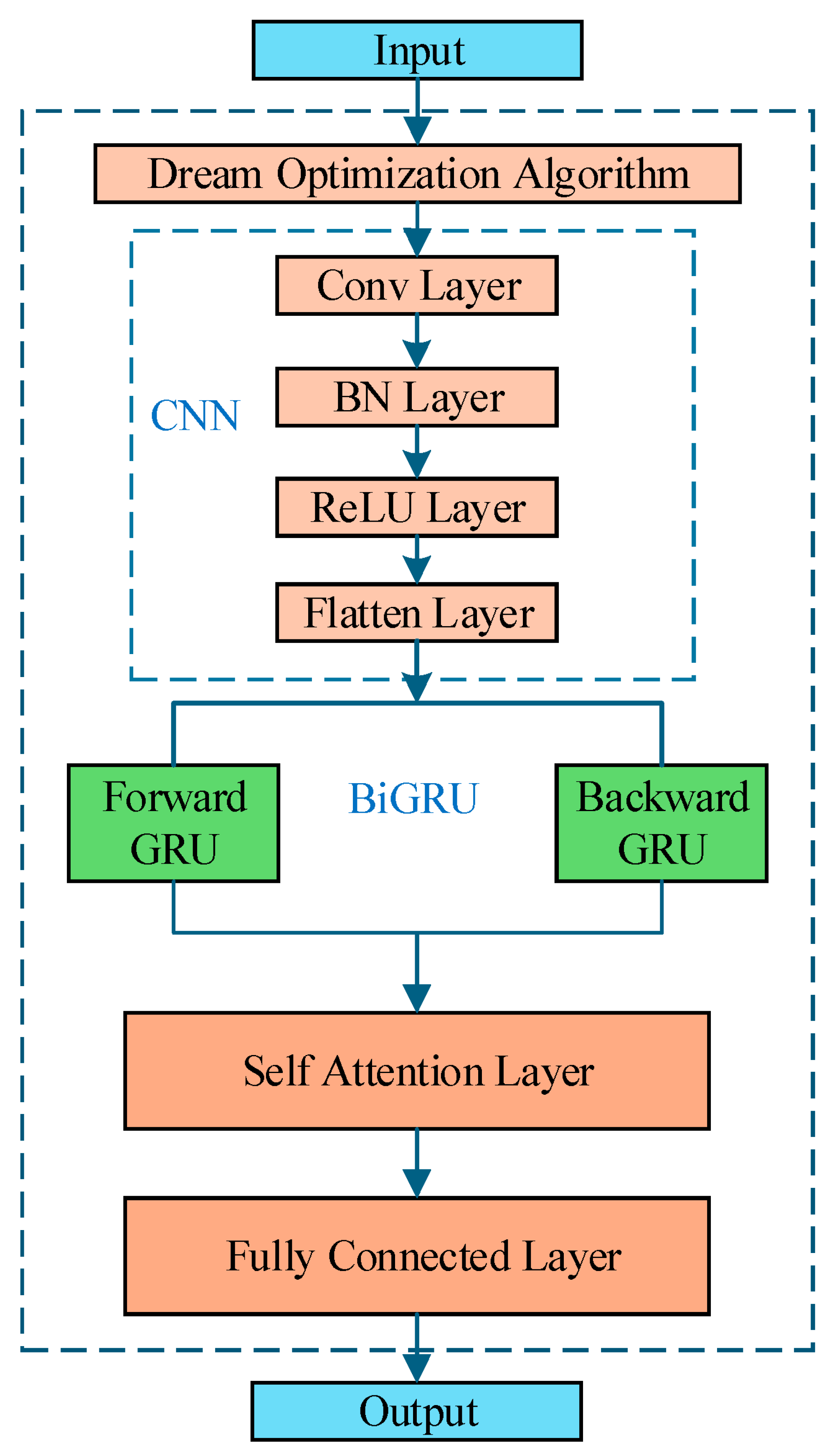
As shown in Figure 4, for the feature matrix constructed from sea level data over time, the DOA is utilized to optimize the hyperparameters of the fusion model (CNN-BiGRU-SA), including the initial learning rate, the number of BiGRU hidden layer units, and regularization parameters. First, during the process of optimizing the hyperparameters of the fusion model, the CNN layer extracts the initial key features from the sequence. Second, the BiGRU is applied to capture long-term temporal dependencies within the data. To further improve predictive accuracy, the SA module dynamically assigns importance weights to different features, emphasizing those most relevant for forecasting while refining earlier feature representations. Finally, a fully connected layer maps multiple important features into one-dimensional space.
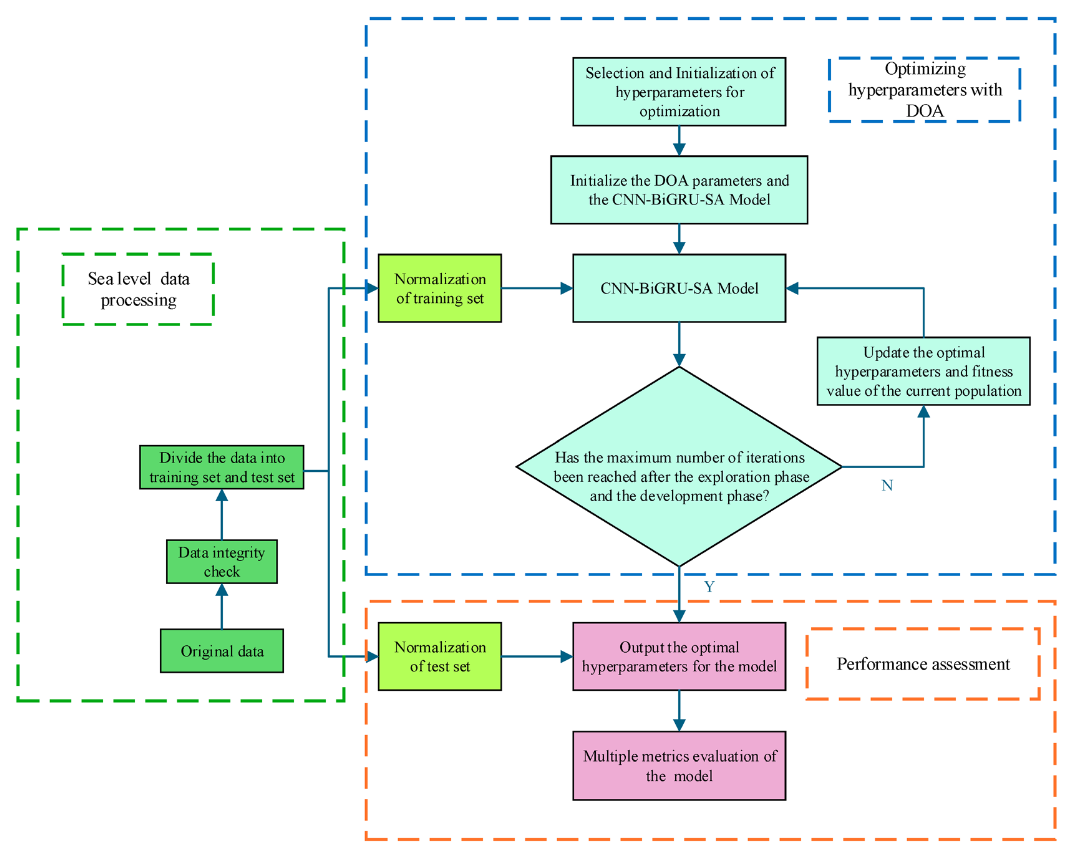
In this architecture, the batch normalization (BN) layer plays a crucial role in accelerating training and convergence while mitigating issues related to vanishing and exploding gradients. The rectified linear unit (ReLU) activation layer introduces nonlinearity, allowing the network to capture increasingly complex patterns in the data. Additionally, the flatten layer reshapes multidimensional tensors into one-dimensional vectors, which serve as inputs to the fully connected layer while preserving the batch dimension. The training and prediction workflow of the proposed model framework is depicted in Figure 5.

2.6. Parameter Setting

This study used a single-step prediction method, employing a sliding window of size 12 as the input data sequence for the model, with an output dimension of 1 corresponding to the predicted value for the next time step. The sea level data were divided into training and test sets in an 8:2 ratio. For all models except DOA-CNN-BiGRU-SA, parameters were optimized iteratively, with a maximum of 200 epochs, an initial learning rate of 0.01, an L2 regularization parameter of 0.001, and the Adam optimizer. To assess the performance of the proposed model, a comparison was conducted against the relevant models listed in Table 2. In the Discussion section, to ensure a fair comparison, the initialization strategies and the number of layers in the existing fusion frameworks (CNN-LSTM, CNN-BiLSTM, and CNN-GRU) were aligned with those of the proposed CNN-BiGRU framework.

2.7. Evaluation Metrics

In this study, four commonly used prediction class evaluation metrics [50,51,52], namely mean absolute error (MAE), mean absolute percentage error (MAPE), root mean square error (RMSE), and coefficient of determination (R2), are used to quantitatively compare and analyze the prediction values of the models. The formulas for each of the evaluation metrics are as follows:
M A E = 1 M i = 1 M y i y i
M A P E = i = 1 M 1 M y i y i y i × 100 %
R M S E = 1 M i = 1 M y i y i 2
R 2 = 1 i = 1 M y i y i 2 i = 1 M y ¯ i y i 2
Here, y i   represents the true value, y i   denotes the predicted value, y ¯ i   is the mean of the true values, and M indicates the number of data points.

3. Results

As shown in Table 1, this section conducts a study using sea level time series data from the five tidal stations (OSHORO II, NAHA, KAINAN, ABURATSU, and OKADA). The single models compared include the CNN, LSTM, BiLSTM, GRU, and BiGRU models, while the fusion models include the CNN-BiGRU, CNN-BiGRU-SA, and DOA-CNN-BiGRU-SA models. To facilitate a more comprehensive comparison of model performance, the robust empirical mode decomposition (REMD) [53] is employed to decompose and reconstruct the tidal station data, removing high-frequency noise components to obtain denoised data.
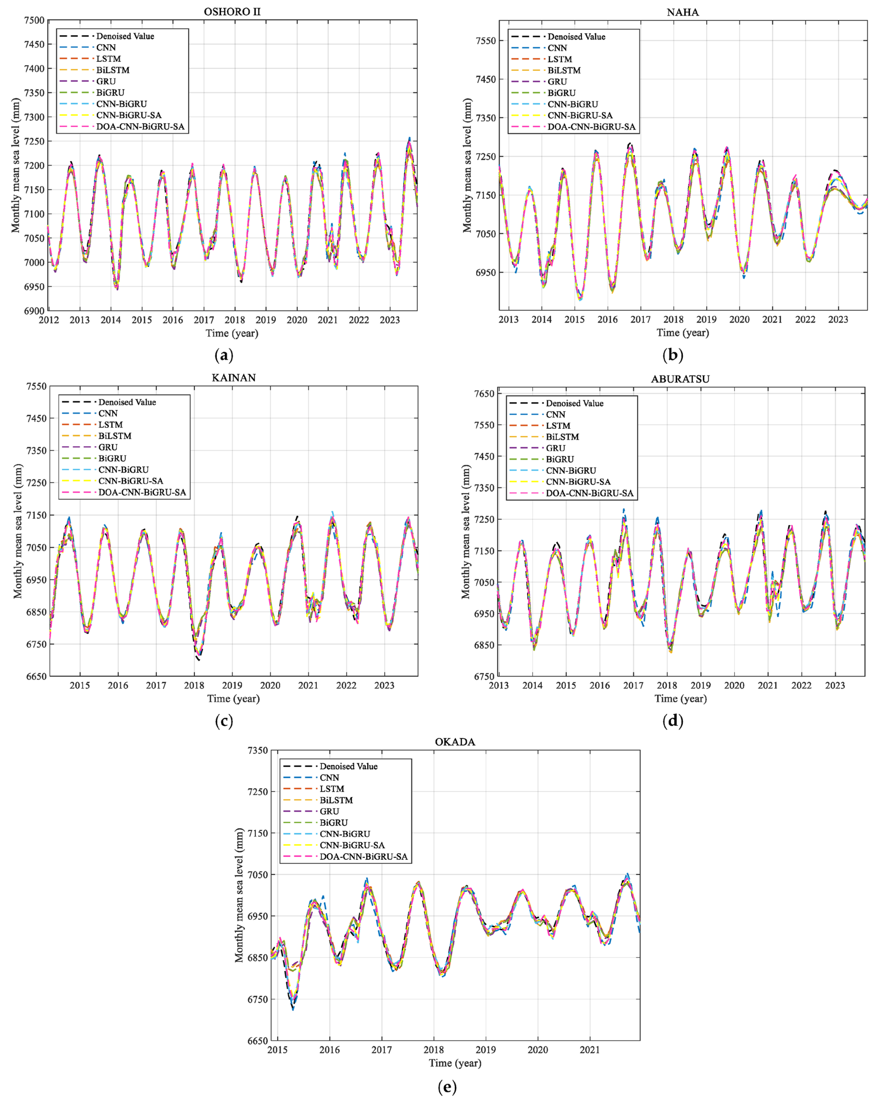
To ensure reproducibility, the random seed for neural network initialization was fixed by resetting it to the default state using MATLAB’s rng(‘default’) function. Figure 6 presents a comparison of test set predictions from eight models across five tidal stations. The results indicate that, while the prediction data from most models align well with the actual data overall, greater deviations in predictions typically occur at points of abrupt change or extreme values. This study highlights the challenge of capturing such detailed variations. Among all models, the DOA-CNN-BiGRU-SA model demonstrates competitive performance, with its predictions exhibiting the closest agreement with the original data.
The specific evaluation metric values for the predictions on the test sets of the five sites are shown in Table 3. Among these tidal stations, the CNN model surpasses other single models (LSTM, BiLSTM, GRU, and BiGRU). Additionally, the BiGRU model outperforms the GRU, LSTM, and BiLSTM models at most tidal stations. By introducing a bidirectional processing mechanism into a unidirectional model, the bidirectional LSTM and bidirectional GRU models are usually able to realize an improvement in performance.
However, the BiGRU model outperforms its unidirectional GRU model across most tidal stations, except for NAHA and KAINAN stations. In contrast, the evaluation metric values of the bidirectional LSTM model are slightly worse than those of the LSTM model, with the exception of the KAINAN station. This distinction may be due to the fact that, for certain sea level data, the LSTM or GRU models may be more appropriate. The bidirectional structure could introduce unnecessary complexity, increasing the risk of overfitting. Additionally, the use of default values for the neural network’s random seed initialization in the DL models may also contribute to performance differences, which can affect the model’s generalization ability. As demonstrated in this experiment, using a default random seed may result in the LSTM and GRU models outperforming their bidirectional counterparts.
The proposed CNN-BiGRU-SA framework, which integrates the strengths of CNN, BiGRU, and SA, demonstrates competitive performance over both the CNN-BiGRU model and other single models. When further optimized using the DOA, the resulting DOA-CNN-BiGRU-SA framework performs better than the seven relevant models in terms of the evaluation metric values. However, incorporating DOA introduces additional computational costs. As the DOA relies on iterative search strategies to identify optimal hyperparameters, the overall training-to-prediction duration for the optimized model increases significantly. Furthermore, the execution time varies across different tidal station datasets, primarily due to differences in sample sizes.

4. Discussion

4.1. Impact of Random Weight Initialization on Model Performance

In the previous chapter, the proposed DOA-CNN-BiGRU-SA framework was assessed using the default random seed for neural network initialization provided in MATLAB R2023a. To ensure the model’s robust generalization capability on unseen data, it is common practice not to fix the random seed during neural network initialization. Consequently, under identical parameter settings, multiple runs on the same data sequence will yield different results due to random initialization. In this section, to enable a fair performance comparison among models under equivalent conditions, a consistent set of random seeds (0, 4, 7, 22, 60, 65, 100, 565, 624, 2025, 3871, 7048, 33658, 44328, 84795, 215432, 437218, 748937, 3284567, 1256321, 4587624, 74326780, 51256781, 85794231, 123456789, 987654321, 578965429, 2334445879, 3587469851, and 4184967296) was used to initialize the weights for training and prediction. Following the prediction process, performance metrics were visualized using boxplots, and statistical analysis was carried out to evaluate the model’s effectiveness. To deepen the evaluation and provide a broader perspective, comparative experiments were conducted against several widely adopted fusion-based models, including the CNN-GRU, CNN-LSTM, and CNN-BiLSTM frameworks.
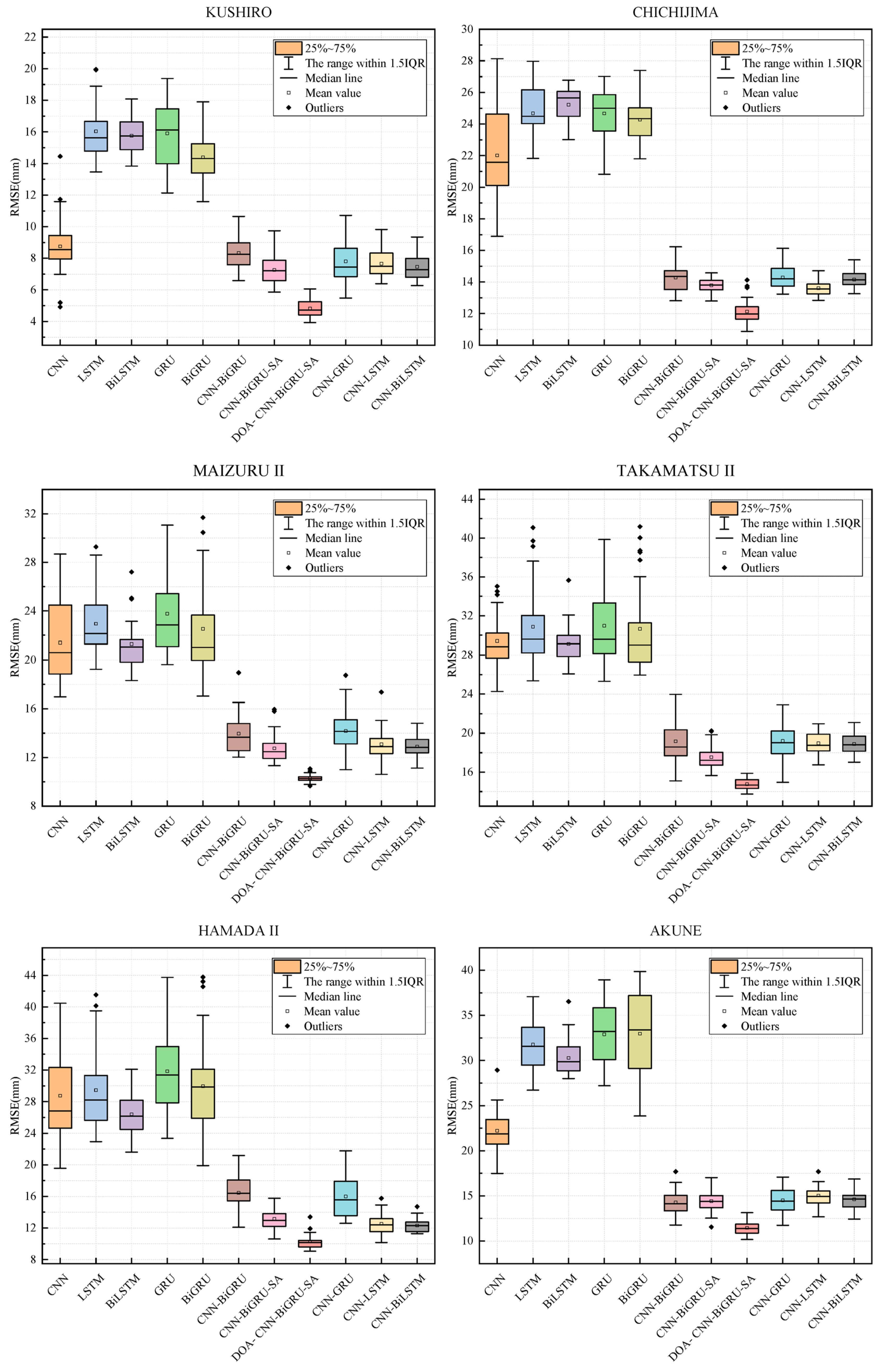
We use the RMSE metric for analysis after 30 random seed trials, as shown in Figure 7. The GRU model exhibits lower maximum RMSE values (or outliers) than the BiGRU model at five stations: CHICHIJIMA, MAIZURU II, TAKAMATSU II, HAMADA II, and AKUNE. In contrast to the GRU model, the BiGRU model achieves lower RMSE values at the KUSHIRO, MAIZURU II, HAMADA II, and AKUNE tidal stations. However, for the BiGRU model, outliers exceeding the maximum RMSE values are observed at MAIZURU II, TAKAMATSU II, and HAMADA II stations, suggesting slightly inferior stability compared to the GRU model. Meanwhile, the BiGRU model exhibits lower RMSE mean and median values across the first five stations, with smaller interquartile ranges (IQRs) in the boxplots, except at the AKUNE station, where its performance is slightly inferior. Based on the detailed analysis, the BiGRU model exhibits better performance than the GRU model across the majority of RMSE metrics.
The BiLSTM model outperforms the LSTM model at all six tidal stations, with lower minimum and maximum RMSE values. The lower mean values of RMSE are achieved by the BiLSTM model at five other stations except the CHICHIJIMA station. Additionally, the BiLSTM model achieves lower median values at MAIZURU II, TAKAMATSU II, HAMADA II, and AKUNE stations. Except for HAMADA II and MAIZURU II stations, the LSTM model obtains the lowest RMSE minimum values at four other stations. However, the LSTM model has a larger IQR than the BiLSTM model, the data of metrics are more dispersed, and outliers exceeding the maximum values are observed at four stations. Overall, both models have their advantages at different stations, but the BiLSTM model is more stable.
Among most of the six tidal stations, the BiGRU model shows lower minimum and median RMSE values compared to the LSTM and BiLSTM models. Specifically, the lowest RMSE minimum values are observed at KUSHIRO, CHICHIJIMA, MAIZURU II, HAMADA II, and AKUNE stations, while the lowest median values are achieved at KUSHIRO, CHICHIJIMA, MAIZURU II, and TAKAMATSU II stations. However, in terms of the mean RMSE, the performance is average, slightly worse than that of the LSTM model or the BiLSTM model at MAIZURU II, TAKAMATSU II, HAMADA II, and AKUNE stations. The constructed CNN model has a large box (IQR) and upper and lower boundary ranges (indicating high inter-data variability), except at CHICHIJIMA, MAIZURU II, and HAMADA II stations.
Across the six tidal stations, the CNN model generally performs better than other single models. Although both the LSTM and GRU models demonstrate certain strengths, the BiGRU model demonstrates slightly reduced robustness. Nonetheless, the BiGRU model typically achieves better performance than both the LSTM and BiLSTM models, a finding that is largely consistent with previous experimental results. Among all fusion models, the integration of the CNN model generally enhances predictive performance compared to single models. Compared to the CNN-BiGRU model, the CNN-BiGRU-SA model exhibits competitive performance, with the lowest RMSE median and mean values at four tidal stations, indicating that the incorporation of an SA mechanism contributes positively to model accuracy.
Compared to the CNN-GRU, CNN-LSTM, and CNN-BiLSTM models, the CNN-BiGRU-SA model shows improved performance with the lowest RMSE median and mean values, and the smallest IQR at most tidal stations. However, it does not achieve the minimum mean at MAIZURU II, TAKAMATSU II, and HAMADA II stations. Additionally, it exhibits higher RMSE maximum values at KUSHIRO, MAIZURU II, TAKAMATSU II, HAMADA II, and AKUNE stations. These results may be attributed to lower data samples or availability at these stations or suboptimal parameter configurations within the SA mechanism, which could constrain the model’s performance.
Compared to the CNN-BiGRU-SA model, hyperparameter optimization via the DOA leads to a notable improvement in predictive accuracy. Additionally, among the compared fusion models, the boxplot for the proposed model exhibits the smallest IQR, indicating a more concentrated data distribution, as shown in Figure 7. Experimental results further validate the high stability of the DOA and highlight the DOA-CNN-BiGRU-SA model’s advantages in both prediction accuracy and robustness.

4.2. Regional Mean Sea Level Change Prediction for the East and South China Seas Region

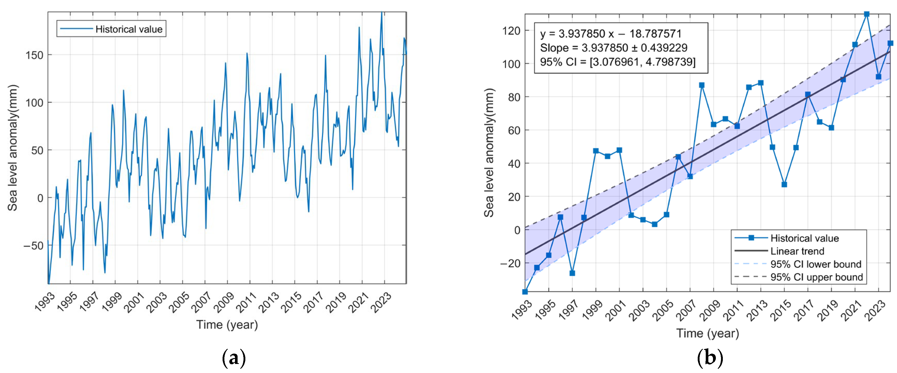
The DOA-CNN-BiGRU-SA model showed competitive predictive performance in a previous comparative study based on tidal station data prediction. To further explore the performance of this model, we use it to predict future satellite altimetry changes in the East and South China Seas region as a whole. As a first step, we process the monthly gridded SLA data for the East and South China Seas using a latitude-longitude area-weighted averaging method, resulting in the average SLA time series data for the region covering 1993–2024 (Figure 8). To better compare with the results of the official bulletin, the data from 1993 to 2022 serve as training data, while the data from 2023 to 2024 serve as test data.
Based on this model, combined with 10 fixed random seeds (0, 22, 624, 7048, 84795, 748937, 3284567, 51256781, 578965429, and 4184967296) for training, the 12 historical(observed) values at the end of the 1993–2022 sequence are selected for rolling prediction, and the predictions obtained from these 10 fixed random seeds are averaged in order to finalize the predictions from 2023 to 2024. To further evaluate the prediction capability of our model, we employ two distinct processing strategies for the 1993–2024 dataset: (1) we first denoise the data using REMD, then train the model on data from 1993 to 2022 to predict 2023–2024; (2) we directly train the model on the raw data from 1993 to 2022 and test it on the raw data from 2023 to 2024.
(1)
The first strategy
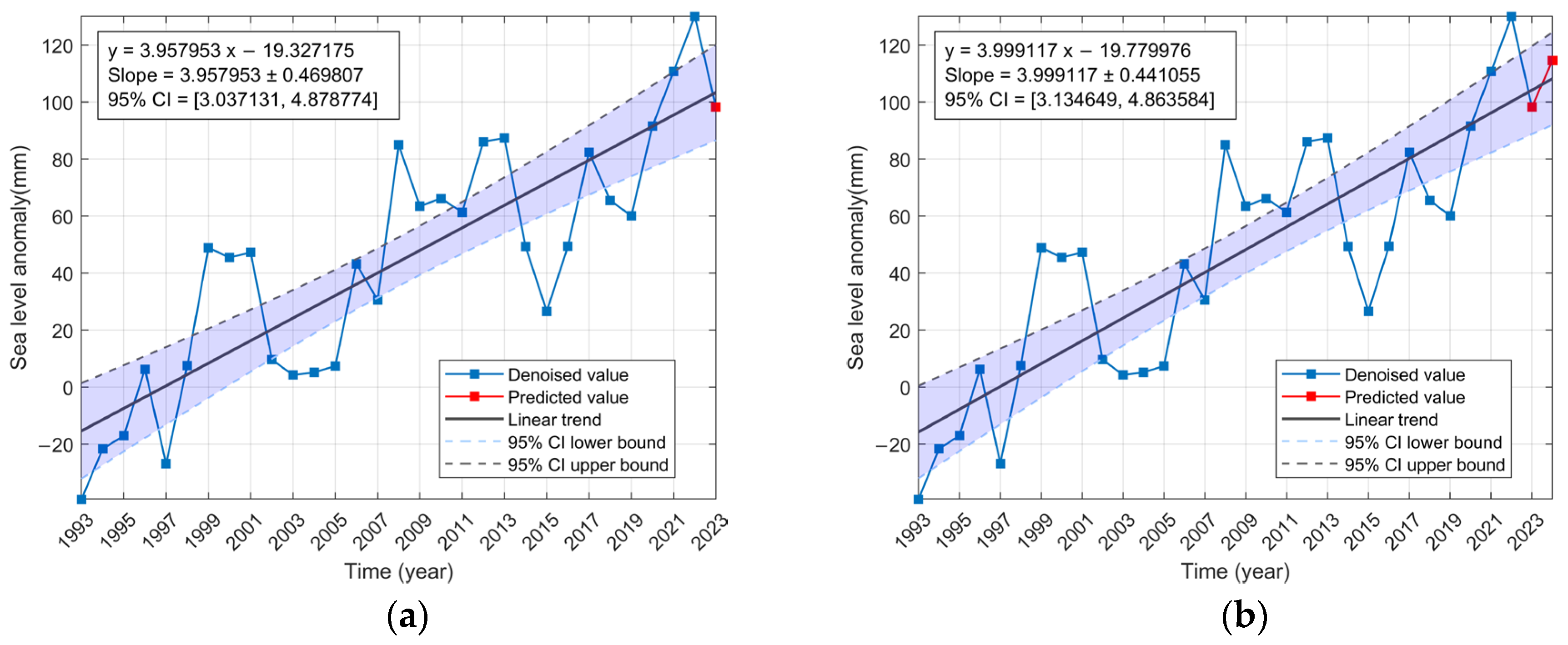
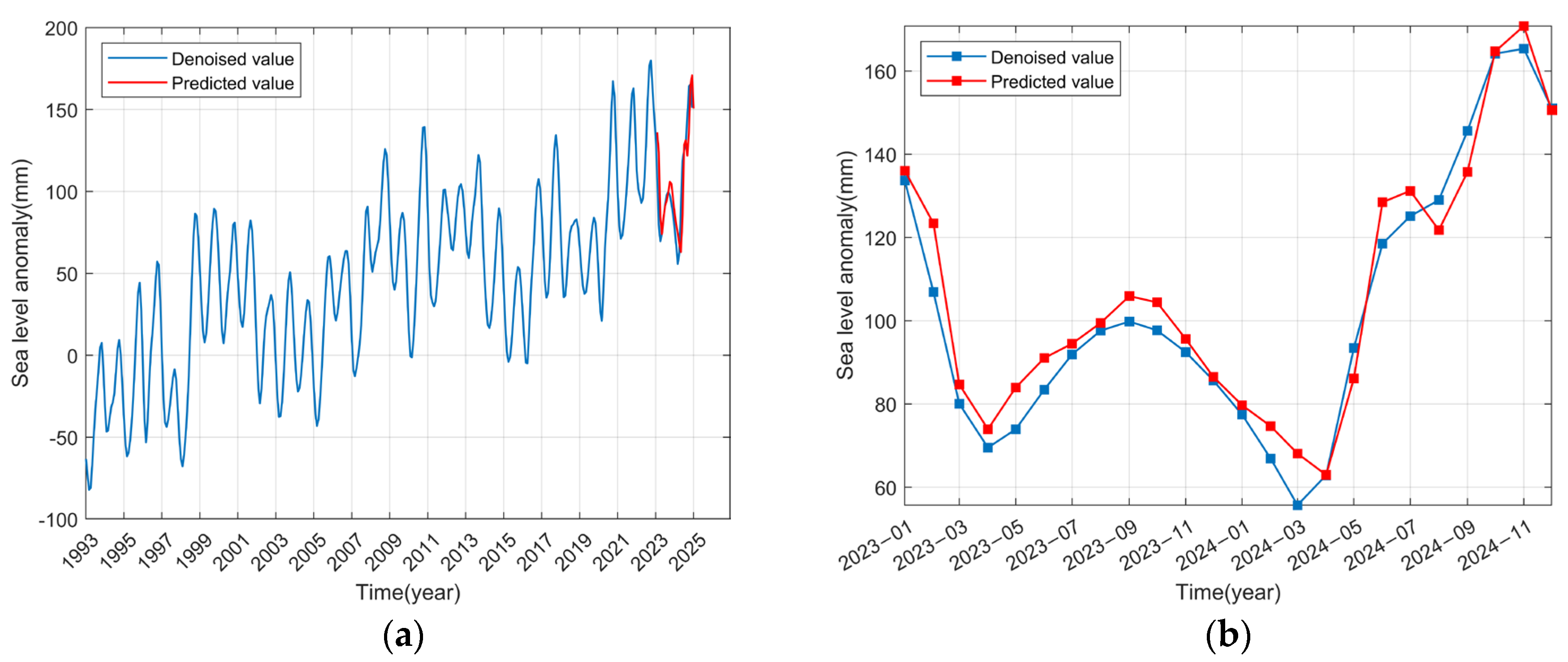
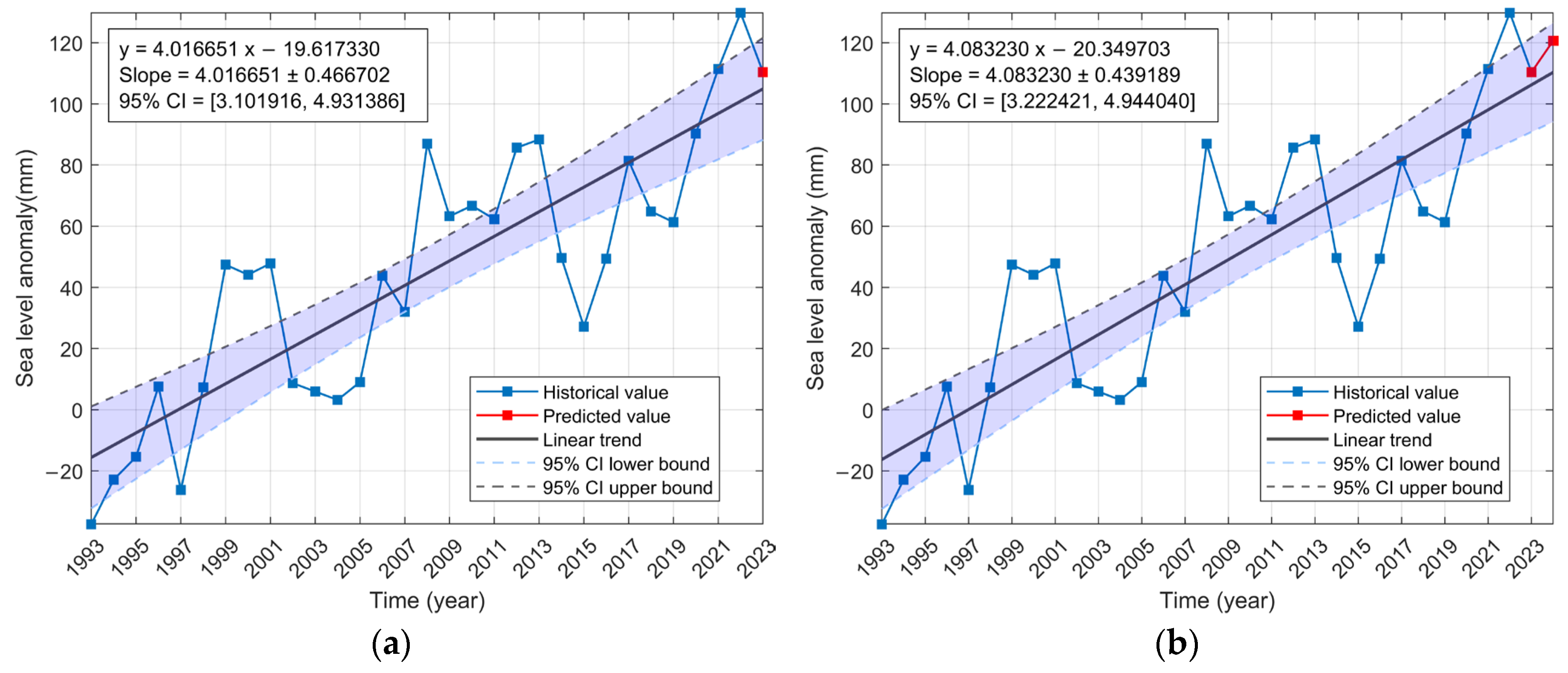
The high-frequency noise is removed from the data via REMD to create the 1993–2022 training set. Figure 9a displays the monthly mean SLA (1993–2024), and its linear trend is estimated using least-squares fitting at a 95% confidence interval (CI). The resulting trend is 3.96 ± 0.47 mm/year, consistent with the rate of sea level rise along China’s coastal areas reported in the official bulletin [54], which documented an increase of 4.00 mm/year from 1993 to 2023. Similarly, the SLA time series in Figure 9a exhibits a linear trend of 4.00 ± 0.44 mm/year (95% CI), which is consistent with both the long-term upward trend observed over the past 31 years (1993–2023) and the rise rate derived from the original observational data in Figure 8b. The prediction results shown in Figure 9b exhibit excellent consistency with the test data, with an RMSE of 6.980 mm, demonstrating the model’s effective forecasting capability. The analysis demonstrates that the proposed method is reliable for SLA forecasting, with prediction errors primarily occurring at abrupt change points and extreme values, validating the effectiveness of this approach for predicting sea level changes. The detailed linear trend and its CI are illustrated in Figure 10, indicating a predicted upward trend in sea level change from 2023 to 2024 in the short term.
(2)
The second strategy
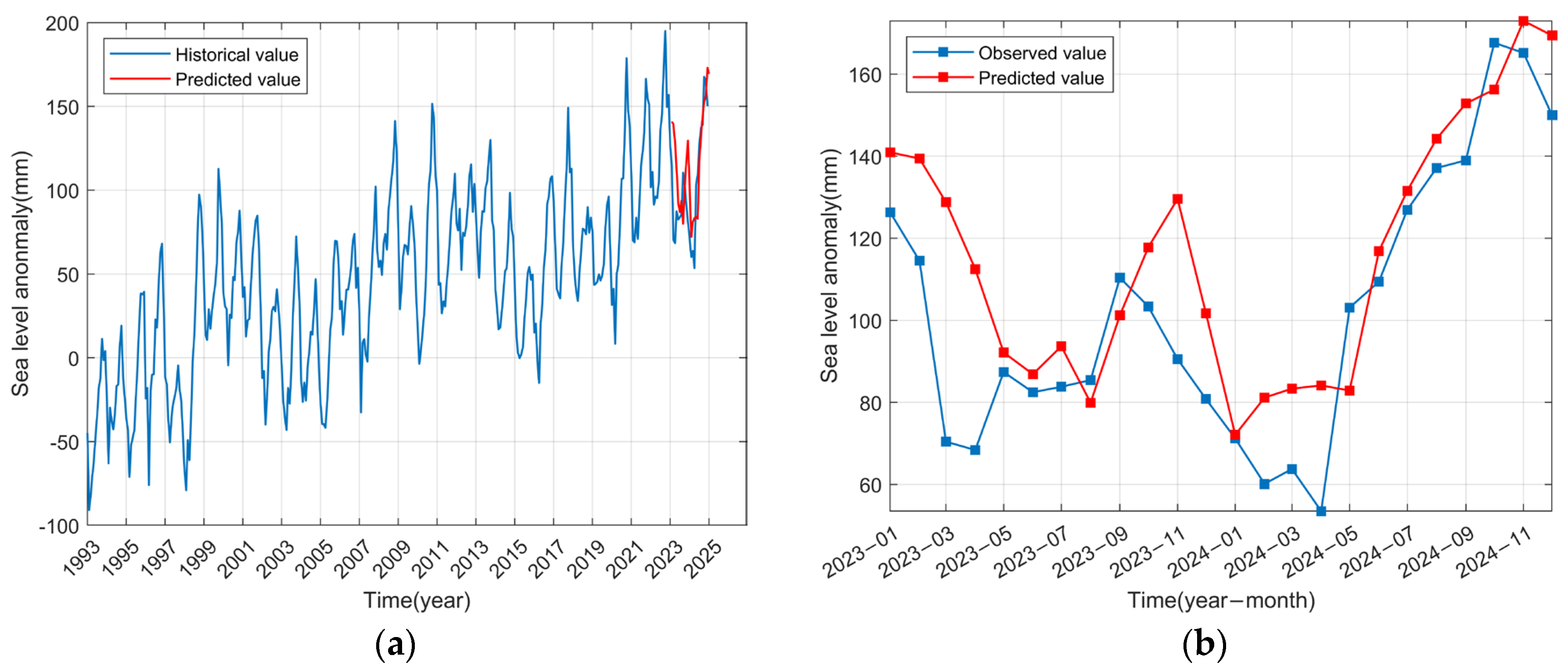
In contrast, this approach utilizes the raw data spanning 1993–2024, partitioning it into a training period (1993–2022) and a forecasting window (2023–2024). The monthly mean SLA shown in Figure 11a yields a least-squares linear trend of 4.02 ± 0.47 mm/year (95% CI) for 1993–2023. This trend, illustrated in Figure 12a, is nearly identical to the 4.00 mm/year coastal rise documented in the China Sea Level Bulletin [54]. An independent trend estimate directly from the full SLA record in Figure 11a is 4.08 ± 0.44 mm/year (95% CI), as shown in Figure 12b, and aligns well with the established 31-year upward trend (1993–2023). However, the corresponding forecasts in Figure 11b have a substantially higher RMSE of 22.035 mm, suggesting heightened sensitivity to high-frequency noise in the input data. Nevertheless, the proposed model retains moderate predictive skill, which is sufficient for operational forecasting in coastal regions, although errors are markedly amplified during periods of rapid change and at extreme values, likely due to unfiltered noise.
(3)
Comparison with the baseline models
For comparison, we assess the two baseline methods (month-wise linear extrapolation and annual-trend-plus-annual-cycle) against the proposed DOA-CNN-BiGRU-SA model. Using the same training and test sets for the combined East and South China Seas, we computed the root mean square errors (RMSE) for both the raw data and the REMD-denoised data over the period 2023–2024. For the month-wise linear extrapolation, the RMSE is 25.287 mm on raw data and 24.068 mm on denoised data; for the annual-trend-plus-annual-cycle method, the RMSE is 52.709 mm on raw data and 51.273 mm on denoised data. In contrast, the DOA-CNN-BiGRU-SA model achieves an RMSE of 6.980 mm under Strategy 1 (REMD-denoised data) and 22.035 mm under Strategy 2 (raw data). Even the best-performing baseline (month-wise linear extrapolation on denoised data, 24.068 mm) produces an error more than three times larger than that of our model under Strategy 1 (6.98 mm). On raw data, our model (22.035 mm) also outperforms the corresponding baseline (25.287 mm). These clear improvements confirm the ability of the proposed framework to capture nonlinear and non-stationary patterns beyond a simple linear trend and annual cycle.
Overall, the combined analysis of both evaluation approaches demonstrates that the proposed framework (DOA-CNN-BiGRU-SA) is reliable for short-term sea level prediction.

4.3. Model Limitations and Impact on Prediction Performance

On monthly to interannual timescales, deviations from the mean annual cycle are largely driven by future atmospheric weather patterns and ocean currents and cannot be predicted from historical sea level time series alone. Therefore, our model is designed to predict total sea level (including the annual cycle and trend), which is of practical value for coastal management. The improvements over other models (Table 3) indicate that the proposed framework captures some nonlinear and non-stationary patterns beyond a simple annual cycle, but we do not claim predictive skill for chaotic weather-driven residuals.
Based on the above research findings, the DOA-CNN-BiGRU-SA model exhibits several limitations that impact its prediction performance. First, the model shows dependence on data availability, as indicated by elevated RMSE values (approximately 12–14 mm) at certain tidal stations (e.g., CHICHIJIMA, HAMADA II). This disadvantage may stem from the fact that the training data at these locations have many mutation points and large fluctuations, which constrain predictive performance, a challenge also noted in sea level forecasting for complex regions like the Baltic Sea [55]. Second, the SA layer is implemented via the selfAttentionLayer function from MATLAB’s Deep Learning Toolbox. The parameter configuration within the SA mechanism may be suboptimal, affecting the model’s prediction accuracy in specific regions and resulting in outliers at certain stations. In contrast, more sophisticated attention implementations, such as the hierarchical stacked spatiotemporal self-attention network, which captures complex oceanic processes, have demonstrated higher efficacy in forecasting sea surface temperatures [39]. Third, the hyperparameters of all baseline models (excluding DOA-CNN-BiGRU-SA) are configured through empirical tuning based on repeated trials and established practices in the literature [56,57,58]. Although not necessarily optimal, this approach yields competitive performance. Additionally, the model shows relatively larger errors at abrupt change points and extreme values, particularly when the data is noisy. This aspect is a common limitation in time series models, indicating that the model’s capacity to capture anomalous sea level variations needs improvement. Including the physical drivers of sea level change as input variables, such as wind speed, surface pressure, and sea surface temperature, could enhance the model’s ability to predict these anomalies, as demonstrated in hydrodynamic-informed deep learning models [29,55]. Finally, the model’s performance varies across different tidal stations, suggesting that the model’s generalization capability may have limitations in different marine regions, necessitating further optimization for specific areas. Similar regional variability has been observed in global assessments of neural network models for surge predictions, which showed much higher performance in mid-latitudes compared to tropical regions [29]. These limitations may affect the model’s short-term predictive accuracy to some degree, but they do not significantly lower its overall accuracy and stability, making it a favorable choice for sea level forecasting.

5. Conclusions

This work proposes a fusion DL framework by integrating the Dream Optimization Algorithm (DOA), a convolutional neural network (CNN), a bidirectional gated recurrent unit (BiGRU), and self-attention (SA). The DOA is applied to optimize the CNN-BiGRU-SA framework, resulting in the DOA-CNN-BiGRU-SA framework. Extensive prediction experiments were performed using monthly sea level data from eleven tidal stations in Japanese waters, where neural network weights were initialized using both default and random seeds. The proposed framework was compared with multiple models and further applied to satellite altimetry data from the East and South China Seas. The following conclusions are drawn.
(1)
Under default seed settings for neural network weight initialization, bidirectional models do not necessarily outperform unidirectional models, and the default seed may constrain the generalization ability. Statistical analysis with multiple random seeds reveals that BiGRU generally outperforms GRU in predictive performance but exhibits lower stability. LSTM and BiLSTM demonstrate variable performance across different stations, with LSTM being less robust. Among the single models, CNN achieves the best overall performance. Fusion frameworks incorporating CNN consistently outperform their counterparts, particularly the CNN-BiGRU-SA model, which demonstrates competitive feature extraction capabilities and enhanced prediction accuracy.
(2)
A well-chosen combination of hyperparameters significantly impacts DL model performance. Optimized with DOA, the CNN-BiGRU-SA model achieves enhanced predictive accuracy and robustness. Based on satellite altimetry data from the combined East and South China Seas, iterative rolling predictions using two distinct strategies yield sea level rise rates of 3.96 ± 0.47 mm/year and 4.02 ± 0.47 mm/year over the period 1993–2023, consistent with the trends reported in the China Sea Level Bulletin (2023) [54]. Predictions for 2023–2024 from both strategies are in good agreement with observations, supporting the potential for short-term sea level forecasting and indicating an upward trend.
(3)
Despite the proposed model’s good performance in predicting sea level changes under small-sample conditions, it still requires improvement. It should be noted that the model is designed to predict total sea level (including the annual cycle and trend) rather than unpredictable weather-driven residuals, which is of practical value for coastal management. Future work may involve developing efficient optimization algorithms to accelerate the hyperparameter search process. Additionally, exploring methods that integrate multiple influencing factors with DL models or climate models, for multi-scale prediction analysis, may yield more stable and precise prediction outcomes.

Author Contributions

Conceptualization, H.W. and F.W.; Methodology, H.W.; Validation, H.W.; Formal analysis, T.L.; Resources, S.Z. and T.L.; Data curation, H.W.; Writing—original draft, H.W.; Writing—review & editing, S.Z. and F.W.; Supervision, S.Z. and T.L.; Funding acquisition, S.Z., T.L. and H.W. All authors have read and agreed to the published version of the manuscript.

Funding

This work was mainly sponsored by the National Natural Science Foundation of China (grant numbers 42374040, 42064001); the Graduate Innovation Fund of East China University of Technology (grant number YC2024-B205).

Data Availability Statement

The monthly mean sea level data were downloaded from the Permanent Service for Mean Sea Level (PSMSL) website (https://www.psmsl.org/). The monthly SLA products, derived from satellite altimetry gridded data and provided by from CMEMS’s website (https://data.marine.copernicus.eu/products, accessed on 12 November 2025).

Conflicts of Interest

The authors declare no conflicts of interest.

References

  1. Hamlington, B.D.; Gardner, A.S.; Ivins, E.; Lenaerts, J.T.M.; Reager, J.T.; Trossman, D.S.; Zaron, E.D.; Adhikari, S.; Arendt, A.; Aschwanden, A.; et al. Understanding of Contemporary Regional Sea-Level Change and the Implications for the Future. Rev. Geophys. 2020, 58, e2019RG000672. [Google Scholar] [CrossRef]
  2. Proshutinsky, A.; Ashik, I.; Dvorkin, E.; Hakkinen, S.; Krishfield, R.; Peltier, W. Secular Sea Level Change in the Russian Sector of the Arctic Ocean. J. Geophys. Res. Ocean. 2004, 109, C03042. [Google Scholar] [CrossRef]
  3. DeConto, R.M.; Pollard, D.; Alley, R.B.; Velicogna, I.; Gasson, E.; Gomez, N.; Sadai, S.; Condron, A.; Gilford, D.M.; Ashe, E.L.; et al. The Paris Climate Agreement and Future Sea-Level Rise from Antarctica. Nature 2021, 593, 83–89. [Google Scholar] [CrossRef] [PubMed]
  4. Bamber, J.L.; Oppenheimer, M.; Kopp, R.E.; Aspinall, W.P.; Cooke, R.M. Ice sheet contributions to future sea-level rise from structured expert judgment. Proc. Natl. Acad. Sci. USA 2019, 116, 11195–11200. [Google Scholar] [CrossRef] [PubMed]
  5. Nicholls, R.J.; Cazenave, A. Sea-Level Rise and Its Impact on Coastal Zones. Science 2010, 328, 1517–1520. [Google Scholar] [CrossRef]
  6. Guillou, N.; Chapalain, G. Machine Learning Methods Applied to Sea Level Predictions in the Upper Part of a Tidal Estuary. Oceanologia 2021, 63, 531–544. [Google Scholar] [CrossRef]
  7. Siqueira, B.V.P.d.; Paiva, A.d.M. Using Neural Network to Improve Sea Level Prediction along the Southeastern Brazilian Coast. Ocean Model. 2021, 168, 101898. [Google Scholar] [CrossRef]
  8. Zhao, J.; Cai, R.; Sun, W. Regional Sea Level Changes Prediction Integrated with Singular Spectrum Analysis and Long-Short-term Memory Network. Adv. Space Res. 2021, 68, 4534–4543. [Google Scholar] [CrossRef]
  9. Xiao, C.; Chen, N.; Hu, C.; Wang, K.; Gong, J.; Chen, Z. Short and Mid-Term Sea Surface Temperature Prediction Using Time-Series Satellite Data and LSTM-AdaBoost Combination Approach. Remote Sens. Environ. 2019, 233, 111358. [Google Scholar] [CrossRef]
  10. Yan, Y.; Xing, H.-Y. A Sea Clutter Detection Method Based on LSTM Error Frequency Domain Conversion. Alex. Eng. J. 2021, 61, 883–891. [Google Scholar] [CrossRef]
  11. Acosta, M.C.; Palomas, S.; Paronuzzi Ticco, S.V.; Utrera, G.; Biercamp, J.; Bretonniere, P.A.; Budich, R.; Castrillo, M.; Caubel, A.; Doblas-Reyes, F.; et al. The computational and energy cost of simulation and storage for climate science: Lessons from CMIP6. Geosci. Model Dev. 2024, 17, 3081–3098. [Google Scholar] [CrossRef]
  12. Zhang, C.; Yang, S.; Huang, X.; Dou, Y.; Li, F.; Xu, X.; Hao, Q.; Gao, J. Sea Level Change and Kuroshio Intrusion Dominated Taiwan Sediment Source-to-sink Processes in the Northeastern South China Sea over the Past 244 Kyrs. Quat. Sci. Rev. 2022, 287, 107558. [Google Scholar] [CrossRef]
  13. Zhang, J.P.; Tomczak, M.; Witkowski, A.; Zhen, X.; Li, C. A fossil diatom-based reconstruction of sea-level changes for the Late Pleistocene and Holocene period in the NW South China Sea. Oceanologia 2023, 65, 211–229. [Google Scholar] [CrossRef]
  14. Yang, S.; Gu, F.; Song, B.; Ye, S.; Yuan, Y.; He, L.; Li, J.; Zhao, G.; Ding, X.; Pei, S.; et al. Holocene Vegetation History and Responses to Climate and Sea-Level Change in the Liaohe Delta, Northeast China. Catena 2022, 217, 106438. [Google Scholar] [CrossRef]
  15. Xie, Y.; Zhou, S.; Wang, F. Prediction Analysis of Sea Level Change in the China Adjacent Seas Based on Singular Spectrum Analysis and Long Short-Term Memory Network. J. Mar. Sci. Eng. 2024, 12, 1397. [Google Scholar] [CrossRef]
  16. Chen, H.; Lu, T.; Huang, J.; He, X.; Sun, X. An Improved VMD–EEMD–LSTM Time Series Hybrid Prediction Model for Sea Surface Height Derived from Satellite Altimetry Data. J. Mar. Sci. Eng. 2023, 11, 2386. [Google Scholar] [CrossRef]
  17. Xiao, M.; Jin, T.; Ding, H. A continuous piecewise polynomial fitting algorithm for trend changing points detection of sea level. Comput. Geosci. 2025, 196, 105876. [Google Scholar] [CrossRef]
  18. Makarynskyy, O.; Makarynska, D.; Kuhn, M.; Featherstone, W. Predicting Sea Level Variations with Artificial Neural Networks at Hillarys Boat Harbour, Western Australia. Estuar. Coast. Shelf Sci. 2004, 61, 351–360. [Google Scholar] [CrossRef]
  19. Alenezi, N.; Alsulaili, A.; Alkhalidi, M. Prediction of Sea Level in the Arabian Gulf Using Artificial Neural Networks. J. Mar. Sci. Eng. 2023, 11, 2052. [Google Scholar] [CrossRef]
  20. Liu, H.M.; He, B.; Qin, P.; Zhang, X.; Guo, S.; Mu, X.K. Sea level anomaly intelligent inversion model based on LSTM-RBF network. Meteorol. Atmos. Phys. 2021, 133, 245–259. [Google Scholar] [CrossRef]
  21. Lou, R.R.; Lv, Z.H.; Dang, S.P.; Su, T.Y.; Li, X.F. Application of machine learning in ocean data. Multimed. Syst. 2023, 29, 1815–1824. [Google Scholar] [CrossRef]
  22. Sun, Q.; Wan, J.; Liu, S. Estimation of Sea Level Variability in the China Sea and Its Vicinity Using the SARIMA and LSTM Models. IEEE J. Sel. Top. Appl. Earth Obs. Remote Sens. 2020, 13, 3317–3326. [Google Scholar] [CrossRef]
  23. Di Nunno, F.; Granata, F.; Gargano, R.; de Marinis, G. Forecasting of Extreme Storm Tide Events Using NARX Neural Network-Based Models. Atmosphere 2021, 12, 512. [Google Scholar] [CrossRef]
  24. Granata, F.; Di Nunno, F. Neuroforecasting of daily streamflows in the UK for short- and medium-term horizons: A novel insight. J. Hydrol. 2023, 624, 129888. [Google Scholar] [CrossRef]
  25. Nunno, F.D.; Marinis, G.d.; Gargano, R.; Granata, F. Tide Prediction in the Venice Lagoon Using Nonlinear Autoregressive Exogenous (NARX) Neural Network. Water 2021, 13, 1173. [Google Scholar] [CrossRef]
  26. Shikhovtsev, A.Y.; Kovadlo, P.G.; Kiselev, A.V.; Eselevich, M.V.; Lukin, V.P. Application of Neural Networks to Estimation and Prediction of Seeing at the Large Solar Telescope Site. Publ. Astron. Soc. Pac. 2023, 135, 014503. [Google Scholar] [CrossRef]
  27. Wu, H.; Zhou, S.; Wang, F.; Lu, T.; Li, X. An optimized network model for sea level height prediction integrating OLSDBO and BiTCN-BiGRU. Dyn. Atmos. Ocean. 2025, 112, 101598. [Google Scholar] [CrossRef]
  28. Raj, N.; Gharineiat, Z.; Ahmed, A.A.M.; Stepanyants, Y. Assessment and Prediction of Sea Level Trend in the South Pacific Region. Remote Sens. 2022, 14, 986. [Google Scholar] [CrossRef]
  29. Tiggeloven, T.; Couasnon, A.; van Straaten, C.; Muis, S.; Ward, P.J. Exploring Deep Learning Capabilities for Surge Predictions in Coastal Areas. Sci. Rep. 2021, 11, 17224. [Google Scholar] [CrossRef]
  30. Fan, S.; Xiao, N.; Dong, S. A Novel Model to Predict Significant Wave Height Based on Long Short-Term Memory Network. Ocean. Eng. 2020, 205, 107298. [Google Scholar] [CrossRef]
  31. Khan, A.R.; Razak, M.S.B.A.; Yusuf, B.B.; Shafri, H.Z.B.M.; Mohamad, N.B. Future Prediction of Coastal Recession Using Convolutional Neural Network. Estuar. Coast. Shelf Sci. 2024, 299, 108667. [Google Scholar] [CrossRef]
  32. Raj, N. Prediction of Sea Level with Vertical Land Movement Correction Using Deep Learning. Mathematics 2022, 10, 4533. [Google Scholar] [CrossRef]
  33. Raj, N.; Murali, J.; Singh-Peterson, L.; Downs, N. Prediction of Sea Level Using Double Data Decomposition and Hybrid Deep Learning Model for Northern Territory, Australia. Mathematics 2024, 12, 2376. [Google Scholar] [CrossRef]
  34. Li, X.; Zhou, S.; Wang, F.; Fu, L. An improved sparrow search algorithm and CNN-BiLSTM neural network for predicting sea level height. Sci. Rep. 2024, 14, 4560. [Google Scholar] [CrossRef] [PubMed]
  35. Nieves, V.; Radin, C.; Camps-Valls, G. Predicting Regional Coastal Sea Level Changes with Machine Learning. Sci. Rep. 2021, 11, 7650. [Google Scholar] [CrossRef]
  36. Ayinde, A.S.; Yu, H.; Wu, K. Sea Level Variability and Modeling in the Gulf of Guinea Using Supervised Machine Learning. Sci. Rep. 2023, 13, 21318. [Google Scholar] [CrossRef] [PubMed]
  37. Zrira, N.; Kamal-Idrissi, A.; Farssi, R.; Khan, H.A. Time Series Prediction of Sea Surface Temperature Based on BiLSTM Model with Attention Mechanism. J. Sea Res. 2024, 198, 102472. [Google Scholar] [CrossRef]
  38. Bai, Z.; Sun, Z.; Fan, B.; Liu, A.-A.; Wei, Z.; Yin, B. Multiscale Spatio-Temporal Attention Network for Sea Surface Temperature Prediction. IEEE J. Sel. Top. Appl. Earth Obs. Remote Sens. 2025, 18, 5866–5877. [Google Scholar] [CrossRef]
  39. Zhao, Y.; Yang, D.; He, J.; Zhu, K.; Deng, X. Hierarchical Stacked Spatiotemporal Self-Attention Network for Sea Surface Temperature Forecasting. Ocean. Model. 2024, 191, 102427. [Google Scholar] [CrossRef]
  40. Li, G.; Zhang, H.; Lyu, T.; Zhang, H. Regional Significant Wave Height Forecast in the East China Sea Based on the Self-Attention ConvLSTM with SWAN Model. Ocean. Eng. 2024, 312, 119064. [Google Scholar] [CrossRef]
  41. Wang, L.; Wang, X.; Dong, C.; Sun, Y. Wave Predictor Models for Medium and Long Term Based on Dual Attention-Enhanced Transformer. Ocean. Eng. 2024, 310, 118761. [Google Scholar] [CrossRef]
  42. Liu, J.; Jin, B.; Wang, L.; Xu, L. Sea Surface Height Prediction with Deep Learning Based on Attention Mechanism. IEEE Geosci. Remote Sens. Lett. 2022, 19, 1–5. [Google Scholar] [CrossRef]
  43. Katipoğlu, O.M.; Mohammadi, B.; Keblouti, M. Bee-inspired Insights: Unleashing the Potential of Artificial Bee Colony Optimized Hybrid Neural Networks for Enhanced Groundwater Level Time Series Prediction. Environ. Monit. Assess. 2024, 196, 724. [Google Scholar] [CrossRef]
  44. Almaliki, A.H.; Khattak, A. Short- and long-term tidal level forecasting: A novel hybrid TCN LSTM framework. J. Sea Res. 2025, 204. [Google Scholar] [CrossRef]
  45. Fei, K.; Du, H.; Gao, L. Accurate Water Level Predictions in a Tidal Reach: Integration of Physics-based and Machine Learning Approaches. J. Hydrol. 2023, 622, 129705. [Google Scholar] [CrossRef]
  46. Lang, Y.; Gao, Y. Dream Optimization Algorithm (DOA): A Novel Metaheuristic Optimization Algorithm Inspired by Human Dreams and Its Applications to Real-World Engineering Problems. Comput. Methods Appl. Mech. Eng. 2025, 436, 117718. [Google Scholar] [CrossRef]
  47. Li, Z.; Liu, F.; Yang, W.; Peng, S.; Zhou, J. A Survey of Convolutional Neural Networks: Analysis, Applications, and Prospects. IEEE Trans. Neural Netw. Learn. Syst. 2022, 33, 6999–7019. [Google Scholar] [CrossRef] [PubMed]
  48. Zhao, Z.; Yun, S.; Jia, L.; Guo, J.; Meng, Y.; He, N.; Li, X.; Shi, J.; Yang, L. Hybrid VMD-CNN-GRU-based Model for Short-Term Forecasting of Wind Power Considering Spatio-Temporal Features. Eng. Appl. Artif. Intell. 2023, 121, 105982. [Google Scholar] [CrossRef]
  49. Yang, L.; Wang, S.; Chen, X.; Chen, W.; Saad, O.M.; Zhou, X.; Pham, N.; Geng, Z.; Fomel, S.; Chen, Y. High-Fidelity Permeability and Porosity Prediction Using Deep Learning with the Self-Attention Mechanism. IEEE Trans. Neural Netw. Learn. Syst. 2023, 34, 3429–3443. [Google Scholar] [CrossRef] [PubMed]
  50. Elbisy, M.S.; Aljahdali, A.H.; Natto, A.H.; Bakhsh, A.A.; Almaliki, A.F.; Alharthi, M.A.; Hassan, A.O. PREDICTION OF DAILY TIDAL LEVELS ALONG THE CENTRAL COAST OF EASTERN RED SEA USING ARTIFICIAL NEURAL NETWORKS. Int. J. GEOMATE 2020, 19, 54–61. [Google Scholar] [CrossRef]
  51. Yang, C.-H.; Wu, C.-H.; Hsieh, C.-M. Long Short-Term Memory Recurrent Neural Network for Tidal Level Forecasting. ISSS J. Micro Smart Syst. 2020, 8, 159389–159401. [Google Scholar] [CrossRef]
  52. Zaki, I.R.; Annuar, A.Z. Tidal Level Short-Term Prediction Using Back-Propagating Artificial Neural Network (BP-ANN). J. Adv. Res. Appl. Sci. Eng. Technol. 2024, 54, 1–15. [Google Scholar] [CrossRef]
  53. Liu, Z.; Peng, D.; Zuo, M.J.; Xia, J.; Qin, Y. Improved Hilbert–Huang Transform with Soft Sifting Stopping Criterion and Its Application to Fault Diagnosis of Wheelset Bearings. ISA Trans. 2022, 125, 426–444. [Google Scholar] [CrossRef]
  54. Ministry of Natural Resources of the People’s Republic of China. China Sea Level Bulletin 2023. 2024. Available online: https://www.nmdis.org.cn/hygb/zghpmgb/2023nzghpmgb/ (accessed on 1 June 2025).
  55. Rajabi-Kiasari, S.; Ellmann, A.; Delpeche-Ellmann, N. Sea level forecasting using deep recurrent neural networks with high-resolution hydrodynamic model. Appl. Ocean Res. 2025, 157, 104496. [Google Scholar] [CrossRef]
  56. Niu, D.; Yu, M.; Sun, L.; Gao, T.; Wang, K. Short-term Multi-Energy Load Forecasting for Integrated Energy Systems Based on CNN-BiGRU Optimized by Attention Mechanism. Appl. Energy 2022, 313, 118801. [Google Scholar] [CrossRef]
  57. Zhang, D.; Chen, B.; Zhu, H.; Goh, H.H.; Dong, Y.; Wu, T. Short-term wind power prediction based on two-layer decomposition and BiTCN-BiLSTM-attention model. Energy 2023, 285, 128762. [Google Scholar] [CrossRef]
  58. Zhou, Y.; He, X.; Montillet, J.-P.; Wang, S.; Hu, S.; Sun, X.; Huang, J.; Ma, X. An improved ICEEMDAN-MPA-GRU model for GNSS height time series prediction with weighted quality evaluation index. GPS Solut. 2025, 29, 113. [Google Scholar] [CrossRef]
Figure 1. Study region. (a) Tidal stations along the coast of Japan, (b) East China Sea and South China Sea regions.
Jmse 14 00982 g001
Figure 2. Flowchart of the BiGRU architecture. (a) The structure of GRU; (b) the structure of BiGRU.
Jmse 14 00982 g002
Figure 3. Structure of the self-attention mechanism.
Jmse 14 00982 g003
Figure 4. Structure of the DOA-CNN-BiGRU-SA model.
Jmse 14 00982 g004
Figure 5. Prediction flow chart of the DOA-CNN-BiGRU-SA model.
Jmse 14 00982 g005
Figure 6. Comparison of predicted and denoised monthly mean sea level values of different models on the test set of the five tide stations: (a) OSHORO II; (b) NAHA; (c) KAINAN; (d) ABURATSU; (e) OKADA. Note that both the predicted and denoised values are derived from REMD-denoised data to remove high-frequency noise.
Jmse 14 00982 g006
Figure 7. Box plot comparison of different models based on 30 random seed trials using six tidal stations. The box plots show the mean, median, interquartile range, and outliers of RMSE, illustrating the robustness and predictive performance of each model.
Jmse 14 00982 g007
Figure 8. Monthly sea level anomaly (SLA) time series based on satellite altimetry for the combined East and South China Seas from January 1993 to December 2024. (a) The monthly historical value (1993–2024); (b) annual average linear trend with 95% confidence interval (CI) for 1993–2024.
Jmse 14 00982 g008
Figure 9. Denoised and predicted values from the DOA-CNN-BiGRU-SA model (strategy 1, REMD-denoised). (a) Denoised and predicted values from 1993 to 2024; (b) predicted vs. denoised SLA for 2023–2024.
Jmse 14 00982 g009
Figure 10. Annual mean sea level anomaly linear trend and 95% CI in the combined South and East China Seas (the first strategy, REMD-denoised). (a) Trend for the period 1993–2023 (3.96 ± 0.47 mm/year); (b) trend for the period 1993–2024 (4.00 ± 0.44 mm/year). The linear trends are derived from least-squares fitting.
Jmse 14 00982 g010
Figure 11. Observed and predicted values from the DOA-CNN-BiGRU-SA model (the second strategy, raw data). (a) Observed and predicted values from 1993 to 2024; (b) predicted vs. observed SLA for 2023–2024.
Jmse 14 00982 g011
Figure 12. Annual mean sea level anomaly linear trend and 95% CI in the combined South and East China Seas (the second strategy, raw data). (a) Trend for the period 1993–2023 (4.02 ± 0.47 mm/year); (b) trend for the period 1993–2024 (4.08 ± 0.44 mm/year). The linear trends are derived from least-squares fitting.
Jmse 14 00982 g012
Table 1. Information on each tidal station.
StationIDCountryLatitude (N)Longitude (E)Duration (Years)
OSHORO II1027Japan43.209444140.8580561963–2023
NAHA1151Japan26.213333127.6652781966–2023
KAINAN701Japan34.144167135.1913891974–2023
ABURATSU814Japan31.576944131.4094441968–2023
OKADA1091Japan34.789444139.3913891985–2021
KUSHIRO518Japan42.975556144.3713891983–2023
CHICHIJIMA1391Japan27.083333142.1833331980–2023
MAIZURU II1387Japan35.476667135.3869441990–2023
TAKAMATSU II1789Japan34.351389134.0569441992–2023
HAMADA II1585Japan34.897222132.0661111987–2023
AKUNE1265Japan32.017500130.1908331996–2023
Table 2. Parameter settings for comparative models.
ModelsParametersValue
CNNConvolution kernel size3 × 1
LSTMNumber of units in the hidden layer10
BiLSTMNumber of units in LSTM hidden layer 110
Number of units in LSTM hidden layer 210
GRUNumber of units in the hidden layer10
BiGRUNumber of units in GRU hidden layer 110
Number of units in GRU hidden layer 210
CNN-BiGRUConvolution kernel size3 × 1
Number of units in GRU hidden layer 110
Number of units in GRU hidden layer 210
CNN-BiGRU-SAConvolution kernel size3 × 1
Number of units in GRU hidden layer 110
Number of units in GRU hidden layer 210
DOA- CNN-BiGRU-SAPopulation30
Number of iterations10
Initial learning rate0.0001–0.01
Number of units in the BiGRU hidden layer1–100
L2 regularization parameter0.0001–0.01
Table 3. Evaluation metrics for monthly mean sea level predictions by eight models on the REMD-denoised test set of five tidal stations.
StationModelsMAE (mm)MAPE (%)RMSE (mm)R2
OSHORO IICNN8.8730.12512.3970.974
LSTM11.9910.16916.1620.956
BiLSTM12.2420.17216.3130.955
GRU12.7760.18016.8340.952
BiGRU11.2320.15815.0920.962
CNN-BiGRU8.0440.11310.9890.980
CNN-BiGRU-SA7.6680.10810.4660.981
DOA- CNN-BiGRU-SA6.8150.0969.3980.985
NAHACNN10.5190.14813.7990.980
LSTM15.9560.22320.5810.956
BiLSTM16.7020.23420.8010.955
GRU14.3420.20118.0090.966
BiGRU15.1750.21319.2870.961
CNN-BiGRU7.9010.11110.3320.989
CNN-BiGRU-SA6.7530.0959.2490.991
DOA- CNN-BiGRU-SA4.9970.0706.7150.995
KAINANCNN15.0530.21618.8930.971
LSTM19.3880.28027.0490.941
BiLSTM19.0440.27526.5440.943
GRU20.4350.29427.1520.940
BiGRU19.6110.28327.0690.940
CNN-BiGRU11.9940.17315.5400.980
CNN-BiGRU-SA11.0650.15915.0920.981
DOA- CNN-BiGRU-SA9.8660.14213.1780.986
ABURATSUCNN17.3450.24622.6720.956
LSTM21.1200.29827.6810.935
BiLSTM21.2900.30128.3420.932
GRU21.5480.30428.1660.933
BiGRU20.0150.28327.02800.938
CNN-BiGRU13.3310.18817.6270.974
CNN-BiGRU-SA13.0130.18317.4090.974
DOA- CNN-BiGRU-SA10.3050.14613.9550.983
OKADACNN12.2310.17715.4640.948
LSTM14.8950.21622.2730.891
BiLSTM15.3860.22323.1290.883
GRU15.9440.23124.1800.872
BiGRU14.8190.21521.9330.895
CNN-BiGRU9.5200.13812.2140.967
CNN-BiGRU-SA9.0360.13111.8300.969
DOA- CNN-BiGRU-SA8.7980.12710.9580.974
Disclaimer/Publisher’s Note: The statements, opinions and data contained in all publications are solely those of the individual author(s) and contributor(s) and not of MDPI and/or the editor(s). MDPI and/or the editor(s) disclaim responsibility for any injury to people or property resulting from any ideas, methods, instructions or products referred to in the content.