Article

Data Fusion Framework for a High-Resolution Regional Dataset in the Western North Pacific

1
College of Oceanography and Ecological Science, Shanghai Ocean University, Shanghai 201306, China
2
College of Naval Architecture and Ocean Engineering, Naval University of Engineering, Wuhan 430033, China
*
Authors to whom correspondence should be addressed.
J. Mar. Sci. Eng. 2026, 14(11), 976; https://doi.org/10.3390/jmse14110976 (registering DOI)
Submission received: 2 April 2026 / Revised: 23 April 2026 / Accepted: 21 May 2026 / Published: 25 May 2026
(This article belongs to the Special Issue Marine Modelling and Environmental Statistics—2nd Edition)

Abstract

Based on the large volume of observational data obtained from Argo and several satellites, an increasing number of datasets are being developed and applied to oceanographic research. However, there are still problems such as sparse subsurface observations, insufficient parameters, and weak pertinence. This study provides a basic framework for high-resolution data fusion that focuses on the multi-source observations in the Western North Pacific. Multi-source observations from satellites, Argo floats, and historical in situ profiles are fused using a statistical model and a gradient-dependent optimal interpolation method. A daily gridded dataset with a 0.25° horizontal resolution is developed, which includes temperature, salinity, and currents. The results show that the correlation coefficients between the observations and the inverted profiles of temperature and salinity are about 0.99 and 0.94, respectively, with mean root mean square errors of about 1.27 °C and 0.13, respectively. In the Northwest Pacific Ocean, the most suitable parameter settings are a search radius of 1.5° in longitude and latitude, correlation scale constant of 0.25°, and relative observation error of 2. Consequently, the average RMSEs of the fused temperature and salinity fields are 0.43°C and 0.056, respectively. Compared with other reanalysis datasets, the product constructed in this study retains more high-frequency ocean signals, and its temperature error relative to XBT observations is also the smallest. Furthermore, the dataset effectively depicts the characteristics of marine dynamic processes such as the Kuroshio paths and mesoscale eddies.

1. Introduction

Ocean observations are very important for understanding the features and dynamics of the ocean. Prior to the 1990s, oceanographic data were predominantly collected through ship-based measurements. By the late 1990s, the implementation of the World Ocean Circulation Experiment (WOCE) [1] program enabled global scientists to collect ocean data such as temperature, salinity, and dissolved oxygen through ship-based measurements, moored buoys, automatic drifting buoys, and satellite technology. Satellite remote sensing provides round-the-clock monitoring of global ocean surface temperature, salinity, and ocean currents, filling gaps in sea-based observations. The Argo (Array for Real-time Geostrophic Oceanography) observation program, initiated in the early 21st century, enabled real-time monitoring of global ocean subsurface information. At present, the Global Ocean Observing System (GOOS) facilitates international collaborations for collecting relevant ocean observations through multiple methods, including profiling drifters, various forms of moored buoys and platforms, marine high-frequency radar stations, research vessels, volunteer ships, submersible gliders, and animal telemetry [2]. The implementation of these observational programs has amassed vast quantities of observational data for both fundamental and applied oceanographic research. However, due to limitations in their respective observational principles and technical constraints, individual data sources possess inherent limitations and scopes of applicability, and each source can only contain specific oceanic environmental variables within its own temporal and spatial scales. Therefore, using objective analysis methods to fuse multi-source ocean observational data with varying spatial and temporal resolutions can produce datasets that comprehensively reflect diverse marine environmental information and provide essential data support for monitoring ocean dynamics and enhancing climate forecasting and disaster warning capabilities.
With the rapid advancement of satellite observation technology, an increasing number of high-resolution satellite-observed sea surface data products [3] have been used for marine application research. The daily sea surface temperature dataset GHRSST (Group for High Resolution Sea Surface Temperature) was constructed by the Naval Oceanographic Office (NAVO) based on satellite orbital data from instruments such as AVHRR and AMSR, with a spatial resolution of up to 0.1°. The UK Met Office Hadley Centre used the Operational Sea Surface Temperature and Ice Analysis system (OSTIA) to produce a global daily sea surface temperature dataset [4] with a 0.05° spatial resolution based on data from satellites such as AVHRR. The sea surface salinity product [5] from NASA (National Aeronautics and Space Administration), developed based on SMAP satellite observations, featured a spatial resolution of 0.25° and a daily temporal resolution. CMEMS (Copernicus Marine Environment Monitoring Service) and AVISO (Archiving, Validation and Interpretation of Satellite Oceanographic) developed daily gridded datasets [6] with spatial resolutions of 0.25° and 0.125°, based on sea surface height observations from satellites including Sentinel and Jason. Concurrently, a series of scattered datasets observing the interior of the ocean, such as the World Ocean Database (WOD) [7], the Global Temperature and Salinity Profile Programme (GTSPP) [8], and the Argo system, have gradually been established. Furthermore, owing to the spatiotemporal irregularity of raw data, scholars worldwide have developed various ocean gridded datasets using methods including optimal interpolation [9], Kalman filtering [10,11], and variational assimilation [12]. Among these, gridded datasets [13,14,15] derived through objective analysis predominantly feature a monthly temporal resolution and a spatial resolution of 1°, though some datasets [16,17] achieve a spatial resolution of 0.25° with temporal resolutions spanning multi-year monthly averages or multi-year weekly averages. In contrast, reanalysis products derived from numerical models exhibit relatively higher spatiotemporal resolution; for instance, NASA’s ECCO (Estimating the Circulation and Climate of the Ocean) program used the MITgcm circulation model to construct the ECCO-V4r4 dataset with 1° horizontal and daily resolutions [18]. The European Centre for Medium-Range Weather Forecasts (ECMWF) built the Ocean Analysis–Reanalysis System (OCEAN5) based on the NEMO and NEMOVAR models to produce the monthly dataset ORAS5 with a spatial resolution of 0.25°. The GLORYS12V1 (Global Ocean Physics Reanalysis 12V1) dataset produced by CMEMS, based on the NEMO model and the GOFS3.1 product, with a spatial resolution of 1/12° and a daily temporal resolution, offers greater potential for studying small-scale ocean phenomena, along with the Yin-He Global Ocean Data Assimilation and Forecast System [19].
Satellite observations with high spatiotemporal resolution provide comprehensive sea surface data, while Argo profiling buoys and traditional in situ profiling methods complement each other, accumulating massive internal ocean data. The integration of multi-source data through data assimilation and objective analysis methods has become a crucial technical approach for effectively using these valuable data. Data assimilation is commonly employed in numerical models to use observations for reducing model errors, and can be applied to both hindcasts and forecasts. However, compared to objective analysis, data assimilation methods based on numerical models are more complex. Meanwhile, the accuracy of objective analysis depends on the density of observations. In this study, we aim to propose a fusion framework for high-resolution gridded dataset in the northwest Pacific based on observations. First, we use a statistical model [20] to fuse Sea Level Anomaly (SLA), Sea Surface Temperature (SST), Argo data, and other datasets to invert daily profiles, aiming to enhance the density of observational data for reconstruction. Then, based on a gradient-dependent optimal interpolation method, we fuse data from Argo, WOD, and the inverted profiles to reconstruct a daily gridded dataset for the Northwest Pacific Ocean (NWP) (110° E–190° E, 10° N–60° N) in 2023 with a 0.25° horizontal resolution, which includes parameters such as temperature, salinity, and current fields.

2. Materials

2.1. Profiles

The temperature (T) and salinity (S) observational profiles used in this study include Argo data from the China Argo Real-time Data Centre (CARDC) (https://www.argo.org.cn/ accessed, on 21 May 2025) and WOD data from the National Centers for Environmental Information (NCEI). The Argo data were used for profile inversion and dataset reconstruction, and the CTD (conductivity, temperature, and depth) data and the XBT (Expendable Bathythermograph) data from the WOD were used for reconstruction and comparative validation, respectively. A total of 349,679 profiles of temperature and salinity from 1 January 2004 to 31 December 2024 were retained after applying the post-processing quality control procedure developed by CARDC [21,22]. The Amika method was then used to vertically interpolate the quality-controlled profiles into 40 layers spanning 5 to 2000 m (5 m 10:10:100 m 120:20:200 m 250:50:900 m 1000:100:1800 m 2000 m). Over most regions of the NWP, the number of profiles within a 0.25° × 0.25° grid exceeds two, with half of the areas containing more than five profiles (Figure 1a). The number of daily observation profiles in 2023 was more than 60 (Figure 1b).

2.2. Surface Observations

The SLA daily product (Global Ocean Gridded L4 Sea Surface Heights And Derived Variables Reprocessed Copernicus Climate Service) and the multi-year climatology product averaged over 1993–2023 (Global Ocean Mean Sea Level Trend Map from Observations Reprocessing) were derived from the Copernicus Climate Change Service (C3S) with a spatial resolution of 0.25°. The SST multi-year climatology and the daily product with a spatial resolution of 0.25° from the National Oceanic and Atmospheric Administration (NOAA, https://psl.noaa.gov/data/gridded/data.noaa.oisst.v2.highres.html, accessed on 18 June 2025) were used for profile inversion [23]. The SLA daily product originated from the DUACS delayed-time sea-level height anomaly gridded data field, and the sea level ocean monitoring indicators for the climatology product were derived from DUACS delayed sea-level anomalies.

2.3. Subsurface Datasets

The CMEMS weekly dataset (Multi Observation Global Ocean ARMOR3D L4 analysis, Armor-3D) from CLS (Collecte Localisation Satellites) (Toulouse, France), with a spatial resolution of 0.25° and 50 levels in the upper 5500 m, was produced by fusing satellite and observational data. It served as the initial background field for reconstruction [24]. Additionally, multi-year and monthly climatology data from the World Ocean Atlas (WOA), with a spatial resolution of 0.25°, were used to calculate the gradient-dependent correlation scale and served as the initial background field for profile inversion, respectively.
The daily product with a spatial resolution of 0.25° and 75 levels in the upper 5900 m (Global Ocean Ensemble Physics Reanalysis) from CMEMS was used for comparative validation. It contains two datasets: the GLORYS2V4 (Global Ocean Physics Reanalysis 2V4) dataset from Mercator Ocean and the C-GLORSv7 (The CMCC Global Ocean Physical Reanalysis System v7) dataset from CMCC (Euro-Mediterranean Center on Climate Change). Based on the ocean numerical model NEMO with a 0.25° grid resolution (ORCA025), these two datasets were derived through the assimilation of satellite and in situ observations into ocean numerical models using the SAM2 (SEEK) and OceanVar (3DVar) methods, respectively.

3. Methods

3.1. Inversion of T/S Profiles

The statistical model of Guinehut et al. [20], with easy operability and stable results, was used for inversion of the T/S profiles. The synthetic T profiles were derived from altimeter and SST observations, and the S profiles were derived from altimeter observations using a linear regression method, expressed as follows:
T x , y , z , t = α x , y , z , t · S L A T x , y , t + β x , y , z , t · S S T x , y , t + T ¯ x , y , z , t
S x , y , z , t = γ x , y , z , t · S L A S x , y , t + S ¯ x , y , z , t
where SLA′ and SST′ denote anomalies from their respective multi-year climatology; T ¯ and S ¯ denote the WOA monthly climatology; and α, β, and γ are the regression coefficients of the SLAT and SST with respect to temperature and of the SLAS with respect to salinity, respectively. The SLAT and SLAS at the same time and location are identical. The regression coefficients vary with depth, time, and geographical location and are expressed as covariances between the variables (only the z variable is given here for clarity) as follows:
α z = S S T , S S T · S L A T , T z S L A T , S S T · S S T , T z S L A T , S L A T · S S T , S S T S L A T , S S T 2
β z = S L A T , S L A T · S S T , T z S L A T , S S T · S L A T , T z S L A T , S L A T · S S T , S S T S L A T , S S T 2
γ z = S z , S L A S S L A S , S L A S
A , B = 1 n i = 1 n a i A ¯ b i B ¯   ,   i = 1 , , n
where a and b are the observations of variables A and B, respectively. These covariances were calculated using the Argo observations to describe the relationship that exists for each profile between its surface and subsurface properties. T′(z) and S′(z) denote anomalies from the WOA multi-year climatology.

3.2. Gradient-Dependent Optimal Interpolation

Gradient-dependent optimal interpolation is an analysis method based on the optimal interpolation and least-squares theory. The results at the gridded point used for analysis are taken as the background value plus the observational increments weighted by optimal weights. The equation of the influence of M observations on the analysis point is given in Equation (7). An important part of the scheme involves estimating the optimal weights. According to minimum variance theory, the optimal weight can be determined by solving Equation (8) [25].
v i a = v i b + j M ω i j δ y j 0
j = 1 M ω i j μ j k + η k ω i k = μ i k , k = 1 , , M
where v i a is the analysis value and v can be any environmental variable, such as temperature, salinity, or sound velocity. The symbol v i b , given by the background, is the first estimated value. The subscript i denotes the number of gridded points used for analysis, and j and k denote the number of available sites of profiles. The ω i j denotes the optimal weight between gridded point i and observational point j. For observational increments, δ y j 0 = y j 0 H v j b , the observational operator H is used to convert the background into the first guess of the observation y j 0 . Each increment has an optimal weight ω i k associated with the background error correlations μ j k and μ i k . μ j k and μ i k are correlations between the background errors at the two observational points, j and k, and at the analysis and observation points i and k, respectively. The parameter η k is the square of the relative observational errors compared with the background errors. It is frequently set to be a constant η for a single source of observation and “tuned” to vary the weights of the observations.
The correlations are usually assumed to follow a Gaussian exponential function and are inversely proportional to distance [26,27,28], as shown in Equations (9) and (10):
μ i k   ~   e x p x i x k 2 L ϕ / G x 2 y i y k 2 L ϕ / G y 2
G x = 1 + v / x E v / x , G y = 1 + v / y E v / y
where x and y are the longitude and latitude, respectively. The parameter L ϕ is the scale of correlation, which can be obtained from the product of the scale parameter and the cosine function of the latitude ϕ at the analysis gridded point. L ϕ / G depends on the Rossby radius of deformation and changes in the horizontal gradient that define the scale of correlation of the background error. The parameter G, calculated using WOA climatological data, is associated with the horizontal gradient at location i. It contains a zonal component G x and a meridional component G y .

3.3. Calculation of Derived Factors

The geostrophic currents were calculated based on the geostrophic balance from the dynamic height data derived from temperature and salinity [29]. The Kuroshio paths were identified by tracking the locally strongest components within the sea surface current field based on a previously proposed method [30]. Another method [31] was used to identify mesoscale eddies, which represents an automated detection and tracking technique for ocean eddies that defines eddies based on the geometric characteristics of the flow field.

4. Procedure

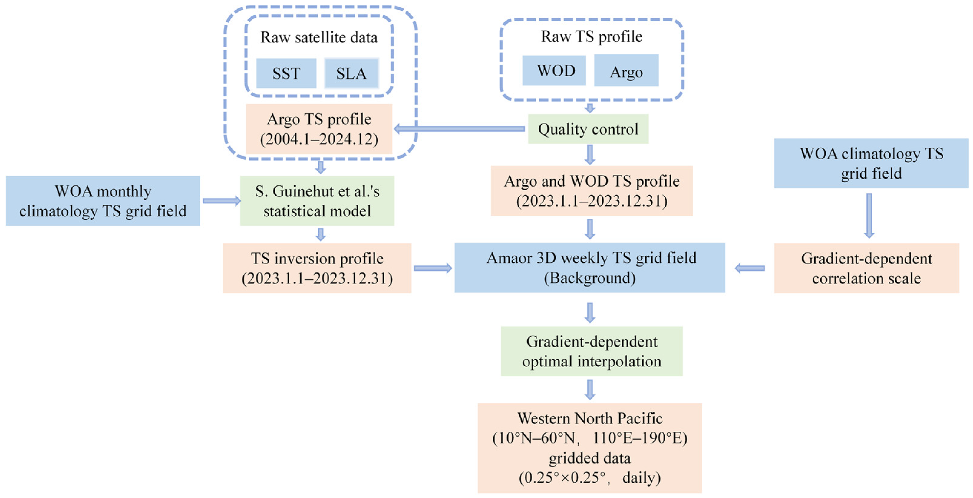
The multi-source data fusion method mainly includes the collection and quality control of historical observational profiles, the inversion of temperature and salinity profiles based on surface observations and Argo observations, multi-source data fusion, and derivative factor calculation, among other steps. Firstly, range detection, peak detection, and density detection of temperature and salinity were used for quality control of multi-source observational data. Then, based on Argo profiles of temperature and salinity, satellite sea surface observations, and a statistical model, the monthly climatology of World Ocean Atlas 2023 (WOA23) with a spatial resolution of 0.25° was used as the initial background field to invert the daily profiles of temperature and salinity. Then, after calculating the gradient-dependent correlation scale, the Armor-3D weekly analysis field was used as the initial field to fuse the inverted profiles, as well as Argo, WOD, and other observational data (Figure 2), to reconstruct the three-dimensional dataset (Gradient-Dependent Correlation Scale Method Version 3, GDCSMV3) using the gradient-dependent optimal interpolation objective analysis method. Finally, the geostrophic currents were calculated from temperature and salinity.

4.1. Validation of Inverted Profiles

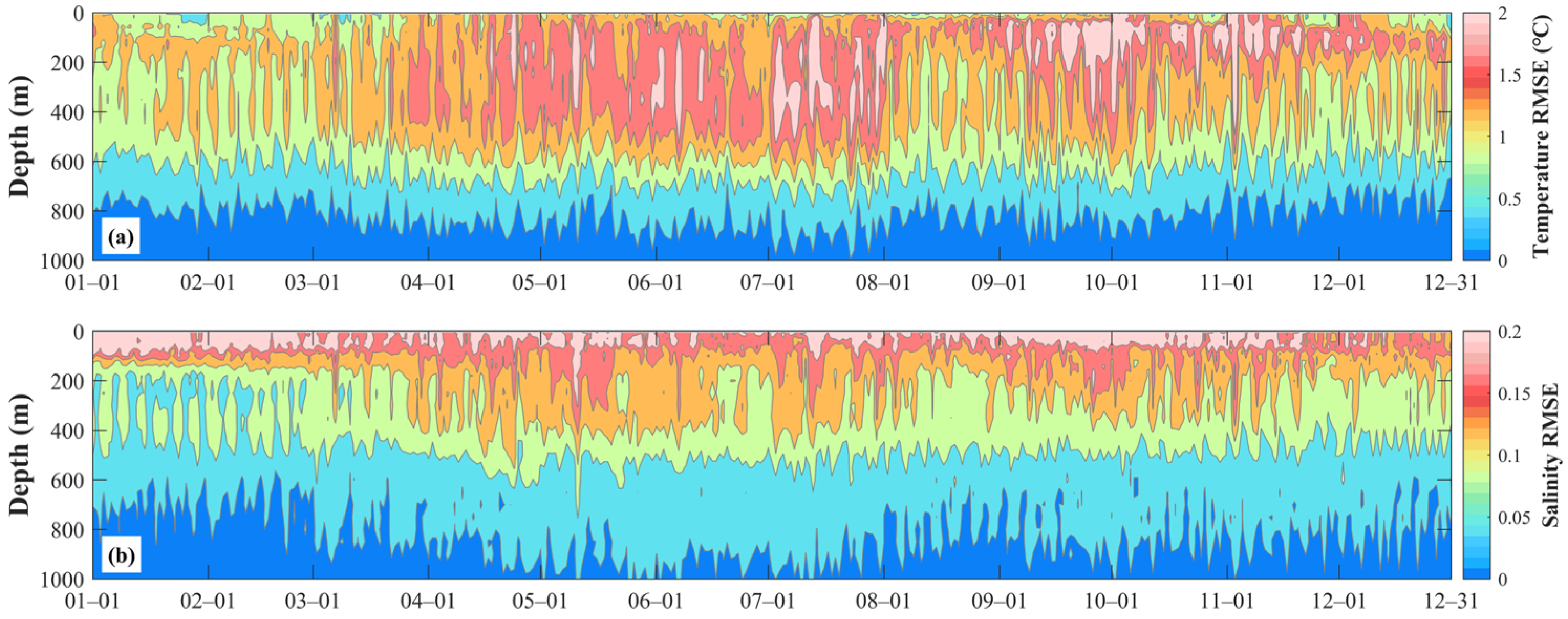
In this section, the accuracy of the inverted profiles is assessed by calculating the root mean square errors (RMSEs) and comparing them with the observed profiles. The time series of the temperature and salinity RMSEs of inverted profiles relative to the Argo observations in the upper 1000 m from 1 January 2004 to 31 December 2024 are shown in Figure 3. As shown in the figure, the high RMSE of temperature is mostly concentrated at depths of 200–500 m, and the maximum is less than 2 °C. The maximum RMSE of salinity is below 0.2, and the RMSE gradually decreases with increasing depth. Before 1 April, the RMSEs of temperature and salinity are relatively small. The RMSE of temperature is less than 1 °C, and the RMSE of salinity below 200 m is less than 0.1. From April to August, the RMSE is relatively large, and the average RMSEs of temperature and salinity below 600 m are about 1.5 °C and 0.15, respectively. The RMSEs of temperature and salinity from August to December decrease again, and there is a large value in the upper 200 m. The RMSEs of temperature and salinity below 600 m are low, at less than 0.5 °C and 0.05, respectively.
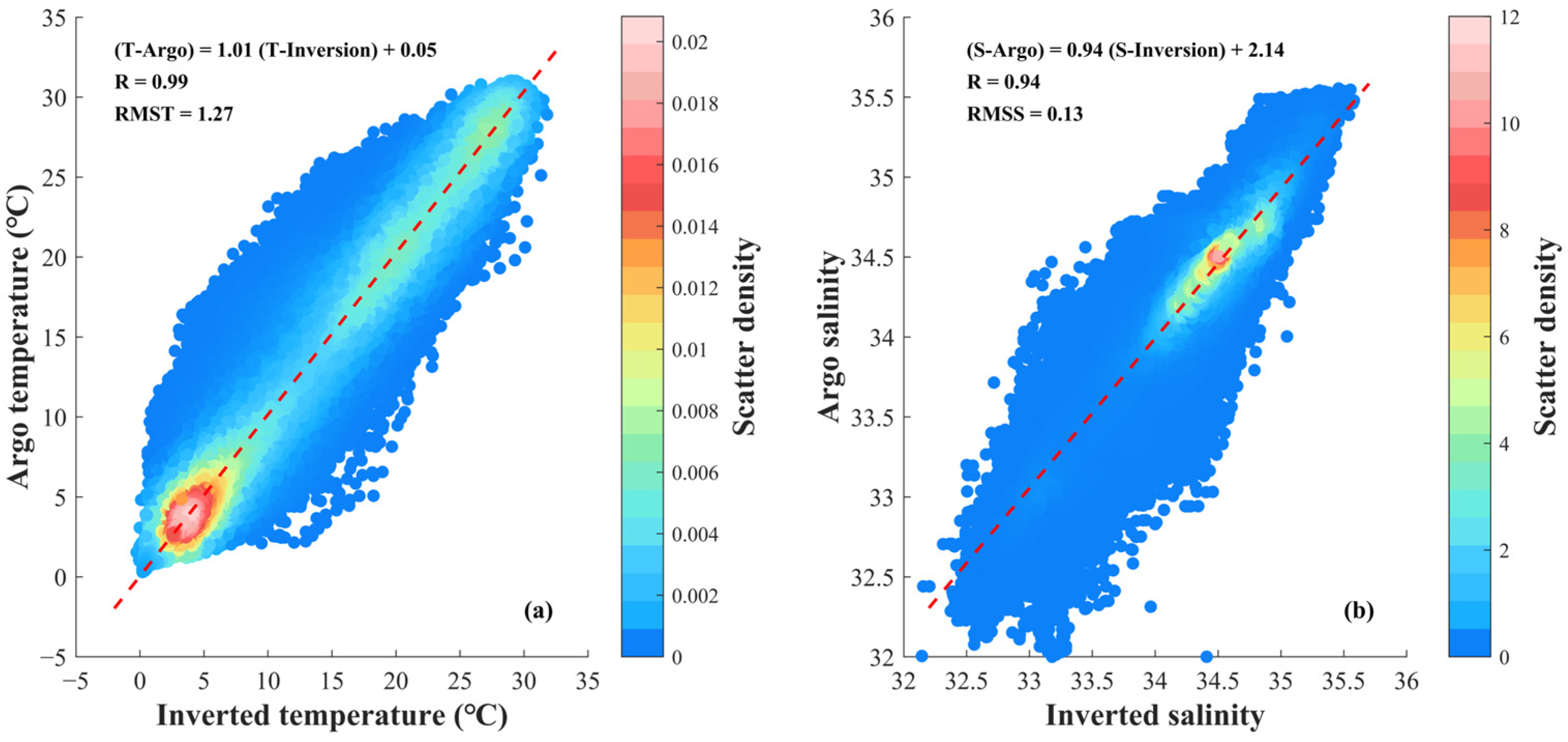
The scatter density distribution between the inverted profiles and the Argo observations is shown in Figure 4. The temperature and salinity scatter distributions of the inverted profiles and Argo observations are relatively concentrated. The correlation coefficients of temperature and salinity are as high as 0.99 and 0.94, and the overall average RMSE values are 1.27 °C and 0.13, respectively. There is an obvious linear relationship between the inverted profiles and the Argo observations. The high-probability density scatters are concentrated on both sides of the fitting curve, and the corresponding linear fitting slopes for temperature and salinity are 1.01 and 0.94, respectively. This indicates that, under high-probability statistics, the inverted profiles have strong consistency with the Argo observations.
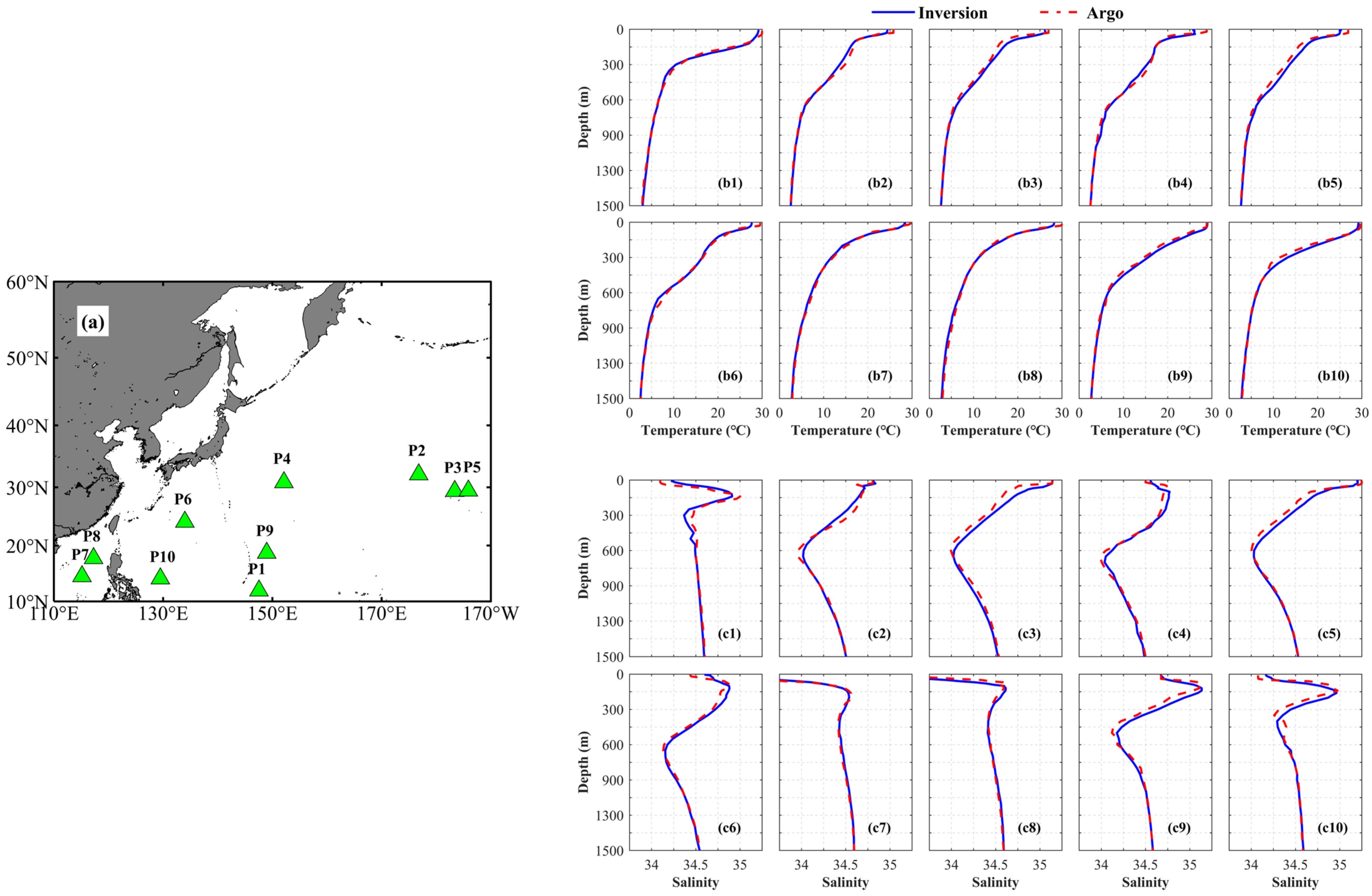
The comparison results of 10 Argo observational profiles and inverted profiles on 1 October 2023 are shown in Figure 5. Overall, the inverted profiles of temperature show a relatively consistent vertical variation trend with the Argo observational profiles; in particular, the temperature decreases gradually with increasing depth, the mixed layer and the thermocline structure are obvious, the mixed layer depth is mainly shallower than 100 m, and the thermocline is mainly distributed shallower than 150 m (Figure 5(b1–b6)). In addition, the maximum temperature differences between the inverted profiles and the Argo observational profiles are less than 1.5 °C. The maximum differences are concentrated in the surface layer and the thermocline near 200 m, and the temperature differences below 200 m are mostly less than 0.5 °C. In comparison, the vertical variation in salinity is complex, but the maximum differences in different profiles appear at the same depth. The largest differences for most profiles appear in the subsurface layer, and the maximum differences in some profiles appear at 200 m or 500 m with a dramatic change in salinity. However, the vertical variations in all inverted profiles are very similar to those in the Argo observational profiles, and the salinity difference below 600 m is within 0.02. In summary, the inverted profiles reproduce the temperature and salinity distribution inside the ocean, and the differences exist within a controllable range.

4.2. Parameter Set for Data Fusion

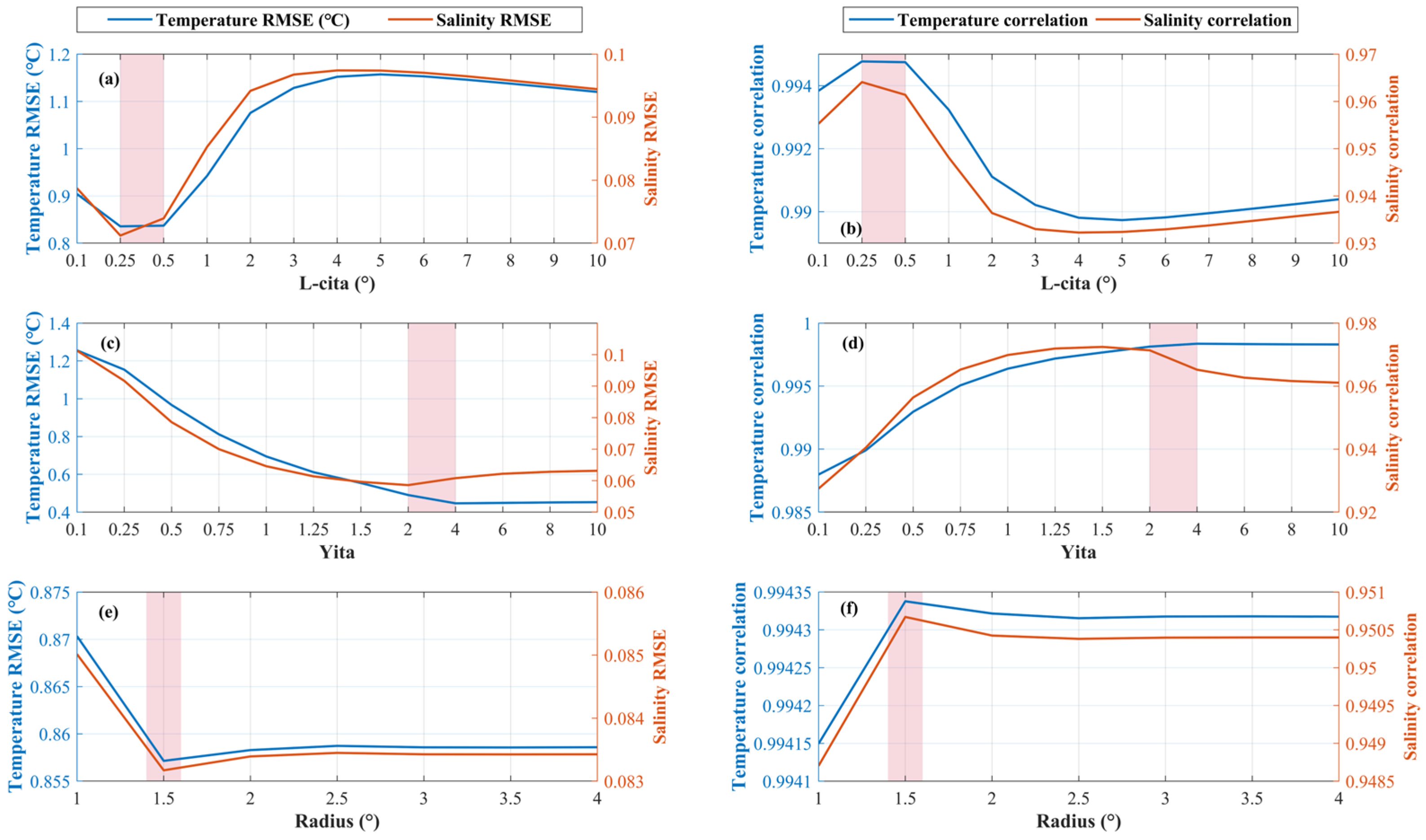
In this study, the gradient-dependent optimal interpolation method was used to reconstruct the high-resolution gridded dataset GDCSMV3. The search radius in longitude and latitude, the correlation scale constant L-cita, and the dimensionless relative observation error constant Yita (observation/background error) affect the reconstructed results. Reasonable settings were needed to obtain the best reconstructed results. The RMSEs and correlation coefficients of the reconstructed results relative to the observational data varied within different parameters, as shown in Figure 6. The results of temperature and salinity have a similar change. With the increase in the L-cita, the RMSE of the reconstructed results decreases first and then increases, reaching a minimum at the L-cita of 0.25 (Figure 6a), while the correlation coefficient increases first and then decreases, approaching 0.995 at the L-cita of 0.25 (Figure 6b). As the Yita increases, the RMSE gradually decreases. When the Yita is greater than 2, the RMSE tends to stabilize, the corresponding correlation coefficient gradually increases, and the RMSE reaches an extremum when the Yita is 2 (Figure 6c,d). As the search radius increases, the RMSE decreases first and then increases, while the correlation coefficient shows the opposite pattern, with a significant extreme value at 1.5° (Figure 6e,f). In summary, this study used a correlation scale constant of 0.25°, a relative observation error constant of 2, and a search radius of 1.5° to reconstruct the dataset.

5. Results

5.1. Theoretical Verification

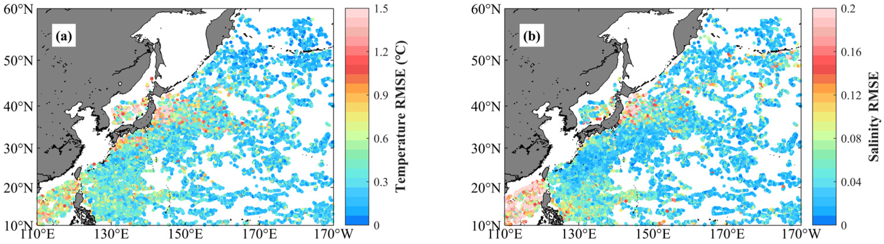
Using the selected parameters (correlation scale constant of 0.25°, relative observation error constant of 2, and search radius of 1.5°), the RMSE scatter distributions of the 2023 daily average reconstructed results of temperature and salinity relative to the Argo and WOD observations are shown in Figure 7. The RMSE of temperature (Figure 7a) is generally below 0.6 °C. Only in the South China Sea, the Sea of Japan, and the east coast of Japan, the RMSEs of temperature are relatively high, but the maximum is still within 1.2 °C. The distribution of salinity RMSE is similar to that of temperature and remains below 0.08 (Figure 7b). The larger RMSEs are distributed in the South China Sea and the northeastern coast of Japan, which are related to sparse observational data in nearshore regions and the optimal weight calculation method of the objective analysis scheme at the land and sea boundary. Except for the western boundary, the RMSEs of temperature and salinity in the open sea area are mostly lower than 0.5°C and 0.05.
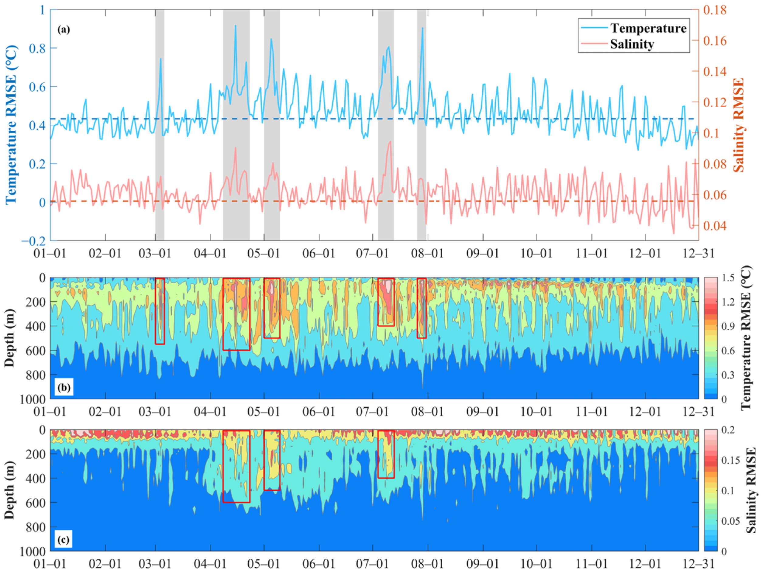
The time series of the RMSEs of temperature and salinity between the reconstructed results and the Argo and WOD observations are shown in Figure 8. The temperature RMSEs of the reconstructed results are between 0.19 °C and 0.92 °C, and the average RMSE is 0.43 °C. The salinity RMSEs are between 0.022 and 0.100, and the average RMSE is 0.056 (Figure 8a). As shown in the vertical section (Figure 8b), the RMSE of temperature increases first and then decreases with increasing depth. Before 1 April, the RMSE of temperature is mostly below the mean value with a small range variation and the maximum is below 0.8 °C. The larger RMSE is distributed shallower than 600 m, and the maximum is less than 1 °C. The high RMSE of temperature from April to August is between 0.4 °C and 1 °C, and the RMSE below 600 m is also controlled below 1.5 °C. From August to December, the RMSE of temperature fluctuates around the mean value, and the overall RMSE is between 0.3 °C and 0.6 °C. There is no large RMSE during this period. The RMSE of salinity shows a decreasing trend with increasing depth (Figure 8c) and fluctuates around the mean value in 2023. There are only large RMSEs on 15 April, 5 May, and 8 July, but the RMSEs are controlled below 0.1. In summary, the RMSEs of the reconstructed results are generally good. Although there are large RMSEs on some dates, they remain within a reasonable range.

5.2. Comparison with Other Datasets

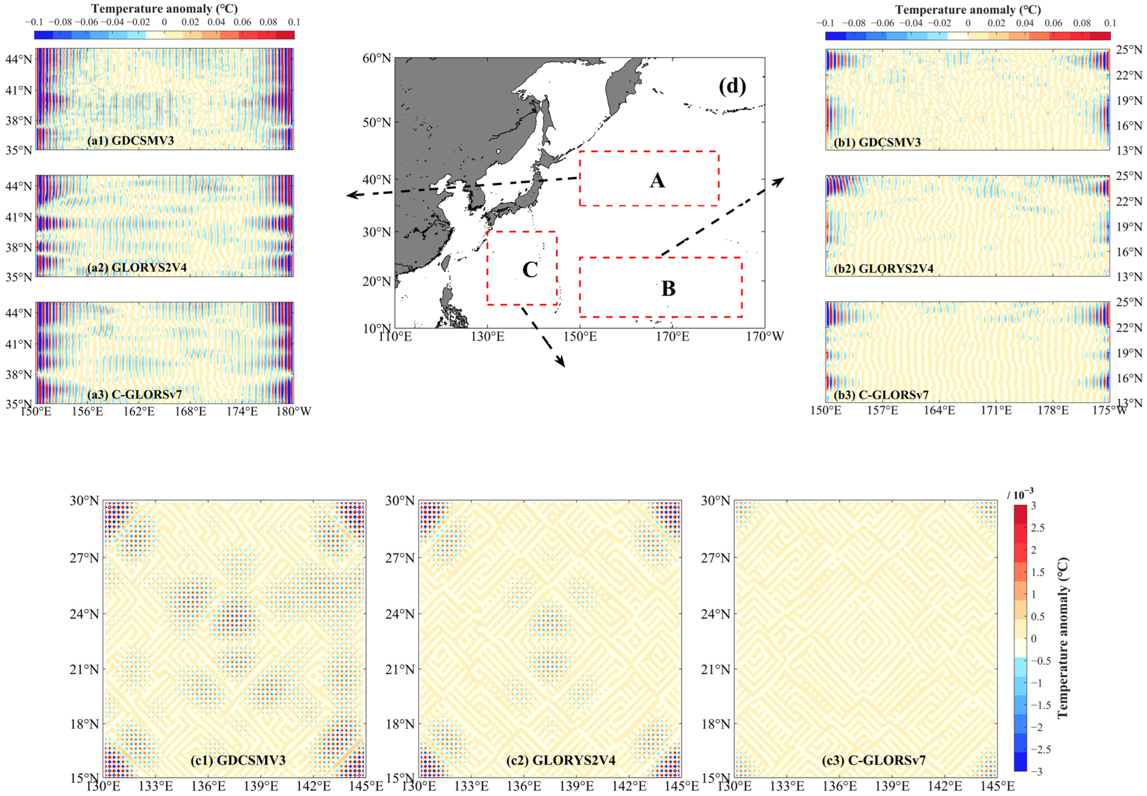
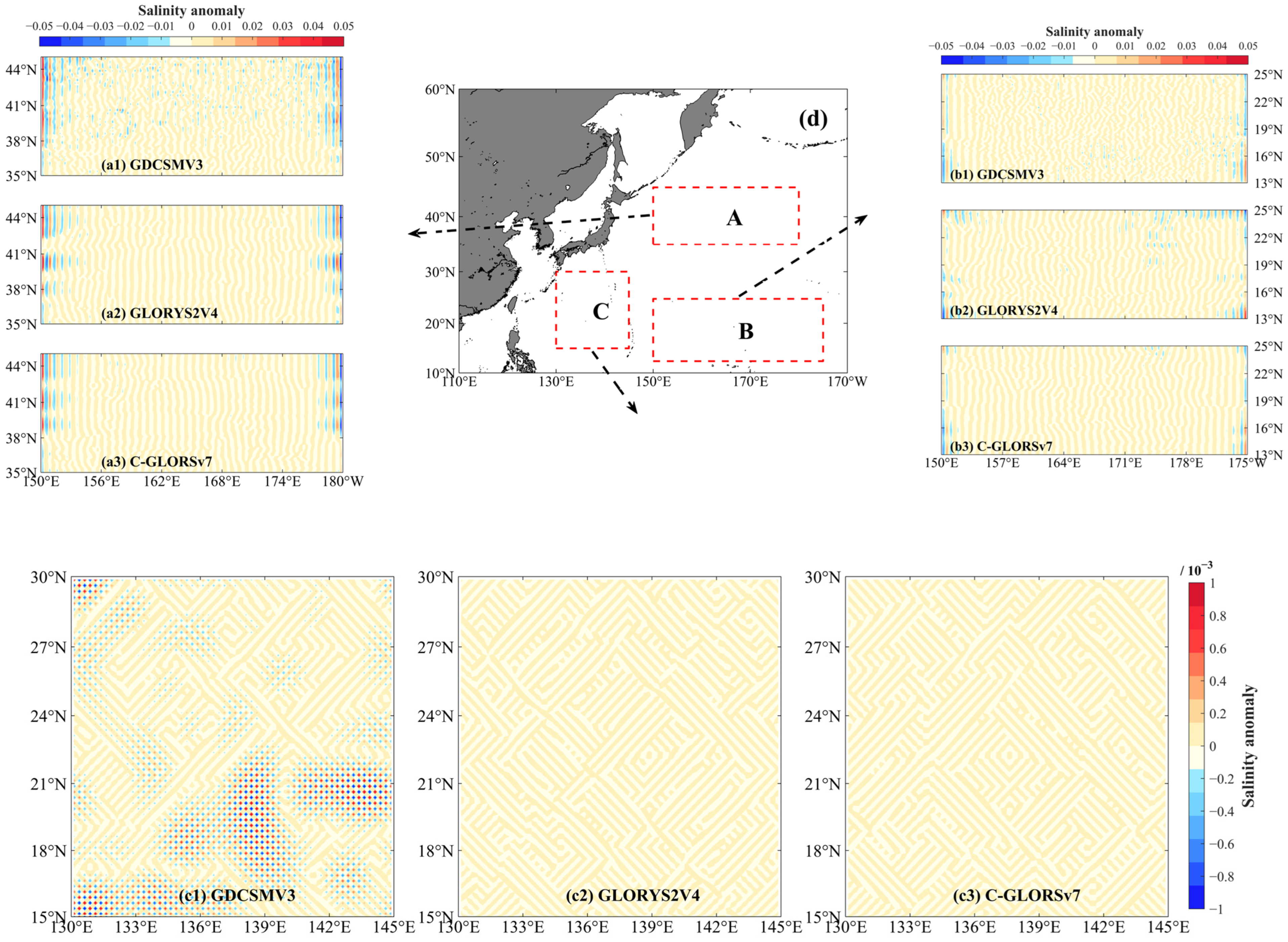
To examine the ability of the reconstructed result GDCSMV3 to extract ocean high-frequency signals, the mesoscale and small-scale signals of GDCSMV3, GLORYS2V4, and C-GLORSv7 were analyzed based on the fast Fourier transform [22], ideal high-pass filtering [32], and the temperature and salinity anomaly fields. The temperature and salinity anomaly fields of the Kuroshio Extension (150° E–180° E, 35° N–45° N, region A), the southeast sea area (150° E–185° E, 13° N–25° N, region B) and the southwest offshore sea area (130° E–145° E, 15° N–30° N, region C) at 100 m on 1 October 2023 were extracted via Fourier transform. After the frequency domain information was extracted, the low-frequency signals within 40 steps from the origin were removed by the filter. Finally, the temperature and salinity anomaly fields were obtained using the inverse Fourier transform. The temperature anomaly distribution is shown in Figure 9. The high values of temperature anomalies in the three datasets are densely distributed at the edges due to noise in spectral analysis. Among them, region A is the intersection area of cold and warm water, and the temperature changes sharply. The corresponding high-frequency signals of temperature anomaly present a zonal distribution in the latitudinal direction and cover almost the whole area. Region B is dominated by large-scale advection, and the high-value distribution of temperature anomaly is relatively sparse and concentrated to the north of the region. Region C, as a strong current region, is close to the western boundary. The high values of the temperature anomaly corresponding to the spectrum analysis diffuse around the center of the region, and the high-frequency signals are patchy. For different datasets, whether at the edge or the center of the region, the high-value distribution of GDCSMV3 temperature anomaly in region A is more concentrated, especially between 38° N and 41° N. The temperature anomaly distributions of GLORYS2V4 and C-GLORSv7 are similar. However, the continuity of high-frequency signals at the boundary is significantly lower than in GDCSMV3, and the range of high-frequency bands in the middle is also significantly reduced. Both GDCSMV3 and GLORYS2V4 have many high-temperature anomalies north of 19° N in region B, while C-GLORSv7 has relatively few high-frequency signals. In region C, the temperature anomalies of GDCSMV3 and GLORYS2V4 have dense high values around the region. Moreover, GDCSMV3 has not only stronger temperature anomalies but also almost full coverage of temperature anomalies east of 142° E, while the high-frequency signals of C-GLORSv7 across the whole region are significantly weakened.
In comparison, the spatial distribution of salinity anomaly shows significant differences (Figure 10). Overall, the high-value coverage area of salinity results is much smaller than temperature. The high-frequency signals of salinity in region A are mainly concentrated north of 38° N. The high-salinity anomaly of GDCSMV3 is distributed in spots between 38° N and 44° N, while GLORYS2V4 and C-GLORSv7 have high-frequency salinity changes only in the edge region. The high-frequency signals of the salinity spectrum analysis of the three datasets in region B are relatively weak. GDCSMV3 is similar to GLORYS2V4, and C-GLORSv7 is the weakest. The high value of the GDCSMV3 salinity anomaly in region C is mainly distributed south of 22° N and the distribution is concentrated. There are almost no high-salinity anomalies in GLORYS2V4 and C-GLORSv7 relative to GDCSMV3.
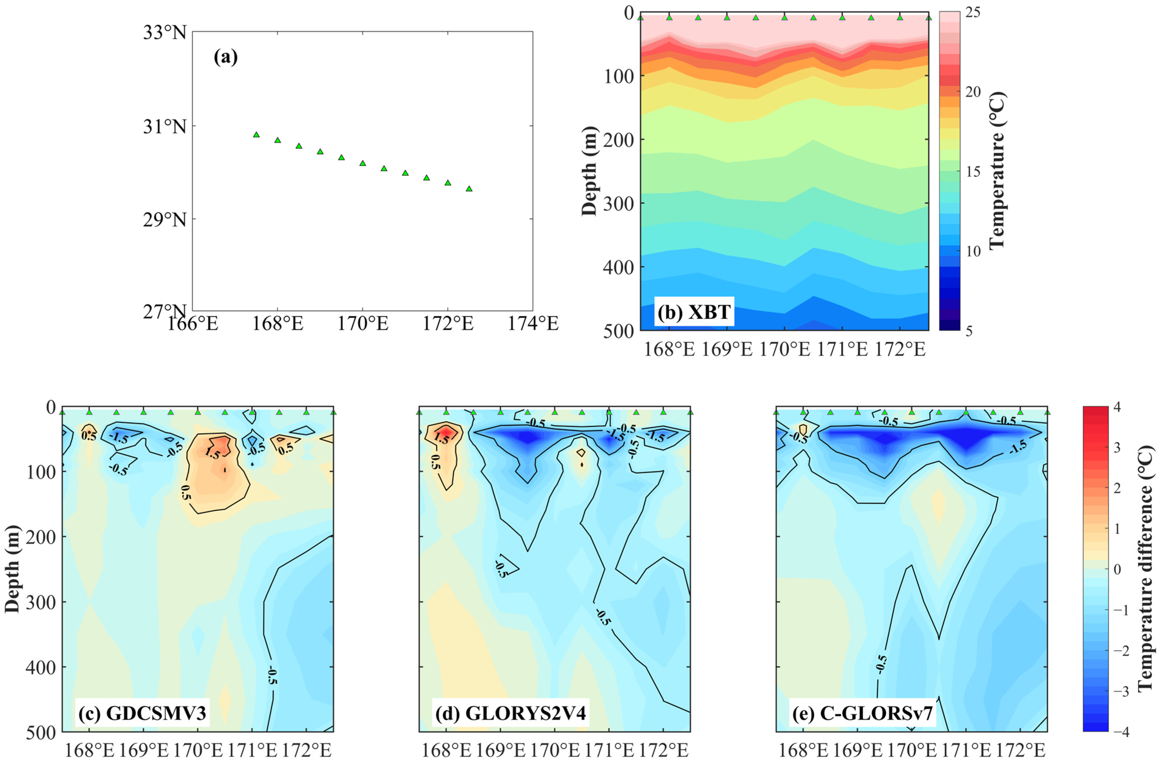
Figure 11 shows eleven XBT observational profiles of temperature on 13 October 2023, to compare and verify the accuracy of GDCSMV3. The location of the XBT stations is shown in Figure 11a, and the latitude differences among the stations are small, so a latitudinal section is drawn to analyze the temperature difference. Vertically, as depth increases, the temperature differences for different datasets relative to XBT increase first and then decrease. The larger difference (±1.5 °C) is mainly concentrated at depths of 50–100 m, where the temperature changes dramatically (Figure 11b). Latitudinally, the temperature of the three datasets alternately appear as positive and negative differences from west to east, and the high differences are mainly concentrated at the three stations at 168° E, 169° E, and 171° E. The temperature differences for GDCSMV3 at these three stations are mostly between 0.5 and 1.5 °C, and the influence depth where differences are greater than 1.5 °C is less than 50 m. Meanwhile, the ±1.5 °C isolines of GLORYS2V4 and C-GLORSv7 cover almost all areas shallower than 100 m. Below 200 m, the temperature differences for GDCSMV3 are mostly below 0.5 °C, exceeding 0.5 °C at only a few (about three) stations east of 171° E, while the ±0.5 °C isolines of GLORYS2V4 and C-GLORSv7 extend to 300 m and 500 m, respectively, and the temperature differences at all seven stations east of 169° E exceed 0.5 °C.
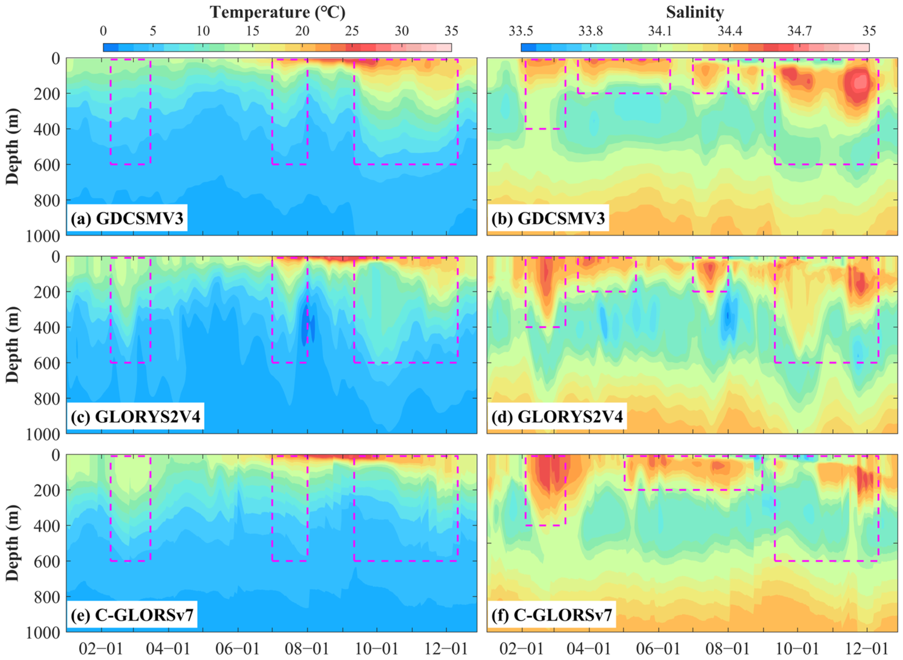
Time–depth distributions of reconstructed temperature and salinity at the station (38° N, 153° E) in 2023 show that the variation trends of temperature and salinity at different depths are similar across the three datasets (Figure 12). The temperature and salinity of GDCSMV3 change relatively gently, while those of GLORYS2V4 and C-GLORSv7 are more intense. For example, from 9 February to 15 March, from 1 to 31 July, and from 10 September to 10 December, during the thickening of the warm water layer below 400 m, the isolines of the GDCSMV3 temperature section change smoothly, and the sinking depths of the warm water are about 400 m, 400 m, and 600 m, respectively. The temperature isoline of C-GLORSv7 changes more dramatically than that of GDCSMV3, and the warm water layer from 9 February to 15 March exceeds 500 m. The temperature change for GLORYS2V4 is the most severe, and the influence depths of the warm water layer in the three periods are more than 500 m. The salinity of the three datasets decreases first and then increases with increasing depth. There is an obvious low salinity core at 300–600 m, and the variation trend of salinity isolines over time is also consistent. However, the influence depth of the high-salinity core above 400 m is quite different: from early February to mid-August, the subsurface high-salinity range of GDCSMV3 is less than 200 m and the salinity changes little over time. In contrast, GLORYS2V4 and C-GLORSv7 show the opposite pattern: the influence depths of the subsurface high salinity core are up to 400 m, and the salinity changes sharply with time. For the high-salinity cores from early September to early December, GDCSMV3 is more significant than the others and has a greater depth of influence. In addition, regardless of temperature or salinity, the continuity of the GDCSMV3 result is significantly stronger than those of GLORYS2V4 and C-GLORSv7.

6. Discussion

6.1. Identification of Kuroshio Path

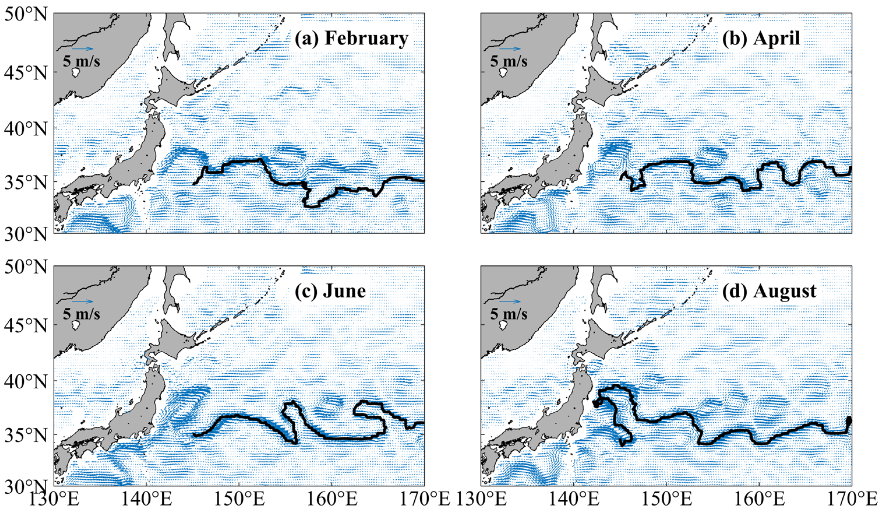
The Kuroshio path is an important feature of the large-scale dynamic processes in the Northwest Pacific Ocean. In this study, the geostrophic currents were calculated from the GDCSMV3 temperature and salinity data. Then, the Kuroshio path identification method was used to explore the ability of GDCSMV3 to characterize the large-scale motion characteristics using the flow field at 100 m on 5 February, April, June, and August 2023, as an example. The Kuroshio path shown in Figure 13 starts from the point (145° E, 35° N) and mainly extends from west to east along the latitude band from 35°N to 38°N. It swings zonally with seasonal variation and is accompanied by vertical structure adjustment, which is consistent with previous studies [33,34]. Specifically, the Kuroshio path at 100 m in February is located east of 150° E and shifts southward to 32° N due to the influence of strong eddy motion. In April, the subtropical high moves northward, and the Kuroshio path begins to rise northward. In June, the Kuroshio path continues to move northward, up to 38° N. Due to intensified eddy–current interactions at 160° E, a protruding path is formed. During the period of a strong warm water tongue in August, the velocity of 100 m layer increases, and the northward protruding path extends to the northwest shelf area.

6.2. Identification of Mesoscale Eddy

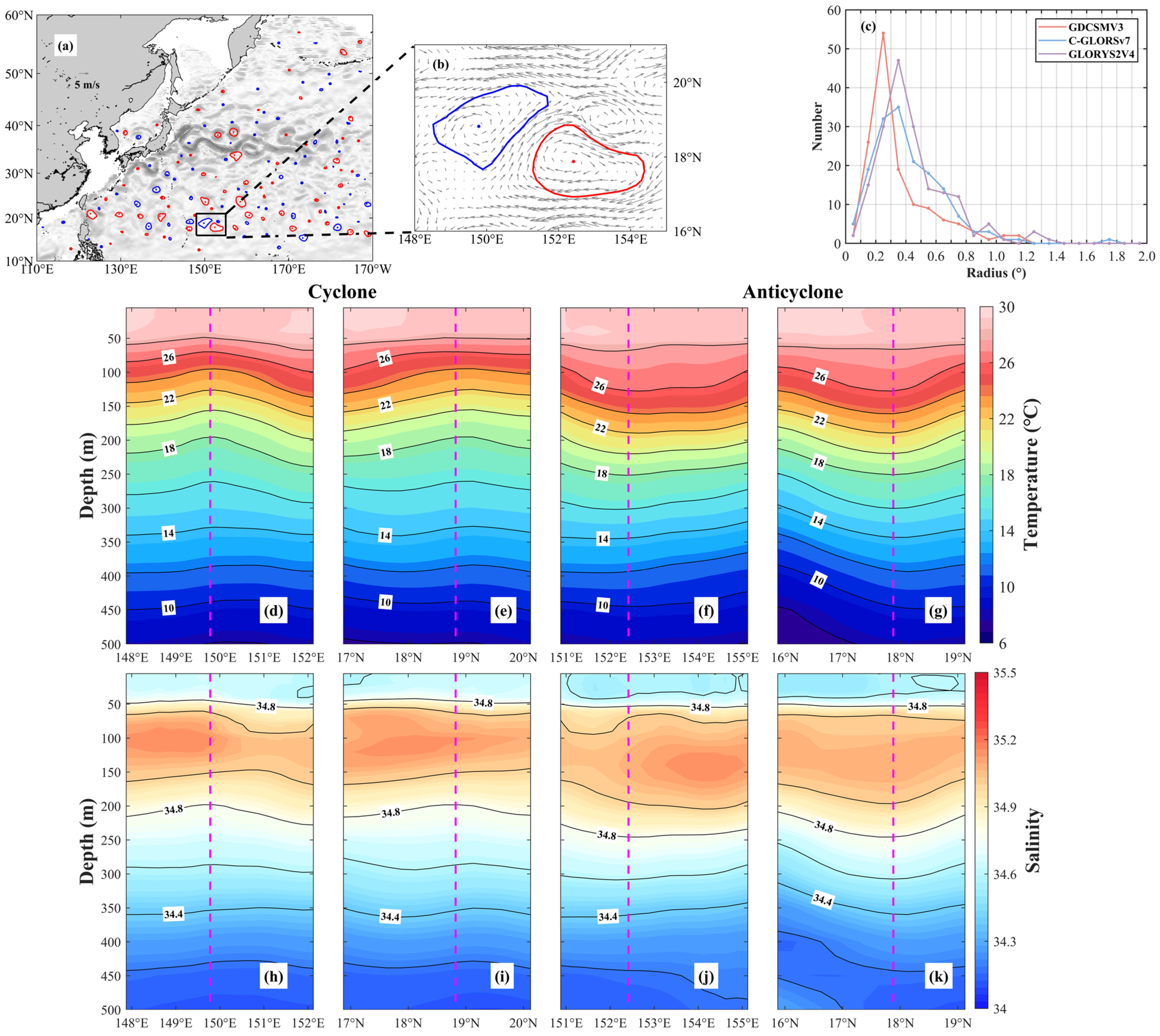
Although the 0.25° spatial resolution of GDCSMV3 cannot reach eddy resolution, the advantage of gradient-dependent optimal interpolation is that it can retain mesoscale information in the observation data as much as possible. As shown in Figure 14, the geostrophic currents were calculated first and then the flow vector method was used to perform mesoscale eddy detection experiments on the current field at 100 m on 1 October 2023. An eddy pair in the region (148° E–155° E, 16° N–21° N) was selected (Figure 14b) and the meridional and zonal temperature and salinity sections of the eddy center were plotted (Figure 14d–k). Finally, a total of 139 mesoscale eddies were detected, including 73 cyclonic eddies and 66 anticyclonic eddies. The eddies are mostly distributed south of 40° N, and the detected mesoscale eddies have a wide range of influence radius. Compared to GLORY2V4 and C-GLORSv7, GDCSMV3 has a higher number of eddies within a 0.4° eddy radius. This indicates that GDCSMV3 has a good ability to characterize large-scale strong eddies and small-scale weak eddies. In addition, the temperature and salinity sections inside the cyclonic eddy shown in Figure 14d,e,h,i indicate that, due to the counterclockwise rotation of seawater inside the cold eddy and the combined effect of the Coriolis force, seawater accumulates at the edge of the eddy. As a result, the low-temperature seawater in the eddy center rises from bottom to top, especially at the center. Similarly, Figure 14f,g,j,k show that the high-temperature and high-salinity water sinks inside the anticyclonic eddy. In addition, the upwelling of seawater in the center of the cyclone eddy causes the high-salinity core of 50–150 m to transport to both sides of the eddy center, and the sinking of the anticyclonic eddy causes the high-salinity core to gather to the eddy center. This is clearly reflected in the salinity section of the GDCSMV3 (Figure 14h–k).

7. Conclusions

Satellites and Argo provide global ocean temperature and salinity information at a high rate every year. However, there are few data products with high spatial and temporal resolution providing multiple ocean variables produced through the effective fusion of multi-source data. Based on the observation data itself, this study constructed a data fusion framework for high-resolution regional dataset in the Northwest Pacific. Firstly, the subsurface temperature and salinity profiles were inverted using a statistical parameter model based on the satellite sea surface observational data. Then, the inverted profiles, Argo profiles, historical observations, and other multi-source data were fused to construct the daily average three-dimensional temperature and salinity dataset (GDCSMV3) of the Northwest Pacific Ocean (110° E–190° E, 10° N–60° N) from 1 January 2023 to 31 December 2023 based on the gradient-dependent optimal interpolation method. The accuracy and reliability of GDCSMV3 were verified through a theoretical test, spectral analysis, measured comparisons, and analogy tests.
The statistical parameter model based on linear regression conveniently and quickly established the statistical relationship between the ocean surface and the internal environment information and improved the space–time observation density inside the ocean through satellite sea surface observation. The temperature RMSE of the inverted profiles relative to the Argo profiles is below 2 °C, and the salinity RMSE is less than 0.2. With increasing depth, the RMSEs of temperature and salinity gradually decrease. In 2023, the RMSEs of temperature and salinity are low before April. From April to August, the RMSEs below 600 m are relatively high, and decrease after August. In addition, in terms of correlation coefficients, the inverted profiles and the Argo profiles show strong consistency in temperature and salinity. The correlation coefficients of temperature and salinity are 0.99 and 0.94, respectively, and the overall average RMSEs are about 1.27 °C and 0.13, respectively.
The gradient-dependent optimal interpolation method can automatically adjust the optimal weights of various data sources according to the spatial and temporal resolution and relative accuracy of the observed data, so that the fusion results retain as much of the original information in the data as possible. The key parameters in this method, such as search radius in longitude and latitude, correlation scale constant, and dimensionless relative observation error, need to be tested and adjusted according to the observation density and spatiotemporal resolution of the fusion region. In the Northwest Pacific Ocean, using a search radius of 1.5°, a correlation scale constant of 0.25°, and a relative observation error of 2 to construct a daily dataset with a spatial resolution of 0.25° is the optimal choice (the construction result error is the smallest).
Based on this parameter selection, the temperature RMSE of the dataset constructed by the fusion of multi-source data relative to the measured data is basically within 1.2°C, the salinity RMSE is within 0.08, and the high RMSE values are mostly distributed in the South China Sea and the East Coast of Japan, among other boundary areas. During 2023, the overall RMSE of temperature was between 0.19 and 0.92 °C, and the average RMSE was 0.43 °C. The RMSE of salinity was between 0.022 and 0.100, and the average RMSE was 0.056. The spectral analysis results show that GDCSMV3 temperature and salinity fields exhibit stronger high-frequency signals than those of GLORYS2V4 and C-GLORSv7. Compared with the measured temperature of XBT, the overall average temperature difference in GDCSMV3 is the smallest, and the difference ranges of ±1.5 °C and ±0.5 °C are smaller than those of the other datasets. In the temporal and spatial sections of typical stations, the temperature and salinity changes in the three data products are consistent, but GDCSMV3 has a more significant high-temperature core and high-salinity core, and the influence depth is greater. In addition, GDCSMV3 clearly shows the zonal swings of the Kuroshio path with seasonal variation, as well as the internal temperature and salinity structural characteristics of typical mesoscale eddy pairs.
In view of the spatial and temporal density of the current observational data, and to ensure the accuracy of the data fusion effect as much as possible, this study constructed only a daily fusion product with a spatial resolution of 0.25°. Although the data failed to reach eddy resolution (1/12°), based on the density flow field, 139 mesoscale eddies were identified by the flow vector method, which cover almost the entire Northwest Pacific Ocean. Compared to GLORY2V4 and C-GLORSv7, GDCSMV3 has a higher number of eddies within a 0.4° eddy radius. GDCSMV3 shows the upwelling and sinking of seawater inside the eddies, as well as the fine structure of temperature and salinity. This indicates that it can provide important data support for studying the real-time evolution of mesoscale processes and their impact on local hydrology and the ecological environment. In addition, considering computational efficiency, this study uses only the data from one year (2023) as an example for analysis and discussion (Table A1 and Table A2). The construction of long-term sequence datasets can be updated regularly according to the needs of research.

Author Contributions

L.F.: Writing—original draft, Conceptualization, Formal analysis, Investigation, Software, Validation. C.Z.: Writing—original draft, Writing—review & editing, Conceptualization, Methodology, Software, Supervision, Validation. Y.G.: Writing—original draft, Writing—review & editing, Conceptualization, Supervision, Validation. B.S.: Writing—review & editing, Data curation. R.Z.: Writing–review & editing, Formal analysis. All authors have read and agreed to the published version of the manuscript.

Funding

This study was funded by the Program on the Survey, Monitoring and Assessment of Global Fishery Resources (Comprehensive scientific survey of fisheries resources at the high seas) sponsored by the Ministry of Agriculture and Rural Affairs (No. D-8025-25-5001) and the project supported by the General Program of the National Natural Science Foundation of China (Grant No.42576203).

Data Availability Statement

The post-quality-controlled Argo dataset from China Argo Real-Time Data Center is available at https://www.argo.org.cn/ (accessed on 21 May 2025). The WOD profile data can be accessed at https://www.ncei.noaa.gov/products/world-ocean-database (accessed on 21 May 2025). The daily sea level anomaly product (Global Ocean Gridded L4 Sea Surface Heights And Derived Variables Reprocessed Copernicus Climate Service) is available at https://data.marine.copernicus.eu/product/SEALEVEL_GLO_PHY_CLIMATE_L4_MY_008_057/description (accessed on 19 May 2025) and the multi-year climatology sea level anomaly product (Global Ocean Mean Sea Level trend map from Observations Reprocessing) is available at https://data.marine.copernicus.eu/product/OMI_CLIMATE_SL_GLOBAL_regional_trends/description (accessed on 21 May 2025). The weekly temperature and salinity three-dimensional dataset (Multi Observation Global Ocean ARMOR3D L4 analysis) is downloaded from https://data.marine.copernicus.eu/product/MULTIOBS_GLO_PHY_TSUV_3D_MYNRT_015_012/description (accessed on 30 June 2025) and the daily temperature and salinity three-dimensional dataset (Global Ocean Ensemble Physics Reanalysis) is available at https://data.marine.copernicus.eu/product/GLOBAL_MULTIYEAR_PHY_ENS_001_031/description (accessed on 21 July 2025). The daily sea surface temperature product can be accessed at https://psl.noaa.gov/data/gridded/data.noaa.oisst.v2.highres.html (accessed on 18 June 2025) and the World Ocean Atlas 2023 (WOA23) climatology product is available at https://www.ncei.noaa.gov/products/world-ocean-atlas (accessed on 21 May 2025).

Acknowledgments

I would like to express my sincere gratitude to my supervisor for the valuable guidance she provided for this article. Thanks are extended to the China Argo Real-Time Data Center for providing the data source (ftp://ftp.argo.org.cn/pub/ARGO/global/, accessed on 21 May 2025).

Conflicts of Interest

The authors declare no conflicts of interest.

Appendix A

Table A1. Computer configuration.
ComponentsModel
CPU (central processing unit)Intel (R) Core(TM) i7-10700 CPU @ 2.90 GHz, 2901 Mhz, octa
RAM (random access memory)32 GB
Table A2. Time required to reconstruct 1-day data.
ProcessTime (Seconds)
Inversion of T/S profiles100.104
Data fusion53.007

References

  1. Lehman, J. Sea Change: The World Ocean Circulation Experiment and the Productive Limits of Ocean Variability. Sci. Technol. Hum. Values 2020, 46, 839–862. [Google Scholar] [CrossRef]
  2. Moltmann, T.; Turton, J.; Zhang, H.M.; Nolan, G.; Gouldman, C.; Griesbauer, L.; Willis, Z.; Piniella, Á.M.; Goldstraw, S.; Barrell, S.; et al. A Global Ocean Observing System (GOOS), Delivered Through Enhanced Collaboration Across Regions, Communities, and New Technologies. Front. Mar. Sci. 2019, 6, 291. [Google Scholar] [CrossRef]
  3. Liu, Q.; Bao, S.; Yan, H.; Wang, H.; Wang, Y.; Ren, Z. Enhancing sea surface salinity short-term prediction using physically informed deep learning. Appl. Ocean Res. 2025, 165, 104832. [Google Scholar] [CrossRef]
  4. Good, S.; Fiedler, E.; Mao, C.; Martin, M.J.; Maycock, A.; Reid, R.; Roberts-Jones, J.; Searle, T.; Waters, J.; While, J.; et al. The Current Configuration of the OSTIA System for Operational Production of Foundation Sea Surface Temperature and Ice Concentration Analyses. Remote Sens. 2020, 12, 720. [Google Scholar] [CrossRef]
  5. Meissner, T.; Wentz, F.J.; Manaster, A.; Lindsley, R.; Brewer, M.; Densberger, M. Remote Sensing Systems SMAP Ocean Surface Salinities [Level 2C, Level 3 Running 8-Day, Level 3 Monthly], Version 6.0 Validated Release; Remote Sensing Systems: Santa Rosa, CA, USA, 2024. [Google Scholar] [CrossRef]
  6. Taburet, G.; Sánchez-Román, A.; Ballarotta, M.; Pujol, M.I.; Legeais, J.-F.; Fournier, F.; Faugère, Y.; Dibarboure, G. DUACS DT2018: 25 years of reprocessed sea level altimetry products. Ocean Sci. 2019, 15, 1207–1224. [Google Scholar] [CrossRef]
  7. Mishonov, A.V.; Boyer, T.P.; Baranova, O.K.; Bouchard, C.N.; Cross, S.; Garcia, H.E.; Locarnini, R.A.; Paver, C.R.; Reagan, J.R.; Wang, Z.; et al. World Ocean Database 2023; Bouchard, C., Ed.; NOAA Atlas NESDIS 97; NOAA National Environmental Satellite, Data, and Information Service: Silver Spring, MD, USA; NOAA National Centers for Environmental Information: Asheville, NC, USA, 2024; 206p. [Google Scholar] [CrossRef]
  8. Sun, C.G. The Data Management System for the Global Temperature and Salinity Profile Programme. 2010. Available online: https://www.aoml.noaa.gov/phod/docs/Sun_Goni_TheDataManagement.pdf (accessed on 29 July 2025).
  9. Gandin, L.S. Objective analysis of meteorological field. Gidrometeorol. Izdatestvo 1963, 286. [Google Scholar]
  10. Kalman, R.E. A New Approach to Linear Filtering and Prediction Problems. J. Basic Eng. 1960, 82, 35–45. [Google Scholar] [CrossRef]
  11. Evensen, G. The Ensemble Kalman Filter: Theoretical formulation and practical implementation. Ocean Dyn. 2003, 53, 343–367. [Google Scholar] [CrossRef]
  12. Lorenc, A.C. Analysis methods for numerical weather prediction. Q. J. R. Meteorol. Soc. 1986, 112, 1177–1194. [Google Scholar] [CrossRef]
  13. Roemmich, D.; Gilson, J. The 2004–2008 mean and annual cycle of temperature, salinity, and steric height in the global ocean from the Argo Program. Prog. Oceanogr. 2009, 82, 81–100. [Google Scholar] [CrossRef]
  14. Good, S.A.; Martin, M.J.; Rayner, N.A. EN4: Quality controlled ocean temperature and salinity profiles and monthly objective analyses with uncertainty estimates. J. Geophys. Res.-Ocean. 2013, 118, 6704–6716. [Google Scholar] [CrossRef]
  15. Zhang, C.; Wang, D.; Liu, Z.; Lu, S.; Sun, C.; Wei, Y.; Zhang, M. Global Gridded Argo Dataset Based on Gradient-Dependent Optimal Interpolation. J. Mar. Sci. Eng. 2022, 10, 650. [Google Scholar] [CrossRef]
  16. Schmidtko, S.; Johnson, G.C.; Lyman, J.M. MIMOC: A global monthly isopycnal upper-ocean climatology with mixed layers. J. Geophys. Res.-Ocean. 2013, 118, 1658–1672. [Google Scholar] [CrossRef]
  17. Wijffels, S.E.; Gebbie, G.; Robbins, P.E. Resolving the Ubiquitous Small-Scale Semipermanent Features of the General Ocean Circulation: A Multiplatform Observational Approach. J. Phys. Oceanogr. 2024, 54, 2503–2521. [Google Scholar] [CrossRef]
  18. Forget, G.; Campin, J.-M.; Heimbach, P.; Hill, C.N.; Ponte, R.M.; Wunsch, C. ECCO version 4: An integrated framework for non-linear inverse modeling and global ocean state estimation. Geosci. Model Dev. 2015, 8, 3071–3104. [Google Scholar] [CrossRef]
  19. Chen, Y.; Bao, S.; Cao, Y.; Zhang, W.; Wang, H. The Yin-He Global Ocean Data Assimilation and Forecast System. Ocean-Land-Atmos. Res. 2025, 4, 0121. [Google Scholar] [CrossRef]
  20. Guinehut, S.; Dhomps, A.L.; Larnicol, G.; Le Traon, P.Y. High resolution 3-D temperature and salinity fields derived from in situ and satellite observations. Ocean Sci. 2012, 8, 845–857. [Google Scholar] [CrossRef]
  21. Hosoda, S.; Ohira, T.; Nakamura, T. A monthly mean dataset of global oceanic temperature and salinity derived from Argo float observations. JAMSTEC Rep. Res. Dev. 2008, 8, 47–59. [Google Scholar] [CrossRef]
  22. Palupi, I.R.; Raharjo, W.; Kiswanti, S. The Role of 2D Fast Fourier Transform and High Pass Filter in Regional and Residual Anomaly Separation in Gravity. IOP Conf. Ser. 2021, 873, 012017. [Google Scholar] [CrossRef]
  23. Huang, B.; Liu, C.; Banzon, V.; Freeman, E.; Graham, G.; Hankins, B.; Smith, T.; Zhang, H.-M. Improvements of the Daily Optimum Interpolation Sea Surface Temperature (DOISST) Version 2.1. J. Clim. 2021, 34, 2923–2939. [Google Scholar] [CrossRef]
  24. Mulet, S.; Rio, M.-H.; Mignot, A.; Guinehut, S.; Morrow, R. A new estimate of the global 3D geostrophic ocean circulation based on satellite data and in-situ measurements. Deep Sea Res. Part II Top. Stud. Oceanogr. 2012, 77–80, 70–81. [Google Scholar] [CrossRef]
  25. Riishøjgaard, L.P. A direct way of specifying flow-dependent background error correlations for meteorological analysis systems. Tellus A 1998, 50, 42. [Google Scholar] [CrossRef]
  26. Kalnay, E. Atmospheric Modeling, Data Assimilation and Predictability; Cambridge University Press: Cambridge, UK, 2002. [Google Scholar]
  27. Zhang, C.; Xu, J.; Bao, X.; Wang, Z. An effective method for improving the accuracy of Argo objective analysis. Acta Oceanol. Sin. 2013, 32, 66–77. [Google Scholar] [CrossRef]
  28. Zhang, C.; Wang, Z.; Liu, Y. An argo-based experiment providing near-real-time subsurface oceanic environmental information for fishery data. Fish. Oceanogr. 2021, 30, 85–98. [Google Scholar] [CrossRef]
  29. Stewart, R.H. Introduction to Physical Oceanography; Texas A&M University: College Station, TX, USA, 2008. [Google Scholar]
  30. Ambe, D.; Imawaki, S.; Uchida, H.; Ichikawa, K. Estimating the Kuroshio axis south of Japan using combination of satellite altimetry and drifting buoys. J. Oceanogr. 2004, 60, 375–382. [Google Scholar] [CrossRef]
  31. Nencioli, F.; Dong, C.; Dickey, T.; Washburn, L.; McWilliams, J.C. A Vector Geometry-Based Eddy Detection Algorithm and Its Application to a High-Resolution Numerical Model Product and High-Frequency Radar Surface Velocities in the Southern California Bight. J. Atmos. Ocean. Technol. 2010, 27, 564–579. [Google Scholar] [CrossRef]
  32. Jiang, Q. Hexagonal tight frame filter banks with idealized high-pass filters. Adv. Comput. Math. 2008, 31, 215–236. [Google Scholar] [CrossRef]
  33. Qiu, B. Variability and Energetics of the Kuroshio Extension and Its Recirculation Gyre from the First Two-Year TOPEX Data. J. Phys. Oceanogr. 1995, 25, 1827–1842. [Google Scholar] [CrossRef]
  34. Jiang, W.; Peng, L.; Jin, T.; Zhang, S. Variability of the Kuroshio extension system in 1992–2013 from satellite altimetry data. J. Geod. Geodyn. 2017, 8, 103–110. [Google Scholar] [CrossRef]
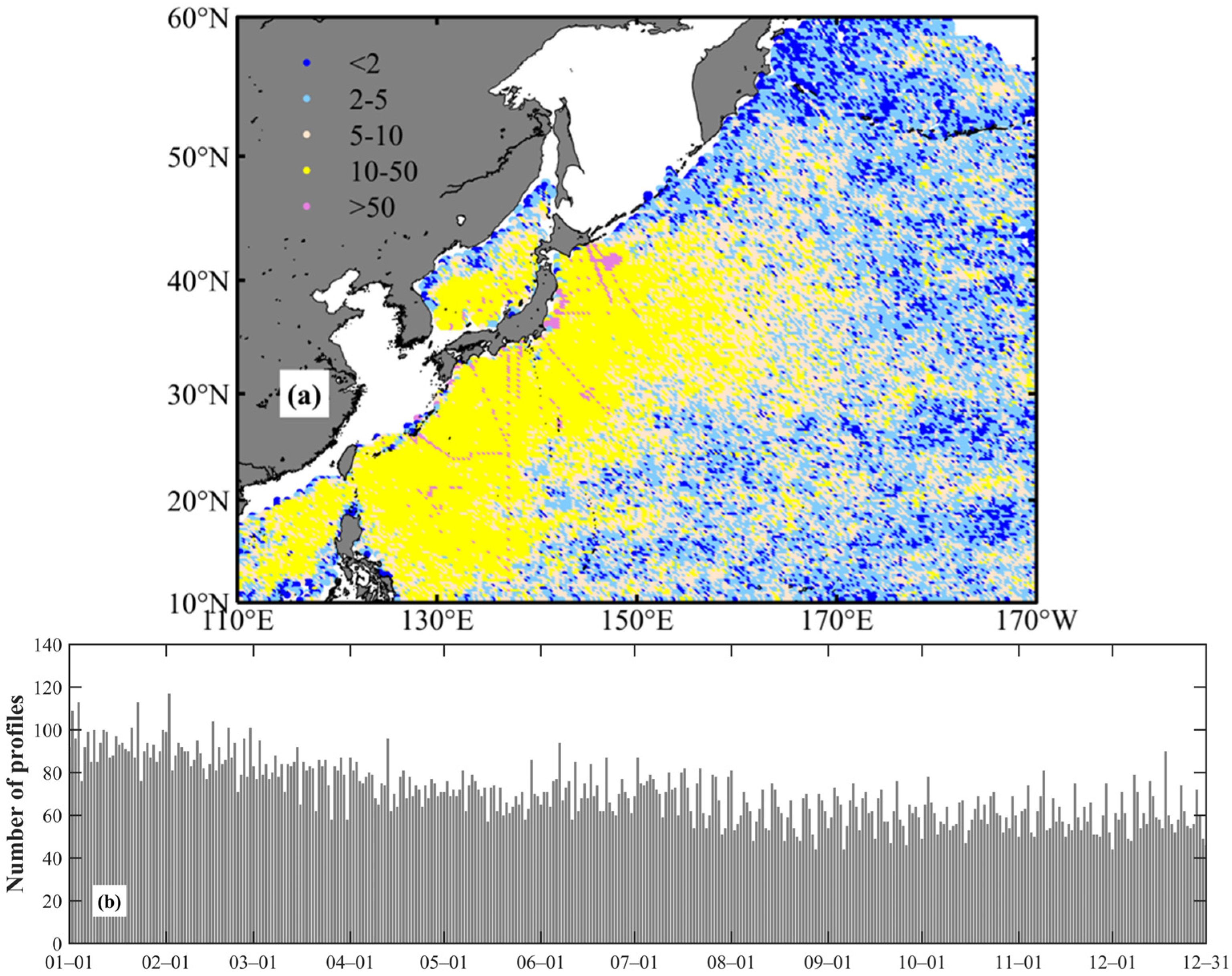
Figure 1. Number of observed temperature and salinity profiles within 0.25° × 0.25° grids from 1 January 2004 to 31 December 2024 (a) and the number of daily observation profiles in 2023 (b) over the NWP.
Jmse 14 00976 g001
Figure 2. Construction process of multi-source data integration.
Jmse 14 00976 g002
Figure 3. Time series of RMSEs associated with the temperature (a) and salinity (b) of inverted profiles relative to Argo observations in 2023.
Jmse 14 00976 g003
Figure 4. Scatter density distributions of temperature (a) and salinity (b) from inverted profiles and Argo observations in 2023. The red dotted line is a linear fitting line.
Jmse 14 00976 g004
Figure 5. Locations of comparative profiles (a) and comparison between inverted profiles and Argo observations on 1 October 2023. Green triangles (P1–P10) denote the locations of temperature profiles (b1b10) and salinity profiles (c1c10).
Jmse 14 00976 g005
Figure 6. Variations in RMSEs and correlation coefficients associated with the temperature and salinity of reconstructed results based on the observations with different parameters. (a,c,e) represent the RMSEs of temperature and salinity under different correlation scale constants, relative observation errors, and search radius, respectively. (b,d,f) represent the correlation coefficients of temperature and salinity under different correlation scale constants, relative observation errors, and search radius, respectively.
Jmse 14 00976 g006
Figure 7. RMSE scatter distribution of GDCSMV3 temperature (a) and salinity (b) relative to the Argo and WOD observations.
Jmse 14 00976 g007
Figure 8. Time series of RMSEs for reconstructed results relative to the Argo and WOD observations from 1 January 2023 to 31 December 2023. (a) Time series of mean RMSEs for temperature and salinity in the upper 1000 m, where the blue dotted line and the red dotted line represent the mean value of the RMSEs of temperature and salinity, respectively. (b) Time series of RMSE for temperature at different depths. (c) Time series of RMSE for salinity at different depths.
Jmse 14 00976 g008
Figure 9. Temperature spectrum analysis results of different datasets at 100 m on 1 October 2023. (a1a3) represent the temperature spectrum analysis results of GDCSMV3, GLORYS2V4, and C-GLORSv7 in region A, respectively. (b1b3) represent the temperature spectrum analysis results of GDCSMV3, GLORYS2V4, and C-GLORSv7 in region B, respectively. (c1c3) represent the temperature spectrum analysis results of GDCSMV3, GLORYS2V4, and C-GLORSv7 in region C, respectively. (d) represents the analysis area division.
Jmse 14 00976 g009
Figure 10. Salinity spectrum analysis results of different datasets at 100 m on 1 October 2023. (a1a3) represent the salinity spectrum analysis results of GDCSMV3, GLORYS2V4, and C-GLORSv7 in region A, respectively. (b1b3) represent the salinity spectrum analysis results of GDCSMV3, GLORYS2V4, and C-GLORSv7 in region B, respectively. (c1c3) represent the salinity spectrum analysis results of GDCSMV3, GLORYS2V4, and C-GLORSv7 in region C, respectively. (d) represents the analysis area division.
Jmse 14 00976 g010
Figure 11. Temperature differences for different datasets relative to XBT on 13 October 2023. (a) XBT station. (b) XBT zonal temperature section. (ce) represent the temperature difference sections of GDCSMV3, GLORYS2V4, and C-GLORSv7 relative to XBT, respectively. The green triangles in (a) represent the locations of XBT stations and the green triangles in (be) represent the longitude of XBT.
Jmse 14 00976 g011
Figure 12. Time series of temperature and salinity from different datasets at depths of 0–1000 m at the site (38° N, 153° E). (a,c,e) are the temperature time series of GDCSMV3, GLORY2V4, and C-GLORSv7, respectively, and (b,d,f) are the corresponding salinity time series.
Jmse 14 00976 g012
Figure 13. The currents of GDCSMV3 at 100 m and the Kuroshio paths extracted based on the currents. (ad) are the identification results of 5 February, April, June, and August 2023, respectively, where the black line represents the identified Kuroshio path.
Jmse 14 00976 g013
Figure 14. The mesoscale eddy identification results of the 100 m GDCSMV3 currents on 1 October 2023, and the temperature and salinity sections of a typical eddy. (a) The distribution of the current and eddy identification results. The blue circle and the red circle represent the cyclonic and anticyclonic eddy boundaries, respectively, and the blue dot and the red dot represent the eddy center. (b) The current distribution of typical eddy. (c) The distribution of eddy numbers for GDCSMV3, GLORY2V4, and C-GLORSv7 within different eddy radius intervals (0.1° intervals). (d,f) are the zonal sections of the cyclone and anticyclone eddy centers, respectively, and (h,j) are the corresponding salinity zonal sections. (e,g) are the meridional sections of the eddy center of cyclone and anticyclone, respectively. (i,k) are the corresponding salinity meridional sections, and the purple dotted lines of (dk) represent the position of the eddy center.
Jmse 14 00976 g014
Disclaimer/Publisher’s Note: The statements, opinions and data contained in all publications are solely those of the individual author(s) and contributor(s) and not of MDPI and/or the editor(s). MDPI and/or the editor(s) disclaim responsibility for any injury to people or property resulting from any ideas, methods, instructions or products referred to in the content.