Multi-Strategy Cooperative Optimization for Coupling Interference Mitigation in the Active Control Filter of a Ship Hydraulic System

Abstract

To address the performance degradation caused by coupling interference between control and identification filters in the active control of ship hydraulic systems, a multi-strategy collaborative optimization algorithm based on “Signal–Amplitude–Time” is proposed. The method constructs a variable-power white-noise module based on power factors to reduce auxiliary noise interference. It employs an improved variable-step-size LMS algorithm to achieve fast and high-precision online identification of the secondary path. Furthermore, an adaptive prediction error filter is introduced to decouple the control and identification processes, effectively resolving the conflict between convergence speed and steady-state precision. Simulation and experimental results demonstrate that the proposed optimization algorithm exhibits superior robustness and adaptive capability under various operating conditions. It can track complex load fluctuations in real time and achieve a line-spectrum pulsation attenuation of more than 90%. This multi-strategy collaborative scheme significantly enhances the pulsation suppression accuracy and dynamic response capability of ship hydraulic systems, providing an efficient and reliable technical approach for the acoustic stealth control of naval ship hydraulic systems.

1. Introduction

Ships serve as the core equipment for surface and underwater operations, and their stealth performance directly determines survivability and breakthrough efficiency on the battlefield. Reducing radiated noise and minimizing detection distance are key to seizing the initiative in naval warfare and can even play a decisive role in turning the tide of war. Within the complex power architecture of a ship, the hydraulic system acts as the central power source for propulsion, steering, and various actuators; thus, its operational stability is of paramount importance. However, due to pump source characteristics and load fluctuations, hydraulic systems inevitably generate fluid pulsations [1]. These pulsations are not only a primary source of pipeline acoustic radiation but also excite intense vibrations in mechanical structures, thereby threatening the service performance and reliability of precision components [2,3,4]. Therefore, researching hydraulic system pulsation suppression is an urgent requirement and core task for developing “quiet” ships and achieving breakthroughs in acoustic stealth.

Currently, the control of hydraulic system pressure pulsations primarily relies on passive suppression methods. This involves installing pulsation attenuators and accumulators to absorb pressure pulsations or using vibration isolation devices such as isolators and pipe clamps to inhibit pulsation propagation. These methods often feature fixed structural parameters or require manual adjustment, lack adaptive capabilities, and exhibit suboptimal attenuation effects for low-frequency pulsations [5]. Therefore, for ship hydraulic systems with complex working environments and variable operating parameters over time, active control with parameter adaptability, strong real-time performance, and significant low-frequency suppression capability has become an effective means of controlling pressure pulsations.

Active control of hydraulic pressure pulsations originated from active noise control (ANC), which can be traced back to 1933 when German physicist Lueg [6] proposed noise cancellation by superimposing a secondary source onto the primary source based on Huygens’ principle. Similar to acoustic noise reduction, active control in hydraulic systems generates a secondary pulsation wave with the same amplitude and frequency as the original pulsation but with a 180° anti-phase. This secondary wave superimposes with the primary wave to cancel peaks and fill troughs, thereby suppressing pressure pulsations. The Filtered-x Least Mean Square (FxLMS) algorithm is the most commonly used algorithm in active control. This algorithm introduced the concept of the secondary path, which represents the transfer function between the control signal and the error signal. Since the secondary path exerts a filtering effect on the output control signal, the core of active control algorithms lies in the estimation of the secondary path. Failing to accurately model the secondary path can severely degrade the performance of the active controller or even cause system divergence.

Offline identification of secondary paths is mostly applied to stable systems [7,8,9]; however, in practical control systems, various degrees of interference are often present. For instance, fluid in hydraulic systems is influenced by factors such as valve opening/closing and irregular piping, which lead to nonlinear and time-varying characteristics in the secondary path. Therefore, to ensure algorithmic stability and achieve effective pulsation control, online modeling methods are generally adopted to perform real-time modeling of the secondary path while the control system is operating. Eriksson [10] first proposed an online modeling method that introduced random white noise as an auxiliary signal. Nevertheless, the introduction of this additional signal causes mutual interference between the identification and control processes, severely degrading the performance of the control system. To resolve this mutual interference, Zhang et al. [11] proposed a secondary path modeling method involving the cross-updating of an identification filter, a control filter, and a third adaptive filter. However, the inclusion of a third filter significantly increases the design and computational complexity of the control system. From the algorithms of Bao [12] and Zhang to that of Yang [13], the underlying approach has been to improve control performance by increasing the number of adaptive filters. While this indeed eliminates the mutual influence between identification and control, the drawbacks are prominent: it increases the burden on the control system and elevates algorithmic complexity.

Akhtar et al. [14] improved upon Eriksson’s method by applying a variable-step-size LMS algorithm to the identification filter, which accelerated identification convergence; however, the white noise continued to limit control performance. To address the deficiencies of Akhtar’s method, A. Carini [15] applied an optimal variable-step-size method to update the secondary modeling filter. Yet, due to the introduction of the MFxLMS algorithm structure, its computational complexity even exceeded that of Zhang’s algorithm. Chen et al. [16] proposed an improved variable-step-size LMS (PVSS-LMS) algorithm for secondary path modeling, while allowing the step size of the control filter to adaptively update according to the correlation value of the error signal and the primary noise energy, thereby enhancing convergence speed while reducing the impact of noise signals on the control process. Zhang et al. [17] introduced the arctangent function into the VSS-FxLMS algorithm for duct noise suppression, demonstrating favorable application potential. In 2023, Li and Zhao [18] proposed a parameter-free VSSLMS algorithm based on the hyperbolic tangent function, achieving step-size updates through error signal mean analysis to improve noise immunity, although its robustness in complex environments requires further enhancement. Jiang et al. [19] proposed a VSS-FxLMS algorithm based on the hyperbolic secant function, which was successfully applied to blade vibration control with significant results.

Addressing the shortcomings of Eriksson’s method, Dou [20] introduced an adaptive error predictor for secondary path modeling, overcoming the influence of narrowband interference during the modeling process and improving modeling accuracy, though the impact of noise on the control filter weight coefficients was not considered. Pu [21] proposed a method for dynamically adjusting the random white-noise power, reducing the influence of auxiliary white noise on the control process. Davari et al. [22] not only introduced variable-power white noise but also added appropriate dynamic adjustment coefficients to the step sizes of both the control and identification filters, achieving higher performance. Zheng et al. [23] proposed an adaptive algorithm for real-time model identification, which combines the recursive prediction error method with traditional filtered adaptive control algorithms to estimate the finite impulse response (FIR) model of the control channel in real time. Yu et al. [24] performed online modeling of the secondary path via additive white noise and introduced a power factor to adjust the active control iteration step size and white-noise power within a set range. Wu et al. [25] utilized an adaptive prediction error filter to achieve decoupling between vibration cancellation and the secondary path; by decoupling the control and identification modules at the signal level, optimization and identification proceed simultaneously, eliminating the mutual influence between the two processes.

Based on previous research, this paper optimizes and proposes an active control algorithm suitable for ship hydraulic systems. To solve the coupling interference between the control and identification filters, a variable-power white-noise module based on a power factor is constructed, an improved variable-step-size LMS algorithm is proposed for online secondary path identification [26], and an adaptive prediction error filter is used to decouple the identification and control processes.

2. Problem Statement

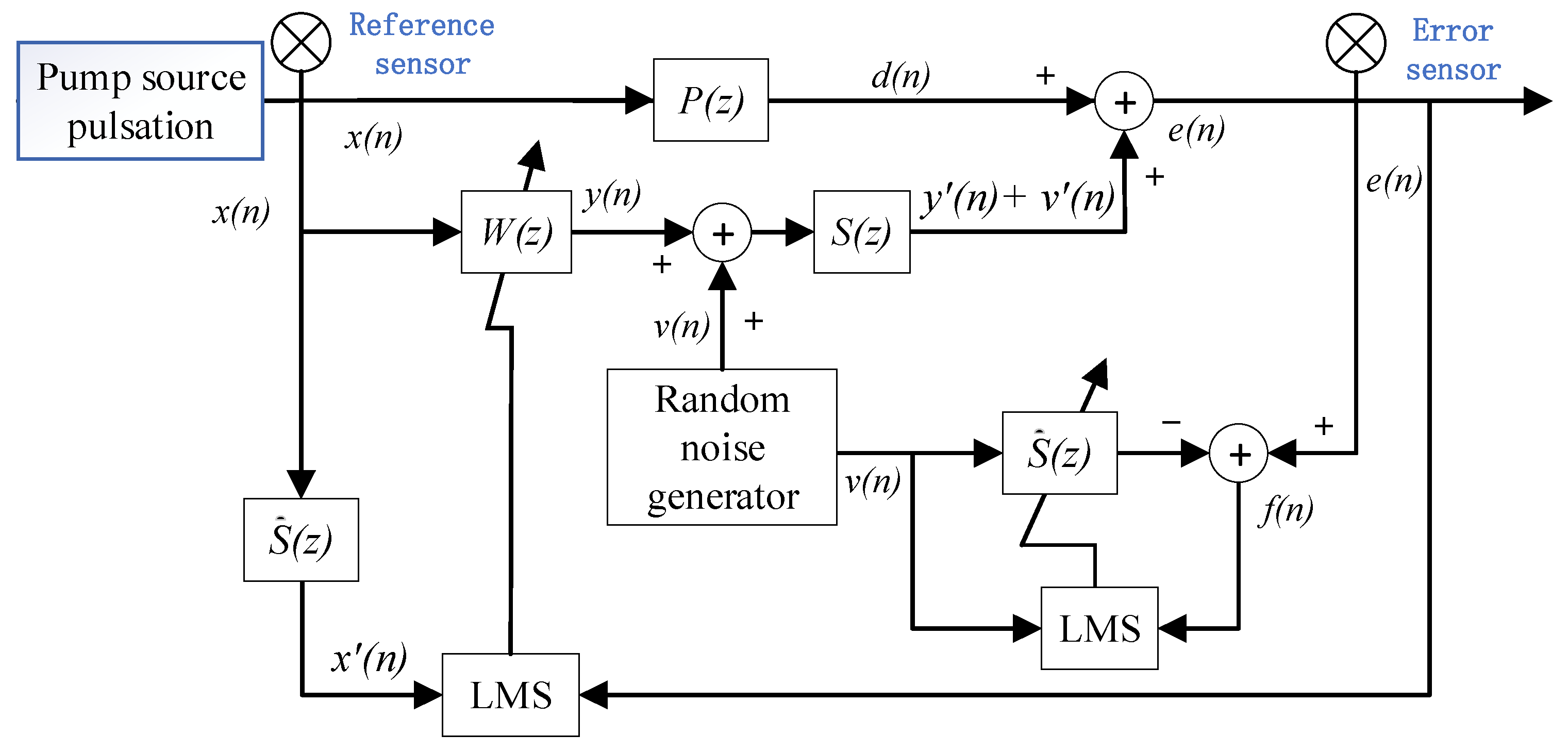
Based on the aforementioned analysis, current research on active control primarily focuses on mitigating the mutual interference between the modeling filter and the control filter. This issue originates from the online secondary path modeling method proposed by Eriksson, which introduces random white noise as an auxiliary signal. The block diagram of Eriksson’s online secondary path identification system is shown in Figure 1. In the figure, $x(n)$ represents the reference signal collected by the reference sensor, $e(n)$ represents the error signal measured by the error sensor, $y(n)$ represents the output signal of the filter, $P(z)$ indicates the primary channel, $S(z)$ represents the secondary channel, and $S^{\prime }(z)$ is the estimation of the secondary channel. In this system, the discrete time-domain signal is represented by the index n (for example, $x(n)$), while the transfer function of the system is expressed in the z-transform domain (for example, $P(z)$), and this rule will be followed throughout the text.

Based on the standard FxLMS algorithm, Eriksson’s method adds a secondary path modeling module, which achieves real-time identification of the secondary path by injecting an auxiliary noise signal during system operation. The system consists of two parallel adaptive filters: the control filter $W(z)$ used to generate the control signal for noise cancellation, and the modeling filter $\widehat{S}(z)$ used to estimate the characteristics of the secondary path. To achieve online identification of the secondary path, an independent white-noise signal $v(n)$ is introduced as an excitation signal. In this system, the signal received by the error sensor is:

$$e(n)=d(n)+y^{\prime }(n)+v^{\prime }(n)$$

(1)

where $y^{\prime }(n)=-y(n)\ast s(n)$ represents the output of the control signal after passing through the secondary path, and $v^{\prime }(n)=v(n)\ast s(n)$ denotes the output of the training signal after passing through the secondary path. The LMS algorithm is employed for secondary path modeling. The output of the modeling filter is defined as:

$${\widehat{v}}^{\prime }(n)={\widehat{s}}^T(n)v(n)$$

(2)

where $\widehat{s}(n)$ is the weight vector of the modeling filter, and $v(n)={[v(n),v(n-1),\dots ,v(n-M+1)]}^T$ is the training signal vector.

The core problem of Eriksson’s method lies in the composition of the modeling error signal $f(n)$. Expanding it:

$$f(n)=[d(n)+y^{\prime }(n)]+[v^{\prime }(n)-{\widehat{v}}^{\prime }(n)]$$

(3)

The signal consists of two parts: $[v^{\prime }(n)-{\widehat{v}}^{\prime }(n)]$ is the true modeling error, which reflects the difference between the model and the actual secondary path; $[d(n)+y^{\prime }(n)]$ is the interference term, namely the residual noise from the control process.

Theoretically, the LMS algorithm should update the weight coefficients based on the true modeling error. However, in Eriksson’s method, the algorithm actually utilizes the interference-contaminated signal $f(n)$. This contamination leads to a bias in the gradient estimation, which severely degrades the convergence performance of the modeling process.

The impact of the interference term $[d(n)+y^{\prime }(n)]$ on the modeling process is also reflected in the perturbation of the gradient. The instantaneous gradient estimate of the modeling filter is:

$$\begin{array}{ll}{\nabla }_{s}J(n)& =-2v(n)f(n)\\ & =-2v(n)[d(n)+y^{\prime }(n)]-2v(n)[v^{\prime }(n)-{\widehat{v}}^{\prime }(n)]\end{array}$$

(4)

The first term, $-2v(n)[d(n)+y^{\prime }(n)]$, represents the gradient perturbation caused by interference. Since $v(n)$ is statistically independent of $[d(n)+y^{\prime }(n)]$, the expectation of this perturbation term is zero, but its variance is non-zero. This causes random fluctuations in the weight coefficient update path, thereby reducing the convergence speed.

According to the stability constraints of the algorithm, and considering the impact of interference, the step-size selection for the modeling filter must satisfy more stringent stability conditions:

$$0<{\mu }_s<{\displaystyle \frac{2}{{\lambda }_{\max }({\mathbf{R}}_v)+\alpha P^{\prime }/{\sigma }_v^2}}$$

(5)

where ${\mathbf{R}}_v$ is the autocorrelation matrix of the training signal; ${\sigma }_v^2$ is the power of the random white noise; $P^{\prime }=E[{\left|d(n)+y^{\prime }(n)\right|}^2]$ is the interference power. It can be observed that the larger the interference power, the smaller the maximum allowable step size.

For Eriksson’s algorithm, not only does the control filter exert an interference effect on the modeling filter, but the modeling filter also significantly interferes with the control filter. Expanding Equation (3) yields:

$$f(n)=x(n)\ast p(n)-y(n)\ast s(n)+v(n)\ast s(n)-v(n)\ast \widehat{s}(n)$$

(6)

where $p(n)$ is the finite impulse response of the primary path. Taking the Z-transform of the above equation gives:

$$\begin{array}{ll}F(z)& =X(z)P(z)-X(z)W(z)S(z)\\ & +V(z)S(z)-V(z)\widehat{S}(z)\end{array}$$

(7)

During system operation, the controller can theoretically output the optimal control signal only after the precise modeling of the secondary path is completed. Therefore, as the control filter continues to converge, in the ideal case where $n\to \infty$, $f(n)\to 0$. At this point, the weights of the control filter converge to the optimal value:

$$W^{\prime }(z)={\displaystyle \frac{P(z)}{S(z)}}+\left({\displaystyle \frac{S(z)-\widehat{S}(z)}{S(z)}}\right){\displaystyle \frac{V(z)}{X(z)}}$$

(8)

As shown in Equation (8), the control filter $W(z)$ converges to its optimal value $P(z)/S(z)$ if and only if $\widehat{S}(z)=S(z)$. Thus, the modeling filter directly influences the convergence of the control filter.

Through this analysis, it is evident that although the Eriksson method achieves online modeling of the secondary path, the coupling interference between the control and modeling processes severely limits system performance:

(1)

The error signal is contaminated by the excitation white-noise signal, leading to inaccurate gradient estimation and slow convergence;

(2)

The presence of interference forces the use of conservative step-size settings, further restricting the convergence speed;

(3)

The mutual influence between the control and modeling filters creates a vicious cycle.

3. Proposed Algorithm

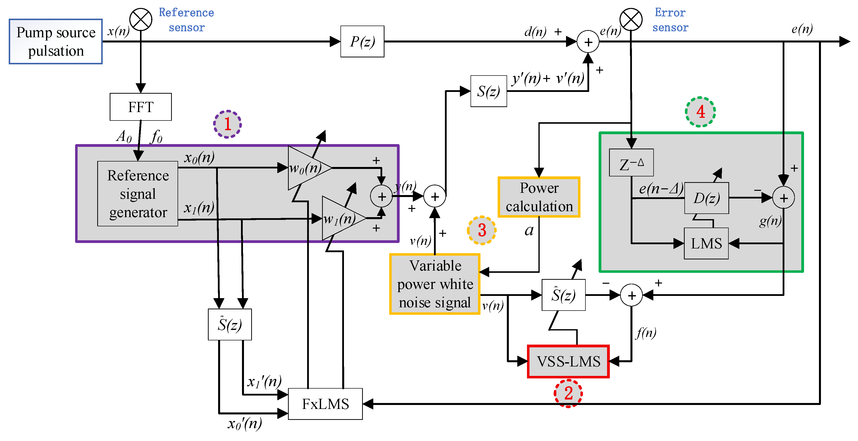
Based on the FxLMS algorithm, this paper proposes an active control algorithm as shown in Figure 2. The architecture of the algorithm primarily consists of four modules: (1) an adaptive notch filter, (2) variable-step-size online identification of the secondary path, (3) variable-power white noise, and (4) a prediction error filter.

3.1. Adaptive Trap Filter

In 1995, Kuo et al. [27] proposed an adaptive notch algorithm specifically for single-frequency noise control. Based on the LMS or FxLMS algorithms, the adaptive notch algorithm adjusts the input signal. The input signal used by the algorithm is also referred to as the “reference signal,” which is a sinusoidal signal of a specific frequency. This implies that the input signal is free from interference and uncertainty, making it easier for the algorithm to converge. In hydraulic systems, pressure pulsations are often concentrated at several specific frequency points; therefore, the notch algorithm is highly suitable for application in the active control of hydraulic systems.

In hydraulic systems, the original pressure pulsation signal $x(n)$ is first collected over a certain period using a pressure sensor. A Fast Fourier Transform (FFT) is performed on this signal to obtain the primary pulsation line-spectrum frequencies $f_0$ and their corresponding amplitudes $A_0$ of the initial pressure pulsation signal. By inputting the target pulsation frequency $f_0$ and amplitude $A_0$ into the adaptive notch filter, a reference signal composed of two mutually orthogonal signals can be constructed.

$$x_{m,0}\left(n\right)=A_{m0}\sin \left(2\pi f_{m0}n\right),m=1,2,\dots ,M$$

(9)

$$x_{m,1}\left(n\right)=A_{m0}\cos \left(2\pi f_{m0}n\right),m=1,2,\dots ,M$$

(10)

Here, m denotes the number of control spectral lines, $f_{m0}$ represents the frequency of the m-th spectral line to be suppressed from the original pulsation obtained via FFT, $A_{m0}$ denotes its corresponding spectral amplitude, and n signifies the n-th time point.

3.2. Variable-Step-Size Online Identification of Secondary Channels

The convergence speed is a key metric for evaluating whether active control can effectively suppress pressure pulsations in naval hydraulic systems. Taking the naval steering gear as an example, the steering actions are rapid and frequent, with a single steering duration lasting only a few to a dozen seconds. This requires the control algorithm to achieve convergence within an extremely short time to ensure effective suppression of pressure pulsations. The convergence speed directly depends on the selection of the algorithm’s step-size parameters. However, the traditional fixed step-size LMS algorithm faces an inherent trade-off between convergence speed and steady-state error: on one hand, a larger step size can significantly accelerate the initial convergence process but often leads to increased steady-state error and the risk of divergence; on the other hand, a smaller step size helps effectively reduce the steady-state error but significantly slows down the convergence speed, making it difficult to adapt to the fast changing characteristics of pressure pulsations in hydraulic systems.

To resolve this contradiction, variable-step-size LMS algorithms have emerged. These algorithms dynamically adjust the step-size parameters based on the error signal or system state, employing a larger step size in the initial stage of convergence to accelerate the iterative process and gradually switching to a smaller step size after entering the stable stage. This effectively reduces the steady-state error and enhances overall adaptability.

To achieve both fast convergence speed and superior steady-state error performance, this paper proposes a dual-nonlinear function collaborative-coupled nonlinear variable step-size FxLMS algorithm (DCNVSS-FxLMS). The corresponding step-size formula is defined as:

$$\mu (n)={\mu }_{\max }\cdot {\displaystyle \frac{e^2(n)}{e^2(n)+{\beta }^2}}\cdot \left(1-e^{-\alpha \left|e(n)\right|}\right)$$

(11)

where ${\mu }_{\max }$, $\alpha$, and $\beta$ are three defined parameters. By adjusting the values of these parameters, the shape characteristics of the step-size function curve can be precisely controlled. This step-size function ingeniously combines two nonlinear mechanisms: a rational fraction term and an exponential term, in order to achieve adaptive step-size adjustment. Monotonicity: The derivative of the step-size function is always greater than zero, verifying that the step-size function is monotonically increasing with respect to the absolute value of the error. This characteristic ensures the ideal regulation mechanism: “larger error, larger step size to accelerate convergence; smaller error, smaller step size to improve precision.” Boundedness: When $\left|e\left(n\right)\right|\to 0$, $\mu \left(n\right)\to 0$; when $\left|e\left(n\right)\right|\to \infty$, $\mu \left(n\right)\to {\mu }_{\max }$. Combined with the monotonicity of the step-size function, it ensures that $0\le \mu \left(n\right)\le {\mu }_{\max }$ remains within a stable range, preventing the algorithm from exceeding the stability convergence boundaries under any circumstances.

From a functional design perspective, the rational fraction term provides a smooth step-size transition during error changes, effectively avoiding abrupt step-size mutations and thereby enhancing the stability of the algorithm. The exponential term changes relatively steadily within the small error range, providing fine-grained step-size control. Through reasonable parameter configuration, the organic combination of the rational fraction and the exponential function allows the step-size function to maintain a larger step size in the initial stage of convergence to accelerate speed, while maintaining a very small step size in the small error region to ensure low steady-state error.

3.3. Prediction Error Filter

In the online identification of the secondary path, the excitation signal is ideally an independent white-noise signal $v(n)$. However, as indicated by Equation (3), the signal $f(n)$ input to the modeling filter contains the interference term $[d(n)+y^{\prime }(n)]$. Compared to the white noise response, the amplitude of the interference signal is quite large, which often leads to inaccurate secondary path identification or even divergence of the control algorithm. To weaken the influence of the control process on the identification process and provide a more accurate error signal for the modeling filter weight update, an online secondary path identification method using a prediction error filter for decoupling is employed.

Let $v_{\mathrm{disturb} }(n)=d(n)+s(n)*y(n)$, then the error signal $e(n)$ is given by:

$$e(n)=v_{\mathrm{disturb} }\left(n\right)+s\left(n\right)*v\left(n\right)$$

(12)

Due to the existence of line-spectrum pulsations in the hydraulic system, the primary path signal $d(n)$ contains periodic narrowband components; thus, $v_{\mathrm{disturb} }(n)$ also contains the same periodic narrowband components. In the adaptive prediction error filter section, an adaptive filter and a delay unit are constructed. The objective is to make the broadband signal components excited by white noise uncorrelated with $e(n)$, while the interference signal components $v_{\mathrm{disturb} }(n)$ remain correlated with $e(n)$, thereby utilizing the adaptive prediction error filter to filter out the interference signal components $v_{\mathrm{disturb} }(n)$.

Assuming the secondary path $S(z)$ can be modeled by an M-order finite impulse response (FIR) filter, the error signal obtained by the error sensor can be expressed as:

$$e(n)=v_{\mathrm{disturb} }\left(n\right)+{\displaystyle \sum _{j=0}^{M_s-1}}{s}_j\left(n\right)v\left(n-j\right)$$

(13)

where $s(n)$ is the j-th impulse response of the secondary path $S(z)$ at time n, and $M_s$ is the order of the identification filter.

As shown in Figure 2, the reference error signal $g(n)$ input to the identification filter at this time is:

$$g\left(n\right)=e(n)-e\left(n-\Delta \right)*w_{\mathrm{d} }\left(n\right)$$

(14)

where Δ is the delay of the prediction error filter, and $w_{\mathrm{d} }\left(n\right)$ is the time impulse response signal of the prediction error filter.

Since the white noise exciting the secondary path is a zero-mean white-noise signal uncorrelated with $v_{\mathrm{disturb} }(n)$, the expectation of the cross-correlation between the input and output of the prediction error filter can be obtained as:

$$\begin{array}{l}E\left(e\left(n\right)e\left(n-\Delta \right)\right)=E\left[v_{\mathrm{disturb} }\left(n\right)v_{\mathrm{disturb} }\left(n-\Delta \right)\right]\\ +{\displaystyle \sum _{j=0}^{M_s-1}}{s}_j\left(n\right){\displaystyle \sum _{i=0}^{M_s-1}}{s}_i\left(n\right)\left\{E\left[v\left(n-j\right)v\left(n-i-\Delta \right)\right]\right\}\end{array}$$

(15)

In the equation, the first term $E[v_{\mathrm{disturb} }\left(n\right)v_{\mathrm{disturb} }\left(n-\Delta \right)]$ is related to the interference term $v_{\mathrm{disturb} }(n)$, and the second term is related to the white-noise excitation $v(n)$. Therefore, the parts related to the interference term can be filtered out by selecting an appropriate delay Δ. When the delay satisfies:

$$\Delta \ge M_s$$

(16)

Then:

$$E\left[v\left(n-j\right)v\left(n-i-\Delta \right)\right]=0, 0\le i,j\le M_s$$

(17)

That is, when $M_s\le \Delta$, the error signal $e(n)$ is uncorrelated with the white-noise excitation signal $v(n)$, and is only correlated with the interference term $v_{\mathrm{disturb} }(n)$. At this point, the prediction error filter cannot predict the variations in $e(n)$ related to $v(n)$, and the signal $v_{\mathrm{disturb} }(n)$ is removed by the prediction error filter after the selected delay Δ.

The update formula for the weights $w_d(n)$ of the prediction error filter $D(z)$ is expressed as follows:

$$w_d\left(n+1\right)=w_d\left(n\right)+{\mu }_{d}e\left(n-\Delta \right)g\left(n\right)$$

(18)

When the prediction filter converges, the output of the filter is:

$$\begin{array}{l}g\left(n\right)=v^{\prime }\left(n\right)-v^{\prime }\left(n-\Delta \right)*w_d\left(n\right)\\ \approx v\left(n\right)=v\left(n\right)*s\left(n\right)\end{array}$$

(19)

In the reference signal provided by the prediction error filter $D(z)$ to the modeling filter $S^{\prime }(z)$, the interference term $v_{\mathrm{disturb} }(n)$ has been basically filtered out. Although a new interference term $v^{\prime }\left(n-\Delta \right)*w_d\left(n\right)$ is introduced, which may have a certain impact on the convergence speed of the algorithm, the magnitude of this interference is negligible compared to the original interference. Ultimately, the decoupling of the control process and the modeling process is achieved, weakening the interference of the control process on the modeling process.

3.4. Variable-Power White-Noise Module

In active control systems, the performance of adaptive algorithms depends heavily on the accuracy and robustness of channel identification. Traditional methods often employ fixed-power white noise as the excitation signal for servo valve opening control, thereby generating a corresponding “white-noise pressure” within the system to achieve online identification of the secondary path. However, in practical applications, the system pressure is often in a state of dynamic change. This results in inconsistent pressure fluctuation amplitudes excited by white-noise signals of the same power at different pressure levels: if the power is too low, the identification excitation is insufficient, compromising algorithm convergence and control precision; if the power is too high, excessive vibration may be introduced, weakening the overall suppression effect or even triggering system instability. To address this challenge, an active control algorithm based on variable-power white noise is proposed here, which adaptively adjusts the white-noise power in real time to accommodate system pressure variations, thereby enhancing the adaptability of the identification process and the efficiency of time-domain control.

To realize a variable-power white-noise signal, a power factor $a$ is introduced from a power perspective. The white-noise signal $v(n)$ is regarded as a superposition of a reference white-noise signal $v_0(n)$ and the power factor $a$, and its expression is given by:

$$v(n)=a\cdot v_0(n)$$

(20)

The variation range of the system spectral pulsation is $[p_{min}, p_{max}]$. The power factor is defined to vary linearly with spectral pulsation. Based on empirical and experimental data, the maximum spectral pulsation $P_{\max }$ and minimum spectral pulsation $P_{\min }$ of the hydraulic system correspond to power factors $a_{\max }$ and $a_{\min }$, respectively. From this linear relationship, the expression for the power factor $a$ is derived as:

The variation range of the system line-spectrum pulsation is $[p_{min}, p_{max}]$. The power factor is defined to vary linearly with the line-spectrum pulsation. Based on empirical data and experimental results, the power factors $a_{\max }$ and $a_{\min }$ corresponding to the maximum line-spectrum pulsation $P_{\max }$ and minimum value $P_{\min }$ of the hydraulic system are determined. The expression for the power factor $a$ derived from the linear variation is:

$$a={\displaystyle \frac{a_{\max }-a_{\min }}{P_{\max }-P_{\min }}}\left(P-P_{\max }\right)+a_{\max }$$

(21)

where $P$ is the amplitude of the line-spectrum pulsation obtained by the error sensor.

The variable-power white-noise FxLMS algorithm breaks through the limitations of traditional fixed-power detection signals. By establishing a dynamic mapping relationship between the error signal characteristics and the white-noise power, it achieves intelligent adjustment of the detection signal. The core innovations of the algorithm are:

(1)

Adaptive Power Adjustment Mechanism: The white-noise power is dynamically adjusted according to the real-time amplitude of the error signal, realizing an optimized strategy of “detection on demand.”

(2)

Signal Dynamic Range Normalization: By tracking the changes in the signal’s dynamic range in real time, the algorithm can adaptively adjust the parameters of the power mapping function. This normalization process enables the algorithm to adapt to input signals of different amplitude levels, thereby enhancing its universality and robustness.

4. Simulation Verification

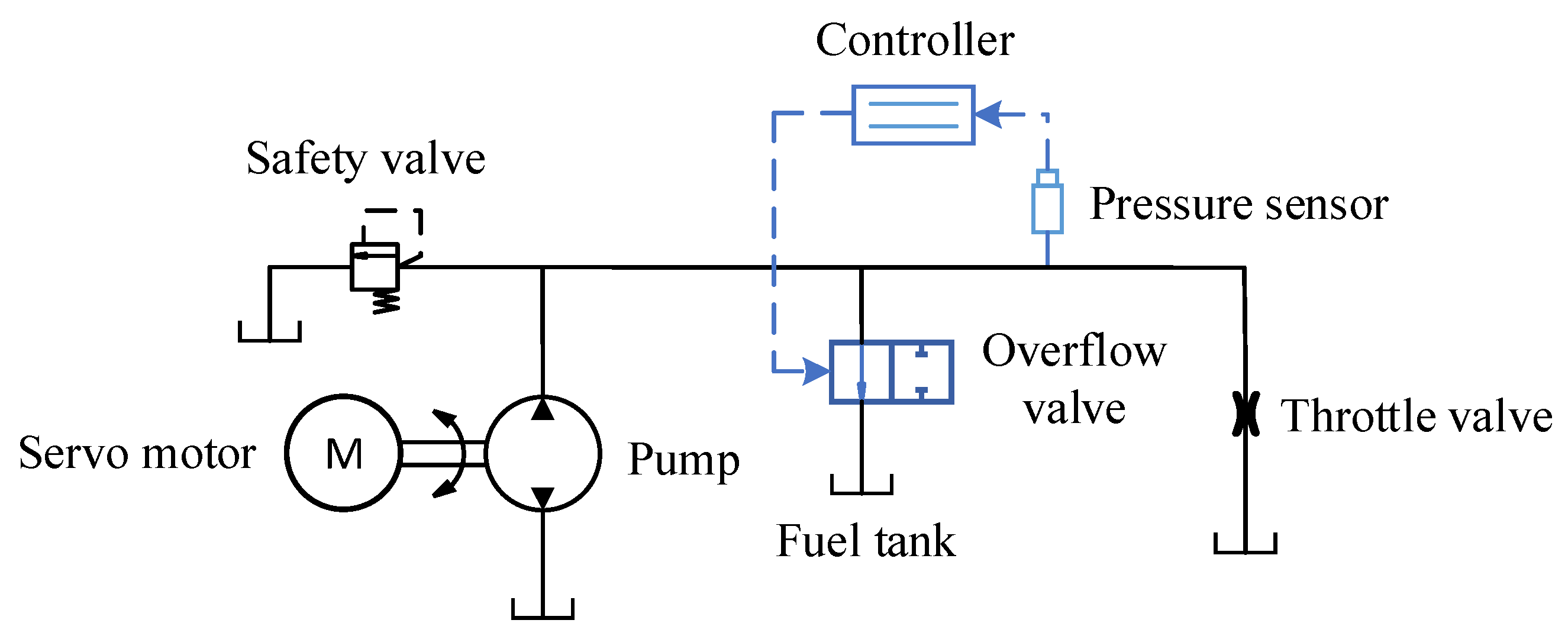
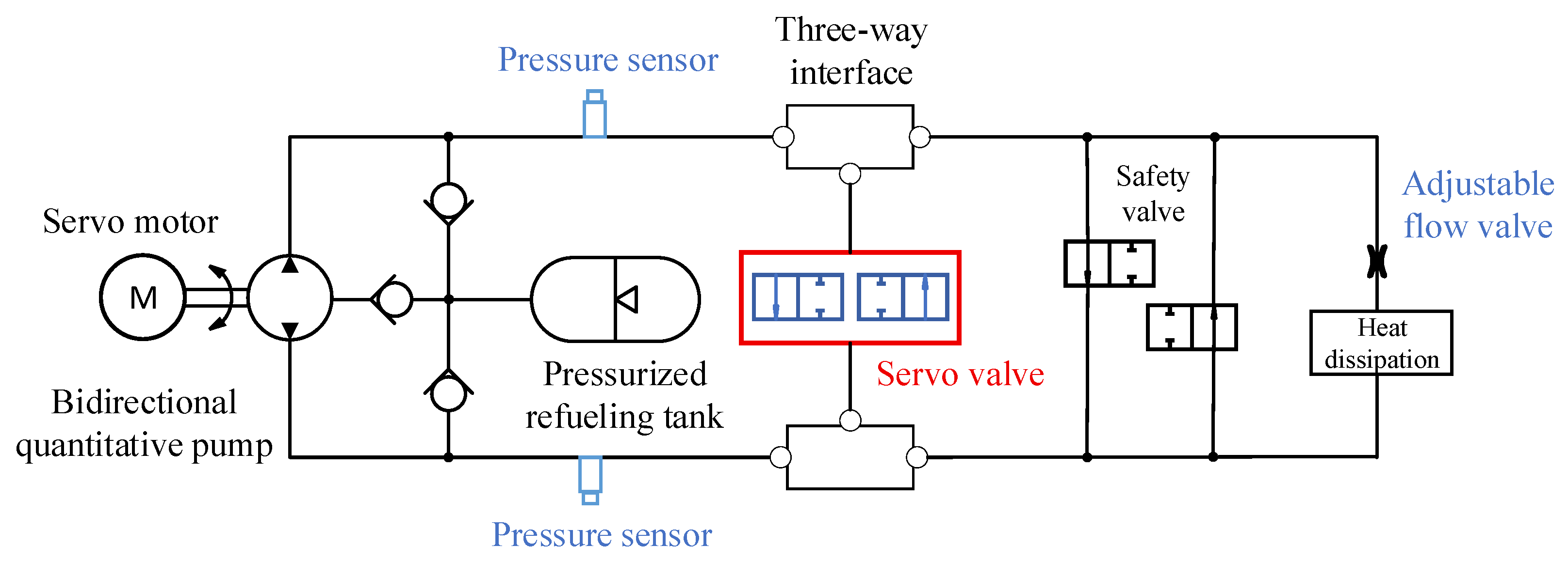
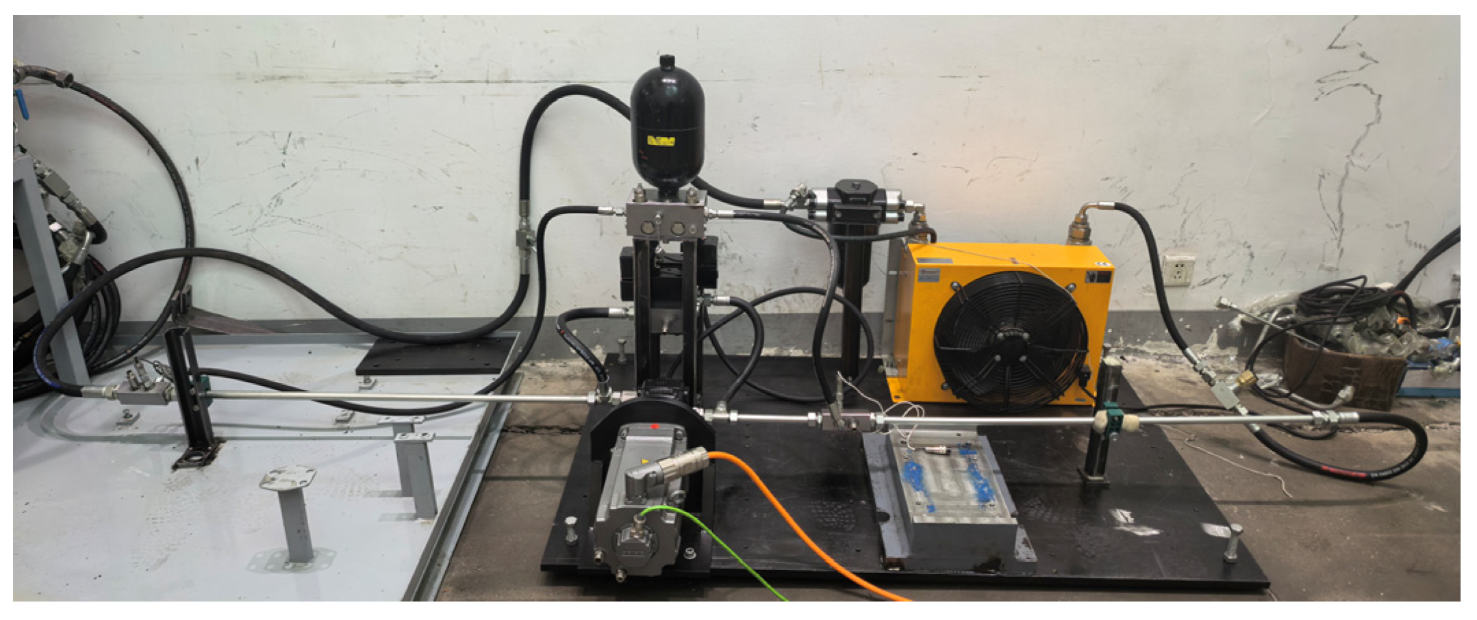
Experiments are conducted using the AMESim-Simulink joint simulation method to evaluate the performance of the active control algorithm. The control scheme follows the spill-type active control principle shown in Figure 3, utilizing the secondary pressure waves generated by the relief valve to cancel out the system’s original pulsations. This scheme is solely aimed at verifying the decoupling mechanism and convergence characteristics of the algorithm, and it eliminates the interference from complex nonlinear physical factors.

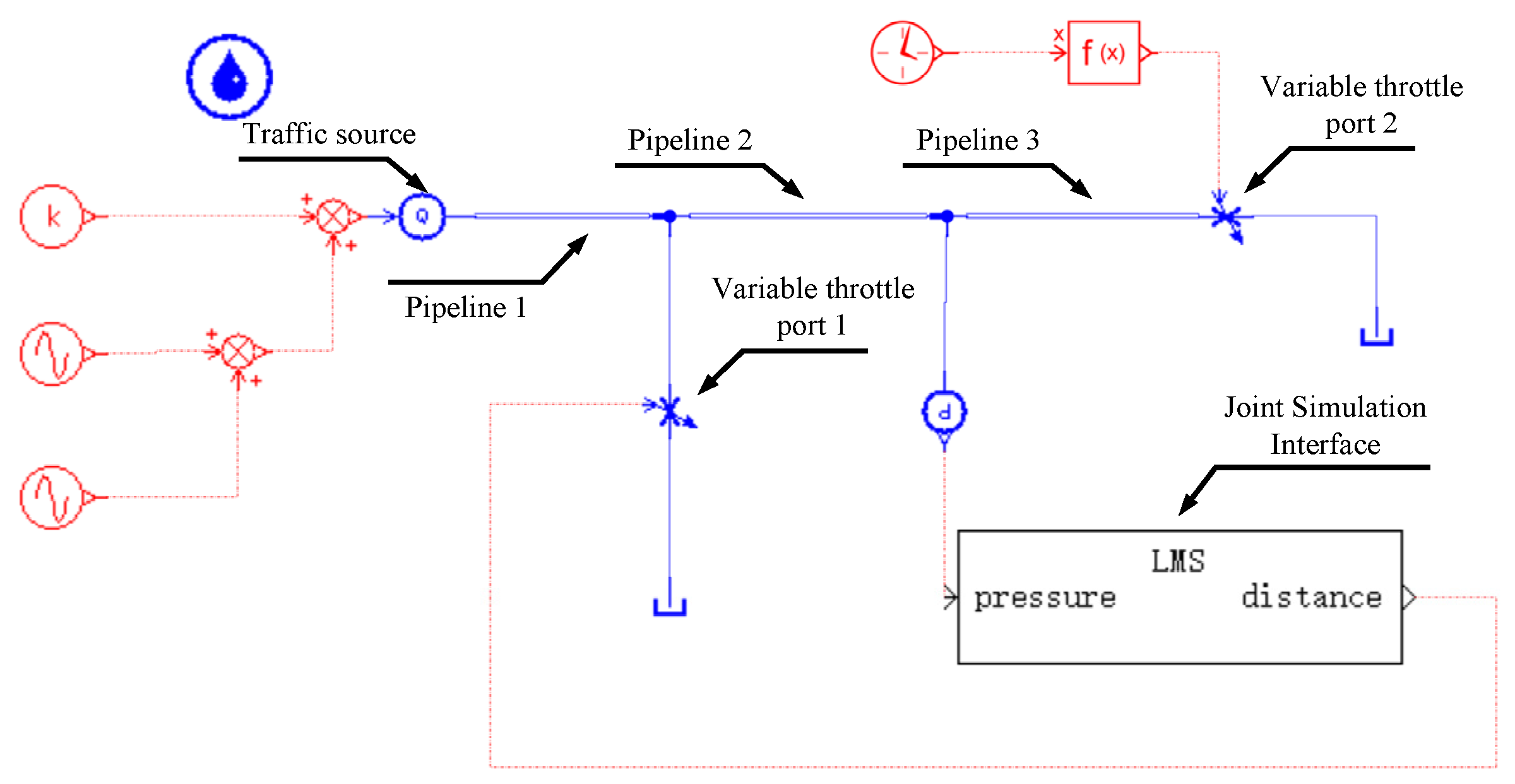
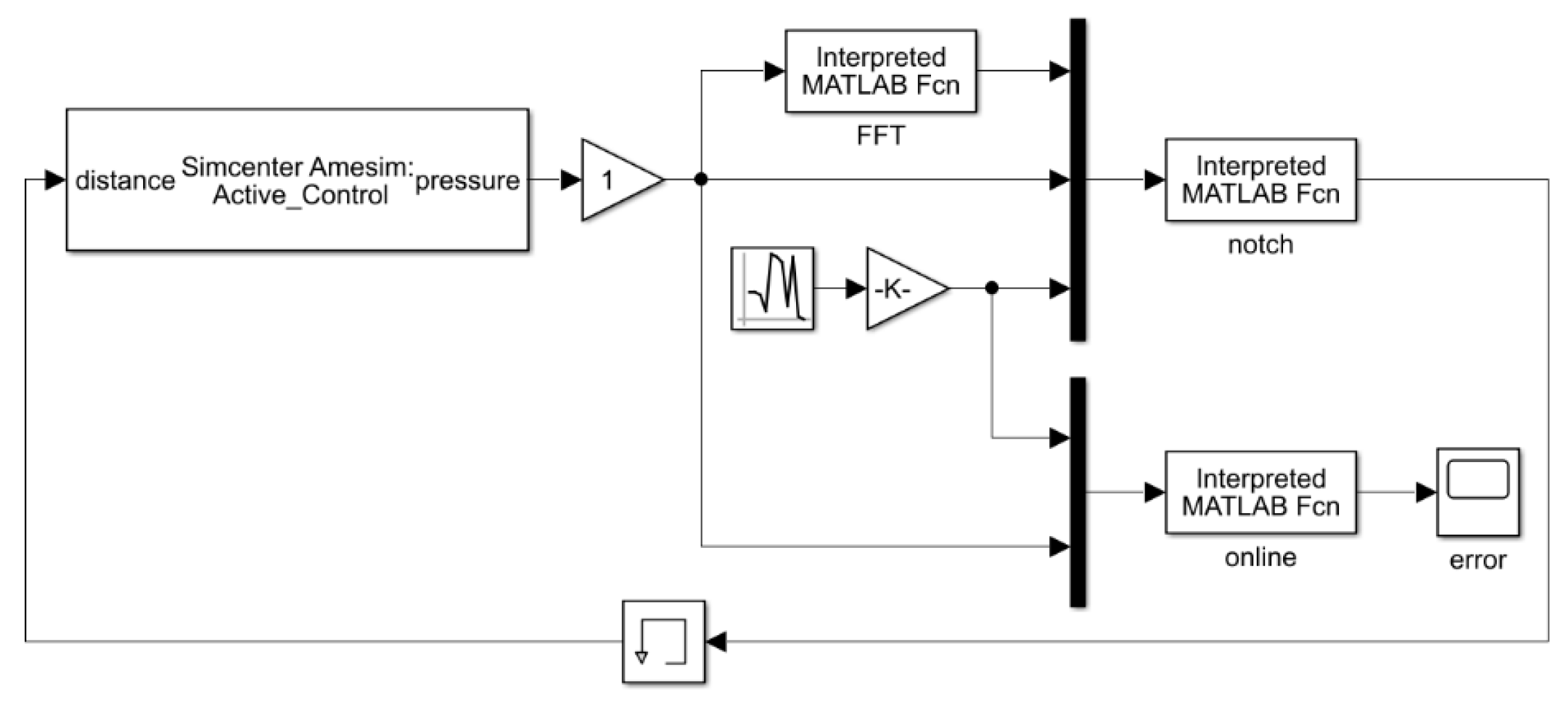
The AMESim side is responsible for the simulation of the hydraulic physical layer, including the flow source, load orifice, and the variable orifice that executes active control. The Simulink side is responsible for the implementation of the algorithmic logic layer. During simulation, real-time signals captured by the pressure sensor are transmitted across platforms to Simulink. After calculation, the control algorithm outputs a control voltage, which acts back on the variable orifice in AMESim. Through this closed-loop regulation, the variable orifice can generate pulsation components with opposite phases, thereby achieving the objective of reducing fluid pulsations. The models in the two simulation environments are shown in Figure 4 and Figure 5, respectively.

In the AMESim model, a flow source (composed of a DC component superimposed with two sinusoidal components) is used to simulate a real “pump source”. “Variable Orifice 1” corresponds to the “relief servo valve used for active control,” with a maximum opening diameter of 3 mm and a control signal range of 0–10. “Variable Orifice 2” serves as the load throttle valve used to simulate variable-load conditions, with a maximum opening diameter of 5 mm and a control signal range of 0–1. The model includes three main pipeline sections, the detailed parameters of which are shown in

Table 1. Parameter settings of the pipeline model.

Pipeline Number	Length (m)	Diameter (mm)	Pipeline Model
Pipeline 1	1	25	Cfd 1d
Pipeline 2	0.2	25	Cfd 1d
Pipeline 3	1	25	Cfd 1d

.

The fluid excitation signal in the pipeline is simulated via a flow generator in the model, and its flow output equation is set as:

$$\begin{array}{l}{Q}_s\left(t\right)=50+6.5\cdot \sin \left(2\pi \cdot {\mathrm{T}}_1\cdot t+23\cdot {\displaystyle \frac{\pi }{180}}\right)\\ +0.5\cdot \sin \left(2\pi \cdot {\mathrm{T}}_2\cdot t-47\cdot {\displaystyle \frac{\pi }{180}}\right)\end{array}$$

(22)

The sampling frequency in the simulation environment is set to 2000 Hz. The fixed step size for the traditional algorithm is set to $\mu =0.0002$, and the parameters for the step-size function are set to ${\mu }_{\max }=0.00219$, $\alpha =8.5$, and $\beta =0.12$. Subsequent simulation experiments will analyze the control effectiveness of the algorithm under two typical working conditions: constant load and time-varying load.

4.1. Constant Load Condition Simulation Analysis

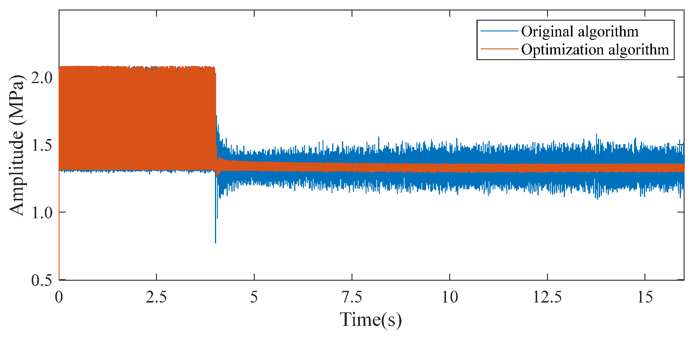
Under constant load conditions, the system’s load orifice opening remains unchanged, aiming to verify the suppression effect and convergence speed of the optimized algorithm in a steady-state operating environment. In the simulation experiment, the average pipeline pressure is 1.7 MPa, and the pulsation signal is composed of a fundamental frequency (40 Hz) and its second harmonic (80 Hz), with a total pulsation amplitude of 0.4 MPa. The system remains uncontrolled for the first 4 s, and active control is activated at t = 4 s.

Figure 6 displays the time-domain response curves of the pipeline pressure pulsations before and after the activation of the active control algorithm under constant load conditions. The orange curve represents the traditional algorithm, while the blue curve represents the optimized algorithm. As shown in the figure, before the control algorithm is engaged, the pressure amplitude alternates between 13 bar and 21 bar, with a peak-to-peak value as high as approximately 8 bar, indicating significant fluid pulsation in the uncontrolled state. When the simulation reaches 4 s and active control is enabled, the traditional algorithm exhibits a certain degree of lag, requiring an adjustment period of approximately 0.4 s to reach a steady state. In contrast, the optimized algorithm achieves convergence in only about 0.13 s, representing a response speed improvement of approximately 67.5%. During the stable control phase, both algorithms effectively suppress pressure pulsations, with specific control metrics detailed in

Table 2. Peak-to-peak pressure values before and after “fixed-power white-noise” control.

Type	Control the Peak-to-Peak Value of the Pre-Pressure (MPa)	Controlled Post-Pressure Peak-to-Peak Value (MPa)	Attenuation Rate
Traditional algorithm	0.7832	0.3291	57.98%
Optimized algorithm	0.7641	0.0465	93.91%

. Upon entering the steady-state control phase, the suppression effect of the optimized algorithm is significantly superior to that of the traditional algorithm. The traditional algorithm reduces the peak-to-peak pressure from 0.7832 MPa to 0.3291 MPa, an attenuation rate of 57.98%. The optimized algorithm significantly improves the control accuracy, reducing the peak-to-peak value from 0.7641 megapascals to 0.0465 megapascals, with an attenuation rate of 93.91%. The pulsation suppression effect has increased by 35.93 percentage points.

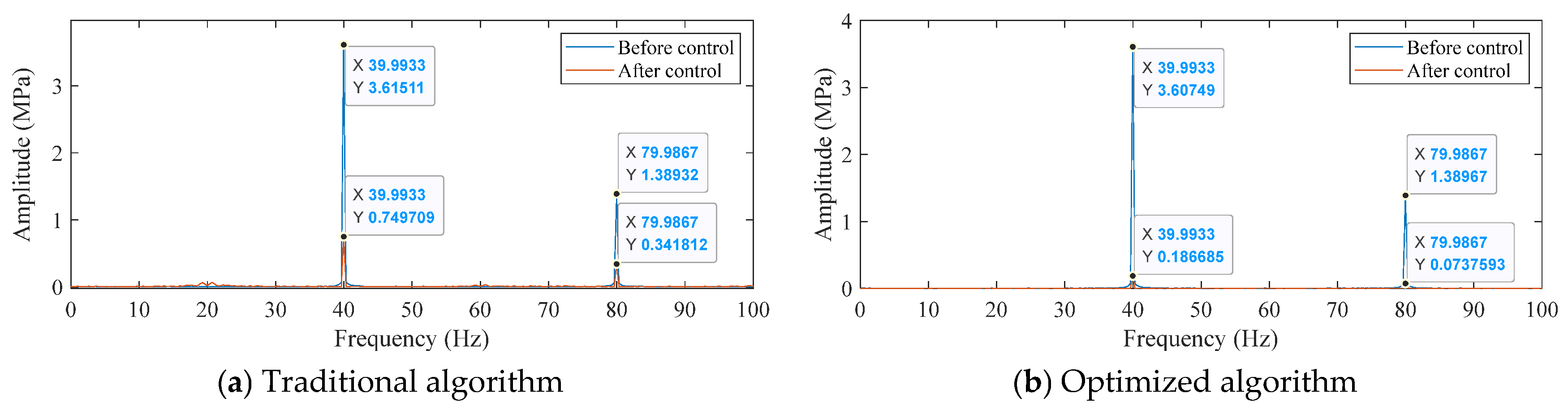
In order to more intuitively evaluate the control strategy’s ability to suppress the pulsating energy in different frequency bands, the pressure signals extracted from the simulation were subjected to fast Fourier transform, and the frequency-domain response characteristics of the system were obtained. Figure 7 presents the comparison chart of the pressure spectrum before and after control for both the traditional algorithm and the optimized algorithm under a constant load condition. Additionally, to quantitatively analyze the control effect,

Table 3. Comparison of pulsation control effects under a constant load environment.

Type	40 Hz			80 Hz
	Amplitude Before Control (MPa)	Amplitude After Control (MPa)	Attenuation Rate	Amplitude Before Control (MPa)	Amplitude After Control (MPa)	Attenuation Rate
Traditional algorithm	3.6151	0.7497	79.26%	1.3893	0.3418	75.40%
Optimized algorithm	3.6075	0.1867	94.83%	1.3897	0.0738	94.69%

has meticulously extracted and compared the amplitudes at the main pulsation frequencies and the corresponding attenuation rates. Compared to the traditional algorithm, the attenuation rates of the pulsations at 40 Hz and 80 Hz for the optimized algorithm have increased by approximately 15 to 19 percentage points, and the attenuation rates have remained above 94% consistently. This clearly demonstrates that in the constant load condition, the optimized algorithm proposed in this paper not only can more accurately track and counteract the main frequency pulsations but also can effectively suppress the harmonic frequencies in a balanced manner, achieving higher steady-state control accuracy and superior comprehensive control performance.

Combining the figures and tables, it is evident that the optimized algorithm not only increases the convergence rate but also achieves a marked improvement in steady-state error, proving its superior capability in fluid pulsation reduction under constant load conditions.

4.2. Time-Varying Load Condition Simulation Analysis

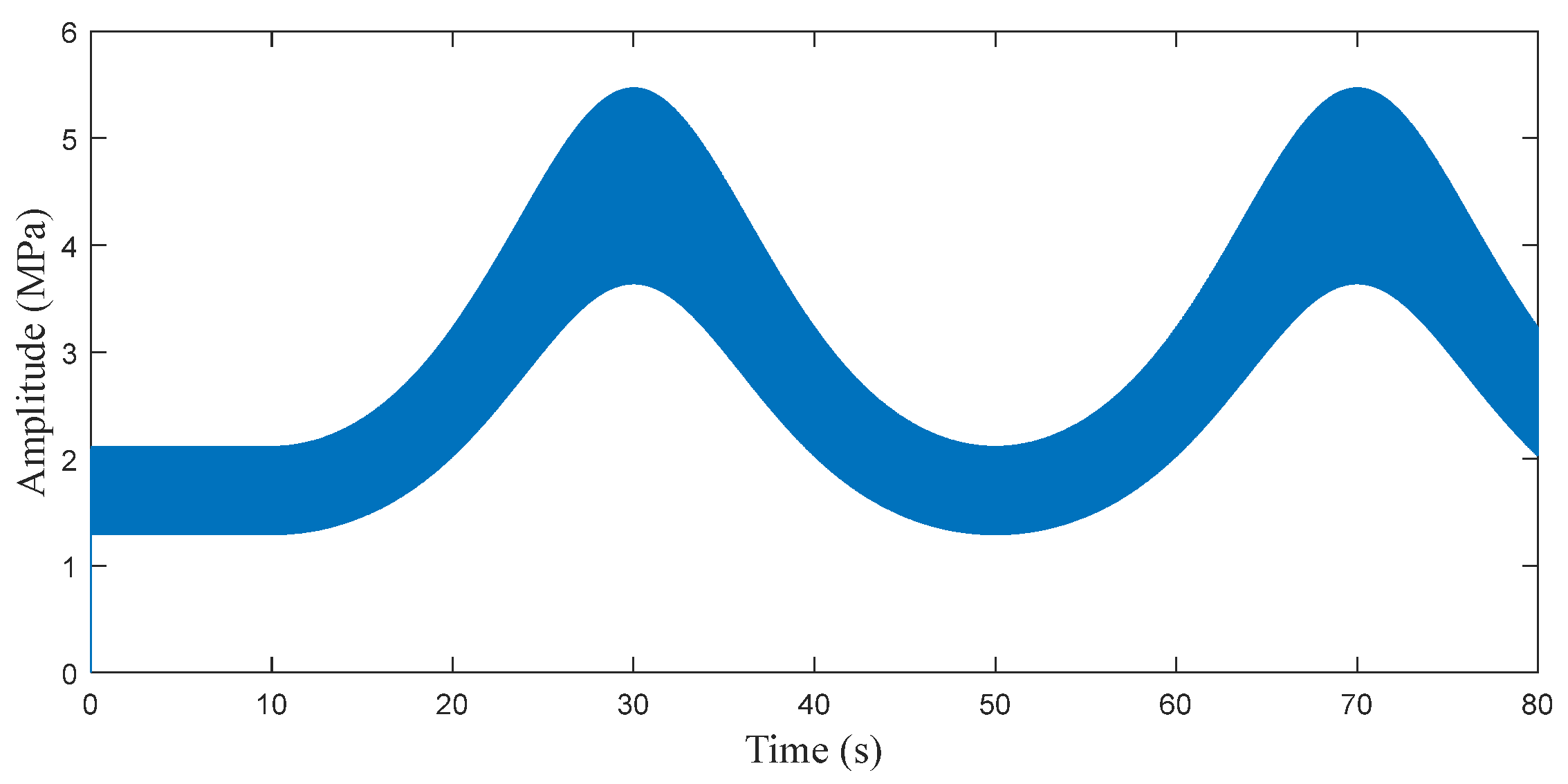
In practice, hydraulic system loads in ships are often fluctuating. This section aims to verify the robustness and adaptive tracking capability of the algorithm under non-stationary operating conditions by dynamically changing the opening of the load orifice. In the simulation experiment, the average pipeline pressure remains at 1.7 MPa, and the pulsation signal is composed of a fundamental frequency (150 Hz) and its second harmonic (300 Hz), with a total pulsation amplitude of 0.4 MPa. The total simulation duration is 80 s. Variable Orifice 2 remains in a “constant opening” state for the first 10 s, after which it enters a “variable opening” state, with its opening signal defined by Equation (23):

$$C_{\nu alve2}(t)=\left\{\begin{array}{ll}1& t\in [0,10)\\ 0.8-0.2sin\left(2\pi \cdot 0.025\cdot (x-20)\right)& t\in [10,80]\end{array}\right.$$

(23)

In the case where no control is applied throughout the entire process, the pressure sensor readings are shown in Figure 8. As seen in the figure, with the dynamic adjustment of the orifice opening, the average pipeline pressure fluctuates accordingly. Furthermore, the fluid pulsations consistently maintain a high level and do not weaken due to load changes, providing a complex background environment for verifying the adaptability of the algorithm.

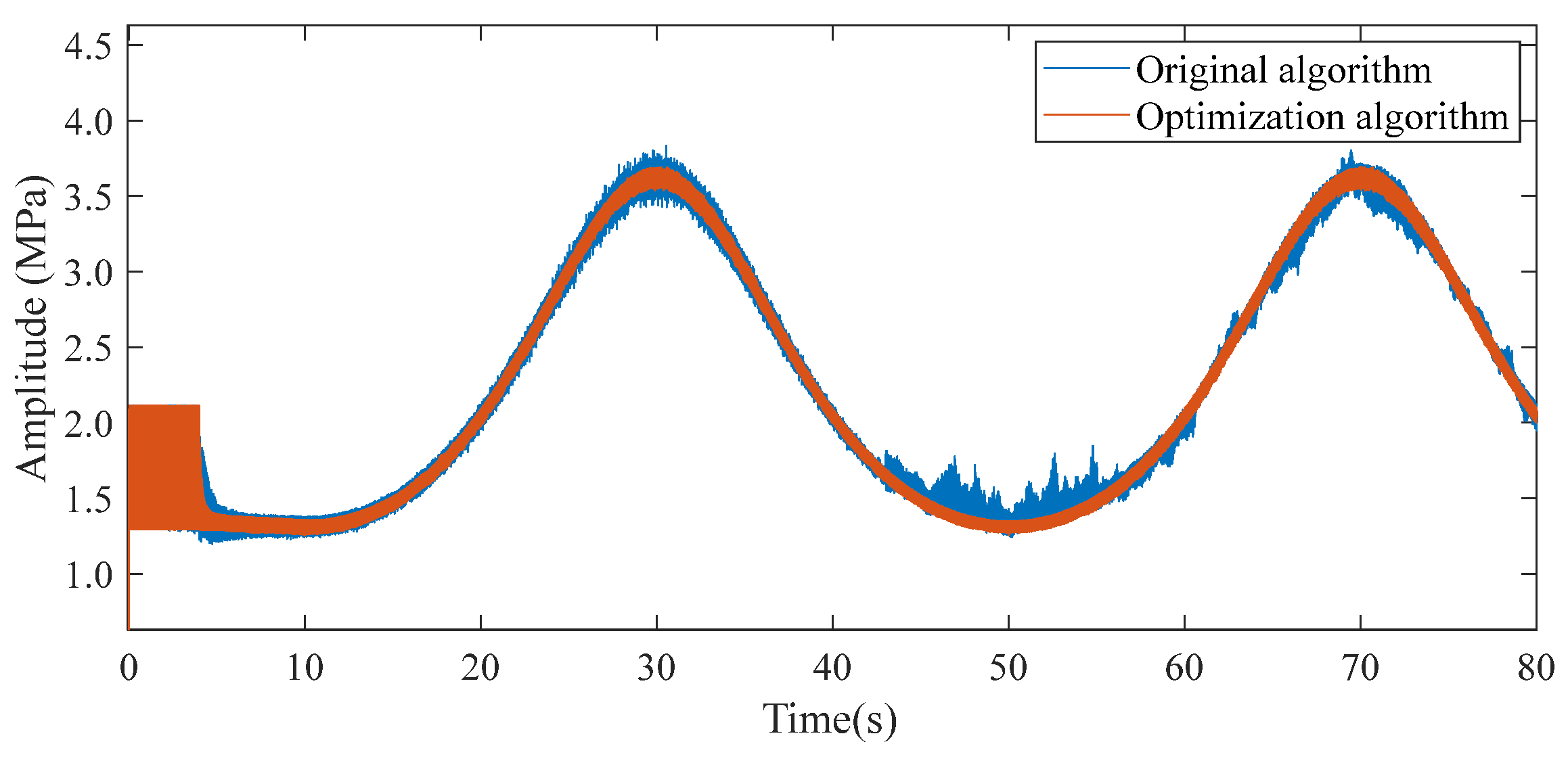
To verify the suppression capability of the algorithm under non-stationary conditions, the system switches to active control logic at t = 4 s. A comparison of the control effects between the traditional algorithm and the optimized algorithm is shown in Figure 9.

At the moment control is activated at t = 4 s, both algorithms can rapidly identify pulsation characteristics and generate a suppression effect. When the load begins its dynamic switching for t > 10 s, the optimized algorithm demonstrates stronger real-time parameter adaptability, enabling it to precisely track the pressure drift caused by load variations and maintain the stability of the control gain. Observing the waveforms in Figure 9, the traditional algorithm exhibits significant overshoot and a longer re-convergence time at points where the load changes substantially. In contrast, throughout the entire process of load fluctuation, the residual pulsation envelope of the optimized algorithm is smoother and thinner, indicating stronger control stability.

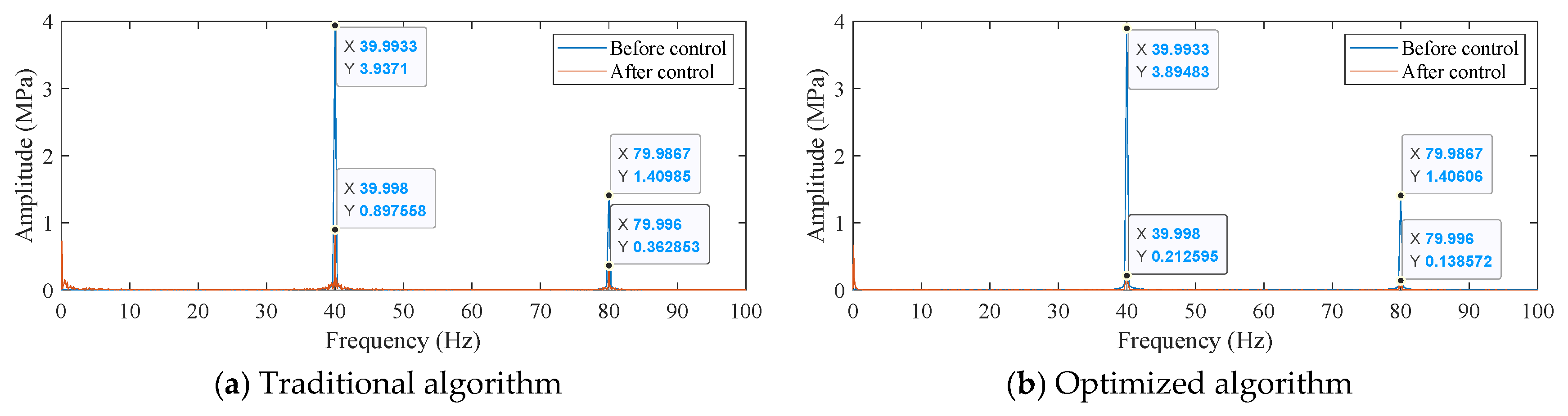
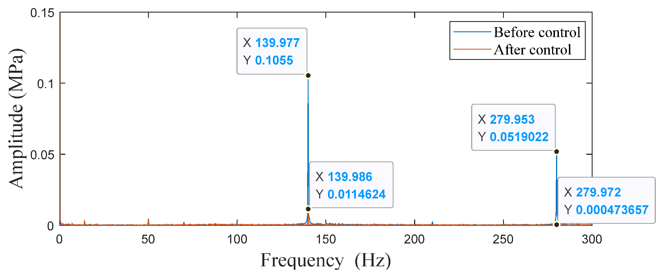
Figure 10 presents the comparison of pressure spectra for each control strategy under variable-load conditions.

Table 4. Comparison of pulsation control effects under a time-varying load environment.

Type	40 Hz			80 Hz
	Amplitude Before Control (MPa)	Amplitude After Control (MPa)	Attenuation Rate	Amplitude Before Control (MPa)	Amplitude After Control (MPa)	Attenuation Rate
Traditional algorithm	3.9371	0.8976	77.20%	1.4099	0.3629	74.26%
Optimized algorithm	3.8948	0.2126	94.54%	1.4061	0.1386	90.14%

provides a detailed quantitative listing of the amplitude changes and corresponding attenuation rates at the characteristic frequencies (40 Hz and 80 Hz) of the system. Although the variable-load environment significantly increases the complexity and control difficulty of the system, the optimization algorithm still achieves a significant lead of 17.34% and 15.88% in the attenuation rate at 40 Hz and 80 Hz, respectively, compared to the traditional algorithm. This comparative result strongly proves that the optimization algorithm proposed in this paper not only has extremely high steady-state control accuracy but also has excellent dynamic response speed and strong robustness, which can effectively overcome external disturbances and calmly cope with the complex and variable actual service conditions of the hydraulic system.

To further investigate the specific contribution of each module within the proposed optimized algorithm to the suppression performance, detailed simulation analyses were conducted separately on the variable-step-size module, the prediction error filter, and the variable-power white-noise signal.

4.2.1. Analysis of Variable Step-Size Effect

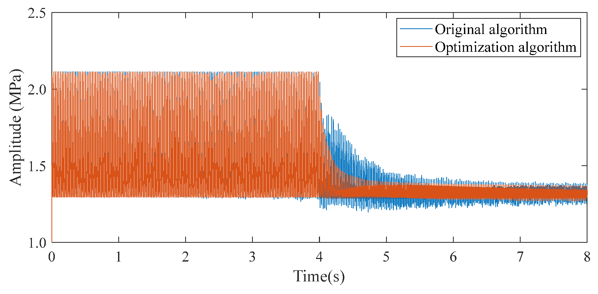
The core function of the variable step-size module is to resolve the contradiction between convergence speed and steady-state error. Figure 11 shows the localized magnified waveform (0–8 s) at the moment control is engaged at t = 4 s.

From the magnified view, it can be observed that after the traditional algorithm with a fixed step size is engaged at 4 s, the pressure envelope contracts relatively slowly. In contrast, after introducing the variable step-size module, the algorithm employs a large step size in the initial stage to achieve rapid optimization and automatically reduces the step size as it approaches a steady state to suppress misadjustment noise.

Experimental data indicate that the variable step-size module shortens the system’s convergence time from 1.9 s to 0.3 s, significantly enhancing the response sensitivity of the active control system and ensuring a rapid suppression capability against sudden pulsations.

4.2.2. Analysis of the Decoupling Effect of the Prediction Error Filter

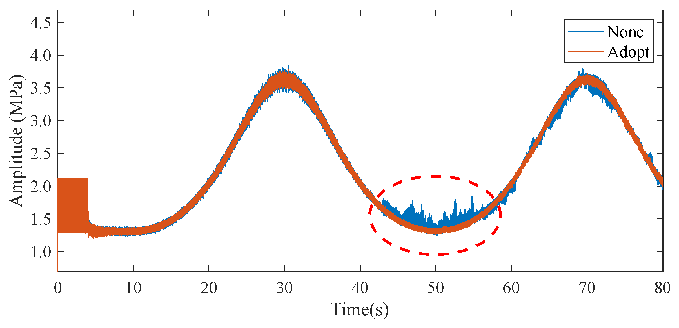
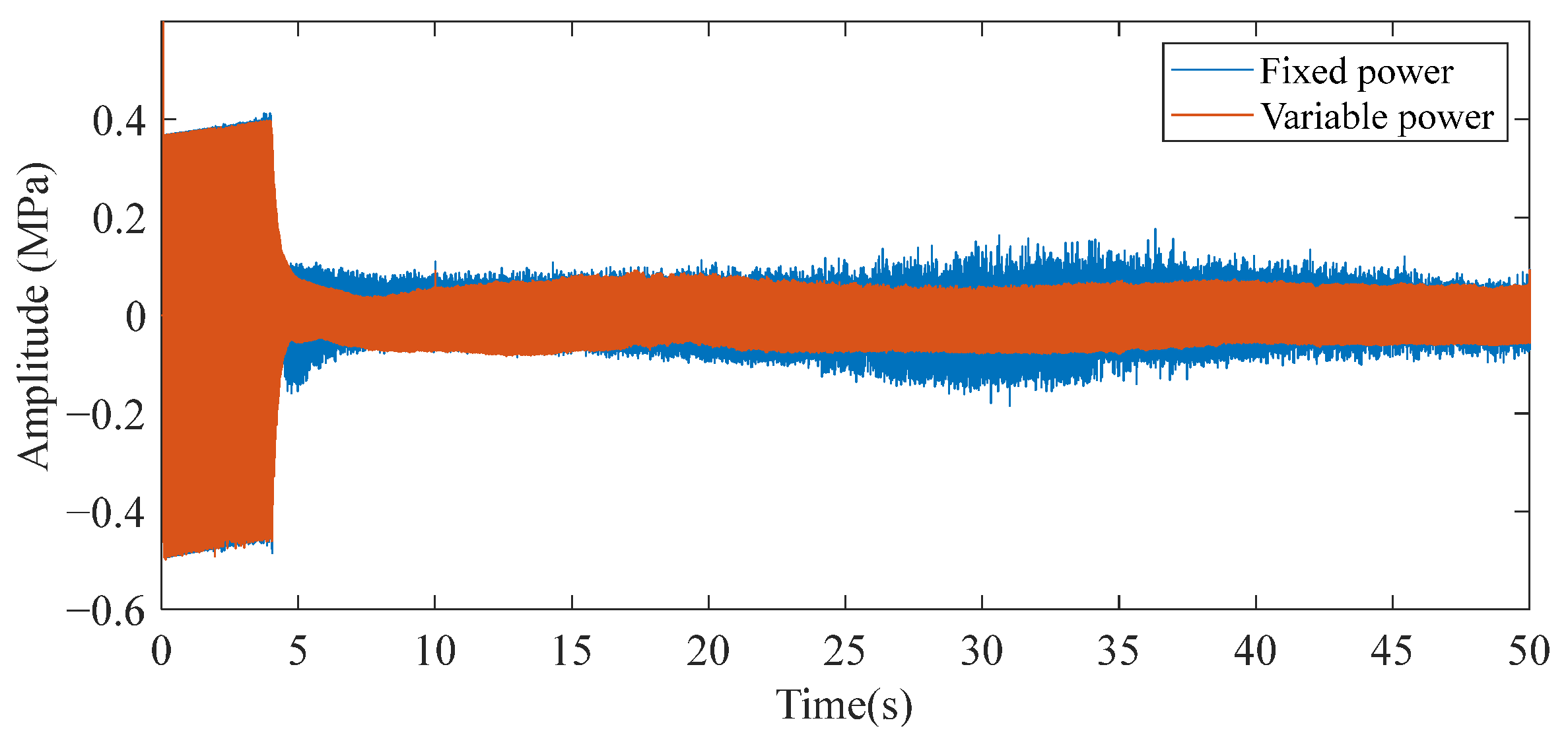
While maintaining the activation of the variable step-size module, the next step is a comparative analysis of the control performance before and after the introduction of the prediction error filter. This module is primarily used to extract pulsation characteristics in advance and filter out irrelevant interference under variable-load conditions. A comparative experiment was conducted to evaluate whether to employ prediction error filtering for decoupling, and the simulation results are shown in Figure 12.

From the figure, it can be clearly observed that the two algorithms, one using prediction error filtering for decoupling (orange curve) and the other without decoupling (blue curve), exhibit significant differences in pressure control. The overall trends of the two curves are basically consistent, indicating that the prediction error filtering decoupling strategy does not alter the fundamental dynamic characteristics of the system, thereby ensuring control stability. Specifically, in the low-pressure region (45–60 s), the pressure fluctuations of the decoupling algorithm are noticeably smaller than those of the traditional algorithm, resulting in a smoother curve. The pressure fluctuation range is reduced from ±0.5 MPa to approximately ±0.1 MPa, with the time-domain peak-to-peak value attenuated by 80%.

4.2.3. Analysis of Variable-Power White-Noise Effect

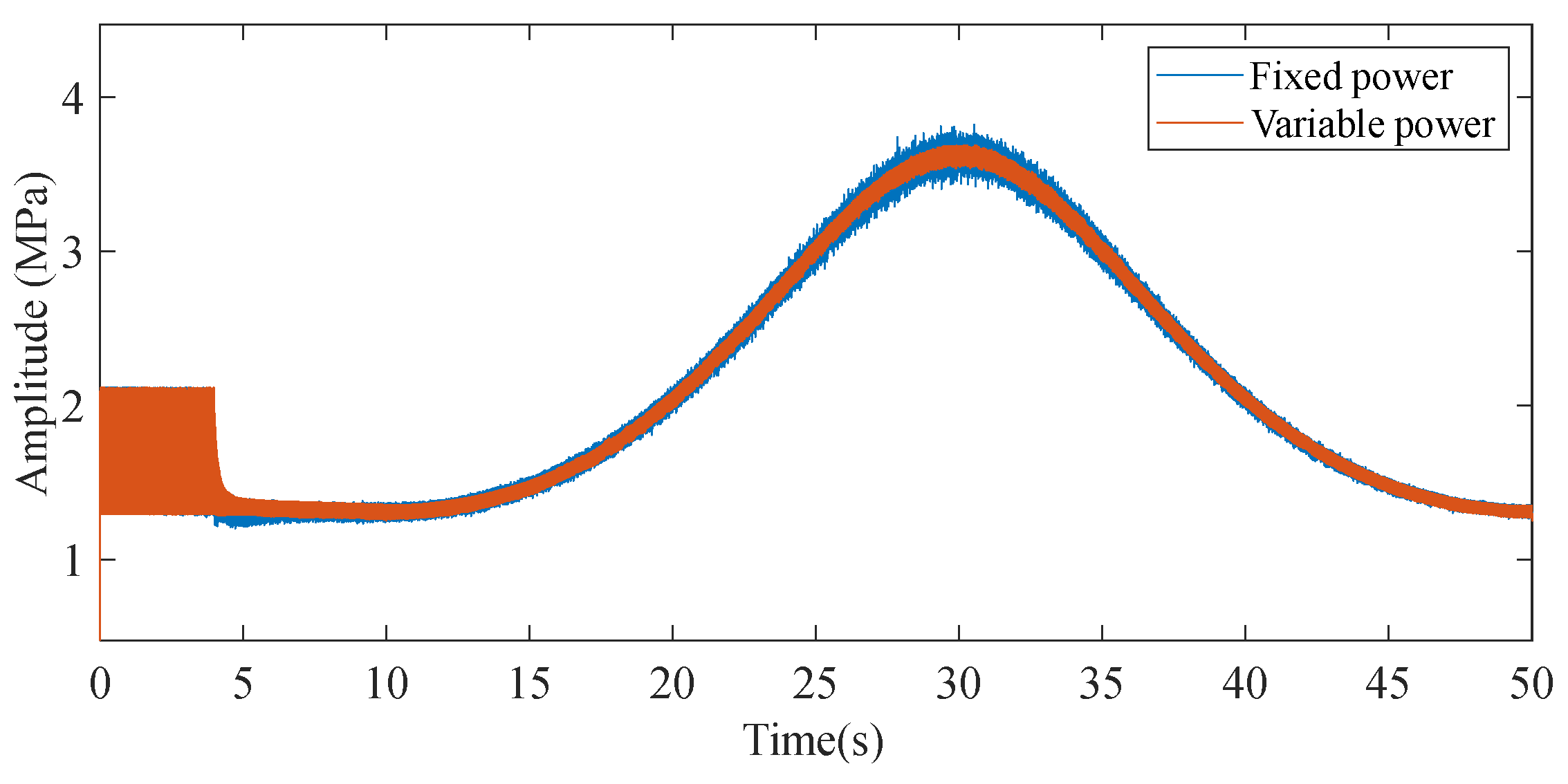
To verify the role of the variable-power white-noise module in improving time-domain control effectiveness, two sets of simulation experiments were designed for comparison. One set employs excitation white noise with a fixed power, where the power factor $a=15$, and the white-noise signal is expressed as in Equation (24). The other set utilizes excitation white noise with variable-power, with power factors $a_{\max }=20$ and $a_{\min }=0.01$, and the white-noise signal is expressed as in Equation (25), “$rand(1)$” represents a random number ranging from 0 to 1. The gain for both sets of white noise is 0.02, and both simulations utilize the variable step-size module and the prediction error filtering decoupling strategy.

$$WN=15\times 0.02\times rand(1)$$

(24)

$$WN=({\displaystyle \frac{20-0.1}{P_{\max }-P_{\min }}}\left(P-P_{\max }\right)+20)\times 0.02\times rand(1)$$

(25)

The simulation results are shown in Figure 13. From the time-domain curves, it can be observed that in the low-pressure segments, there is no significant difference in the peak-to-peak pressure values between control using fixed-power white-noise and variable-power white-noise. However, in the high-pressure segments, the peak-to-peak pressure values under variable-power white-noise control are significantly smaller.

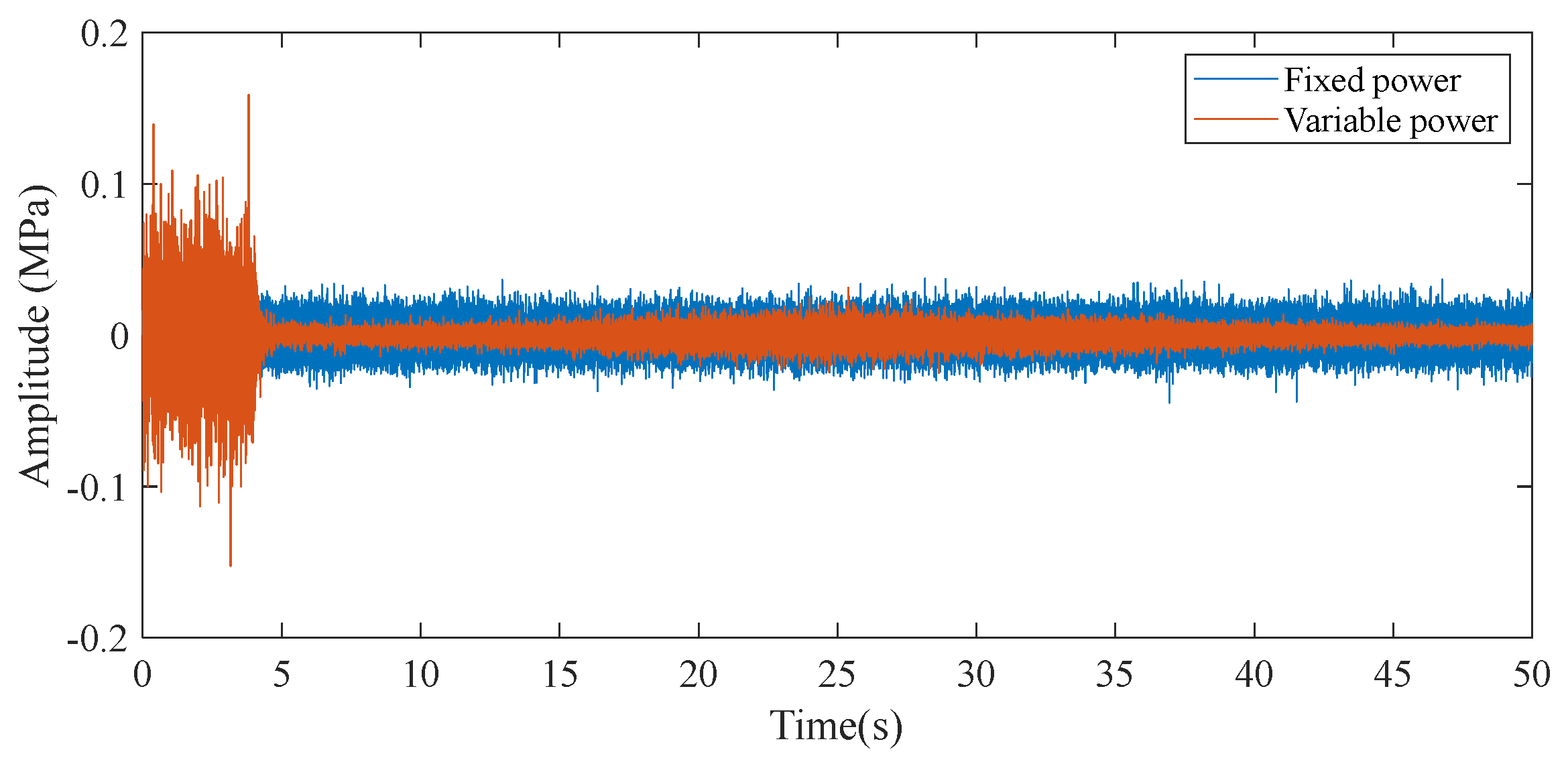
The time-domain curves of the pure pulsation signal (the original pulsation signal after removing the mean pressure) during the control process are shown in Figure 14. Three time points-10 s, 20 s, and 30 s-were selected to calculate the peak-to-peak pressure values for quantitative comparison; the results are presented in

Table 5. Peak Pressure values before and after “constant-power white-noise” control.

Time (s)	Control the Peak-to-Peak Value of the Pre-Pressure (MPa)	Controlled Post-Pressure Peak-to-Peak Value (MPa)	Attenuation Rate
10	0.8175	0.1506	81.57%
20	1.2148	0.1914	84.24%
30	1.8235	0.3055	83.24%

and

Table 6. Peak-to-peak pressure values before and after “variable-power white-noise” control.

Time (s)	Control the Peak-to-Peak Value of the Pre-Pressure (MPa)	Controlled Post-Pressure Peak-to-Peak Value (MPa)	Attenuation Rate
10	0.8175	0.1267	84.51%
20	1.2148	0.1317	89.16%
30	1.8235	0.1309	92.82%

. It is evident that at 10 s, 20 s, and 30 s, the time-domain attenuation using variable-power white noise is significantly greater than that using constant-power white noise. Notably, at 30 s, where the system pressure is at its maximum, the time-domain attenuation achieved with variable-power white noise exceeds 90%.

Figure 15 illustrates the white-noise power amplitudes during the control process for both the fixed-power and variable-power white-noise algorithms. As shown in the figure, the white-noise power of the fixed-power control algorithm remains constant throughout, whereas the white-noise power of the variable-power control algorithm is adjusted in real time according to the magnitude of the pulsation signal. The system initiates control at 4 s. In the initial stage of control, a higher white-noise power is employed to improve the identification accuracy of the secondary path. Once the control algorithm converges, it can consistently maintain a lower white-noise power, thereby weakening the coupling interference between the modeling process and the control process.

4.3. Summary of Simulation Results

In this section, the proposed optimization algorithm (comprising the variable step-size module, prediction error filter decoupling, and variable-power white-noise module) was comprehensively verified using the MATLAB/Simulink R2021b and AMESim 2021 joint simulation platform. The primary conclusions are as follows:

(1)

Verification of Algorithm Effectiveness: Through simulation analysis under constant load conditions, the superior performance of the active control system in handling multi-frequency composite pulsations was verified. The results demonstrate that the optimized algorithm improves convergence speed by approximately 67.5% compared to the traditional algorithm (shortened from 0.4 s to 0.13 s) and achieves a steady-state suppression rate of 93.91%.

(2)

Module Function Analysis: Comparative ablation experiments confirmed that the variable-step-size module significantly balances convergence speed and steady-state precision; the decoupling module effectively improves the signal-to-noise ratio of the error signal; and the variable-power white noise ensures sustained convergence stability of the algorithm under complex excitations.

(3)

Adaptability to Complex Conditions: In the 80 s variable-load simulation, the algorithm exhibited excellent robustness, successfully tracking pressure fluctuations caused by changes in orifice opening in real time. This proves the potential of the optimized algorithm to handle dynamic operating conditions.

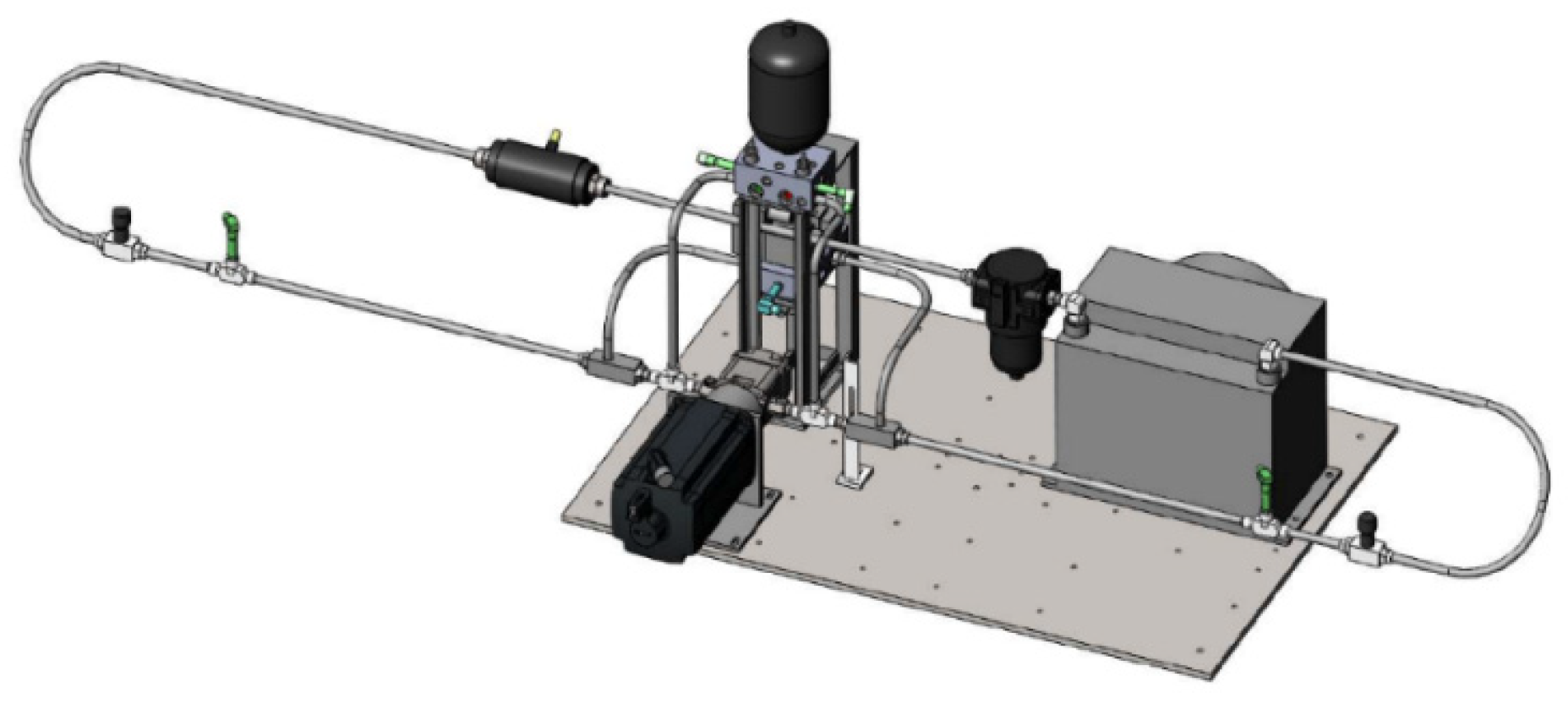
In summary, the simulation results theoretically verify the feasibility and superiority of the optimized algorithm in suppressing fluid pulsations. The next chapter will provide a detailed introduction to the composition of the experimental system and an analysis of the experimental results.

5. Experiment

5.1. Experimental Platform Construction and Component Selection

To verify the feasibility of the proposed algorithm in an actual physical system, a ship steering hydraulic system active pulsation suppression test rig was constructed. The system primarily consists of a servo motor, a gear-type fixed-displacement pump, a high-response servo valve, an orifice (simulating the load), and pressure pulsation sensors. The schematic diagram of the test rig is shown in Figure 16.

The system adopts a spill-type active control scheme: a gear pump serves as the primary pulsation source, featuring 10 teeth and driven by an adjustable-speed servo motor. The servo valve acts as the secondary pulsation source, connected across the pump outlet and the oil tank. By dynamically adjusting the overflow rate, it generates compensatory pulsation waves to suppress fluid pulsations within the pipeline. The physical distance between the secondary pulsation source and the primary pulsation source directly determines the causality and time delay of the control system. To meet the causality condition, we followed the principle of “as close to the pulsation source as possible” and arranged the servo valve at the proximal end close to the outlet of the hydraulic pump.

In a spill-type active control system, the selection of the secondary pulsation source (servo valve) must strictly satisfy the following two criteria:

(1)

Maximum Overflow Capacity: The maximum overflow capacity of the valve must be greater than the maximum amplitude of the fluid pulsations.

(2)

Response Frequency: The response frequency of the valve must be higher than the highest frequency of the fluid pulsations and their primary harmonic components.

The gear pump used in the experiment has a displacement of 20 mL/r, and the driving motor has a maximum speed of 1200 r/min. Based on the relationship Q = displacement × speed, the maximum average flow rate of the system is 24 L/min. Considering the number of pump teeth and the motor speed, the fluid pulsation frequency preset for this test rig can reach up to 200 Hz.

Based on these requirements, this study selects the DA03S direct-acting high-response servo valve manufactured by SANTEST, Osaka, Japan. The maximum flow rate of this valve is 40 L/min, with internal leakage of less than 1.7 L/min. Its frequency response is as high as 500 Hz. The actual performance parameters of this valve fully cover the frequency and flow range required by the experimental conditions.

The 3D model and physical photograph of the steering hydraulic system test rig are shown in Figure 17 and Figure 18, respectively.

5.2. Analysis of Experimental Results

5.2.1. Constant Load Conditions

The initial static pressure of the system was set to 3 MPa, the load orifice opening remained constant, and the pump speed was stabilized at 840 r/min. The results of the active control experiment are shown in Figure 19 and Figure 20.

From the error signal time-domain curve in Figure 19, it can be observed that the control algorithm exhibits excellent steady-state performance and convergence after being engaged. The convergence time is approximately 2 s, and the residual pulsations during the steady-state phase are maintained at a low level. Figure 20 illustrates the frequency spectrum comparison before and after control: the amplitude of the fundamental frequency pulsation signal was attenuated from 0.1055 MPa to 0.0114 MPa, achieving a pulsation attenuation of 89.1%, while the second harmonic pulsation was attenuated by 99%.

Experimental data demonstrate that under constant load conditions, the optimized algorithm is capable of achieving effective pulsation suppression.

5.2.2. Time-Varying Load Conditions

To verify the robustness of the algorithm in a non-stationary environment, system load fluctuations were simulated by dynamically adjusting the throttle valve opening. No control was applied during the initial phase of the experiment; active control was activated after 5 s, while simultaneously adjusting the throttle valve opening. The experimental results are shown in Figure 21 and Figure 22.

As seen in the time-domain plot, the algorithm achieves convergence within 2 s after activating active control and consistently maintains a high level of pulsation suppression. To further analyze the experimental results, a frequency spectrum comparison before and after control was plotted. As shown in Figure 23, the amplitude of the fundamental frequency pulsation signal was attenuated from 0.233 MPa to 0.019 MPa, reaching an attenuation rate of 91.8%, while the second harmonic pulsation was attenuated by 95%.

The time-frequency representation of the pressure signal in decibel scale during the control process, obtained via Short-Time Fourier Transform (STFT), is shown in Figure 24. The control algorithm effectively suppresses the fundamental and second harmonic pulsation components in the hydraulic system and maintains stable control performance even as the pressure changes.

Experimental data demonstrate that the optimized algorithm can converge rapidly and maintain stable control performance in a variable-load environment, validating the effectiveness and feasibility of the proposed active control scheme.

6. Conclusions

This paper proposes a three-level suppression strategy to address the coupling interference problem of active control filters in ship hydraulic systems. In the signal dimension, the prediction error filtering decoupling method is adopted. Through the delay prediction filter, the modeling process and the control process are decoupled, and the influence of the control signal on the identification of the secondary channel is filtered out, resulting in an 80% reduction in the peak-to-peak value in the time domain. In the amplitude dimension, a variable-power white-noise excitation strategy is employed, where the excitation power is dynamically adjusted according to the system pressure to reduce the interference of the modeling process on the control process. In the time dimension, an improved variable-step-size FxLMS algorithm with dual-nonlinear function collaborative coupling is proposed. Through the collaborative effect of rational fraction terms and exponential terms, the step size is finely and adaptively adjusted, accelerating the algorithm convergence and shortening the convergence time of the interference between the two, with the convergence time being shortened by more than 80%. The simulation and experimental results show that this collaborative optimization strategy effectively suppresses the coupling interference between the control filter and the modeling filter, achieving more than 90% attenuation of the line-spectrum pulsation. Compared with traditional algorithms, the proposed optimization algorithm exhibits excellent robustness and adaptability under various operating conditions, significantly improving the pressure pulsation suppression accuracy of ship hydraulic systems and achieving superior pulsation attenuation effects.

Although the multi-strategy collaborative optimization algorithm proposed in this paper has demonstrated excellent adaptive ability and steady-state accuracy in suppressing the pulsation of the ship hydraulic system, the practical engineering application of this active control system is still limited by its physical hardware characteristics. Firstly, high-precision active control relies on high-frequency response pressure sensors and actuators, which increases the system complexity. Secondly, the system achieves pressure damping by throttling and discharging fluids, and this irreversible process generates heat loss. In future long-term engineering applications, thermal balance analysis needs to be introduced. Moreover, due to the current experimental conditions, the algorithm in this paper has mainly been verified for specific power and pump types (such as spur pumps). When the system scale is significantly enlarged, or a pump with different initial pulsation characteristics (such as helical pumps) is used, the acoustic boundaries and fluid inertia of the system will change. Although the online identification algorithm in this paper has certain adaptive tracking capabilities, when facing large-scale hardware platform differences, it is still necessary to specifically evaluate the physical flow capacity of the actuator and the bandwidth limit of the algorithm. This is the focus of the next stage of research.