Physics-Prior-Augmented Deep Learning for Acoustic Convergence Zone Identification in Data-Scarce Marine Environments

Abstract

High-precision identification of acoustic convergence zones (CZs) and acoustic shadow zones (SZs) is a core prerequisite for deep-sea sonar performance prediction and long-range underwater target detection. However, in data-scarce marine environments, traditional acoustic identification methods suffer from high environmental sensitivity and significant computational costs, while pure data-driven deep learning methods face dilemmas such as a lack of physical consistency and poor generalization on small samples. To address these issues, a three-level cascaded recognition framework based on physics-prior-augmented deep learning is proposed in this paper, enabling accurate segmentation of CZs and intelligent classification of sound field types under data-scarce scenarios. In this framework, physical acoustic principles are incorporated exclusively as priors through a training dataset generated by a Gaussian beam acoustic propagation code (Bellhop) and through hand-crafted geometric features derived post hoc from the initial segmentation outputs. Taking a typical deep-sea area in the Northwest Pacific Ocean as the research object, a hybrid dataset comprising 5000 simulated transmission loss images and 500 simulated images from a geographically distinct sea area is constructed. The sound field is categorized into four types: strong convergence, usable convergence, weak convergence, and shadow zone. In the first stage, the ResNet-34 backbone is improved by integrating deformable convolution and a global statistical feature module, which, combined with a joint loss function, achieves high-precision pixel-level segmentation of CZs and SZs, with the regional gray contrast reaching 86.9%. In the second stage, a customized dual-channel VGG16 architecture is designed to fuse the extracted geometric priors and visual features, achieving a sound field classification accuracy of 89.91%. In the third stage, a hybrid data augmentation technique combining Mixup and convolutional autoencoder is adopted alongside a transfer learning strategy to mitigate the data scarcity under cross-domain conditions, boosting the small-sample classification accuracy to 84.45%. The experimental results demonstrate that the models in each stage of the proposed framework significantly outperform traditional methods and baseline networks. This study provides a novel methodology and technical support for intelligent sound field identification in data-scarce marine environments. Finally, the core contributions and current limitations are summarized, and future research directions, such as constructing a dynamic hydrological parameter feedback mechanism and identifying three-dimensional complex sound fields, are prospected.

1. Introduction

The complexity of the marine acoustic environment, particularly the non-uniform distribution of acoustic energy in deep-sea sound channels, makes underwater information perception challenging [1]. In the deep-sea environment, due to the refraction effect of the sound-speed profile (SSP), acoustic energy periodically converges near the sea surface to form high-gain convergence zones (CZs), while acoustic shadow zones (SZs) with extremely low energy distribution exist between these zones [2]. This unique spatial distribution law is not only a core indicator for predicting the performance of sonar systems but also an important basis for long-range detection, positioning, and tracking of underwater targets. With the increasing complexity of naval sonar performance assessment and underwater acoustic surveillance, achieving high-precision, real-time intelligent classification of acoustic field states is of great military engineering value and scientific research significance for optimizing sonar deployment and improving long-range early warning capabilities [3]. However, the real marine environment is affected by dynamic processes (such as internal waves and mesoscale eddies), and acoustic propagation paths exhibit high nonlinearity and spatiotemporal variability, which means traditional identification methods relying on static environmental models face enormous bottlenecks in practical applications [4].

Research on marine CZs began in 1961 when Hale mapped acoustic ray diagrams using experimental data to determine their geometric positions [5]. In subsequent decades, alongside advancements in computer technology and ocean exploration, the phenomenon of deep-sea CZs became widely recognized, with mesoscale processes such as ocean fronts and deep-sea eddies found to exert considerable impacts on their formation. For instance, Liu et al. and Zhang et al. systematically investigated the effects of these mesoscale phenomena on regional acoustic fields [6,7]. Historically, identifying these acoustic features has heavily relied on traditional analytical methods such as matched-field processing or ray-tracing models [8]. Although these methods possess a solid physical foundation, their performance is highly dependent on the accurate input of environmental parameters, such as the SSP and seabed sediment characteristics. Once environmental parameter mismatch occurs, identification accuracy decreases significantly. Furthermore, the high computational cost of large-scale scanning calculations severely limits their real-time application on mobile platforms [9]. Consequently, the rapid classification and robust extraction of CZ locations remains a critical research hotspot.

To address these operational inefficiencies, deep learning technologies, particularly convolutional neural networks (CNNs), have been introduced to process nonlinear acoustic images like transmission loss (TL) plots. These data-driven techniques effectively extract complex image texture features and have been widely applied in underwater acoustic target recognition [10,11,12,13]. More recently, advanced physics-guided or structure-aware frameworks have significantly accelerated the precision of acoustic field modeling; for instance, Mallik et al. proposed a convolutional recurrent autoencoder network to effectively learn reduced-dimensional representations of complex physical data for far-field TL distributions [14], and Yoon et al. developed a physics-informed neural network incorporating parabolic-equation envelope functions to successfully resolve the gradient convergence challenges caused by rapidly fluctuating acoustic phases [15]. While these breakthroughs have vastly elevated the capacity for continuous sound field prediction, expanding deep learning to the intelligent classification and structural boundary identification of macroscopic acoustic feature zones (such as CZs and SZs) still encounters distinct challenges. On one hand, standard classification backbones often lack explicit physical consistency constraints: operating as pure data-driven black boxes, they may ignore inherent physical principles like sound ray bending, leading to identified morphological features that fundamentally violate acoustic laws. On the other hand, these classification models face a severe small-sample generalization dilemma under restricted data conditions. Due to the prohibitive costs of marine experiments, labeled in situ acoustic transmission loss measurements are virtually nonexistent for most operational areas, and researchers must rely on simulated data generated by physics-based propagation models. Consequently, networks trained primarily on a single simulation domain exhibit pronounced performance degradation when transferred to geographically distinct target domains, struggling to adapt to the substantially different energy dispersion and morphological distributions induced by region-specific oceanographic conditions.

To overcome the severe constraints of data scarcity and domain shift, transfer learning has emerged as a crucial technical approach. Prior studies have demonstrated its efficacy in processing low-level statistical information and resolving sparsity issues in underwater target recognition and sound-source distance estimation [16,17,18,19,20,21]. However, the application of transfer learning in the broader marine acoustic field remains relatively limited and has yet to be comprehensively expanded to complex-feature-region classification tasks. Therefore, determining how to effectively integrate acoustic physical priors into deep learning architectures and leverage transfer learning technologies to bridge the gap between a data-rich simulated source domain and a geographically distinct, data-scarce simulated target domain has become an urgent key issue in marine intelligent identification.

More recently, several related advances have emerged in adjacent domains. In deep-sea convergence zone analysis specifically, Li and Li (2023) modified a ResNet-50 to classify target depth from 1D echo spectra in CZ environments, achieving a 17% improvement over traditional matched-field processing [22]. For underwater acoustic image segmentation, Sun et al. (2024) proposed CGF-Unet, which integrates Transformer blocks into a UNet backbone for sidescan sonar semantic segmentation, leveraging self-attention to capture global context and achieving 89.3% mIoU [23]. In cross-domain few-shot learning, Cui et al. (2024) developed a contrastive learning framework for ship-radiated noise recognition that jointly optimizes source- and target-domain representations, reaching 76.93% accuracy in 5-shot settings [24], while Mohammadi et al. (2025) systematically demonstrated that ImageNet-pretrained CNNs can match or exceed audio-specific pretrained models for passive sonar classification under domain shift [25]. On the physics integration front, Chen et al. (2025) proposed a dual-physics-constrained PINN that embeds both normal mode and parabolic equation theories into the loss function for continuous acoustic field prediction [26]. Despite these advances, none of the existing works simultaneously address three interconnected challenges: pixel-level CZ/SZ segmentation from 2D TL images, physics-prior-augmented classification using hand-crafted geometric features, and cross-domain few-shot generalization via a controlled sim-to-sim proxy for real-world data scarcity.

To address the critical limitations of traditional analytical methods regarding environmental sensitivity and computational cost, as well as the inherent flaws of standard deep learning models regarding physical interpretability and small-sample generalization, this paper proposes a three-stage cascaded recognition framework that seamlessly integrates physics-prior augmentation with cross-domain transfer learning. The distinct methodological novelty of this cascaded architecture lies in its explicit decoupling and sequential fusion of physical feature parsing, semantic classification, and cross-domain adaptation. The primary objective is to guarantee high recognition accuracy by leveraging physics priors that are learned within the network through simulation-driven pretraining and geometric feature engineering, rather than as externally imposed PDE constraints.

To operationalize this framework, the research first introduces a structure-sensitive physical parser via an acoustic field region segmentation method. By enhancing a deep residual network to perceive sound ray density through optimized residual structures, the model achieves high-precision pixel-level segmentation of CZs and acoustic SZs within TL images, thereby explicitly extracting deterministic macroscopic geometric attributes. Building upon these precise segmentation outputs, a prior-augmented decision center is established by constructing a dual-channel classification model. This architecture systematically fuses the hand-crafted geometric priors extracted during the segmentation stage, specifically regional proportions and spatial coordinates, with raw visual textures. By strictly enforcing these macroscopic acoustic laws, this integration effectively resolves the misclassification dilemmas faced by traditional purely visual models when processing morphologically similar acoustic fields, thereby realizing a highly refined intelligent classification scheme. Furthermore, to address the ubiquitous challenge of data scarcity, a cross-domain transfer strategy functioning as a controlled sim-to-sim bridge is tailored for few-shot scenarios. A hybrid data augmentation technique combining Mixup and convolutional autoencoder is introduced to suppress overfitting during restricted training. Coupled with a hierarchical learning-rate-adjustment paradigm utilizing source-domain pretraining and target-domain fine-tuning, the proposed strategy successfully migrates the physics-constrained representations, achieving robust cross-domain adaptation from a data-rich simulated source domain to a geographically distinct, data-scarce simulated target domain, as a principled proxy for real-world deployment scenarios.

The remainder of this paper is organized as follows. Section 2 details the materials and methods, encompassing the study domain dataset construction, the structure-sensitive acoustic field semantic segmentation, the dual-channel classification fusing post hoc geometric physical priors and visual textures, the feature enhancement based on convolutional autoencoders, and the few-shot classification based on transfer learning. Section 3 presents the experimental results and analysis, covering the performance evaluation of the sound field region segmentation, the assessment of the dual-channel classification model, and the generalization validation under data-scarce scenarios. Finally, Section 4 and Section 5 discuss the methodological taxonomy of this study and conclude the paper by summarizing the core contributions and outlining future research directions.

2. Materials and Methods

2.1. Study Domain and Dataset Construction

This study focuses on a typical deep-sea area in the Northwest Pacific Ocean. Within this specific physical marine region, the spatial evolution of seawater sound speed with depth forms a typical deep-sea sound channel structure, with the channel axis depth typically distributed at approximately 1000 m. To comprehensively characterize the acoustic propagation characteristics of this area and establish a robust recognition model, systematic definitions of the key physical variables in the experiments are provided in this paper.

To simulate the acoustic radiation characteristics of a typical deep-sea submerged operation platform, the source depth is strictly positioned at 1000 m, which precisely aligns with the deep sound channel axis. Crucially, the source frequency is set to 50 Hz to capture the low attenuation characteristics of low-frequency sound waves during long-range propagation. It is worth noting that while conventional ray-geometric methods may face physical validity challenges at low frequencies (below 100 Hz) due to diffraction effects [8,27], the use of the Gaussian beam acoustic propagation code (Bellhop) at 50 Hz in this specific deep-sea study remains theoretically justified and methodologically appropriate. First, in our deep-sea environment, with a maximum vertical depth of 5000 m, the water depth-to-acoustic wavelength ratio remains sufficiently large ($H/\lambda \approx 167$), preserving the macro-scale geometric trajectory validity of the ray paths. Second, unlike rigid geometric rays, Bellhop’s geometric hat beams possess a finite beam width determined by the cross-section of ray tubes, thereby smoothing out unphysical singularities at caustics and extending the method’s low-frequency-applicability threshold. Most importantly, the downstream objective of our deep learning framework is image-based semantic segmentation and macro-pattern classification (identifying the general existence and spatial span of CZs), rather than requiring point-to-point coherent phase and absolute amplitude matching. Thus, Bellhop strikes an optimal operational balance, providing the necessary macroscopic physical realism while maintaining the computational efficiency required to generate a massive training dataset.

In terms of spatial scale, the range of acoustic propagation calculations in this paper is limited to a vertical profile with a horizontal distance of 0–100 km and a depth range of 0–5000 m. This spatial envelope is sufficient to fully cover the evolution process of at least one complete period of the CZ structure, thereby ensuring that the model can capture the periodic physical laws of acoustic field morphology.

The construction of the dataset in this study follows the principles of “reliable physical sources and multi-source data coupling”. To ensure the physical authenticity of the simulation calculations, the WOA18 global gridded reanalysis dataset released by the National Centers for Environmental Information (NCEI) was selected as the original input for the oceanic temperature and salinity fields [28,29]. This dataset integrates global in situ observational data collected up to 2018; specifically, the temperature and salinity data of the Northwest Pacific Ocean (120° E–160° E, 0° N–50° N), with a spatial resolution of 0.25° and a temporal resolution of quarterly, were adopted in this study. In terms of depth scale, WOA18 employs an unequal-interval layered structure (102 layers within the depth range of 0–5500 m), which can finely characterize the variations in sound-speed gradient near the thermocline and sound channel axis. By screening deep-sea points with seawater depth no less than 5000 m within this geographic range, a total of 13,747 sets of high-quality temperature and salinity data were obtained. Based on these data, 5000 sound TL images with high environmental diversity were generated using the Bellhop ray tracing model.

In the process of characterizing deep-sea sound field features, TL images can intuitively represent the propagation laws of the sound field and the loss regions of sound rays. Therefore, this study employs the Bellhop model to calculate the acoustic TL. As an efficient sound propagation model in underwater acoustics based on ray tracing and geometric beam approximation, the Bellhop model is widely used to compute TL and multipath structures in marine environments. When determining ray coordinates, Bellhop obtains the amplitude and sound pressure by solving the ray equations. For a general cylindrically symmetric system, the ray equations are expressed as in Equation (1):

$$\left\{\begin{array}{c}{\displaystyle \frac{dr}{ds}}=c\xi \left(s\right),{\displaystyle \frac{d\xi }{ds}}=-{\displaystyle \frac{1}{c^2}}{\displaystyle \frac{\mathsf{\partial }c}{\mathsf{\partial }r}},\hfill \\ {\displaystyle \frac{dz}{ds}}=c\zeta \left(s\right),{\displaystyle \frac{d\zeta }{ds}}=-{\displaystyle \frac{1}{c^2}}{\displaystyle \frac{\mathsf{\partial }c}{\mathsf{\partial }z}}.\hfill \end{array}\right.,$$

(1)

where $r\left(s\right)$ and $z\left(s\right)$ represent the ray coordinates in a cylindrically symmetric system, s denotes the arc length along the ray, and $c(r,z)$ is the sound-speed distribution. This equation is solved via numerical integration to obtain the curvature variation of the ray trajectory, thereby reflecting the influence of the sound-speed gradient on the propagation path.

The calculation of TL is based on the superposition of the sound-pressure field. Bellhop calculates the sound pressure $p(r,z)$ via the superposition of geometric beams and converts it into TL, as defined in Equation (2):

$$TL(r,z)=-20log\left|{\displaystyle \frac{p(r,z)}{p_0(r=1)}}\right|,$$

(2)

where $p_0$ is the sound-pressure intensity at a typical reference distance. For incoherent TL, the model superimposes the energy of each sound ray and ignores the phase information, and the generated images are more adaptable to complex multipath scenarios. In addition, the output TL images can be processed into ray trajectory plots and TL contour maps after point cloud or digitalization processing, providing multidimensional visualization support for deep-sea sound field feature analysis.

The environment file of the Bellhop model defines the physical boundary conditions and medium parameters of sound propagation. The sound-source frequency is set to 50 Hz and the water medium is defined as a single layer, where nmedia equals 1. The SSP adopts the SVW option for piecewise linear interpolation covering from the sea surface to a depth of 5000 m. The minimum sound speed occurs at the mid-deep layer around 1200 m, forming the deep-sea sound channel axis. The seabed is modeled as a sandy sediment layer with a density of $1.8{\mathrm{g}/\mathrm{cm}}^3$ and a P wave velocity of $1600\mathrm{m}/\mathrm{s}$. While acoustic propagation under sub-critical depths is inherently sensitive to these sediment variations, which can contribute to apparent CZs via bottom-bounce paths [8], the resulting morphological uncertainties are mathematically accommodated by the hybrid data augmentation strategy in the subsequent visual feature space. The sound source is positioned at a depth of 1000 m while the receiver grid spans the full water depth of 0 to 5000 m over a horizontal range of 0 to 100 km. The coherent TL calculation mode, denoted as CG (i.e., coherent transmission loss with geometric hat beams), is adopted, with emission angles ranging from $-20.3°$ to $20.3°$. The ray-tracing step size is set to 50 m and the computational domain boundaries are defined by a depth box of 5500 m and a range box of 100 km to guarantee accurate calculation of ray curvature, which is particularly critical for the periodic repetition of CZs in long-range deep-sea propagation scenarios.

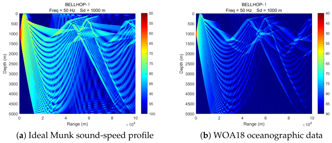
It must be explicitly clarified that the Munk profile is utilized in this study solely as an analytic canonical benchmark to illustrate the theoretical formation of convergence zones, rather than as a “ground truth” representing any specific real-world ocean environment. Figure 1a displays the sound TL image for the ideal Munk profile, which was generated using the aforementioned parameters, where the horizontal axis represents the propagation distance from 0 to 100 km, the vertical axis represents water depth from 0 to 5000 m, and the color bar indicates the sound energy loss intensity. The light-colored regions with TL less than 80 decibels in Figure 1a correspond to acoustic CZs, which appear as periodic high-energy stripes in the 20 km to 60 km range. The blue regions with TL greater than 90 decibels represent acoustic SZs, which are formed by the combined effects of seabed reflection loss and sound ray refraction. Figure 1b shows the TL image generated using the WOA18 oceanographic climatological data. In this specific image, the CZs are mainly concentrated in a small area near a horizontal distance of 40 km and a depth of 1000 m. This positional difference primarily arises from the depth deviation of the sound channel axis between the WOA18-derived SSP and the ideal Munk model. Real oceanographic environments, such as those derived from WOA18 profiles or in situ measurements, deviate substantially from the canonical analytic Munk form, leading to highly complex and variable sound field morphologies. Furthermore, this shift is exacerbated by discrepancies between the in situ and theoretical values of the seabed sediment absorption coefficient.

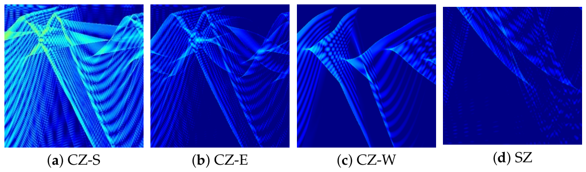
To achieve accurate evaluation of the detection efficiency of oceanic sound fields, this study categorized the sound field images into four types of labels with clear acoustic physical significance, according to the geometric morphology and intensity characteristics of energy distribution in the TL images, as visually illustrated in Figure 2. The classification criteria not only referred to the attenuation degree of acoustic energy but also incorporated the gain requirements for target detection in sonar engineering [30,31]. The detailed quantitative definitions and classification criteria for each type are presented in

Table 1. Definitions and classification criteria of the four acoustic field types.

Sound Field Type	Definition
Strong convergence type	The proportion of convergence zone exceeds 50%, with a significant enhancement of sound pressure
Exploitable convergence type	The proportion of convergence zone is between 20% and 50%, characterized by spatially continuous acoustic energy that permits stable sonar tracking
Weak convergence type	The proportion of convergence zone is between 20% and 50%, characterized by fragmented and scattered acoustic energy, unsuitable for stable tracking
Shadow zone type	The proportion of convergence zone is less than 20%, with uniform distribution of sound field energy

. To eliminate subjective ambiguity in overlapping intervals, the classification is strictly governed by the area proportion and the physical spatial continuity of the acoustic energy (i.e., contiguous refractive caustics versus fragmented multipath bounces). Because the dataset was uniformly annotated by the authors as the definitive ground truth based on these morphological guidelines, rather than by independent blind raters, multi-rater reliability statistics (e.g., Cohen’s $\kappa$) are inapplicable. Furthermore, while continuous regression models provide high-precision predictions for specific acoustic parameters [2], our discrete 4-class scheme is explicitly optimized for naval tactical decision making and acts as a robust statistical regularizer to prevent overfitting under data-scarce constraints.

To evaluate the framework’s cross-domain generalization capability under realistically data-scarce conditions, an additional 500 simulated TL images were generated using WOA18 oceanographic data from the South China Sea region (105° E–125° E, 0° N–25° N). These images, derived from a geographically distinct maritime environment, serve as a controlled proxy for the practical scenario in which extensive in situ acoustic measurements from a new operational area are unavailable—a pervasive challenge in underwater acoustics that motivates the entire transfer learning design. The South China Sea dataset is deliberately restricted to 500 samples to emulate the few-shot learning regime. To mitigate the risk of model overfitting under this limited sample size, data augmentation, including mirror flipping, random rotation, and Gaussian noise injection, was applied before the fine-tuning phase. This “source domain–target domain” construction scheme—where the abundant Northwest Pacific data (5000 images) constitute the source and the scarce South China Sea data (500 images) constitute the target—provides a principled and reproducible experimental foundation for systematically evaluating cross-domain transfer learning under controlled yet realistic data constraints.

The complete dataset is partitioned as follows. For the Northwest Pacific dataset (5000 images), a stratified 70%/15%/15% split is adopted, yielding 3500 training, 750 validation, and 750 test samples. This split supports the supervised training and evaluation of both the Stage 1 semantic segmentation model and the Stage 2 dual-channel classification model. The Northwest Pacific training set further serves as the source domain for pretraining the Stage 3 transfer learning model. For the South China Sea dataset (500 images), a stratified 40%/20%/40% split is applied, producing 200 fine-tuning, 100 validation, and 200 test samples, dedicated exclusively to the target-domain adaptation and evaluation of the Stage 3 few-shot transfer learning experiments. All splits are performed via stratified random sampling to preserve the natural class distribution across the four acoustic categories within each subset. The Northwest Pacific and South China Sea datasets are derived from geographically disjoint WOA18 profiles with no spatial overlap, ensuring complete physical separation between the source and target domains and eliminating any risk of data leakage. All performance metrics reported in this paper are evaluated exclusively on the respective held-out test sets, which remain unseen during the entire training and hyperparameter-tuning process.

2.2. Structure-Sensitive Acoustic Field Semantic Segmentation via Deformable Convolution

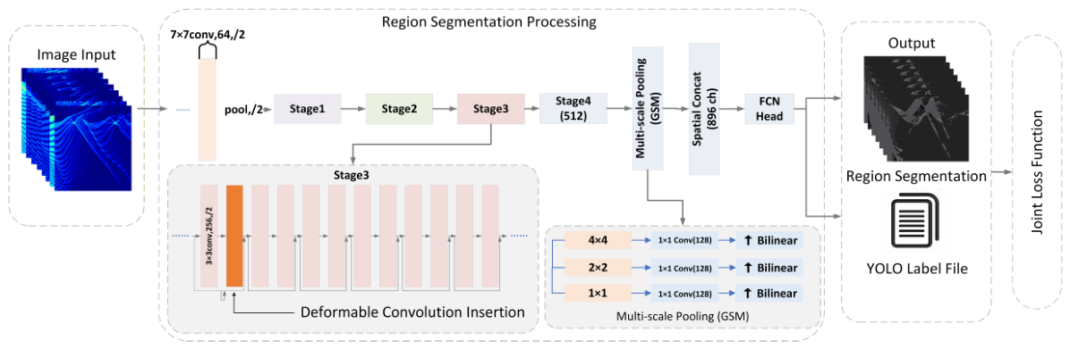
The physics-prior-augmented cascaded recognition framework proposed in this paper aims to address the challenges of physical mismatch and poor generalization in sound field recognition under complex marine environments. Following the logical architecture of geometric prior extraction, multi-source feature fusion, and cross-domain knowledge transfer, the framework achieves the transformation from raw sound propagation images to high-confidence classification results through three cascaded phases. The primary objective of the first phase is to accurately extract the geometric contours of CZs from complex TL images. To mitigate the nonlinear distortion induced by acoustic refraction, this study proposes a structure-aware improved ResNet-34 network. By integrating deformable convolution and a global statistical feature module, the model enables fine-grained pixel-level segmentation of the acoustic boundaries of sound fields. The architecture of the improved sound field feature region segmentation model is illustrated in Figure 3.

The ResNet-34 network incorporates a multi-layer residual structure, and this multi-level convolutional architecture can effectively capture both feature details and global information in conventional images [32]. However, deep residual networks are primarily designed for recognizing natural images and lack targeted optimization for the details and global information of simulated images [33]. To address this issue, two improvement schemes—shallow feature preservation and adaptive sampling—are integrated into the backbone network.

In natural-image processing, high-level semantic features of deep networks usually receive more attention. Nevertheless, in the sound field segmentation task, the images contain fewer features compared to natural images. Therefore, rather than relying on pyramidal skip connections that would reintroduce low-level texture noise into the physically smooth acoustic field, multi-scale acoustic context is captured at the bottleneck: after the final residual stage, a three-level adaptive pooling module extracts features at 4 × 4, 2 × 2, and 1 × 1 spatial granularities, which are concatenated with the original Stage 4 feature map to form a multi-scale representation at a single resolution level [34]. This design preserves global acoustic energy distribution information while avoiding the parameter overhead of a symmetrical decoder, which is crucial for maintaining generalization under the data-scarce conditions of marine acoustic applications [35].

To ensure the sensitivity of the network model to variations in sound ray density, deformable convolution is introduced into the residual blocks of Stage 3. By dynamically adjusting the sampling positions of the convolution kernel through learnable offsets in deformable convolution, the network’s recognition rate for regions with significant changes in sound ray density can be improved, along with the segmentation accuracy of proportion variations [36].

Deep-sea acoustic field images are often characterized by high local sound intensity and wide global distribution. Single-scale pooling operations tend to lose global density distribution information, resulting in blurred boundaries between sound SZs and CZs [37]. To this end, this paper designs a multi-scale global statistical feature module at the output of Stage 4. Through three-level pooling and feature rescaling mechanisms, the discrimination ability of the network model for sound SZs and CZs in the images is improved [38].

• Multi-scale pooling: given the Stage 4 output $F\in {\mathbb{R}}^{512\times S\times S}$, three parallel pooling branches are applied at different spatial scales, as shown in Equation (3):

  $$\begin{array}{cc}\hfill P_4& =\mathrm{AdaptiveAvgPool}2\mathrm{d}(F,(4,4))\in {\mathbb{R}}^{512\times 4\times 4}\hfill \\ \hfill P_2& =\mathrm{AdaptiveAvgPool}2\mathrm{d}(F,(2,2))\in {\mathbb{R}}^{512\times 2\times 2}\hfill \\ \hfill P_1& =\mathrm{AdaptiveAvgPool}2\mathrm{d}(F,(1,1))\in {\mathbb{R}}^{512\times 1\times 1}\hfill \end{array};$$

  (3)
• Each pooled branch is projected to 128 channels via a $1\times 1$ convolution, as defined in Equation (4):

  $$P_k^{\prime }={\mathrm{Conv}}_{1\times 1}(P_k,C_{\mathrm{out}}=128),k\in \{1,2,4\};$$

  (4)
• Bilinear upsampling restores each projected feature map to the Stage 4 spatial resolution $(S\times S)$, as expressed in Equation (5):

  $$U_k=\mathrm{BilinearInterpolate}(P_k^{\prime },(S,S))\in {\mathbb{R}}^{128\times S\times S};$$

  (5)
• The original Stage 4 features and the three upsampled branches are concatenated along the channel dimension to form a spatially enriched 896-channel feature map, as computed in Equation (6):

  $$F_{\mathrm{enriched}}=\mathrm{Concat}(F,U_4,U_2,U_1)\in {\mathbb{R}}^{896\times S\times S}.$$

  (6)

The global statistical feature module constructed by three-level pooling and spatial concatenation enables not only the global perception of the overall density baseline but also the fine identification of local high-density regions, effectively improving the ability of the network model to detect the boundaries between sound SZs and CZs.

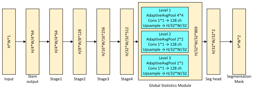
To transform the globally enriched feature representation into dense pixel-level predictions at the original input resolution, the proposed framework follows the FCN-32s paradigm: a purely convolutional prediction head operating at the bottleneck resolution, followed by a single bilinear upsampling that directly restores the original input dimensions. Specifically, the 896-channel feature map produced by the global statistics module (at 1/32 of the input resolution) is passed through a lightweight segmentation head consisting of three convolutional layers: a 3 × 3 convolution, reducing the channels from 896 to 256 (with BatchNorm and ReLU); a second 3 × 3 convolution, providing a further reduction to 128 channels (with BatchNorm and ReLU); and a final 1 × 1 convolution projecting to 2 channels, representing the CZ and SZ class logits. All three layers operate at the same 1/32 resolution, keeping the head computationally lightweight (approximately 0.5 M parameters). The resulting 2-channel logit map is then restored to the original input resolution via a single bilinear interpolation, yielding the final pixel-level segmentation mask. The complete spatial resolution and feature dimension flow through the architecture is illustrated in Figure 4. This design incorporates no skip connections from earlier stages: the multi-scale acoustic context has already been aggregated within the global statistics module at the bottleneck, and a direct single-step upsampling acts as an implicit regularizer that suppresses overfitting under data-scarce conditions.

The selection of a modified ResNet-34 backbone paired with this lightweight FCN upsampling head—as opposed to over-parameterized canonical segmentation baselines like U-Net or DeepLabv3+—is justified by the unique physical characteristics of ocean acoustic fields. Unlike natural images, which contain discrete, highly heterogeneous objects, sound TL images represent continuous energy fields with periodic, relatively uniform geometric strips. Heavy decoders utilizing extensive Atrous Spatial Pyramid Pooling (ASPP) or symmetrical heavy skip connections introduce massive parameter redundancy. In our data-scarce marine environment scenario, such over-parameterization severely elevates the risk of catastrophic overfitting. Our lightweight FCN-32s single-upsampling design actively suppresses overfitting and guarantees high computational efficiency for edge-sonar deployment while focusing the network’s capacity on structural density deformations.

Considering the particularity of the sound field feature region segmentation task, a joint loss function, $L_{\mathrm{Total}}$, is designed based on the fusion of global feature proportion and local details. Composed of the global area matching loss, denoted as $L_{\mathrm{GAML}}$, and the density gradient loss, denoted as $L_{\mathrm{ABFL}}$, this loss function is used to mitigate the increase in overall misjudgment rate caused by local misclassification.

The global area matching loss, denoted as $L_{\mathrm{GAML}}$, directly constrains the difference in global pixel proportion between the predicted region and the soft boundary label, forcing the network to learn the physical property of sound field energy conservation, as shown in Equation (7):

$$L_{\mathrm{GAML}}=|{\displaystyle \frac{{\sum }_{i=1}^N{p}_i}{N}}-{\displaystyle \frac{{\sum }_{i=1}^N{g}_i}{N}}|.$$

(7)

Specifically, this global proportion matching loss serves a critical regularization role. As demonstrated in weakly supervised segmentation tasks where rigid boundaries are absent [39], enforcing a global size constraint effectively prevents the convolutional network from artificially inflating regional contrast scores through the over-segmentation of low-pressure pixels. This mathematically ensures that the model learns physically meaningful convergence zone representations rather than simply grouping dark pixels.

The density gradient loss, $L_{\mathrm{ABFL}}$, targets boundary regions with drastic variations in acoustic energy gradients, and introduces a gradient magnitude weight ${\omega }_i$ to make the network focus on hard-to-classify edge samples, which are defined in Equations (8) and (9):

$$L_{\mathrm{ABFL}}=1-{\displaystyle \frac{2{\sum }_{i=1}^N{\omega }_i{p}_i{g}_i+\epsilon }{{\sum }_{i=1}^N{\omega }_i{p}_i+{\sum }_{i=1}^N{\omega }_i{g}_i+\epsilon }},$$

(8)

$${\omega }_i=1+\alpha ·{\parallel \nabla g_i\parallel }^2,$$

(9)

where N is the total number of pixels; $p_i$ and $g_i$ represent the predicted probability and soft boundary label of the i-th pixel, respectively; $\epsilon$ is a small constant to prevent division by zero; $\alpha$ is a tunable parameter set to 0.6 in the experiments; and the gradient $\nabla g_i$ is calculated using the Sobel operator. By combining the global area matching loss and the density gradient loss, the final joint loss function is calculated using Equation (10):

$$L_{\mathrm{Total}}=0.6L_{\mathrm{ABFL}}+0.4L_{\mathrm{GAML}}.$$

(10)

This design ensures the accuracy of the overall proportion and strictly mathematically bounds the segmentation area while significantly improving the boundary consistency of transition regions. Comparative experiments demonstrate that compared with a single loss function, the proposed joint loss function can effectively reduce the local misjudgment and over-segmentation risks caused in the segmentation process.

2.3. Coupling of Physical Priors and Visual Textures via Dual-Channel VGG-Based Architecture

To construct the classification branch, selecting an appropriate feature extraction backbone is critical, especially under data-scarce marine environments. The selection of the standard VGG16 architecture, rather than a modern heavy model (such as Swin Transformer or ConvNeXt [40]), is rigorously grounded in the specific challenges of acoustic fields. First, modern Vision Transformers (ViTs) lack the inherent inductive biases of CNNs, rendering them highly prone to severe overfitting when trained on extremely small datasets (500 samples) without massive domain-specific pretraining [41]. Second, transferring weights from foundation models (e.g., DINOv2) pretrained on natural optical images often triggers negative transfer when applied to continuous, abstract acoustic transmission loss (TL) fields due to the fundamental domain gap between natural optical images and continuous acoustic fields [42]. Standard CNNs like VGG16 operate as stable, structurally homogeneous feature extractors [43], effectively capturing macro-level acoustic energy fringes with minimal parameter redundancy.

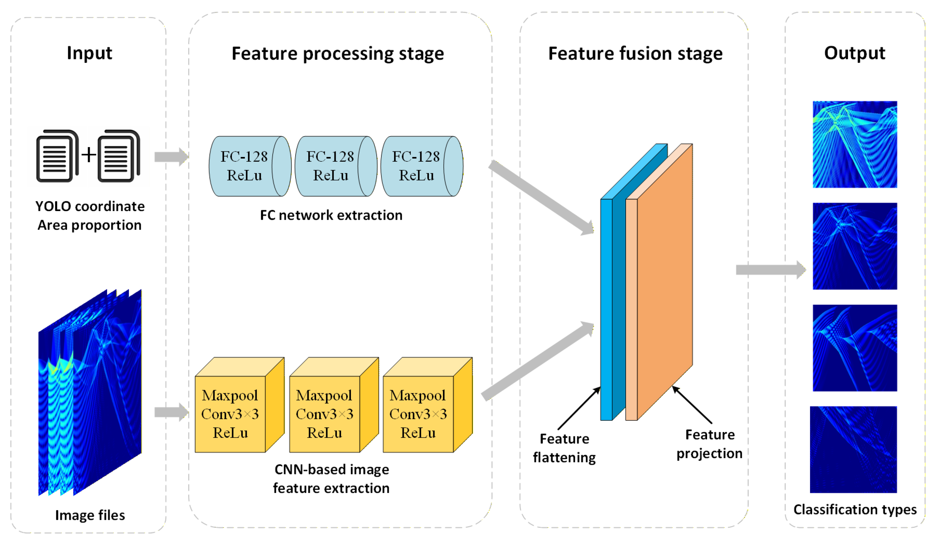
However, the original VGG16 network is typically designed for single-channel input when processing grayscale images, with its convolutional kernel parameters optimized based on a single data modality [44]. In the preceding phase, by improving the ResNet-34 network, regional segmentation results for raw images were obtained in the task of sound SZ and CZ segmentation. The output files include YOLO-format files for feature regions of sound TL images, as well as the area proportions of sound SZs and CZs. Therefore, when classifying preprocessed images, a dual-channel input design that combines visual features and geometric prior features should be adopted [45]. This dual-channel design achieves synergistic optimization of purely data-driven texture learning and prior-augmented learning by processing visual features and hand-crafted spatial features in parallel [46]. Specifically, the raw grayscale TL images are fed into the first channel, which preserves the spatial details of the sound field energy distribution; the extracted geometric prior parameters (including the area proportions and regional coordinates of sound SZs and CZs) are input into the second channel [47]. These regional coordinates are strictly encoded as bounding box corners. This compact rectangular representation effectively encapsulates the essential macro-scale physical spans (horizontal range and vertical depth) while smoothing out diffuse, noisy acoustic boundaries, thereby acting as a crucial geometric regularizer to prevent small-sample overfitting. The architecture of this improved dual-channel classification model is illustrated in Figure 5.

To achieve efficient fusion of such bimodal data, modifications to the front-end structure and feature interaction mechanism of the VGG16 network are required. First, a dual-branch parallel processing architecture is constructed at the input layer. For the visual feature branch, the standard convolutional modules of VGG16 can be retained to perform layer-by-layer spatial feature extraction on raw grayscale images, capturing local details such as sound field energy gradients and CZ edge morphology. For the geometric prior feature branch, spatial encoding is performed on the CZ area proportion parameters and the sound-ray-density gradient histogram. The area proportion scalar is converted into a $224\times 224$ full-resolution heatmap, where pixel values are positively correlated with the positions of CZs; meanwhile, the sound-ray-density gradient histogram is mapped to a $224\times 224$ feature map through fully connected layers, with bilinear interpolation used to achieve spatial dimension matching. These two components are superimposed to form a geometric prior feature map, which is then input into a lightweight convolutional module to extract global statistical features.

To integrate the vector characteristics of visual and geometric prior features in the dual-channel input, in the feature fusion stage, the model adopts a feature alignment strategy to unify the number of channels between the output of the 4th convolutional block in the visual branch and the output of the 3rd layer in the geometric feature branch. A $1\times 1$ convolution is used to increase the number of channels of the geometric prior features to 512, ensuring consistency in spatial resolution with the visual branch.

Finally, to address the overfitting issue caused by the excessive number of parameters in the fully connected layers of the traditional VGG16, the model replaces the fully connected layers with global average pooling (GAP): the three fully connected layers at the end of the original network are removed, and GAP is directly applied after feature fusion to reduce the feature map to a 512-dimensional vector. This operation effectively reduces the computational load of model parameters while preserving the global statistical information of spatial features.

The improved model embeds the geometric prior knowledge of the sound field into the deep learning framework through a dual-channel input architecture, solving the problem of disconnection between visual features and geometric parameters in traditional methods. The visual branch focuses on the microscopic representation of the local sound field energy distribution, while the geometric feature branch quantizes the morphological laws of CZs from a global perspective. The two branches achieve complementary enhancement through multi-scale concatenation and feature compression, improving the nonlinear expression ability of the network and achieving comprehensive improvements in both classification efficiency and accuracy.

Considering the specificity of the dual-channel input structure, the training procedure of the improved VGG16 network needs to take into account both the heterogeneous characteristics of multimodal data and the convergence stability of the model. In the data preprocessing stage, the heterogeneity of the dual-channel input requires differential processing of visual and geometric prior data. The input of the visual branch is the original sound TL grayscale image. Linear normalization is used to map the original sound intensity values to the interval $[0,1]$, and bicubic interpolation is adopted to uniformly scale the image to a resolution of $224\times 224$, so as to fully retain the spatial details of the sound field energy distribution [48]. The CZ area proportion parameters and sound-ray-density gradient histograms input to the geometric feature branch need to be converted into spatially encoded features: first, the area proportion parameters are used to generate a full-resolution heatmap, where the pixel values at the positions corresponding to the CZs are set to the proportion scalar values, and the pixel values of non-CZs are set to zero; subsequently, the 10-dimensional gradient histogram is expanded into a $224\times 224$ feature map through bilinear interpolation, which is then pixel-wise superimposed with the heatmap to form a geometric prior feature map; finally, normalization is performed to constrain the geometric prior feature map to the interval $[-1,1]$, so as to enhance the training stability of the model. The alignment processing of the dual-channel data ensures the effectiveness of subsequent feature fusion.

The initialization strategy of network parameters directly affects the convergence speed and generalization ability of the model. The visual branch inherits the pretrained VGG16 weights on the ImageNet dataset [49]; the lightweight convolutional layers of the geometric feature branch are initialized with a normal distribution to adapt to the nonlinear characteristics of the ReLU activation function; the weights of the feature encoding layer are initialized as an identity matrix to ensure the lossless transmission of geometric prior features. The $1\times 1$ convolutional layer of the fusion module is initialized with a Xavier uniform distribution to balance the weight allocation of dual-channel features [50]. Through the above-mentioned differential initialization strategy, the model can establish initial associations between multimodal features at the initial stage of training, laying a foundation for the convergence of subsequent training.

The design of the loss function aims to address the problems of class imbalance and consistency with geometric prior logic. A weighted cross-entropy loss function is adopted, which assigns higher weights to infrequent classes according to the class distribution in the training set, so as to alleviate prediction bias caused by sample imbalance. Meanwhile, a geometric constraint regularization term is introduced to force the model predictions to be logically consistent with geometric prior features. Specifically, the geometric constraint regularization term utilizes an indicator function that applies a linear penalty to the predicted probability of physically contradictory classes (e.g., predicting a low-proportion class when the input CZ area proportion exceeds 70%). Because the area proportion acts purely as a constant external condition during backpropagation, the gradient flows exclusively through the network’s continuous probability outputs, making the penalty strictly end-to-end differentiable.

The physical penalty term $L_{\mathrm{phy}}$ is formally defined as Equation (11):

$$L_{\mathrm{phy}}=\mathbb{I}(A_{\mathrm{CZ}}>0.7)·\sum _{c\in {\mathcal{C}}_{\mathrm{contra}}}{P}_{\mathrm{pred}}\left(c\right),$$

(11)

where $\mathbb{I}(·)$ is the indicator function (evaluating to 1 when the condition holds and 0 otherwise), $A_{\mathrm{CZ}}$ denotes the CZ area proportion provided by the Stage 1 segmentation output, ${\mathcal{C}}_{\mathrm{contra}}=\{\mathrm{Weak}\mathrm{Convergence},\mathrm{Shadow}\mathrm{Zone}\}$ is the set of physically contradictory classes for the high-proportion case, and $P_{\mathrm{pred}}\left(c\right)$ is the Softmax-predicted probability assigned to class c. Because $A_{\mathrm{CZ}}$ enters the penalty solely as a constant gating condition during backpropagation, gradients flow exclusively through the continuous Softmax outputs $P_{\mathrm{pred}}\left(c\right)$, ensuring strict end-to-end differentiability.

It should be noted that Equation (11) encodes only the high-proportion constraint direction ($A_{\mathrm{CZ}}>0.7\Rightarrow$ must be strong convergence). The symmetric low-proportion case ($A_{\mathrm{CZ}}<0.2\Rightarrow$ shadow zone) is deliberately not penalized, because in the 20–50% intermediate range—where the exploitable and weak convergence types are discriminated by spatial continuity rather than area proportion alone—a rigid low-proportion penalty would risk incorrectly suppressing valid weak convergence predictions. The penalty is therefore designed as a conservative, asymmetric safeguard: it intervenes only when the physical evidence is unambiguous (very high CZ proportion), and defers to the data-driven classifier in all other regimes.

The mathematical expression of the joint loss function is given as Equation (12):

$$L=\alpha L_{\mathrm{CE}}+\beta L_{\mathrm{phy}},$$

(12)

where $\alpha =0.8$ and $\beta =0.2$ are hyperparameters, and the optimal ratio is determined through grid search. As a fundamental physical safeguard rather than a tunable heuristic, this penalty qualitatively contributes to the framework by actively eliminating physically absurd misclassifications caused by severe localized noise.

A selective parameter freezing and joint fine-tuning strategy was adopted during training to balance the learning rates of the bimodal features and prevent the large initial gradients of the classification layer from disrupting the pretrained visual weights. The optimization process involved freezing the visual branch to concentrate on training the geometric feature encoding network and the classification layer, allowing them to establish initial discriminative capabilities. Subsequently, the visual network was unfrozen to perform end-to-end joint fine-tuning with a minimal learning rate, ensuring the perfect alignment of the feature extractors and the final decision boundary. A dynamic learning-rate-decay strategy was applied throughout the training process, with the learning rate decayed to half of its original value every ten epochs to achieve stable convergence. The training monitoring mechanism further ensured model stability by incorporating an early-stopping mechanism based on the real-time monitoring of the validation loss and accuracy, which automatically terminates the training process upon sustained performance stagnation. Furthermore, L2 norm clipping was performed on the gradients of the geometric feature branch to avoid gradient explosion caused by differences in feature dimensions.

2.4. Feature Enhancement Based on Convolutional Autoencoder

To address the practical challenge of acoustic data scarcity in unfamiliar maritime regions, where it is typically not feasible to acquire extensive in situ measurements, this study employs the geographically distinct South China Sea simulated dataset (500 images) as a controlled proxy for a data-scarce target domain, while the distribution discrepancy between the Northwest Pacific source domain and the South China Sea target domain (known as domain shift) motivates the adoption of a few-shot classification paradigm based on deep transfer learning in the third stage of the cascaded framework. This section proposes a few-shot sound field classification method based on pretrained transfer learning. Prior to the experiments, the adopted pretrained transfer learning strategy is determined and a hybrid sound field image enhancement method based on Mixup and convolutional autoencoder is proposed. This method effectively suppresses the overfitting phenomenon in the few-shot training process and improves the generalization ability of the sample dataset. During the transfer learning training process, the improved VGG16 model is pretrained on deep-sea sound field data of the Northwest Pacific Ocean, driven by temperature and salinity data from multiple sea areas. A parameter freezing strategy is used to retain the universal feature extraction capability, realizing domain adaptive transfer of multi-scale sound field features and completing the few-shot sound field classification task.

Mixup is an image augmentation technique based on linear interpolation that can enhance images of different categories [51,52]. Its core principle is to linearly mix training samples and their corresponding labels to generate new sound field data samples, thereby improving the classification accuracy of the model while enhancing its generalization ability, as calculated using Equation (13):

$$(x_n,y_n)=\lambda (x_i,y_i)+(1-\lambda )(x_j,y_j),$$

(13)

where $x_i$ and $y_i$, along with $x_j$ and $y_j$, are two randomly selected sound field image sample pairs; x denotes the TL matrix, y represents the corresponding sound field-type label, and $x_n$ and $y_n$ represent the new sample after mixing augmentation [53,54]. The mixing coefficient $\lambda \in [0,1]$ follows a Beta distribution. 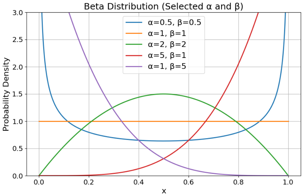To ensure that the mixed sound ray distribution conforms to the physical laws of sound propagation in sound SZs and CZs, the sampling range of the mixing coefficient $\lambda$ must be constrained to avoid excessive discrepancies between the augmented images and the actual TL images, thus preventing the periodic characteristics of sound propagation in CZs from being disrupted [55]. The probability density function plot of the Beta distribution is illustrated in Figure 6, where the value is affected by the interaction of $\alpha$ and $\beta$. 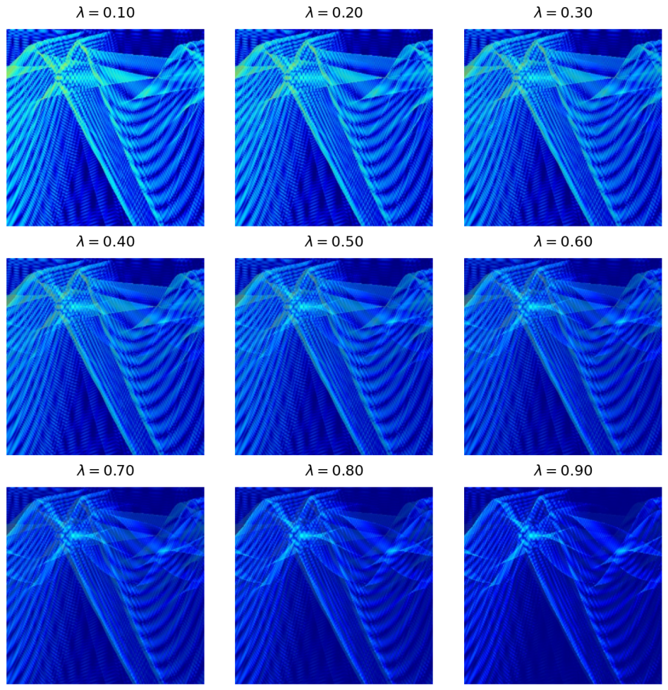A larger $\alpha$ leads to an increase in the training error of the Mixup augmentation method, which is reflected in the results as an increase in the mixing ratio of different images and an enhancement in generalization ability. The data augmentation results under an unfixed mixing coefficient are presented in Figure 7, where one typical SZ sound field feature and one typical CZ sound field feature are randomly selected for the Mixup operation, and nine augmented images with mixing effects are output.

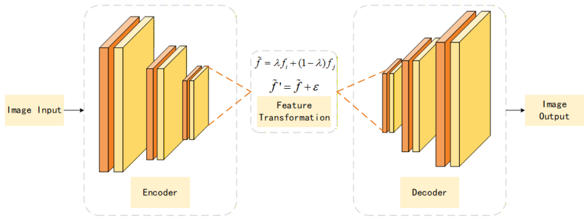
After mixing and augmenting two sound field region images using the Mixup method, the weights of the two images change with the mixing coefficient. The mixed and augmented images can serve as an expanded dataset to improve the training effect of the source-domain model. The convolutional autoencoder (CAE) is a classic deep learning architecture with prominent advantages in image feature learning and data augmentation. This method adopts CAE to enhance sound field images, where the encoder extracts sound ray propagation features from TL images, performs controllable transformations in the feature space, and finally reconstructs new samples conforming to sound field geometric and structural characteristics via the decoder [56,57]. Compared with traditional methods, CAE-based feature enhancement can automatically learn key patterns such as sound-ray-density distribution and CZ texture through convolutional operations and realize complex nonlinear interpolation in the feature space, which better meets the requirements of real-world datasets [58].

The image enhancement process consists of three steps:

• The original image is fed into the encoder to extract a 128-dimensional feature vector f, and the feature space distribution model of the training set is constructed.
• In the feature transformation step, feature vectors $f_i$ and $f_j$ from different samples are randomly selected for linear interpolation in the feature space, as shown in Equation (14):

  $$\tilde{f}=\lambda f_i+(1-\lambda )f_j,\lambda \sim \mathcal{U}(0.3,0.7)$$

  (14)
• Noise is added to the interpolated feature vector to improve the generalization ability of the TL image dataset, as defined in Equation (15):

  $${\tilde{f}}^{\prime }=\tilde{f}+\epsilon ,\epsilon \sim \mathcal{N}(0,0.1)$$

  (15)

In the image reconstruction stage, the transformed feature vector is fed into the decoder and the reconstructed sound field image is output, which preserves the sound ray distribution characteristics of the original image. The structure of this method is illustrated in Figure 8. The Mixup method is combined with the convolutional autoencoder-based image enhancement approach to achieve in-depth expansion of the details of image samples.

2.5. Ocean Sound Field Feature Classification Method Based on Transfer Learning

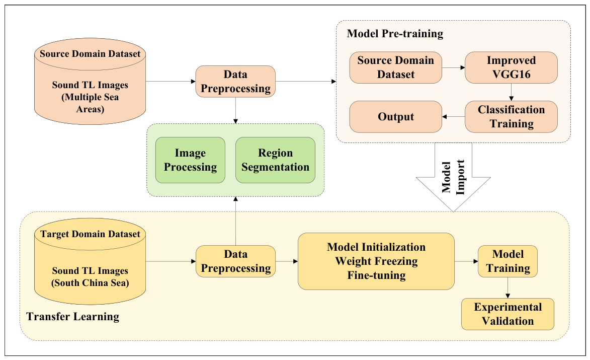
The flowchart of the few-shot sound field feature classification method based on pretrained transfer learning proposed in this section is shown in Figure 9. The algorithm consists of two main parts: the pretraining of the source-domain model and the training of the target-domain model after transfer learning. In the source-domain learning step, a large number of TL images are first obtained and the relationships between different types CZ ratios and CZ characteristics are constructed. Then, image-level preprocessing is performed, which is similar to the region segmentation in the improved ResNet-34 network mentioned earlier [59]. After grayscale processing and average calculation of grayscale regions, the proportions of sound SZs and CZs are extracted and fed into the improved VGG16 network of the source domain as geometric prior features for model pretraining. After outputting the recognition results, verification and feedback are conducted to further confirm the feasibility of the source-domain model in recognition and classification.

In the target-domain training step, similar data preprocessing is first implemented on the few-shot target-domain dataset [60]. Then, transfer learning is used to import the source-domain model, the low-layer parameters of the source-domain model are frozen, and the high-layer parameters are fine-tuned to obtain a network model suitable for the target domain. Finally, a well-trained model for few-shot TL images is obtained through training and validation [42,61].

The weighted cross-entropy loss function is adopted to address the class imbalance between the target-domain dataset and the source domain, which is formulated as Equation (16):

$$L_{cls}=-{\displaystyle \sum _{i=1}^N}{\omega }_i·y_{i}log\left({\widehat{y}}_i\right),$$

(16)

where $y_i$ is the target class label, ${\widehat{y}}_i$ is the predicted probability, and ${\omega }_i$ is the class weight, which can be adjusted appropriately according to the sample proportion of each class in the target domain. In practice, the class weights are set to 0.8 (CZ-S), 1.2 (CZ-E), 1.5 (CZ-W), and 0.8 (SZ), with higher weights assigned to the minority and easily confused classes to mitigate class imbalance. These values are configurable in the released source code. Meanwhile, to reduce the overfitting risk of the model, the regularization loss of the model is calculated using Equation (17):

$$L_{reg}=\lambda {\displaystyle \sum _{j=1}^M}{\theta }_j^2,$$

(17)

where $\lambda$ is the regularization coefficient and ${\theta }_j$ denotes the model parameters.

To quickly adapt to the class space of the target domain during the classification layer training step, the AdamW optimizer is selected, while backbone parameters are frozen to enhance the generalization ability of the model. The initial learning rate is set to $1\times {10}^{-4}$ and the batch size is set to 16. A cosine annealing learning rate schedule is adopted to dynamically adjust the learning rate and accelerate the network convergence, as expressed in Equation (18):

$${\eta }_t={\eta }_{\min }+{\displaystyle \frac{1}{2}}\left({\eta }_{\max }-{\eta }_{\min }\right)\left(1+cos\left({\displaystyle \frac{t}{T}}\pi \right)\right),$$

(18)

where the maximum learning rate is ${\eta }_{\max }=1\times {10}^{-4}$, the minimum learning rate is ${\eta }_{\min }=1\times {10}^{-5}$, and the cycle length is $T=50$.

The hierarchical training process is executed in three sequential phases. Initially, for class space adaptation, all convolutional layers are frozen and only the fully connected layers are trained. Operating with a learning rate of $1\times {10}^{-5}$ for 5 epochs, this phase quickly adapts the network to the class space of the target domain and establishes an initial classification boundary. Subsequently, to achieve feature fine-tuning and fine-grained adjustment, the final six convolutional layers are unfrozen, allowing the fully connected layers and convolutional classification layers to be jointly trained. Utilizing a learning rate of $1\times {10}^{-4}$ coupled with a cosine annealing schedule, the model is trained for 20 epochs. This stage realizes the fine-grained feature recognition of target-domain data and aligns the feature tuning with the source-domain model. Finally, for global representation alignment, the global statistical module is jointly fine-tuned. The learning rate is maintained at $1\times {10}^{-5}$ for an additional 15 epochs to further enhance the feature classification capability, specifically for the South China Sea sound TL images, thereby completing the comprehensive cross-domain adaptation protocol.

3. Results and Analysis

3.1. Performance of Sound Field Region Segmentation

Image-based discrimination methods segment acoustic SZs and CZs from high-resolution sound TL images generated by the Bellhop model by combining grayscale differences and internal consistency. Unlike standard computer vision tasks, acoustic CZs and SZs do not possess rigid, pixel-level geometric boundaries. Due to the inherent continuous refractive nature of ocean waveguides and Gaussian beam propagation [8,62], acoustic energy diffuses smoothly. Consequently, while metrics such as intersection over union (IoU), Dice coefficient, precision, recall, and F1-score are widely accepted for comprehensive evaluation in conventional semantic segmentation, evaluating the network on these strictly geometric intersection metrics against artificially thresholded pseudo-labels would impose arbitrary rigid boundaries that fundamentally violate physical reality. Therefore, rather than relying on absolute physical boundary labels, an unsupervised evaluation index is designed to verify the correctness of the segmented regions based on predefined grayscale-value distributions. This approach ensures the model directly evaluates the disparity of acoustic energy concentration. To intuitively reflect the segmentation performance, regional grayscale contrast and intra-region consistency are adopted. Equation (19) defines the degree of grayscale difference between acoustic SZs and CZs:

$$CR={\displaystyle \frac{{\mu }_{con}-{\mu }_{aco}}{{\mu }_{con}+{\mu }_{aco}}}\times 100\%,$$

(19)

where ${\mu }_{aco}$ and ${\mu }_{con}$ represent the average grayscale values of the regions classified as acoustic SZs and CZs, respectively. A larger contrast value indicates a more significant grayscale difference and a reasonable segmentation result, while a lower value represents region confusion. Furthermore, the internal consistency of the regions must be evaluated, where Equation (20) measures the uniformity of grayscale values within a single class region:

$$IR{C}_{aco}=1-{\displaystyle \frac{{\sigma }_{aco}}{\sigma }},IR{C}_{con}=1-{\displaystyle \frac{{\sigma }_{con}}{\sigma }},$$

(20)

where ${\sigma }_{aco}$ and ${\sigma }_{con}$ represent the grayscale variances of the acoustic SZs and CZs and $\sigma$ represents the global variance. By evaluating this consistency index it is possible to determine whether noise or mis-segmentation occurs. Ultimately, this unsupervised statistical system comprehensively reflects the model segmentation capability and provides a reliable accuracy criterion for optimizing the region segmentation method in subsequent experiments.

After making specific modifications to different residual blocks of the ResNet-34 network, comparative experiments are designed to verify whether the segmentation method based on the improved ResNet-34 network can stably extract the proportion characteristics of CZs and acoustic SZs, thereby providing stable inputs for subsequent sound field feature image classification. The key evaluation metric is set as the accuracy of acoustic SZs and CZs on the same dataset. The experimental environment configuration utilizes an NVIDIA RTX 3060 GPU as the hardware platform and PyTorch 1.12.1 as the software framework. To avoid overfitting, an early-stopping strategy is adopted during training and the maximum number of training epochs is limited to 100. A comparative analysis was conducted between four approaches, including threshold-based region growing using the original ResNet-34 architecture and the improved ResNet-34 architecture. The differences in the regional segmentation strategies of each method are summarized in

Table 2. Regional segmentation strategies of the compared methods.

Comparison Method	Regional Segmentation Strategy
Threshold segmentation method	Calculate the sound ray density threshold based on the Otsu algorithm and statistically analyze the regional area proportion according to the threshold.
Region-growing method	Select initial seed points and expand to the entire convergence zone region using local similarity.
Original ResNet-34 network	Extract multi-scale features through residual blocks and output the multidimensional vector after global average pooling.
Improved ResNet-34 network	On the basis of the original ResNet-34 network, combine a global statistics module and an adaptive loss function to output the area proportion of the convergence zone.

.

To verify the effectiveness of the proposed architectural enhancements and the joint loss function, comparative experiments were conducted using four methods: the traditional Otsu thresholding, the region-growing method, the original ResNet-34, and the improved ResNet-34 framework. The sound TL images, processed from temperature and salinity data in the Northwest Pacific Ocean, were used as input samples. To ensure fair comparison, the deep learning methods adopted identical training strategies. It should be explicitly clarified that the “Original ResNet-34” evaluated here represents a standard fully convolutional network (FCN) baseline, constructed with a ResNet-34 classification backbone and a basic bilinear upsampling prediction head, stripped of our proposed modifications. The experimental results of the regional segmentation are presented in

Table 3. Performance comparison of different methods.

Classification Method	Regional Gray Contrast (%)	Intra-Region Consistency
Traditional threshold method (Otsu)	63.5	0.72
Region-growing method	61.2	0.91
Original ResNet-34 (FCN Baseline)	74.2	0.84
Improved ResNet-34	86.9	0.89

.

Traditional image processing methods exhibit obvious limitations when dealing with continuous acoustic energy fields. The Otsu method relies on a single global threshold, leading to significant boundary estimation errors in regions with gentle density gradients. An excessively high threshold misclassifies fragmented CZs as acoustic SZs, while a low threshold fails to identify SZs effectively. Coupled with its susceptibility to background noise, the Otsu method yields a low regional gray contrast of 63.5% and an intra-region consistency of 0.72. Similarly, while the region-growing method automates seed point selection, it severely suffers from seed deviation in complex sound fields. A single seed point cannot cover multiple disconnected CZs, and complex boundary textures cause inaccurate growth, yielding an even lower regional gray contrast of 61.2%.

Compared to traditional algorithms, deep learning approaches demonstrate significant advantages. The canonical FCN baseline (Original ResNet-34) achieves a regional gray contrast of 74.2% and an intra-region consistency of 0.84. However, its standard architecture primarily focuses on extracting local texture features. Without targeted macro-level constraints, it inevitably loses critical global density distribution information during downsampling, making it difficult to establish an accurate physical feature distribution pattern.

The improved ResNet-34 overcomes these limitations by integrating the global statistical module and the lightweight FCN segmentation head, which extract and retain multi-scale spatial boundaries and macro-level statistical features. Critically, the proposed joint optimization strategy—combining the global area matching loss and the density gradient loss—is implemented. This mathematically constrains the global distribution patterns and effectively suppresses the risk of low-pressure pixel over-segmentation. Consequently, the improved network achieves the highest regional gray contrast of 86.9% and an excellent intra-region consistency of 0.89. This empirical comparison securely validates that the proposed physics-prior-augmented design effectively addresses the bottlenecks of purely data-driven models, ensuring high reliability for subsequent sound field feature classification.

However, this significant improvement in segmentation accuracy comes with a computational trade-off. As evaluated on the aforementioned NVIDIA RTX 3060 GPU platform, the integration of the global statistical module and the multi-branch spatial concatenation architecture inherently increases the model’s computational complexity. Specifically, under the same experimental conditions, with a batch size of 32 and an initial learning rate of $1\times {10}^{-5}$, the improved ResNet-34 boosts the regional gray contrast from 74.2% to 86.9% compared to the original ResNet-34; however, its training time correspondingly increases from 33 min to 55 min. Consequently, the improved model exhibits a higher inference latency compared to the canonical FCN baseline. Given that practical marine sonar applications often emphasize strict real-time processing capabilities, the computational efficiency of the current framework has not yet been fully optimized for edge-device deployment. Future research will explicitly focus on this aspect by employing model lightweighting techniques, such as network pruning and tensor optimization, to reduce the computational overhead, thereby enhancing the deployment feasibility while maintaining high segmentation reliability.

3.2. Evaluation of Dual-Channel Classification Model

To verify the superiority of the proposed method and obtain reliable sound field feature classification results, four groups of comparative experiments are designed in this section. The K-Nearest Neighbor algorithm, the random forest algorithm, the original VGG16 model, and the improved VGG16 model are adopted for comparative research. To strictly decouple the structural contribution of our dual-channel fusion mechanism, highly optimized modern heavy backbones were intentionally excluded from the baselines. This experimental control ensures that any performance gains are driven by the bimodal fusion mechanism itself rather than being artificially inflated by the massive data-fitting capacity of over-parameterized models. The experiments take the YOLO coordinate data, the region proportion data output by region segmentation in the first step, and the original sound TL images as inputs to complete the sound field feature classification. To ensure the fairness and reliability of the experiments, both the original VGG16 and the improved VGG16 models use the same training strategy.

In the classification task, the K-Nearest Neighbor algorithm discriminates samples by calculating the feature distance between test and training data, focusing on area proportion and spatial distribution characteristics. It determines the category through a voting mechanism among the K nearest neighbors, where measuring only effective features and tuning the parameter K mitigates invalid interference and improves high-dimensional accuracy. Alternatively, the random forest algorithm is an ensemble learning method that constructs multiple decision trees trained on randomly sampled feature subsets, outputting the final result through multi-tree voting fusion. It effectively integrates CZ proportions and spatial features for classification modeling. Furthermore, adjusting the number of trees and subset sizes optimizes classification performance while its ability to output feature importance rankings provides quantitative theoretical support for subsequent model optimization.

For the classification task of sound SZs and CZs, the original VGG16 network takes preprocessed sound TL images and their corresponding CZ proportion features as inputs. During the training phase the backpropagation algorithm is employed to optimize the network parameters by minimizing the cross-entropy loss function. Meanwhile, the resolution of input images affects the total number of network parameters to a certain extent, which in turn impacts the training time and classification accuracy of the model. To ensure the training effect and explore the influence of resolution on model performance, this section designs a comparative experiment on resolution. By adjusting the structure of the fully connected layers, the model is adapted to accept image inputs with four resolutions, including $32\times 32$, $64\times 64$, $128\times 128$, and $224\times 224$, to verify whether reducing the input resolution can effectively shorten the training time while maintaining classification accuracy. The experiments uniformly adopt the default multi-class cross-entropy loss function with a batch size of 16 an initial learning rate of $1\times {10}^{-5}$ and 100 training epochs. The experimental results are presented in

Table 4. Accuracy and training time under different resolutions.

Resolution Size	Accuracy/%	Training Time/min
$32\times 32$	27.31	35
$64\times 64$	44.16	47
$128\times 128$	68.17	102
$224\times 224$	79.34	366

.

Due to the abundance of edge details in sound SZ and CZ images, images with resolutions lower than $224\times 224$ cannot fully reflect the variation in grayscale values in the network, making it difficult to achieve satisfactory classification accuracy. Therefore, in the experiments on the VGG16 network model, the standard input resolution of $224\times 224$ is adopted to ensure the reliability of the subsequent experimental results.

Before conducting multi-method comparative experiments to verify the superiority of the improved VGG16 over the original network model in the classification task of sound SZs and CZs, it is necessary to first compare their training processes under the same dataset and initial condition settings. The training loss function is a key indicator in the model optimization process, reflecting the fitting ability of the model during the training and validation phases on the dataset, while the test loss function reflects the generalization ability of the model on unseen data. By comparing the function curves of the training loss and test loss of the two methods, the convergence speed stability and training performance of the improved design can be evaluated intuitively.

Figure 10 presents the comparison curves of training loss and test loss between the improved VGG16 network model and the original network model, where the blue curve represents the loss of the original VGG16 network model and the red curve represents the loss of the improved model. It can be clearly observed from the training loss comparison plot in the left panel of Figure 10 that the training convergence speed of the improved model is significantly faster than that of the original network model. Meanwhile, the final training loss value of the improved VGG16 is also lower than that of the original VGG16 network model, indicating that the improved method has better fitting ability on the training dataset. From the test loss comparison plot in the right panel of Figure 10 it can be seen that in the test set validation the test loss of the improved VGG16 also exhibits faster convergence speed and a lower final loss value. The final test loss of the improved model is reduced by more than 50% compared with the original model, demonstrating that the improved method has better generalization ability on the test dataset.

Through the comparison of loss function results, the effectiveness of the dual-channel input can be verified. By fusing visual features and quantitative features the improved method can optimize model parameters more efficiently and enhance generalization ability. In addition, it provides sufficient theoretical basis for subsequent accuracy comparison, further proving the superiority of the improved method in the classification task of sound SZs and CZs.

After loss function comparison experiments of the improved method, classification accuracy comparisons were performed for the K-Nearest Neighbor algorithm, the random forest algorithm, the original VGG16, and the improved VGG16 model. The accuracies for sound shadow and CZ classification in TL images are shown in

Table 5. Performance comparison of different classification methods.

Classification Method	Classification Accuracy/%
K-Nearest Neighbor algorithm	64.75
Random forest sound field feature classification method	81.28
Original VGG16 network model	82.34
Improved VGG16 network model	89.91

and Figure 11.

The K-Nearest Neighbor algorithm classifies sound TL images by calculating feature distances. It achieves relatively high accuracy in strongly convergent zones and sound SZs due to distinct feature differences but is prone to misjudgment caused by noise. In exploitable convergent zones and weakly convergent zones, the classification accuracy drops significantly to 51.8% and 54.4%, respectively, failing to meet task requirements, due to complex region boundaries and amplified noise interference. Although simple in implementation, the K-Nearest Neighbor algorithm is limited by feature dimensions and data distribution, making it unable to capture global statistical features of sound TL images and thus unreliable for sound field classification.

The random forest algorithm improves classification performance by integrating multiple decision trees, taking the proportion and coordinates of sound SZs and CZs as spatial features. It exhibits certain resistance to overfitting, with less classification loss from noise than the K-Nearest Neighbor algorithm. However, it still struggles with boundary textures, achieving only 65.0% and 68.3% accuracy for exploitable and weakly convergent zones, which falls short of the experimental goals. It is limited by computational resources: increasing decision trees and feature subsets leads to higher costs and higher probability of voting confusion, resulting in insufficient efficiency and accuracy.

The original VGG16 network extracts spatial features through convolutional layers and outputs classification results via fully connected layers. Despite good performance on natural images, pretrained on ImageNet its convolutional kernel parameters fail to effectively fuse region coordinates and area proportion information of simulated sound field images, relying only on texture-level recognition. This structural limitation is directly reflected in its overall classification accuracy of 82.34%. While it achieves relatively high accuracies of 90.6% and 87.9% in strongly convergent zones and SZs, respectively, due to their distinct textural features, its performance drops significantly in more ambiguous transitional areas. Specifically, it only reaches 74.1% and 76.3% accuracy in exploitable and weakly convergent zones, respectively. Lacking the ability to capture global statistical features it has obvious generalization bottlenecks and is only suitable as a control group for performance comparison.

The improved VGG16 network adopts a dual-channel input design, where the visual channel focuses on local feature distribution while the geometric prior channel quantifies global region proportion, achieving complementary enhancement through feature concatenation. Meanwhile GAP is used to replace fully connected layers, reducing the number of parameters and improving computational efficiency. This architectural advantage translates into a superior overall classification accuracy of 89.91%. The dual-channel fusion particularly excels in complex regions, raising the recognition accuracy for exploitable and weakly convergent zones to 80.9% and 83.3%, respectively, which effectively overcomes the recognition bottlenecks of the original model. Furthermore, it achieves near-perfect recognition in strongly convergent zones and SZs, with accuracies reaching 98.9% and 95.9%, respectively. The experimental results demonstrate that the improved VGG16 network comprehensively outperforms all the traditional methods and the original network, enabling accurate and efficient classification of sound field feature regions.

3.3. Generalization Validation Under Data-Scarce Scenarios

Before detailing the experiments, it is crucial to clarify the substantial domain shift between the simulated source domain (Northwest Pacific Ocean) and the simulated target domain (South China Sea). Oceanographically, compared to the deep and stable Northwest Pacific, the South China Sea exhibits distinctively different bathymetry (e.g., much shallower mean depths and complex continental slopes), varied sound-speed profile (SSP) characteristics (e.g., warmer upper layers and shallower mixed layers), and highly active mesoscale eddy phenomena. These pronounced environmental disparities lead to marked spatial shifts and morphological variations in the acoustic fields, preventing standard machine learning models from generalizing directly. However, the proposed transfer learning strategy does not rely on the statistical similarity of the raw physical parameters (such as PCA distributions of SSPs) between the two basins. Instead, by processing transmission loss (TL) images, the network transfers the universal visual–geometric representations of wave propagation physics (e.g., refractive caustics and multipath interference boundaries) that remain topologically consistent across different oceans. This fundamental mechanism allows the model to successfully bridge the substantial macroscopic gap and provides robust cross-domain interpretability.

The comparative experiments in this section consist of three interconnected parts designed to validate this cross-domain generalization under data-scarce scenarios. First, the model trained with the augmented dataset is compared against the one trained without augmentation to verify the performance improvement yielded by the augmentation strategy. Second, the training performance between the source domain and the target domain is evaluated to prove the applicability of the transfer learning method for sound field region feature classification. Finally, the classification accuracy of the standard improved VGG16 model is compared with the optimized model trained via transfer learning to demonstrate that the proposed method is significantly more suitable for few-shot classification tasks than neural network models, lacking pretraining and transfer learning. To evaluate these strategies, images augmented by a Mixup–convolutional autoencoder hybrid method were utilized to train the transfer learning-based improved VGG16 model and the results were compared against baseline datasets, including non-augmented and exclusively Mixup-augmented variants. The resulting model accuracy for each method is presented in

Table 6. Model accuracy of different methods with data augmentation.

Dataset	Classification Accuracy/%
Mixup–convolutional autoencoder	91.28
Mixup	90.74
Original dataset	87.34

.

As shown in Table 6, the Mixup–CAE hybrid method (91.28%) and the Mixup-only baseline (90.74%) yield comparable classification accuracies, with the 0.54-percentage-point difference falling within the expected variance of single-run results. Given that multi-run statistics with error bars are not available under current computational constraints, this marginal numerical gap should not be interpreted as a statistically meaningful accuracy gain attributable to the CAE module. The model performance curves of the three datasets are presented in Figure 12, Figure 13 and Figure 14.

By cross-referencing the model performance curves in Figure 12, Figure 13 and Figure 14 with the quantitative results in Table 6, the impact of different data augmentation strategies on model training dynamics can be systematically evaluated. When utilizing the unaugmented original dataset, a distinct divergence between the training and test accuracy curves is observed, indicating an overfitting tendency, where the model generalization capacity is constrained, resulting in a baseline classification accuracy of 87.34%. The application of the Mixup augmentation strategy reduces this generalization gap, restricting the curve divergence and improving the overall classification accuracy to 90.74%. Furthermore, the hybrid image augmentation method integrating Mixup and the convolutional autoencoder yields substantially enhanced convergence stability compared to both the Mixup-only and the original dataset baselines. The corresponding performance curves exhibit a markedly higher degree of consistency between training and test metrics throughout the epochs, with visibly reduced loss oscillation and a narrowed generalization gap, demonstrating that the overfitting phenomenon is effectively suppressed. Rather than providing a statistically significant accuracy margin over Mixup-only augmentation, the primary contribution of the CAE module lies in its structural regularization effect: by operating in the latent feature space, the CAE enforces smoother and more physically plausible sample interpolations, which stabilizes the training dynamics and yields more consistent convergence trajectories across epochs. The observed classification accuracy reaches 91.28%. These comparative results indicate that the proposed hybrid data augmentation method provides a robust mechanism to prevent the network from merely memorizing training samples, thereby improving training stability and generalization reliability under data-scarce conditions.

Figure 15 presents the accuracy and loss curves of the source-domain model evaluated on the training and test sets during the initial training phase. Observing the loss evaluation trends, the values consistently decrease and eventually stabilize, indicating that the model has reached an optimal convergence state. Correspondingly, the accuracy metrics exhibit a significant upward trajectory before maintaining a stable plateau. Notably, the minimal divergence between the training and test curves reflects the distinct advantage of abundant source data, which enables the network to learn highly generalizable underlying features without exhibiting overfitting tendencies. This robust convergence behavior confirms that the source-domain model can effectively extract and classify acoustic ray features, providing a reliable foundational weight configuration for subsequent transfer learning tasks.

The verified sound field classification model from the source domain is subsequently transferred to the target domain, where it undergoes a fine-tuning process with frozen weights to adapt to the small-sample South China Sea dataset. Figure 16 delineates the convergence behavior and generalization trends of the target-domain model. Compared to the source-domain training, a slightly wider generalization gap between the training and test curves emerges, which accurately reflects the inherent domain shift and the expected overfitting risks associated with data scarcity. However, despite this structural divergence the overall loss and accuracy curves maintain stable convergence trends, demonstrating high relative performance. These experimental results theoretically and empirically prove that the source-to-target transfer learning strategy effectively leverages pretrained weights to mitigate the limitations of small sample sizes, thereby successfully addressing the sound field region feature classification problem under restricted data conditions.

To test the performance of the improved VGG16 network and the effectiveness of pretrained transfer learning under few-shot conditions, an improved VGG16 network untrained on source datasets was tested on 200 South China Sea sound TL images alongside comparisons to the transfer learning method. The overall performance results are presented in

Table 7. Comparison of overall classification accuracy between different algorithms.

Classification Method	Classification Accuracy/%
Improved VGG16 network model	42.60
Improved model based on transfer learning	84.45

and category specific recognition accuracies are illustrated in Figure 17.

It should be explicitly noted that the two rows in Table 7 differ in three respects simultaneously: the 42.60% baseline employs (i) no source-domain pretrained weights (trained from scratch on 200 target-domain samples only), (ii) no Stage 1 geometric prior features (single-channel input), and (iii) no Mixup–CAE data augmentation (original unaugmented data), whereas the 84.45% model incorporates all three interventions. The 41.85-percentage-point gap therefore represents the combined synergistic effect of transfer learning, geometric priors, and hybrid data augmentation operating in concert, rather than the isolated contribution of transfer learning alone.

According to the experimental results, while the improved VGG16 network demonstrates high applicability within the homogeneous source domain, its performance collapses catastrophically when directly applied to the few-shot target domain without any of the three enabling mechanisms—source-domain pretrained weights, Stage 1 geometric priors, and Mixup–CAE data augmentation. The 42.60% accuracy, merely 17.6 percentage points above the 25% random chance baseline for four-class classification, confirms that a deep network trained from scratch on only 200 target-domain samples, deprived of all three mechanisms, is fundamentally unable to learn meaningful acoustic features.

Nevertheless, the relative magnitudes of the three factors can be approximately calibrated using the source-domain component-wise experiments. In the source domain, the geometric prior channel independently contributes approximately 7.6 percentage points (Table 5: 89.91% dual-channel vs. 82.34% single-channel VGG16), and the Mixup–CAE augmentation independently contributes approximately 3.9 percentage points (Table 6: 91.28% vs. 87.34%). Even under the conservative assumption that both contributions are fully additive and transferable to the target domain, the remaining gap—on the order of 30 percentage points—must be attributed to transfer learning. This dominance is consistent with the qualitatively distinct role of pretrained weights: data augmentation and geometric priors enrich the input information available to the model, but transfer learning provides the essential weight initialization that makes gradient-based learning feasible at all under extreme data scarcity. The source-domain pretrained weights encode universal acoustic propagation patterns—refractive caustics, multipath interference boundaries, and periodic convergence zone structures—that are topologically conserved across ocean basins and serve as an indispensable inductive starting point for target-domain adaptation.

To address this generalization bottleneck, this research fundamentally modifies the feature extraction paradigm. A hybrid data augmentation method combining Mixup and a convolutional autoencoder is introduced to enhance the extraction of local sound field features. Simultaneously, a pretrained transfer learning strategy is implemented to migrate global feature representations from the source domain to the target domain. This dual enhancement improves the adaptability of the model to small-sample conditions, enabling the optimized target model to achieve a stable overall classification accuracy of 84.45%. By analyzing the specific classification performance across the four acoustic categories, it becomes evident that the underlying morphological characteristics of the sound field directly correlate with the recognition accuracy. The model demonstrates effective capability in identifying strong CZs and SZs, achieving accuracies of 93.1% and 87.2%, respectively. This outcome is primarily due to the distinct macro-visual features and high gray value contrasts inherent to these regions, which correspond with the global semantic extraction capabilities reinforced by the transferred weights. Conversely, exploitable convergence and weak CZs inherently possess gentler density gradients and ambiguous regional boundaries, making them traditionally challenging to isolate. However, driven by the local feature enhancement of the hybrid augmentation strategy, the proposed model mitigates this bottleneck, lifting the recognition accuracies for exploitable and weak CZs to 77.6% and 79.9%, respectively. Consequently, these results validate that the synergy among transfer learning, geometric priors, and hybrid data augmentation allows the network to accurately capture both macro-level distributions and micro-level boundaries, making it uniquely equipped to handle the complexities of sound field classification under severe data constraints.

4. Discussion

The identification of acoustic SZs and CZs provides critical support for ocean exploration. Traditional methods primarily rely on statistical data analysis, which only estimates occurrence probabilities and struggles to provide accurate regional detection schemes. Conversely, conventional CNNs often exhibit low classification accuracy due to the lack of specialized adaptation to sound-ray propagation characteristics. This study transitions from traditional probability estimation to precise region identification by introducing a data-driven framework optimized for acoustic image features. According to the current canonical taxonomy of physics integration in scientific machine learning [46,63], our methodology is strictly positioned as physics-prior-augmented deep learning. Rather than embedding physics-informed loss functions (such as partial differential equation residuals) or employing physics-encoded architectures, physical principles are incorporated into our framework exclusively as priors. These physics priors enter the system through two specific channels: the robust Bellhop-generated training dataset, and the hand-crafted geometric priors derived post hoc from the Stage 1 segmentation outputs. By leveraging targeted structural network improvements alongside these physical priors, the proposed framework successfully achieves accurate acoustic region segmentation and classification without incurring the extensive computational overhead of solving complex acoustic PDEs.

Positioning the proposed framework among these recent advances reveals several instructive methodological contrasts. First, unlike the Transformer-based CGF-Unet [23], which relies on self-attention for global context modeling, our lightweight ResNet-34 with multi-scale spatial concatenation at the bottleneck and global statistical pooling achieves effective global perception while preserving the inductive bias of convolutions—a critical regularizer given our moderate dataset size of 5000 images. Second, whereas the contrastive few-shot framework of Cui et al. [24] operates on 1D acoustic spectra with metric-learning objectives, our pipeline processes 2D TL images and explicitly couples Mixup-based augmentation with convolutional autoencoder feature enhancement, directly mitigating the overfitting risks inherent to high-dimensional image data under few-shot constraints. Third, in contrast to the fully physics-informed approach of Chen et al. [26], which enforces PDE residuals in the loss function, our physics-prior-augmented strategy, injecting physical knowledge exclusively through the Bellhop-generated training dataset and post hoc geometric features, achieves a more favorable accuracy-to-computational cost trade-off for the targeted CZ/SZ classification task, where pointwise sound-pressure fidelity is unnecessary. Finally, the cross-domain protocol of Mohammadi et al. [25] shares our finding that ImageNet-pretrained CNNs provide viable initial representations for acoustic tasks; our framework extends this principle by inserting an intermediate source-domain pretraining stage before target-domain fine-tuning (South China Sea), which we find critical for bridging the larger domain gap between geographically distinct ocean environments.

The proposed framework addresses the difficulty of extracting features from complex deep-sea acoustic fields through an improved ResNet-34 segmentation method. By incorporating deformable convolutions and a global statistical module, the network adapts to the unique spatial distribution of acoustic TL. Compared to traditional threshold methods—which typically plateau at lower accuracy limits in complex environments—this approach provides a measurable improvement in regional target extraction and resolves the spatial ambiguity inherent to traditional depth excess calculations. Building upon these segmentation outputs an improved VGG16 network with a dual-channel input was developed to resolve the classification bottleneck caused by similar visual features in different acoustic regions. While conventional algorithms struggle significantly with easily confused transitional zones, jointly processing quantified area proportion features and raw visual features enables the dual-channel model to effectively capture the underlying patterns of sound TL images, vastly outperforming traditional baselines in discrimination tasks.

It is worth noting that the experimental design in Section 3 already provides systematic component-wise evidence regarding the contribution of each major architectural element. Specifically, the four-way comparison in Stage 1 (Table 3) isolates the combined effect of deformable convolution, the global statistical module, and the joint loss function versus the unmodified FCN baseline; the four-way classifier comparison in Stage 2 quantifies the gain attributable to the dual-channel fusion mechanism and the geometric prior branch; and the controlled augmentation variants in Stage 3 separately evaluate the contributions of Mixup and the convolutional autoencoder; while the transfer learning comparison (Table 7) measures the combined effect of all three interventions—pretrained weights, geometric priors, and data augmentation—acting in concert, with the source-domain component-wise calibrations providing approximate bounds on the individual contributions. In particular, the cross-domain comparison in Table 7 conflates three interventions; a controlled factorial experiment that isolates transfer learning from geometric priors and data augmentation in the target-domain setting—e.g., by holding two factors constant while varying the third—would provide a more granular attribution of the 41.85-percentage-point improvement and constitutes a specific priority for follow-up investigation. While these comparisons collectively demonstrate that each component contributes meaningfully to the final performance, a finer-grained per-component leave-one-out ablation across all six modules would require a combinatorially large number of controlled retraining runs with independent hyperparameter tuning for each configuration, which lies beyond the computational scope of the present study and is acknowledged as a direction for future investigation.

A primary challenge in practical underwater acoustics is the scarcity of in situ measured sound field data, which severely constrains the training of deep classification models. To systematically investigate this challenge under controlled and reproducible conditions, this study employs geographically distinct WOA18-simulated domains as a principled proxy—using abundant Northwest Pacific data for source-domain pretraining and a deliberately restricted South China Sea dataset to emulate the data-scarce target scenario. To resolve this limitation, a few-shot sound field feature classification method based on pretrained transfer learning was implemented. By training a source-domain model on abundant simulated data and subsequently applying frozen convolutional layers and fine-tuning to a target domain with limited samples, the network successfully migrated its classification capabilities. Unlike prior studies that either rely on massive in situ datasets or fail to generalize under severe domain shifts, this experimental design demonstrates that cross-domain transfer learning between geographically distinct acoustic environments, using a data-rich simulated source domain and a data-scarce simulated target domain as a controlled proxy for real-world conditions, provides a viable and reproducible pathway for acoustic classification under restricted data conditions, while acknowledging that ultimate validation against real at-sea measurements remains a necessary future step.

Despite the validated improvements in feature extraction and classification, several limitations regarding environmental complexity must be addressed in future research. The sound TL images utilized in this study were generated using temperature and salinity data synthesized from WOA18 climatological reanalysis datasets, which inherently harbor deviations from the actual dynamic marine environment. Real-world acoustic characteristics are subjected to complex superpositions of various ocean phenomena. Future studies should consider coupling multi-physics models and utilizing real-time data assimilation technologies to reduce the bias between reanalysis data and true environmental conditions. Furthermore, to maintain image uniformity and dataset completeness the current simulations did not account for the influence of complex seabed topography and bottom sediment types on acoustic reflection. In practical propagation scenarios, geological variations and transitional seabed layers exert complex effects on sound waves. Subsequent research must integrate high-resolution bathymetry data and acoustic parameter inversion techniques to quantify the reflection effects of different sediment types and develop sound field correction models coupled with realistic topography. Furthermore, while a fixed random seed is adopted for train/validation/test data partitioning to ensure reproducibility, the headline accuracy figures are single-run results obtained under computational resource constraints (single NVIDIA RTX 3060 GPU); multi-run statistics with error bars are left for future investigation.

Finally, the boundary definitions between CZs and SZs in this study rely fundamentally on image-based region observation and classification. The scientific understanding of these acoustic zones is continually advancing and a rigorously quantified mathematical boundary relationship remains an open challenge. The actual marine acoustic environment requires more complex calculation models for precise zone delineation. Future research should prioritize combining image-based regional segmentation and feature classification with definitive convergence gain metrics and clear CZ number identification. Integrating these rigorous physical calculations with the proposed deep learning framework will facilitate the development of a more scientifically reliable and comprehensive marine sound field feature classification scheme.

5. Conclusions

Addressing the precise identification of CZs and SZs in marine acoustic fields, this study proposes a simulation-assisted cascaded deep learning framework that overcomes the operational inefficiencies of conventional probabilistic methods. For regional segmentation, a modified ResNet-34 achieves an accuracy of 86.9%, representing a 23.5% improvement over traditional benchmarks. Building upon these outputs, an optimized dual-channel VGG16 network jointly processes quantified physical area proportions and raw visual textures, reaching an 89.91% classification accuracy and effectively discriminating ambiguous transitional zones. Furthermore, to address the ubiquitous challenge of data scarcity in practical ocean applications, a few-shot classification strategy, combining a hybrid data augmentation method composed of Mixup and a convolutional autoencoder with pretrained transfer learning, was implemented. By migrating robust global features from a simulated source domain to a small-sample target domain, the framework maintains a stable accuracy of 84.45%, effectively mitigating severe overfitting risks and enhancing the engineering utility of underwater detection tasks.

In summary, this research establishes a highly effective data-driven trajectory for underwater acoustics, successfully minimizing the reliance on large-scale real-world labeled datasets. While the current framework is evaluated under flat-seabed assumptions and 2D profile representations, its demonstrated effectiveness provides a robust foundation for intelligent sonar systems. To meet the stringent real-time requirements of practical applications, future research will explore model compression and lightweighting techniques to optimize computational efficiency and enhance deployment feasibility on edge devices. Beyond these immediate engineering refinements, future work may investigate the selective integration of lightweight Transformer-based global context modules, inspired by CGF-Unet [23], and physics-informed loss regularization strategies, as demonstrated by recent dual-constraint PINN frameworks [26], to further strengthen the framework’s generalization capacity, provided that the inherent risk of overfitting under severely limited data can be effectively managed. Additionally, efforts will focus on coupling high-precision bathymetric data with real-time hydrological observations to extend the framework into 3D dynamic environments and mathematically refine quantitative boundary definitions. Ultimately, this paradigm facilitates efficient underwater situational awareness and serves as a vital methodological reference for source localization, seabed parameter inversion, and the development of next-generation autonomous marine exploration systems.