Hybrid Spatial–Sequence Modeling for Joint Fish Species and Disease Classification in Marine Aquaculture

Abstract

Fish disease and species identification is critical for intelligent aquaculture, directly influencing productivity, sustainability, and economic viability. However, existing approaches largely treat species identification and pathological classification as independent tasks, limiting their ability to capture interdependent features under complex real-world conditions such as occlusion, low contrast, dynamic backgrounds, and high inter-class similarity. Moreover, challenges including class imbalance, cross-species variability, and fine-grained feature discrimination remain insufficiently addressed. To overcome these limitations, this paper proposes a hybrid ConvNeXt–BiLSTM–multi-head self-attention (MHSA) framework for joint fish species and disease classification, where a ConvNeXt-Small backbone extracts hierarchical spatial features that are transformed into a structured sequence and processed by a bidirectional LSTM to capture contextual dependencies, followed by an MHSA module for adaptive feature refinement. An auxiliary species classification branch is incorporated to provide multi-task regularization without additional inference costs. The training pipeline integrates CLAHE-based image enhancement, square-root inverse-frequency focal loss, targeted minority oversampling, and a two-stage progressive learning strategy with differential-rate cosine annealing, complemented by five-view test-time augmentation. For practical deployment, a YOLOv8s detector is employed for fish localization prior to classification. The experimental results demonstrate that the proposed model achieves superior performance, attaining overall top-1 classification accuracy of 94.33%, precision of 97.1%, recall of 90.9%, 96.1% mAP50, and an F1-score of 0.9264, while achieving a macro AUC of 0.994 and maintaining high computational efficiency (213.3 FPS), demonstrating a robust and efficient solution for real-time fish disease screening.

1. Introduction

In recent years, fisheries and aquaculture production have shown substantial growth, contributing significantly to global protein supply and economic livelihoods [1]. According to the Food and Agriculture Organization of the United Nations (FAO), the total aquatic production increased from 19 million tonnes in 1950 to a record high of over 185 million tonnes in 2022, representing an average annual growth rate of 3.2 percent [2]. The total first sale value was estimated at USD 452 billion in 2022, with aquaculture accounting for USD 296 billion. However, this rapid expansion has also raised critical concerns regarding disease outbreaks, which can result in huge economic losses—estimated at billions of dollars annually—due to mortality, treatment costs, and trade restrictions [3]. During fish farming, the complex and often unpredictable underwater environment can lead to various issues, such as diseases, pollution, and parasites, affecting fish growth [4,5]. Moreover, in high-density farming environments, infectious diseases can spread rapidly among populations, leading to large-scale outbreaks, collective infections, and potentially irreversible economic losses [1,6]. Therefore, the early and accurate detection of fish diseases and abnormal behaviors is crucial for preventing widespread outbreaks, minimizing economic impacts, ensuring animal welfare, and preventing pathogen transmission to both farmed and wild fish populations [7].

Traditional visual screening methods for fish health monitoring primarily rely on manual visual inspection by human experts as an initial screening step, complemented by laboratory analysis, microbiological testing, environmental assessment, and veterinary expertise for definitive disease diagnosis. While comprehensive diagnostic procedures remain essential for accurate etiological identification and clinical decision-making, routine visual monitoring in large-scale aquaculture systems is time-consuming, labor-intensive, and difficult to perform consistently [1,7]. Moreover, early-stage symptoms, such as subtle skin discolorations, fin erosion, or behavioral anomalies, can be easily overlooked during visual inspection, especially in challenging aquaculture environments, characterized by variable lighting, turbid water, or fish occlusion [4,5,6,7]. These limitations motivate the development of automated computer vision-based tools for early symptom screening and continuous health monitoring, which can assist aquaculture operators by enabling the rapid detection of visually observable abnormalities for further expert examination.

Computer vision techniques have been widely adopted for detecting fish diseases and abnormal behaviors in aquaculture, offering non-invasive, efficient methods for real-time monitoring [8]. With the rapid advancements in deep learning, these techniques have become more accurate and automated, allowing for the detection of subtle behavioral changes in fish [5]. Convolutional neural networks (CNNs) and object detection frameworks, such as You Only Look Once (YOLO) and Faster R-CNN, offer transformative potential for enhanced fish disease detection and behavioral analysis in intensive aquaculture environments [7,8,9,10,11]. These state-of-the-art models can effectively learn complex patterns and features from visual data with high accuracy and speed. For instance, YOLO is a well-known end-to-end model that can simultaneously detect and classify fish diseases and abnormal behaviors in a single pass, offering real-time processing capabilities that are crucial for large-scale aquaculture monitoring [12]. However, while such lightweight models are efficient, they may lack the fine-grained accuracy required for detecting subtle diseases or complex behavior patterns, especially under challenging conditions like occlusion or variations in fish species [7]. On the other hand, two-stage models, such as Faster R-CNN, are better suited for environments where detection accuracy is paramount, offering a trade-off between speed and precision. In recent years, numerous state-of-the-art hybrid models for fish disease detection, tracking, and behavior analysis have been proposed in the literature [7,13,14,15]. Nevertheless, achieving an optimal balance between high detection performance and a low computational cost remains a significant challenge, particularly for real-time applications on embedded and edge devices.

Although deep learning has significantly improved fish disease detection, tracking, and behavior analysis, detecting visually subtle fish disease symptoms presents significant challenges, primarily due to the inherent characteristics of early-stage disease manifestations, limitations in available data, and complexities introduced by the aquatic environment, all of which significantly impact model performance and reliability [9]. For example, early-stage diseases often exhibit low visual distinctiveness, such as minor discolorations, slight fin damage, or subtle behavioral changes, making them difficult to distinguish from normal biological variations or imaging noise [9]. Moreover, the symptoms can vary significantly between different fish species for the same disease, and, conversely, different diseases might present very similar visual cues, making it difficult to develop generalized disease detection models [2]. Furthermore, deep learning models generally require extensive, diverse, and meticulously annotated datasets to achieve robust performance and generalization capabilities. However, for fish diseases, such comprehensive datasets are often scarce and limited in scope [4,7,9]. Class imbalance further complicates the problem when dealing with subtle symptoms. In typical aquaculture settings, healthy samples significantly outnumber diseased instances, especially early-stage cases, which biases models toward majority classes and degrades their sensitivity to minority yet potentially critical conditions [9,16]. Environmental factors inherent to aquaculture systems also introduce additional complexities, such as fluctuating lighting conditions, water turbidity, occlusion, and motion-induced blur, which further obscure discriminative features and reduce image quality [17]. Besides the above, existing approaches exhibit an inherent trade-off between detection accuracy and computational efficiency, making it challenging to achieve both high precision and real-time performance simultaneously [9].

Modern aquaculture increasingly embraces species diversification to enhance resilience and mitigate disease-related risks. Although aquaculture involves over 448 species globally, approximately 90% of production is concentrated on just 46 species [18], creating significant vulnerability to species-specific outbreaks. Most existing computer vision systems for fish health monitoring are developed on single-species datasets, limiting their applicability in diversified operations. Multi-species farming further complicates health monitoring, as disease symptoms manifest differently across species due to morphological variability, and early-stage pathological indicators often require species-aware interpretation [19]. This has driven the growing demand for universal computer vision solutions capable of operating across multiple species with minimal reconfiguration. In view of these issues, we propose a novel hybrid framework for joint fish disease and species identification that directly models the spatial–sequence nature of fish surface features. This spatial–sequence paradigm is inspired by the prior successes of CNN–BiLSTM in medical imaging [20] and plant disease classification [21], where the spatial relationships between patches are diagnostically meaningful, and global pooling eliminates such information.

The main contributions of this paper are summarized as follows.

• We propose a hybrid ConvNeXt–BiLSTM–multi-head self-attention (MHSA) architecture that transforms a $7\times 7$ convolutional feature map into a spatially structured attention sequence, enabling the effective modeling of both local spatial patterns and long-range dependencies. The model outperforms the CNN, Transformer, and CNN–LSTM baselines, achieving 94.33% accuracy and a 0.9264 macro F1-score on 21 classes.
• We introduce an auxiliary species classification head with multi-task learning ($\lambda =0.3$), which enforces species-aware feature learning and reduces cross-species confusion without additional inference costs.
• We design a comprehensive training strategy to address severe class imbalance, integrating the square-root inverse-frequency focal loss, targeted oversampling (up to 15×) for challenging classes, a weighted random sampling scheme, five-view test-time augmentation, and a two-stage progressive training schedule with differential learning rates.
• We develop an end-to-end detection–classification framework by integrating YOLOv8s with the proposed ConvNeXt–BiLSTM–MHSA classifier. The resulting system achieves state-of-the-art performance with precision of 97.1%, recall of 90.9%, mAP50 of 96.1%, and 213.3 FPS, demonstrating a strong accuracy–efficiency trade-off for real-time aquaculture monitoring.

The rest of this paper is organized as follows. Section 2 briefly reviews the related literature on fish disease detection and classification. Section 3 presents the proposed hybrid ConvNeXt–BiLSTM–MHSA framework. Section 4 describes the training strategy and optimization techniques. Section 5 details the experimental setup, followed by the results and analysis in Section 6. Finally, Section 7 concludes this paper.

2. Related Work

Early fish disease detection methods relied on handcrafted image processing techniques, including preprocessing (noise reduction, contrast enhancement, segmentation) followed by manual feature extraction using color, texture, and morphological descriptors such as GLCM and LBP. To improve the performance, these handcrafted features were later integrated with classical machine learning classifiers, including support vector machines (SVMs), k-nearest neighbors (k-NN), decision trees, and random forests. Although moderately effective, these approaches are inherently limited by their dependence on manually engineered features and their sensitivity to environmental variability. Consequently, recent research has shifted toward deep learning, which enables automatic feature extraction and improved robustness.

Unlike image processing- and machine learning-based methods, deep learning-based approaches to fish disease detection can extract more effective and discriminative features of subtle diseases in a wider range of environments and achieve superior performance under complex aquaculture scenarios. Deep learning-based fish disease detection has evolved from classification models to advanced object detection frameworks. Early CNN-based studies, such as [22,23,24], demonstrated promising classification accuracy (up to 96.7%) but were limited to image-level predictions without localizing disease regions. However, these models relied on a limited and non-standard dataset, which restricted their generalizability to real-world aquaculture environments.

Current work increasingly adopts object detection architectures, particularly YOLO and Faster R-CNN, to enable real-time and non-destructive disease detection. One-stage detectors (e.g., YOLO) offer high inference speeds suitable for real-time aquaculture monitoring, whereas two-stage detectors (e.g., Faster R-CNN) provide higher precision for subtle disease features. Several studies have focused on improving YOLO-based models. For instance, ref. [25] integrated MobileNetV3 and GELU into YOLOv4, improving both the mAP and inference speed, although dataset limitations restrict the generalization of the model across different fish species, disease types, and real-world underwater conditions. Similarly, DFYOLO [26] enhanced YOLOv5m with lightweight modules and attention mechanisms, achieving  99.7% accuracy but focusing only on detection. Other improvements include CBFW-YOLOv8 [27], YOLOv7 with a normalization-based attention module and image enhancement [28], YOLO-FD with segmentation capabilities [1], and YOLO-TPS [29], all targeting better multi-scale feature extraction and small lesion detection. However, these methods remain sensitive to occlusion and extreme underwater conditions.

To address fine-grained feature extraction, two-stage approaches have also been explored. The RVFL-FR-CNN model [30] improves classification within Faster R-CNN, while VMI-ATN-RCNN [31] achieves state-of-the-art performance in detection and segmentation but at a high computational cost. RT-GalaDet [2] provides a lightweight alternative with balanced accuracy and speed. It improves the existing RT-DETR framework with state-space modeling, local feature enhancement, and lightweight neck compression. Despite achieving competitive precision, recall, and mAP50 at 51.98 FPS, several limitations persist. First, the model underperforms on eye defect and fin defect classes due to their compact scale and high intra-class variability. Second, the achieved throughput is insufficient for multi-camera aquaculture systems, which typically require >100 FPS. Third, conventional CNN- and Transformer-based methods inadequately capture spatially structured and context-dependent disease patterns along the fish body, limiting fine-grained discrimination.

Huang et al. [32] proposed a hybrid CNN-based framework, namely CNN-OSELM, that combines multilayer feature fusion, attention mechanisms, and an online sequential extreme learning machine, which aims to improve fish disease recognition in complex underwater environments. It enhances the feature extraction and classification efficiency, achieving strong performance (94.28% accuracy) on a custom dataset, particularly after background elimination. More recently, Transformer-based models have emerged, such as DeformAtt-ViT for feeding behavior analysis [33] and TFMFT for multi-fish tracking [34], demonstrating improved capabilities in modeling complex temporal dependencies. However, these methods [33,34] are computationally complex and are typically developed independently of disease detection frameworks.

Table 1. Comparative summary of existing deep learning approaches.

Reference	Model	Dataset	Advantages	Limitations
Peng et al. [2]	RT-GalaDet (RT-DETR + SSM + SlimNeck)	20-class fish disease benchmark; 93.3% precision; 89.0% mAP50; 51.98 FPS	Real-time fish surface symptom detection; computationally efficient; end-to-end pipeline	<100 FPS for multi-camera use; lower recall on eye/fin defects; limited fine-grained classification
Ahmed et al. [23]	CNN classifier	Freshwater fish, 6 classes	Early end-to-end pipeline; reproducible CNN baseline	Single species; no real-time capability
Wang et al. [26]	YOLOv5 + CBAM	Underwater aquaculture dataset	CBAM suppresses background clutter; strong AP	Single farm; CBAM overhead unsuitable for edge use
Zhao et al. [35]	RT-DETR	COCO benchmark	Eliminates NMS; strong precision–speed trade-off	General detection only; needs aquaculture fine-tuning
Li et al. [1]	YOLO-FD (YOLOv8 + segmentation)	Multi-class fish disease dataset	PCGrad multi-task loss; improves minority recall	High complexity; no species regularization head
Cai et al. [28]	NAM-YOLOv7 + Auto-MSRCR	Zebrafish SVC dataset	Effective illumination correction; fast inference	Single species; 0.18 s/image below real-time threshold
Zhang et al. [36]	CNN + BiLSTM + attention	Calcium imaging dataset	Validates BiLSTM positional memory on small data	Neuroimaging domain; not aquaculture-specific
Ledbin et al. [21]	TrioConvNetBiLSTM	Tomato leaf disease dataset	Near-perfect accuracy; validates spatial–sequence modeling	Plant domain; underwater challenges not addressed
Gupta et al. [24]	CNN detector	Atlantic salmon dataset	Clinically relevant wound and lice detection	Small dataset; no multi-disease classification
Vijayalakshmi and Sasithradevi [37]	AquaYOLO	Pond-scale outdoor dataset	Real-world outdoor deployment; competitive mAP	Detection only; no disease classification
Maruf et al. [38]	Weighted CNN ensemble	Bangladeshi freshwater dataset	Dynamic class weighting; high accuracy	High inference cost; single regional dataset
Tamut et al. [39]	Plain CNN	Seven-class freshwater dataset	High accuracy on controlled benchmark	Single species; no class imbalance handling
Li et al. [40]	ConvNeXt + bilinear attention	CUB-200-2011; Stanford Cars	Outperforms Swin on fine-grained benchmarks	Natural images only; no underwater evaluation
Zhu et al. [41]	Vision Mamba (SSM backbone)	ImageNet classification	Linear complexity; efficient high-resolution processing	No fish disease evaluation; small-dataset stability unknown
Shaik et al. [20]	CNN + BiLSTM + triple attention	Dermoscopy benchmark	Triple attention improves lesion discrimination	Dermoscopy domain; not validated on aquaculture

summarizes various existing studies published recently, spanning convolutional, attention-based, recurrent, Transformer, and hybrid architectures across diverse aquaculture datasets. Early CNN-based methods established solid baselines for identifying single species, but later research introduced attention mechanisms, multi-task learning, and real-time detection to address complex symptom differentiation, severe class imbalance, and limited aquatic imaging. The trend has moved from purely convolutional models to hybrid spatial–sequence and Transformer-based architectures, reflecting increasing recognition that accurate multi-species, multi-disease detection needs both fine-grained local texture analysis and global contextual understanding at the same time.

Despite these advances, existing works primarily focus on either fish detection or species and disease classification in isolation, with limited exploration of unified frameworks capable of jointly modeling these interrelated tasks in a single end-to-end architecture for marine aquaculture. Moreover, many approaches rely heavily on detection-based pipelines, which, while effective for localization, often overlook global contextual relationships and inter-region dependencies; these are critical for distinguishing subtle and visually similar disease patterns across different fish species. Although systems such as RT-GalaDet [2] attempt to jointly model species identities and lesion types within a unified detection framework, such approaches remain relatively underexplored and are still constrained by challenges related to fine-grained lesion discrimination, cross-species variability, and robustness under complex underwater environments. Olsen et al. [42] demonstrated that computer vision models for Saprolegnia detection in salmonids experience significant performance degradation when transferred across host genera, with the MCC dropping from 0.96 to 0.53–0.71 due to morphological variability. Similarly, Alnemari et al. [43] identified limited cross-species knowledge transfer as a critical barrier to the commercial deployment of automated fish disease detection systems. These findings further emphasize the necessity of robust and generalizable modeling strategies for real-world aquaculture applications. Furthermore, challenges such as class imbalance and fine-grained feature discrimination remain insufficiently addressed in the current literature. Hybrid CNN–BiLSTM–attention architectures effectively combine local feature extraction, sequential dependency modeling, and global context learning, making them well suited for fine-grained classification in data-limited settings. Prior works in medical imaging, spatiotemporal analysis, and plant disease recognition demonstrate their superiority in capturing subtle structural patterns. This complementary integration of sequential and attention mechanisms motivates the CNN–BiLSTM–MHSA design adopted in this work.

3. Proposed Method: Hybrid ConvNeXt–BiLSTM–MHSA Framework

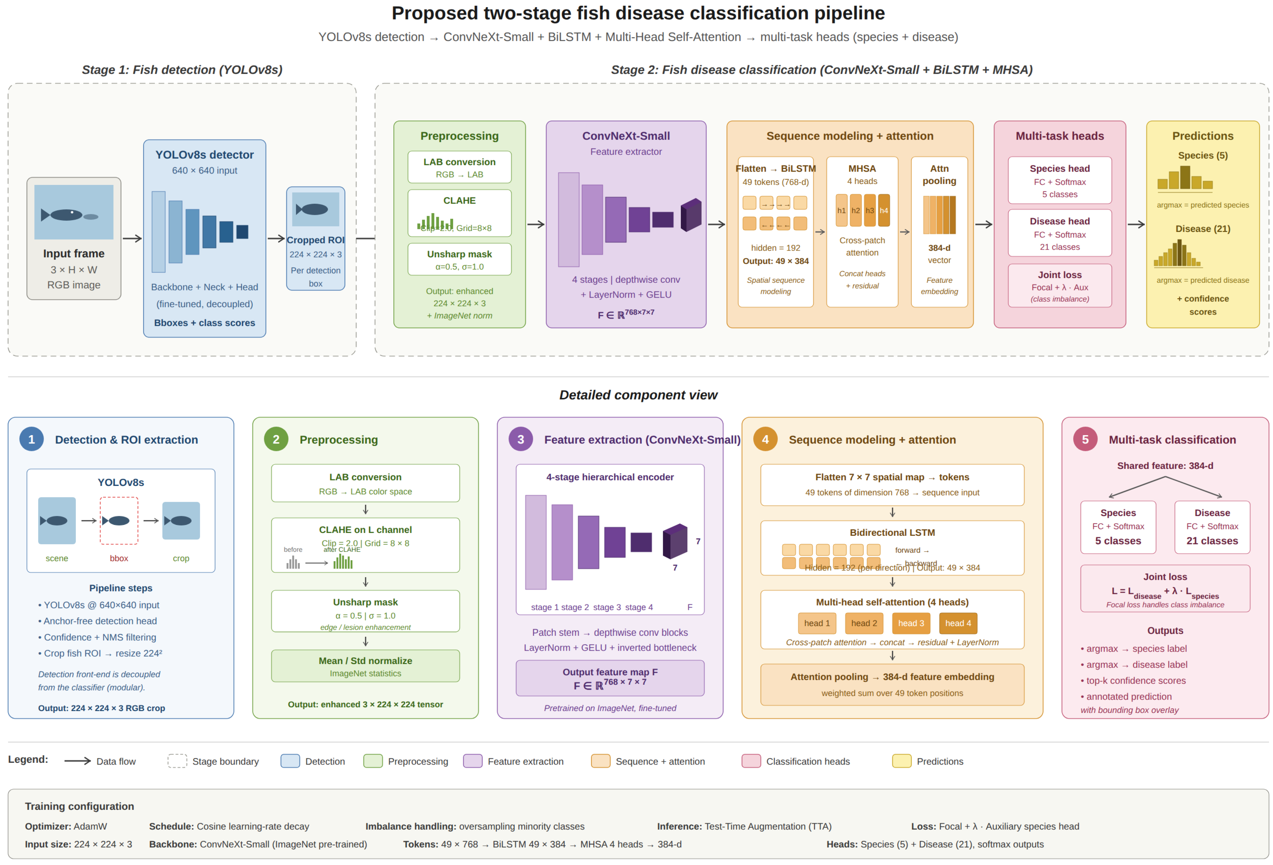
An overview of the proposed hybrid ConvNeXt–BiLSTM–MHSA framework is illustrated in Figure 1, which follows a two-stage design comprising fish instance detection and fine-grained disease–species classification. In the first stage, a YOLOv8s-based detector is employed to localize individual fish instances in raw underwater frames. In the second stage, the detected regions of interest are passed to a deep classification network that performs simultaneous fish species identification and disease recognition. The classification stage consists of a sequential processing pipeline including image preprocessing, hierarchical feature extraction using a ConvNeXt backbone, spatial–temporal dependency modeling via a BiLSTM encoder, and global context refinement using an MHSA module. The resulting representations are then used for multi-task prediction through parallel classification heads. The overall framework is further supported by a comprehensive learning strategy that includes class imbalance mitigation, loss optimization, progressive two-stage training, and test-time augmentation to enhance the robustness under challenging underwater imaging conditions such as low visibility, color distortion, and fine-grained inter-class similarity.

3.1. Proposed Architecture and System Pipeline

The proposed framework follows a two-stage decoupled design that separates fish localization from fine-grained pathological classification, addressing the competing optimization objectives that typically affect monolithic detection architectures. In the first stage, a YOLOv8s detector processes raw input frames $X\in {\mathbb{R}}^{3\times H\times W}$ captured from underwater cameras and generates a set of bounding box predictions $\mathcal{B}=\{b_1,b_2,\dots ,b_N\}$ localizing each fish instance within the scene. Each detected bounding box $b_i$ is cropped and resized to a standardized resolution of $224\times 224$ pixels, producing a region of interest $x_i$ suitable for downstream fine-grained analysis. In the second stage, each cropped fish image $x_i$ is forwarded to the ConvNeXt–BiLSTM–MHSA classifier, which produces simultaneous predictions for both the species identity ${\widehat{y}}_s\in {\mathbb{R}}^5$ and the disease state ${\widehat{y}}_d\in {\mathbb{R}}^{21}$. The classifier itself is composed of six tightly integrated sub-modules: (i) a Contrast-Limited Adaptive Histogram Equalization (CLAHE)-based preprocessing block that enhances the image contrast under variable underwater illumination; (ii) a ConvNeXt-Small convolutional backbone that extracts 768-dimensional feature descriptors over a $7\times 7$ spatial grid; (iii) a two-layer bidirectional LSTM encoder that models sequential dependencies across the flattened spatial tokens; (iv) a four-head self-attention block that performs non-sequential cross-patch reasoning; (v) an attention-weighted pooling head that aggregates the token sequence into a single discriminative embedding; and (vi) dual classification heads for disease and species prediction with multi-task learning. This decoupled design enables each architectural component to specialize fully in its designated task, while the shared backbone representation and auxiliary species supervision provide implicit regularization that improves generalization on the minority disease classes.

3.2. CLAHE-Based Image Preprocessing

Aquaculture underwater imagery is affected by significant visual degradation, such as wavelength-dependent light absorption, light scatter from suspended particles, and non-uniform illumination from artificial light sources, which reduces the visibility of subtle pathological patterns. To mitigate these effects and improve the consistency of input data distribution, we apply CLAHE as the first preprocessing step. Unlike global histogram equalization, which operates on the entire image and may amplify noise in homogeneous regions, CLAHE performs local contrast enhancement over small spatial regions while constraining amplification through a predefined clip limit. This enables the effective enhancement of fine structural details while suppressing noise amplification.

Specifically, each input crop x is first converted from RGB to the LAB color space, where the L (luminance) channel is decoupled from chromatic information $(a,b)$. CLAHE is applied exclusively to the L channel with a clip limit of $2.0$ and a tile grid size of $8\times 8$, producing an enhanced luminance channel $L^{\prime }$ while preserving the original chromatic signals. The enhanced LAB image is then converted back to RGB, yielding $x_{\mathrm{CLAHE}}$. To further enhance fine-grained structural information, an unsharp masking operation is applied as follows:

$$\tilde{x}=x_{\mathrm{CLAHE}}+\alpha \left(x_{\mathrm{CLAHE}}-{\mathcal{G}}_{\sigma }\left(x_{\mathrm{CLAHE}}\right)\right),$$

(1)

where ${\mathcal{G}}_{\sigma }$ denotes a Gaussian blur with standard deviation $\sigma =1.0$, and $\alpha =0.5$ controls the sharpening intensity. The subtraction term $x_{\mathrm{CLAHE}}-{\mathcal{G}}_{\sigma }\left(x_{\mathrm{CLAHE}}\right)$ yields a high-pass filtered representation that emphasizes local edge structures such as lesion boundaries, hemorrhagic regions, and fin deformities, which is then added back to the original enhanced image to produce a sharpened output $\tilde{x}$. This two-step preprocessing pipeline reduces the blue–green color bias that is prevalent in marine images and boosts the nuances of textural cues that are needed for detailed pathological differentiation at the same time.

3.3. ConvNeXt-Small Feature Extraction Backbone

The feature extraction backbone $f_{\theta }$ serves as the primary representation learning module of the proposed classification system, responsible for encoding the preprocessed input into a hierarchical feature map suitable for subsequent processing in a sequential manner. We adopt ConvNeXt-Small, a recent CNN architecture that outperforms Vision Transformers, while retaining the efficiency and biases of convolutional networks. ConvNeXt-Small is selected over alternative lightweight architectures such as EfficientNet-B2 and MobileNetV3 based on preliminary experiments, as it demonstrates superior capabilities in capturing subtle textural variations. This property is particularly important for distinguishing fine-grained disease patterns that exhibit minimal shape and color differences relative to healthy tissues.

The backbone transforms the preprocessed image $\tilde{x}\in {\mathbb{R}}^{3\times 224\times 224}$ in four stages, progressively reducing the spatial resolution while increasing the channel dimensionality. This results in a final feature tensor $F\in {\mathbb{R}}^{768\times 7\times 7}$, where each of the 49 spatial locations encodes a 768-dimensional feature vector combining local texture and high-level semantic information. The effectiveness of ConvNeXt-Small is attributed to several architectural design choices: (i) $7\times 7$ depthwise convolutions that expand the effective receptive field while maintaining computational efficiency; (ii) inverted bottleneck structures inspired by MobileNetV2 that enhance the representational capacity; and (iii) LayerNorm, which replaces BatchNorm to enhance the network stability, especially with small batch sizes, which are used in our gradient accumulation-based training approach. The backbone is initialized using ImageNet-22K pretrained weights to enable effective transfer learning from large-scale natural image distributions, which is particularly beneficial given the limited size of the fish disease dataset.

To facilitate sequential modeling in later stages, the 2D spatial feature map is flattened into a token sequence in row-major order, $Z\in {\mathbb{R}}^{49\times 768}$, where each token $z_t$ corresponds to a spatial location in the original $7\times 7$ feature grid. This transformation enables the subsequent BiLSTM and MHSA modules to model spatial relationships as a structured sequence of feature embeddings.

3.4. BiLSTM Spatial–Sequence Encoder

A key architectural selection that sets the proposed framework apart from purely convolutional and Transformer-based approaches is the integration of a BiLSTM layer applied to the flattened spatial token sequence. The motivation for incorporating BiLSTM is twofold. First, the BiLSTM imposes an explicit positional inductive bias over the spatial grid, providing stable gradient flow during early training epochs, when the self-attention mechanism is still learning to identify relevant token relationships. Second, the bidirectional formulation captures dependencies in both spatial directions simultaneously, modeling symptom correlations that may propagate along the fish body in either orientation.

Formally, the BiLSTM processes the input sequence $Z=[z_1,z_2,\dots ,z_{49}]$ in two parallel directions:

$$\begin{array}{cc}\hfill {\overrightarrow{h}}_t& ={\mathrm{LSTM}}_{\mathrm{fwd}}\left(z_t,{\overrightarrow{h}}_{t-1},{\overrightarrow{c}}_{t-1}\right),\hfill \end{array}$$

(2)

$$\begin{array}{cc}\hfill {\overleftarrow{h}}_t& ={\mathrm{LSTM}}_{\mathrm{bwd}}\left(z_t,{\overleftarrow{h}}_{t+1},{\overleftarrow{c}}_{t+1}\right),\hfill \end{array}$$

(3)

$$\begin{array}{cc}\hfill h_t& =\left[{\overrightarrow{h}}_t\parallel {\overleftarrow{h}}_t\right]\in {\mathbb{R}}^{384},\hfill \end{array}$$

(4)

where ${\overrightarrow{h}}_t$ and ${\overleftarrow{h}}_t$, respectively, denote the forward and backward hidden states at position t, and the symbol ‖ represents concatenation along the feature dimension. The internal LSTM cell operations follow the standard gated formulation with input, forget, and output gates, and we employ two stacked layers to provide sufficient representational depth for capturing hierarchical spatial patterns. The hidden dimension is set to 192 per direction, yielding a total output dimension of 384 after concatenation. Applied across all 49 spatial tokens, this produces the encoded sequence $H=[h_1,h_2,\dots ,h_{49}]\in {\mathbb{R}}^{49\times 384}$.

The BiLSTM effectively establishes a spatial reading order over the feature grid, encoding relationships such as the co-occurrence of hemorrhagic spots in one body region with ulceration in another. Such dependencies are typically overlooked by global pooling operations and only weakly modeled by purely convolutional hierarchies. This reading-order paradigm has proven highly effective in recent CNN–BiLSTM hybrid architectures for medical imaging classification and agricultural disease recognition, and we extend this principle to the domain of fish disease recognition for the first time.

3.5. Multi-Head Self-Attention Block

While the BiLSTM captures sequential positional dependencies, it processes tokens according to a fixed row-major traversal order and cannot directly model arbitrary long-range relationships between spatially distant tokens. To overcome this limitation and enable flexible cross-patch reasoning, we introduce a four-head self-attention module that operates on the BiLSTM output sequence H. The multi-head attention mechanism allows the model to attend to different representational subspaces in parallel, capturing diverse relationship patterns such as species-specific body proportions, cross-regional symptom correlations, and structural symmetries.

For each attention head $i\in \{1,2,3,4\}$, the input sequence H is linearly projected into query, key, and value representations:

$$Q_i=H{W}_i^Q,K_i=H{W}_i^K,V_i=H{W}_i^V,$$

(5)

where $W_i^Q,W_i^K,W_i^V\in {\mathbb{R}}^{384\times 96}$ are learnable projection matrices producing a per-head dimension of $d_k=96$. Scaled dot-product attention is then computed as

$${\mathrm{head}}_i=\mathrm{Attn}(Q_i,K_i,V_i)=\mathrm{softmax}\left({\displaystyle \frac{Q_i{K}_i^{\top }}{\sqrt{d_k}}}\right)V_i,$$

(6)

where the scaling factor $\sqrt{d_k}$ prevents the softmax from saturating when the dot products grow large in magnitude. The outputs of all four heads are concatenated and linearly projected back to the original dimensionality:

$$A=\mathrm{Concat}({\mathrm{head}}_1,{\mathrm{head}}_2,{\mathrm{head}}_3,{\mathrm{head}}_4)W^O,$$

(7)

where $W^O\in {\mathbb{R}}^{384\times 384}$ is the output projection matrix. To stabilize training and facilitate gradient flow, a complete Transformer-style block is formed by surrounding the attention operation with residual connections and layer normalization, followed by a position-wise feed-forward network (FFN):

$$\begin{array}{c}{H}^{\prime }=\mathrm{LayerNorm}(H+A),\end{array}$$

(8)

$$\begin{array}{c}M=\mathrm{LayerNorm}(H^{\prime }+\mathrm{FFN}\left(H^{\prime }\right)),\end{array}$$

(9)

where the FFN consists of two linear transformations with GELU activation in between, expanding the intermediate dimension to $4\times 384=1536$ before projecting back to 384. The final output of this block is $M\in {\mathbb{R}}^{49\times 384}$, representing contextually enriched token representations that encode both local sequential dependencies and global cross-patch relationships.

3.6. Attention-Weighted Pooling

To aggregate the sequence of contextualized tokens M into a single discriminative embedding suitable for classification, we employ an attention-weighted pooling mechanism that learns to prioritize diagnostically relevant spatial locations. This approach generalizes global average pooling by assigning location-specific importance weights learned end-to-end with the classification objective, following the self-attentive pooling paradigm.

For each token position t, an attention score $a_t$ is computed through a small two-layer network with tanh nonlinearity:

$$a_t=w^{\top }tanh(W_a{m}_t+b_a),$$

(10)

where $W_a\in {\mathbb{R}}^{128\times 384}$ and $w\in {\mathbb{R}}^{128}$ are learnable parameters, and $b_a$ is a bias vector. The scalar scores across all 49 positions are then normalized via softmax to produce a valid probability distribution,

$${\alpha }_t={\displaystyle \frac{exp\left(a_t\right)}{{\sum }_{j=1}^{49}exp\left(a_j\right)}},$$

(11)

and the final pooled embedding is computed as a weighted sum of the token representations:

$$e={\displaystyle \sum _{t=1}^{49}}{\alpha }_t{m}_t\in {\mathbb{R}}^{384}.$$

(12)

This learned pooling strategy allows the model to automatically discover the most informative spatial regions for disease classification, effectively implementing a soft attention-based region-of-interest selection mechanism that typically concentrates on body regions such as the eyes, fins, and lateral line, where pathological symptoms most commonly manifest.

3.7. Dual Classification Heads with Multi-Task Learning

The pooled embedding e is simultaneously fed into two parallel classification heads that share the same underlying representation but produce distinct predictions, implementing a hard parameter sharing multi-task learning paradigm.

The primary disease classification head predicts the 21-class disease–species joint label through a two-layer MLP with GELU activation:

$${\widehat{y}}_d=W_{d2}·\mathrm{GELU}(W_{d1}e+b_{d1})+b_{d2},$$

(13)

where $W_{d1}\in {\mathbb{R}}^{256\times 384}$ and $W_{d2}\in {\mathbb{R}}^{21\times 256}$, producing logits over 21 classes, corresponding to the Cartesian product of five health statuses across four primary species plus the additional Neobchi category.

The auxiliary species classification head predicts the five-class species identity through a similar two-layer MLP:

$${\widehat{y}}_s=W_{s2}·\mathrm{GELU}(W_{s1}e+b_{s1})+b_{s2},$$

(14)

where $W_{s1}\in {\mathbb{R}}^{128\times 384}$ and $W_{s2}\in {\mathbb{R}}^{5\times 128}$. This auxiliary supervision forces the backbone to learn species-discriminative features that would otherwise be suppressed when training solely on the 21-class disease objective, where species information appears only as a conditioning factor within each compound label. The species head incurs no additional inference cost at deployment time, as it can be optionally disabled once training is complete, yet its presence during training provides implicit regularization that demonstrably improves the minority disease recall.

4. Training Strategy and Optimization

4.1. Loss Formulation

To address the severe class imbalance inherent in the fish-project dataset, where healthy species classes contain over 1100 samples while minority disease classes contain as few as 31 samples, we employ the focal loss with frequency-based class weighting. The focal loss downweights well-classified examples to focus training on hard, often misclassified minority class instances.

For a probability prediction ${\widehat{p}}_c$ for class c with ground-truth indicator $y_c$, the focal loss is formulated as

$${\mathcal{L}}_{\mathrm{focal}}(y,\widehat{p})=-\sum _{c\in \mathcal{C}}{\alpha }_c{y}_c{(1-{\widehat{p}}_c)}^{\gamma }log{\widehat{p}}_c,$$

(15)

where $\gamma =2.0$ is the focusing parameter that controls the rate at which easy examples are downweighted, and ${\alpha }_c$ is a class-dependent weighting coefficient. Following the class balance principle while avoiding the extreme weighting that can destabilize training, we define

$${\alpha }_c={\displaystyle \frac{1}{\sqrt{n_c}}}·{\displaystyle \frac{1}{Z}},$$

(16)

where $n_c$ is the training sample count for class c, and Z is a normalization constant ensuring ${\sum }_c{\alpha }_c=\left|\mathcal{C}\right|$. The √-inverse-frequency formulation produces weights in the moderate range of $[0.23,1.39]$ for our dataset, avoiding the catastrophic overweighting (range $[0.25,8.3]$) observed in preliminary experiments with pure inverse-frequency weighting, which caused the majority class recall to collapse to zero.

The total multi-task objective combines the disease classification loss with a weighted auxiliary species classification term:

$${\mathcal{L}}_{\mathrm{total}}={\mathcal{L}}_{\mathrm{focal}}^{\left(d\right)}+\lambda {\mathcal{L}}_{\mathrm{focal}}^{\left(s\right)},$$

(17)

where $\lambda =0.3$ controls the relative contribution of the species auxiliary task. This value was selected through a systematic grid search over $\lambda \in \{0.1,0.2,0.3,0.5,1.0\}$, with $\lambda =0.3$ providing the optimal balance between the primary disease objective and the regularization benefit of species supervision.

4.2. Class Imbalance Mitigation Strategy

To tackle the serious long-tailed distribution problem, we use a combined approach that includes targeted oversampling, weighted sampling, and regularization-based data augmentation. This strategy mitigates two common failure modes typically observed with naive imbalance handling: (i) majority class collapse (where aggressive minority weighting causes the model to entirely ignore majority classes) and (ii) overfitting on duplicated minority samples (where excessive oversampling leads to memorization rather than generalization).

• Targeted oversampling.

Based on an empirical analysis of the per-class validation performance in preliminary experiments, eight visually subtle defect categories—primarily eye and fin defects, characterized by a limited spatial extent and high inter-class similarity—are identified as the most challenging and are oversampled by $15\times$, replicating each image 15 times in the effective training set. The remaining disease classes (bleeding and ulcer variants) are oversampled by $5\times$. Healthy species classes retain their original frequency without oversampling. Based on the class distribution detailed in Section 5.1, we construct an oversampled training set, as summarized in

Table 2. Per-class sample counts before and after targeted oversampling.

Class	Original	Oversampled	Factor
Healthy species classes (5).	5595	5595	$1\times$
chamdom-eyedefect	34	510	$15\times$
chamdom-findefect	41	615	$15\times$
doldom-eyedefect	85	1275	$15\times$
doldom-findefect	37	555	$15\times$
gamseongdom-eyedefect	38	570	$15\times$
gamseongdom-findefect	42	630	$15\times$
jopi-eyedefect	36	540	$15\times$
jopi-findefect	38	570	$15\times$
Other disease classes (8)	296	1480	$5\times$
Total	6242	12,340	—

. The per-class sample counts before and after oversampling show that the effective training set size increases from 6242 to 12,340 images, significantly enhancing the contribution of minority classes without distorting the overall distribution.

• Weighted random sampling.

Complementing static oversampling, we employ a WeightedRandomSampler during mini-batch construction. Each training sample i is assigned a sampling weight that is inversely proportional to the square root of its class frequency in the oversampled dataset:

$$w_i\propto {\displaystyle \frac{1}{\sqrt{n_{c\left(i\right)}}}},$$

(18)

where $c\left(i\right)$ denotes the class of sample i, and $n_{c\left(i\right)}$ is the number of samples in that class after oversampling. This formulation ensures approximately balanced mini-batches, with the consistent representation of both majority and minority classes throughout training.

• Mixup and CutMix augmentation.

To further improve generalization and prevent memorization of the replicated minority samples, we apply Mixup and CutMix augmentations with probability $p=0.2$ each. Mixup creates convex combinations of training pairs with mixing coefficient ${\lambda }_m\sim \mathrm{Beta}(0.2,0.2)$, while CutMix replaces a random rectangular patch of one image with content from another. These augmentations provide smoothness regularization in both the input and label spaces, mitigating overfitting on the oversampled minority classes.

4.3. Two-Stage Progressive Training Strategy

The training procedure follows a two-stage progressive schedule designed to balance the rapid convergence of newly initialized components with the stable adaptation of the pretrained backbone. This strategy, derived from the empirical analysis of training dynamics, consistently outperformed single-stage fine-tuning in our ablation studies.

• Stage 1:

In the first stage, all parameters of the ConvNeXt-Small backbone are frozen (requires_grad$=$False), and only the newly introduced components—the BiLSTM encoder, MHSA block, attention-weighted pooling, and dual classification heads—are trained. This isolation allows the randomly initialized modules to reach a reasonable operating point without disrupting the pretrained backbone representations. Training uses the OneCycleLR schedule with a maximum learning rate of $3\times {10}^{-3}$, with a linear warm-up for the first 30% of iterations followed by cosine annealing for the remainder. This aggressive learning rate is appropriate because only the head parameters (approximately 2.8 M) are being updated, and these components benefit from the rapid initial exploration of the loss landscape.

• Stage 2:

In the second stage, the backbone is unfrozen and the entire network is trained end-to-end, but with carefully differentiated learning rates reflecting the different sensitivities of pretrained versus newly trained components. The backbone uses a low learning rate of $5\times {10}^{-5}$ to gently adapt the ImageNet-22K pretrained features to the fish disease domain, while the heads use a higher learning rate of $5\times {10}^{-4}$ to continue refining their task-specific representations. Both learning rates follow a smooth cosine annealing schedule without warm restarts, which was empirically found to produce more stable convergence than the warm-restart variant. Early stopping with patience of 12 epochs is applied based on the validation macro F1-score.

• Optimization details.

Optimization throughout both stages uses AdamW with weight decay $0.05$, ${\beta }_1=0.9$, ${\beta }_2=0.999$, and $ϵ={10}^{-8}$. To manage GPU memory constraints, we employ gradient checkpointing (trading compute for memory by recomputing intermediate activations during the backward pass), mixed-precision training in FP16, and gradient accumulation over 2 micro-batches of 32 images each, yielding an effective batch size of 64. Gradient clipping with a maximum $L_2$ norm of $1.0$ is applied to prevent occasional gradient explosions during mixed-precision training.

Table 3. Hyperparameter configuration for the two-stage progressive training schedule.

Parameter	Stage 1	Stage 2
Epochs	15	60
Backbone status	Frozen	Unfrozen (full fine-tune)
LR schedule	OneCycleLR	Cosine annealing
Max LR (backbone)	—	$5\times {10}^{-5}$
Max LR (heads)	$3\times {10}^{-3}$	$5\times {10}^{-4}$
Warm-up ratio	30%	—
Optimizer	AdamW	AdamW
Weight decay	0.05	0.05
$\beta 1$, $\beta 2$	0.9, 0.999	0.9, 0.999
Effective batch size	64	64
Mixed precision	FP16	FP16
Gradient clipping	1.0	1.0
Early stopping patience	—	12
Mixup probability	0.2	0.2
CutMix probability	0.2	0.2
Focal $\gamma$	2.0	2.0
Species weight $\lambda$	0.3	0.3

presents the complete specification of the training configuration to ensure the full reproducibility of the reported results. The most important selections in the hyperparameters, including the $10\times$ learning rate difference between the backbone and heads in Stage 2, and the transition from OneCycleLR to cosine annealing across stages, were validated through controlled experiments. These components are therefore integral to the training protocol rather than arbitrary hyperparameter selections.

4.4. Test-Time Augmentation

To further improve the prediction robustness and calibration, particularly on minority classes, we apply five-view test-time augmentation (TTA) during inference. For each test image, five augmented variants are constructed: the original preprocessed image, a horizontally flipped version, and three center-cropped versions at scale factors $0.9$, $1.0$, and $1.1$. Each variant is forwarded through the network independently, and the resulting softmax probabilities are averaged as

$${\widehat{p}}_{\mathrm{TTA}}\left(y\right|x)={\displaystyle \frac{1}{K}}{\displaystyle \sum _{k=1}^K}\mathrm{softmax}\left(f\left({\mathcal{T}}_k\left(x\right)\right)\right),$$

(19)

where ${\mathcal{T}}_k$ denotes the k-th augmentation transform, $f(·)$ is the trained network, and $K=5$. The final prediction is the argmax of the averaged distribution. TTA provides two key benefits: it reduces prediction variance by averaging over multiple related views, and it mitigates the impact of minor localization errors in the upstream detector by providing multiple aligned crops of the same fish.

5. Experimental Setup

5.1. Dataset

The experimental evaluation is conducted on the publicly available fish-project dataset, distributed via Roboflow under the CC BY 4.0 license [2]. The dataset consists of underwater images of four Korean marine aquaculture species—Chamdom (striped beakfish, Oplegnathus fasciatus), Doldom (black sea bream, Acanthopagrus schlegelii), Gamseongdom (Korean rockfish, Sebastes schlegelii), and Jopi-bollag (red sea bream, Pagrus major)—along with an additional category labeled Neobchi. Each species is annotated with five health conditions: healthy, bleeding, ulcer, eye defect, and fin defect. After excluding underrepresented categories with insufficient samples, the final classification task comprises 21 classes.

The dataset follows the standard split provided by the original source, containing 6242 training images, 260 validation images, and 282 test images. As summarized in

Table 4. Dataset distribution across species, conditions, and splits.

Species	Condition	Train	Validation	Test
Chamdom	Healthy	1148	12	32
	Bleeding	35	6	8
	Ulcers	38	4	4
	Eye Defect	34	6	8
	Fin Defect	41	4	4
Doldom	Healthy	1058	92	46
	Bleeding	42	3	4
	Ulcers	31	4	8
	Eye Defect	85	7	8
	Fin Defect	37	2	9
Gamseongdom	Healthy	1147	21	30
	Bleeding	39	4	7
	Ulcers	36	5	7
	Eye Defect	38	5	6
	Fin Defect	42	2	6
Jopi-bollag	Healthy	1136	16	47
	Bleeding	38	6	1
	Ulcers	37	3	5
	Eye Defect	36	6	8
	Fin Defect	38	3	5
Neobchi	Healthy	1106	49	29
Total		6242	260	282

, the dataset exhibits a pronounced class imbalance, where healthy classes contain over 1000 samples each, while disease-related classes are significantly underrepresented, often with fewer than 100 samples per class. The long-tailed distribution observed in the dataset, where healthy specimens significantly outnumber diseased instances, is consistent with patterns reported in operational aquaculture monitoring studies, where the disease prevalence typically ranges from 5% to 15% of the population [16]. However, we acknowledge that this distribution was shaped by the dataset curation process, and the exact ratios may vary across different farming systems, species, and seasonal conditions.

5.2. Evaluation Metrics

To comprehensively evaluate the proposed framework and ensure a fair comparison with existing methods, we employ a set of standard metrics encompassing both classification and detection performance.

Accuracy. The overall classification accuracy measures the fraction of test samples for which the predicted class matches the ground truth:

$$\mathrm{Accuracy}={\displaystyle \frac{1}{N}}{\displaystyle \sum _{i=1}^N}⊮[{\widehat{y}}_i=y_i],$$

(20)

where $⊮[·]$ is the indicator function, N is the total number of test samples, and ${\widehat{y}}_i$ and $y_i$ denote the predicted and ground-truth labels, respectively.

Top-k accuracy. For fine-grained classification, top-k accuracy measures the fraction of samples for which the true label appears among the model’s top-k predictions:

$$\mathrm{Top}-k\mathrm{Acc}={\displaystyle \frac{1}{N}}{\displaystyle \sum _{i=1}^N}⊮[y_i\in {\mathrm{top}}_k\left({\widehat{p}}_i\right)].$$

(21)

Per-class precision, recall, and F1-score. For each class c, let ${\mathrm{TP}}_c$, ${\mathrm{FP}}_c$, and ${\mathrm{FN}}_c$ denote the true positives, false positives, and false negatives, respectively. The per-class precision, recall, and F1-score are defined as

$$\begin{array}{cc}\hfill {\mathrm{Precision}}_c& ={\displaystyle \frac{{\mathrm{TP}}_c}{{\mathrm{TP}}_c+{\mathrm{FP}}_c}},\hfill \end{array}$$

(22)

$$\begin{array}{cc}\hfill {\mathrm{Recall}}_c& ={\displaystyle \frac{{\mathrm{TP}}_c}{{\mathrm{TP}}_c+{\mathrm{FN}}_c}},\hfill \end{array}$$

(23)

$$\begin{array}{cc}\hfill \mathrm{F}{1}_c& ={\displaystyle \frac{2·{\mathrm{Precision}}_c·{\mathrm{Recall}}_c}{{\mathrm{Precision}}_c+{\mathrm{Recall}}_c}}.\hfill \end{array}$$

(24)

Precision measures the proportion of correct predictions among all predictions assigned to class c, recall measures the proportion of true class-c instances that were correctly identified, and F1 is their harmonic mean.

Macro-averaged metrics. To provide a single aggregated score that treats all classes equally regardless of their frequency—a particularly important consideration for imbalanced datasets—we compute the macro-averaged precision, recall, and F1 by averaging the per-class values:

$$\mathrm{Macro}-\mathrm{F}1={\displaystyle \frac{1}{\left|\mathcal{C}\right|}}\sum _{c\in \mathcal{C}}\mathrm{F}{1}_c.$$

(25)

The macro F1 is the primary ranking metric for our evaluation because it prevents majority class dominance from masking poor minority class performance.

Weighted-averaged metrics. Weighted averages compute per-class metrics weighted by class frequency, providing a more globally representative score:

$$\mathrm{Weighted}-\mathrm{F}1=\sum _{c\in \mathcal{C}}{\displaystyle \frac{n_c}{N}}\mathrm{F}{1}_c,$$

(26)

where $n_c$ is the number of test samples in class c.

Macro AUC (Area Under the ROC Curve). For each class c, the binary one-vs-rest receiver operating characteristic (ROC) curve is constructed by varying the decision threshold on the predicted probability ${\widehat{p}}_c$. The AUC for class c is

$${\mathrm{AUC}}_c={\int }_0^1{\mathrm{TPR}}_c\left({\mathrm{FPR}}_c\right)d\left({\mathrm{FPR}}_c\right),$$

(27)

where ${\mathrm{TPR}}_c$ and ${\mathrm{FPR}}_c$ denote the true positive rate and false positive rate, respectively. The macro AUC is the unweighted average of the per-class AUCs:

$$\mathrm{Macro}-\mathrm{AUC}={\displaystyle \frac{1}{\left|\mathcal{C}\right|}}\sum _{c\in \mathcal{C}}{\mathrm{AUC}}_c.$$

(28)

Mean Average Precision (mAP). For direct comparison with detection baselines including RT-GalaDet, we compute the mean average precision at an intersection over union (IoU) threshold of $0.5$, denoted ${\mathrm{mAP}}_{50}$. The average precision for class c is the area under the precision–recall curve:

$${\mathrm{AP}}_c^{@0.5}={\int }_0^1{\mathrm{Precision}}_c\left(r\right)dr,$$

(29)

where the integral is evaluated at all recall levels $r\in [0,1]$ using the all-point interpolation strategy adopted by the COCO evaluation protocol. The ${\mathrm{mAP}}_{50}$ averages the $\mathrm{AP}$ values across all classes:

$${\mathrm{mAP}}_{50}={\displaystyle \frac{1}{\left|\mathcal{C}\right|}}\sum _{c\in \mathcal{C}}{\mathrm{AP}}_c^{@0.5}.$$

(30)

Frames Per Second (FPS). Inference throughput is measured as the number of images processed per second during single-batch inference on a standard GPU:

$$\mathrm{FPS}={\displaystyle \frac{N_{\mathrm{images}}}{T_{\mathrm{total}}}},$$

(31)

where $T_{\mathrm{total}}$ is the total wall-clock inference time. FPS measurements are performed with batch size 1 to emulate real-time deployment conditions. This metric is critical in assessing the feasibility of deploying the model in practical multi-camera aquaculture monitoring systems.

5.3. Implementation Environment

Table 5. Experimental setup and training configuration.

Category	Details
Framework	PyTorch 2.2 (CUDA 12.1)
Hardware	NVIDIA RTX 4090 (24 GB VRAM)
Input Resolution (Classifier)	$224\times 224$
Input Resolution (Detector)	$640\times 640$
Detector Model	YOLOv8s (Ultralytics 8.1.0)
Optimizer (Detector)	SGD ($lr=0.01$, momentum $0.937$)
Weight Decay	$5\times {10}^{-4}$
LR Schedule	Cosine annealing
Training Epochs (Detector)	100
Random Seed	42 (NumPy, PyTorch, CUDA deterministic)
Libraries	torchvision 0.17, OpenCV 4.8, scikit-learn 1.3
Python Version	Python 3.10
Training Time	∼3.5 h (Classifier), ∼1.2 h (Detector)

summarizes the hardware, the software environment, and the key training configurations used in this study. The setup ensures reproducibility through fixed random seeds and deterministic computation, while leveraging high-performance GPU acceleration for efficient model training.

6. Results

In this section, we present a comprehensive experimental evaluation of the proposed ConvNeXt–BiLSTM–MHSA hybrid framework, including analyses of the detection and classification performance, end-to-end pipeline comparisons, systematic ablation studies, and a qualitative assessment of model behavior.

6.1. Dataset Distribution Analysis

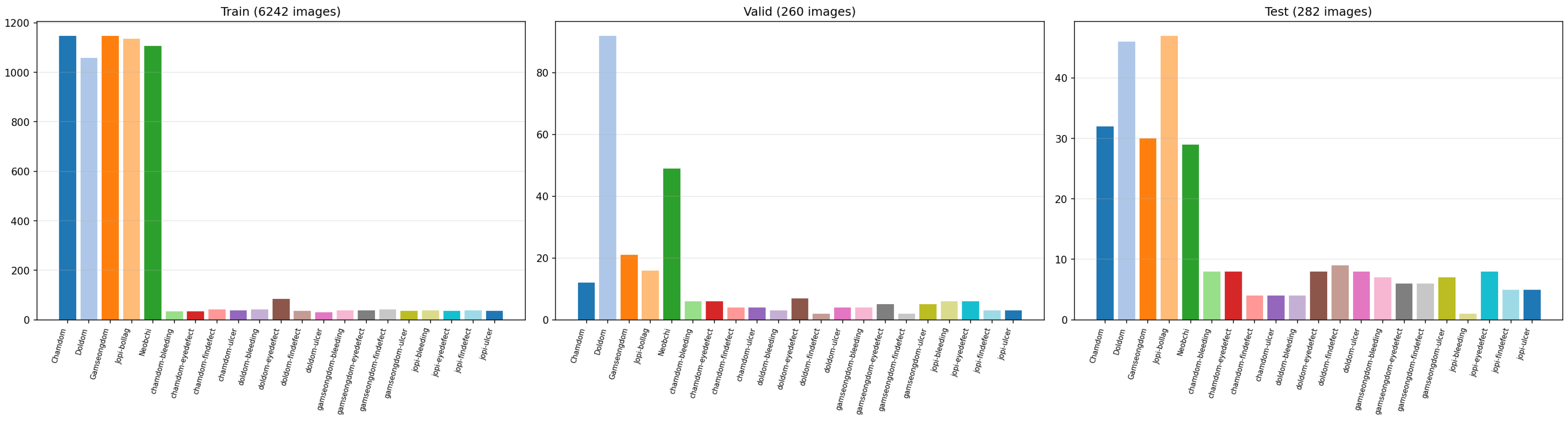
Figure 2 provides a detailed illustration of the class frequency distribution across all three dataset splits. The training distribution (left panel) exhibits an extreme long-tailed pattern characteristic of real-world aquaculture monitoring data, where healthy specimens naturally outnumber diseased ones by several orders of magnitude. The five healthy species classes (Chamdom, Doldom, Gamseongdom, Jopi-bollag, and Neobchi) collectively account for 5595 of the 6242 training samples (89.6%), while the 16 disease-specific classes together comprise only 647 samples (10.4%). The doldom-eyedefect class stands as an outlier among disease classes, with 85 training samples, while several other minority classes contain as few as 31–42 samples.

The validation and test distributions (middle and right panels) exhibit a similar but less extreme pattern, with the Doldom healthy class being particularly prominent in validation (93 samples) due to the standard curator-provided split. This distributional similarity between train and test ensures that the model is evaluated on data drawn from the same underlying population, while the class imbalance in both splits reflects the operational reality that any deployed system must be capable of correctly identifying rare disease cases amid predominantly healthy populations.

6.2. Training Dynamics Analysis

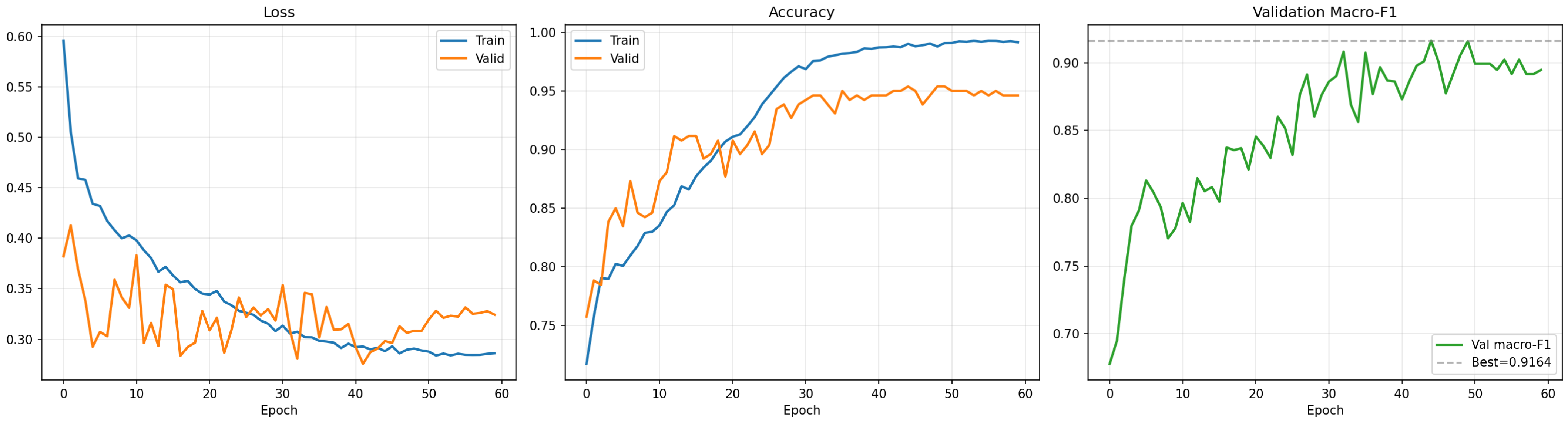
Figure 3 illustrates the training dynamics during Stage 2 fine-tuning. Three key observations from these curves validate the effectiveness of the proposed training strategy.

(1) 

Stable optimization under class imbalance.

The loss curves (left panel) show stable convergence without divergence, despite the aggressive oversampling of minority classes. This confirms that the square-root inverse-frequency focal loss weighting is well calibrated and avoids the majority class collapse observed with more extreme weighting schemes. The training loss decreases monotonically from $0.60$ at epoch 1 to approximately $0.285$ at epoch 60, while the validation loss exhibits higher variance due to the limited validation set size but follows a consistent downward trend, stabilizing near $0.28$.

(2) 

Effect of data augmentation on accuracy dynamics.

The accuracy curves (center panel) reveal an initial phase (first ∼15 epochs) where the validation accuracy exceeds the training accuracy. This behavior arises from the use of Mixup and CutMix, which generate interpolated training samples and thereby distort the training accuracy estimate, while validation is performed on clean samples. After approximately epoch 20, the training and validation curves intersect, and the typical situation (training > validation) is restored. The final gap between the training accuracy (∼99%) and validation accuracy (∼95%) remains small, indicating effective generalization with minimal overfitting.

(3) 

Importance of macro F1 for imbalanced learning.

The macro F1 curve (right panel) highlights the necessity of optimizing a class-balanced metric. While the validation accuracy saturates at around epoch 30, the macro F1 continues to improve until approximately epoch 45, reaching a peak value of $0.9164$. This indicates continued gains on minority classes, which have a limited impact on the accuracy but significantly influence the macro F1. Accordingly, model selection is based on the validation macro F1 to ensure balanced performance across all 21 classes, rather than biasing toward majority classes.

6.3. Classification Results

Table 6. Classification metrics on the 282-image test set.

Metric	Value
Top-1 Accuracy	94.33%
Top-3 Accuracy	98.94%
Top-5 Accuracy	100.00%
Macro Precision	97.11%
Macro Recall	90.88%
Macro F1-Score	0.9264
Weighted F1-Score	0.9370
Macro AUC	0.994
Classes at 100% Recall	14/21

summarizes the classification performance of the proposed framework on the 282-image test set using five-view test-time augmentation. The model achieves top-1 accuracy of 94.33%, which increases to 98.94% and 100.00% for the top-3 and top-5 accuracy, respectively. This indicates that misclassifications are typically confined to closely related classes, with the correct label consistently appearing among the top-ranked predictions. The macro-averaged F1-score of 0.9264 demonstrates strong and balanced per-class performance. Similarly, the macro AUC of 0.994 indicates near-perfect separability across different decision thresholds. A key observation is that, for 14 out of 21 classes, the model achieves 100% recall, meaning that no test samples from these classes are missed. The remaining classification errors are concentrated primarily in four visually subtle eye defect categories and three partially confused majority species classes. These error patterns are further analyzed in the confusion matrix.

The test set of 282 images, while standard for curated aquaculture datasets, presents statistical limitations for a 21-class fine-grained classification problem. Several minority disease categories contain fewer than 10 test samples, making the per-class recall and AUC estimates for these categories susceptible to higher variance and sensitivity to individual predictions; therefore, such metrics should be interpreted as indicative rather than definitive measures of model capability.

The results in Table 6 further reveal a notable imbalance between the macro precision (97.11%) and macro recall (90.88%) of $6.2$ percentage points. This indicates that the model is highly reliable when assigning positive predictions (high precision) but occasionally fails to detect certain minority class instances (lower recall), particularly in visually subtle categories. From an application perspective, this trade-off is preferable for aquaculture health monitoring. False positives (low precision) would lead to unnecessary interventions and increased operational costs, whereas false negatives (low recall) can be mitigated through continuous monitoring across multiple frames, increasing the likelihood of eventual detection.

6.4. Confusion Matrix Analysis

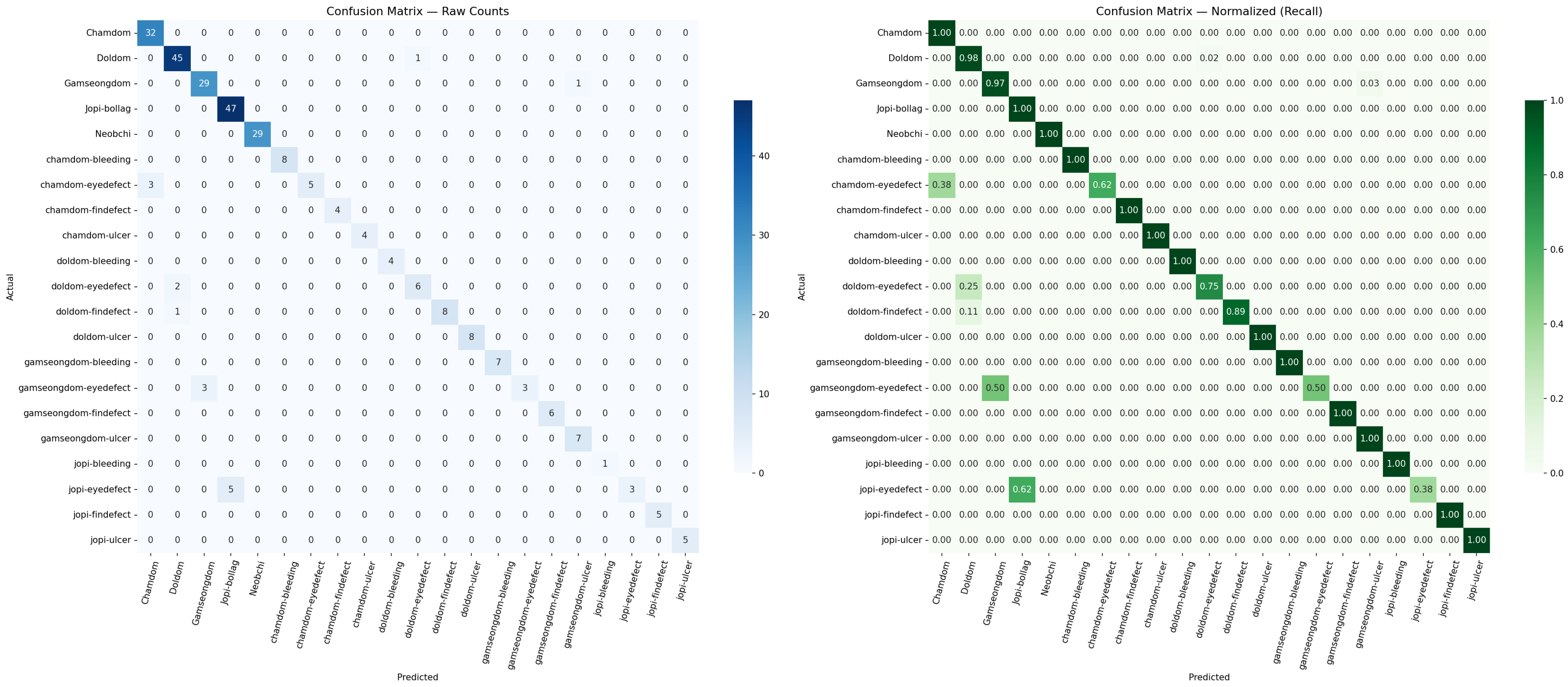
Figure 4 presents both raw-count and row-normalized confusion matrices, providing detailed insights into the classification behavior of the proposed framework. The dominant diagonal structure in both representations confirms the strong overall performance, while the off-diagonal entries reveal three consistent and diagnostically meaningful error patterns.

• Pattern 1: Eye defect to healthy species confusion.

The most prominent errors arise from the misclassification of eye defect samples as their corresponding healthy species classes. For example, chamdom-eyedefect yields 62% recall (3/8 misclassified as Chamdom (healthy)), doldom-eyedefect yields 75% recall (2/8 misclassified as Doldom (healthy)), and doldom-findefect yields 89% recall (1/9 misclassified as Doldom (healthy)). These errors stem from the inherently subtle nature of eye-related defects, which are often spatially small, exhibit weak visual contrast, and may be partially occluded or poorly captured under challenging imaging conditions. In such ambiguous cases, the model exhibits a bias toward the dominant healthy class, consistent with the underlying class distribution.

• Pattern 2: Minor cross-species confusion.

Limited confusion is observed within majority healthy species classes—that is, one Doldom (healthy) sample is predicted as Doldom-bleeding (yielding 98% recall) and one Gamseongdom (healthy) sample as Gamseongdom-ulcer (97% recall). From an application perspective, such errors are relatively benign in clinical terms, as they would trigger additional inspection rather than resulting in missed detections.

• Pattern 3: Cross-species eye defect ambiguity.

The most challenging cases involve eye defect categories, where inter-class similarity leads to reduced recall. For instance, Gamseongdom-eyedefect yields 50% recall (3/6 misclassified as healthy), and Jopi-eyedefect yields 38% recall (5/8 misclassified as healthy). Notably, Jopi-eyedefect yields 100% precision but low recall, indicating a conservative prediction strategy in which the model favors the dominant healthy species label when confidence in disease-specific features is low. This behavior is influenced by the auxiliary species classification head, which provides strong species-level cues that can override the weaker disease signal when the pathological features are ambiguous.

Despite these localized error patterns, the confusion matrix remains highly diagonal with minimal cross-class confusion. All bleeding classes, three of four ulcer classes, and most fin defect classes exhibit near-perfect classification, demonstrating the robustness of the proposed framework under severe class imbalance and limited training data.

6.5. Per-Class Performance Analysis

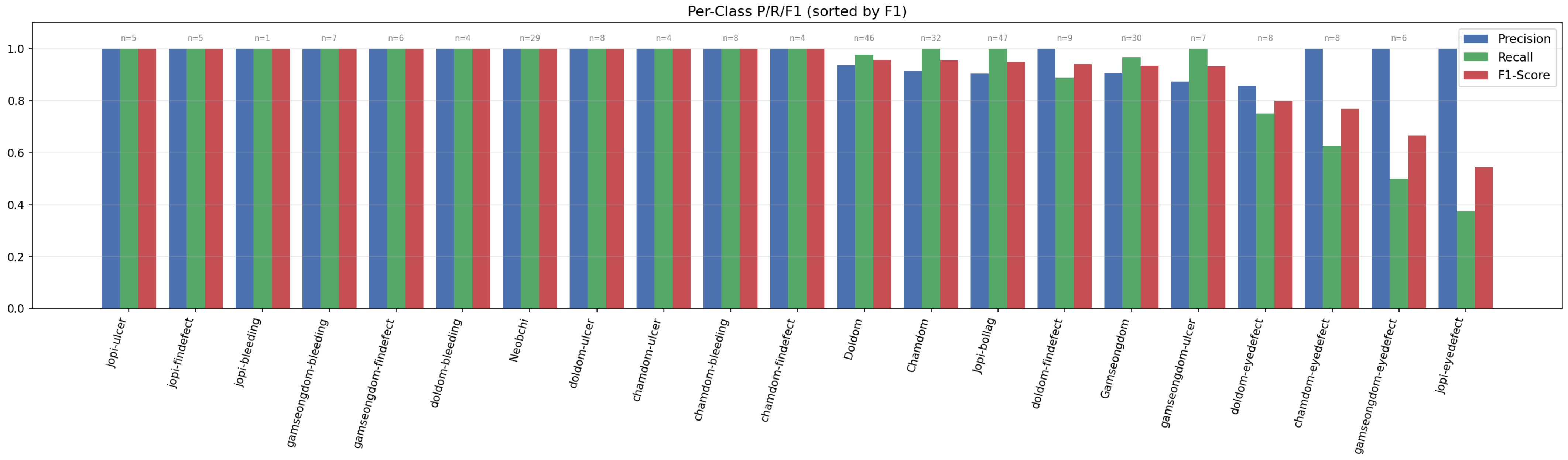
Figure 5 presents a per-class breakdown of the precision, recall, and F1-score, providing fine-grained insights into model behavior that complement the aggregate metrics reported in Table 6. The classes are sorted by F1-score in descending order, revealing clear, three-tier performance stratification.

• Tier 1 (F1 = 1.0):

Eleven classes achieve perfect precision, recall, and F1-scores, including multiple bleeding, ulcer, and fin defect categories. Notably, several of these classes contain only four to eight test samples, yet all instances are correctly classified, indicating strong generalization despite limited data.

• Tier 2 (F1 = 0.93–0.96):

Six classes fall within the upper-moderate performance range, including the majority of healthy species classes (e.g., Doldom, Chamdom, Jopi-bollag, Gamseongdom) and a few disease categories. Minor reductions in the F1-score are primarily due to occasional intra-species confusion, as previously discussed, but the overall performance remains robust.

• Tier 3 (F1 = 0.54–0.80):

Four eye defect classes form a distinct lower-performance group, with F1-scores ranging from 0.54 to 0.80. These classes exhibit consistently high precision (86–100%) but reduced recall (37.5–75%), indicating a conservative prediction bias. The jopi-eyedefect class is the most challenging (F1 = 0.54, recall = 37.5%), reflecting the combined effects of subtle visual cues, inter-class similarity, and limited training samples.

This stratified analysis highlights that the proposed framework achieves reliable performance across most classes, while identifying eye defect categories as the primary source of residual error. From a deployment perspective, the predictions for Tier 1 and Tier 2 classes can be considered highly reliable, whereas Tier 3 classes may benefit from additional verification due to their lower recall.

6.6. ROC Curve Analysis

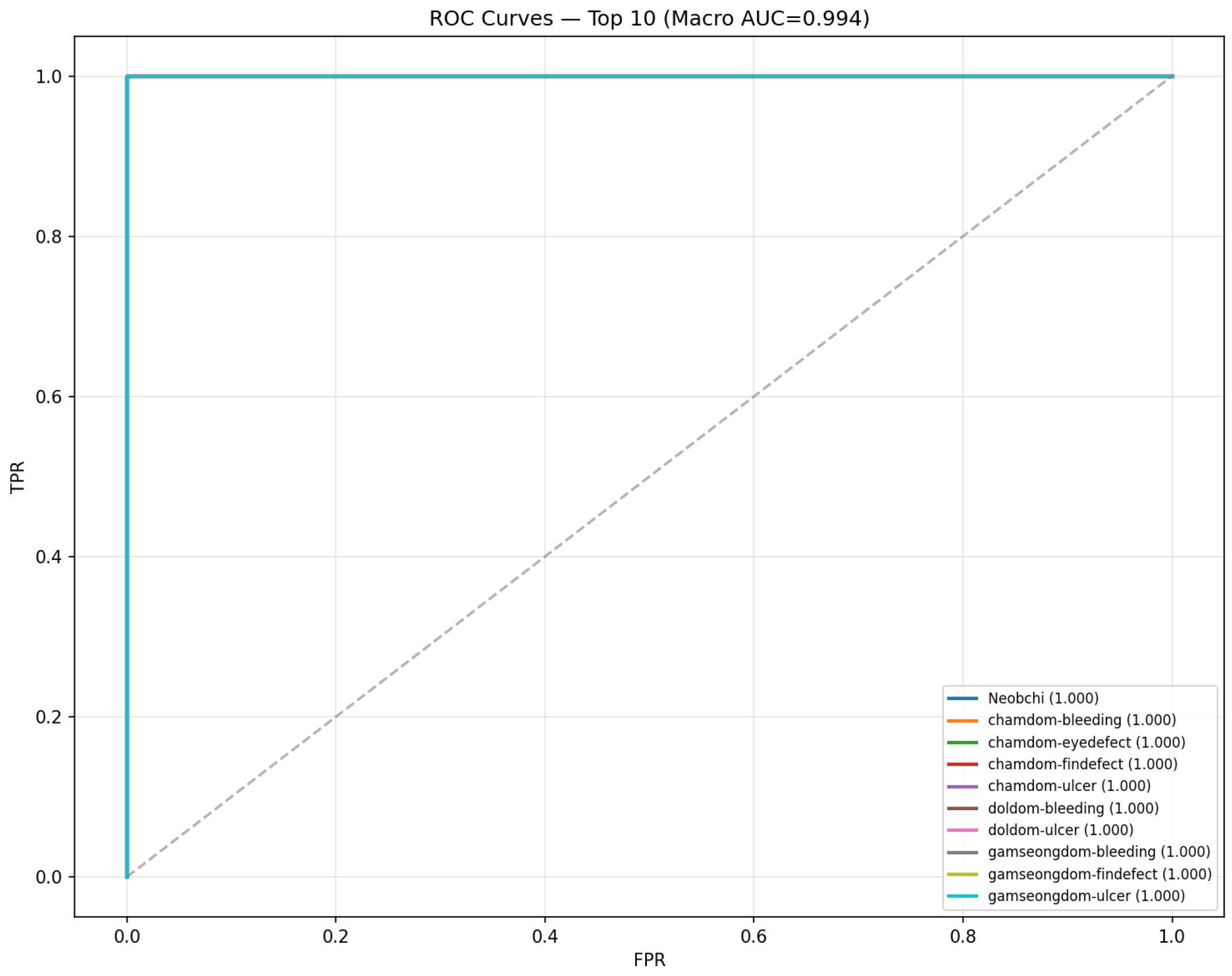
Figure 6 presents the one-vs-rest ROC curves for the ten highest-performing classes (ranked by AUC), along with the macro-averaged AUC of 0.994 across all 21 classes. The curves closely follow the upper-left boundary, with ten classes achieving an AUC of 1.000, indicating near-perfect separability between positive and negative samples.

For these classes, there exists an operating threshold at which the true positive rate approaches 1 while the false positive rate approaches 0, corresponding to ideal classification performance. This behavior confirms that the learned feature representations are highly discriminative for the majority of classes.

The reported macro AUC of 0.994 reflects strong overall performance, even when accounting for more challenging categories such as eye defect classes, whose AUC values range between 0.85 and 0.95. Importantly, these values still indicate good ranking capabilities, suggesting that most misclassifications arise from threshold-dependent decision boundaries rather than insufficient feature representation.

This observation has practical implications: by adjusting the class-specific decision thresholds, particularly for minority and visually subtle categories such as eye defects, it is possible to trade a small reduction in precision for a meaningful gain in recall. Such flexibility is valuable in aquaculture monitoring systems, where missing diseased instances may be more critical than generating additional false alarms.

The proposed framework is intended as an assistive early screening tool for detecting visually observable fish disease symptoms and continuous health monitoring, rather than as a replacement for comprehensive veterinary diagnosis, which additionally requires laboratory analysis, microbiological testing, environmental assessment, and expert clinical interpretation. It acts as a triage system, identifying potentially affected individuals who are flagged for prioritized examination by veterinary experts.

6.7. Qualitative Prediction Analysis

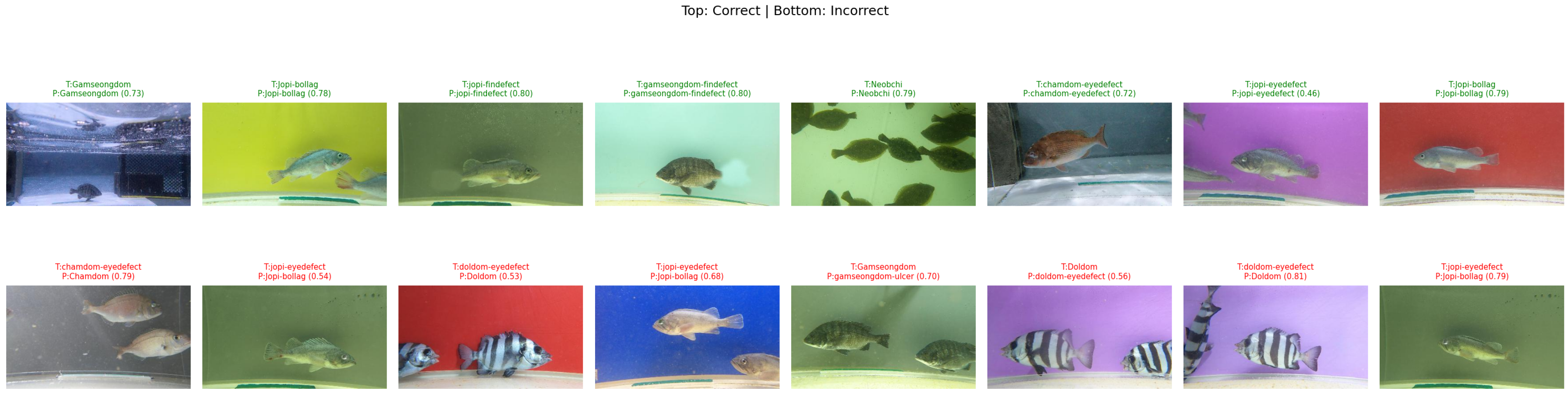
Figure 7 provides a qualitative assessment of the model through representative test samples. The top row shows correctly classified examples under significant visual variability, including diverse water colors, fish poses, and disease manifestations. Notably, a chamdom eye-defect case (confidence 0.72) is correctly identified despite subtle visual cues, indicating the model’s ability to detect fine-grained pathological features when sufficiently visible.

The bottom row presents representative misclassifications, all belonging to eye defect categories. These errors generally yield lower confidence scores (0.46–0.81) compared to correct predictions (0.72–0.80), suggesting that uncertainty-aware thresholding could be leveraged during deployment. Specifically, low-confidence predictions can be flagged for human review, enabling a semi-automated workflow that balances efficiency with reliability.

Examining the specific error modes, we observe confusions such as T:chamdom-eyedefect → P:Chamdom, T:jopi-eyedefect → P:Jopi-bollag, and T:doldom-eyedefect → P:Doldom. These results align with the confusion matrix analysis, confirming that the primary challenge lies in detecting subtle eye region abnormalities, while species-level discrimination remains robust due to the auxiliary classification head.

6.8. End-to-End Pipeline Demonstration

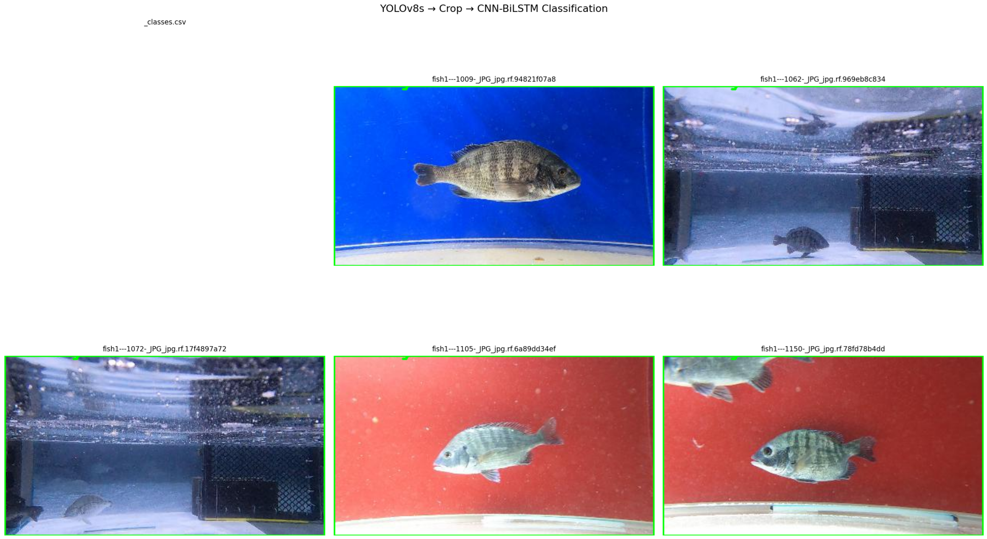
Figure 8 illustrates the complete two-stage inference pipeline on representative test images. The YOLOv8s detector localizes fish instances under challenging conditions, including small-scale targets, partial occlusions, boundary regions, and multi-fish scenes. The resulting bounding boxes are used to extract object-centric crops that serve as inputs to the classification module.

This decoupled design separates localization and fine-grained recognition into two specialized models, enabling independent optimization for each task. The detector is optimized for high-recall fish localization across complex underwater backgrounds, while the classifier operates on cropped regions with an improved signal-to-noise ratio, facilitating the more accurate discrimination of visually similar disease patterns.

From a system perspective, this modular formulation enhances the flexibility and maintainability, as either stage can be updated or replaced (e.g., newer YOLO variants or alternative classifiers) without retraining the entire pipeline, making the framework suitable for iterative deployment in aquaculture monitoring systems.

6.9. End-to-End Detection Pipeline Comparison

Table 7. Comparison with existing detection approaches on the fish-project dataset.

Model	Precision	Recall	mAP50	mAP50-95	FPS
YOLOv8s [44]	86.4%	85.7%	89.8%	79.8%	—
YOLO11s [44]	86.4%	84.1%	85.3%	75.1%	—
YOLO12s [45]	93.8%	80.1%	84.7%	75.4%	—
YOLOX [46]	78.6%	83.6%	90.6%	80.1%	—
RTDETR-Resnet18 [2]	94.6%	87.9%	88.7%	78.5%	—
RTDETR-L [35]	96.1%	87.7%	87.8%	78.1%	—
NanoDet-m [35]	61.7%	64.9%	74.2%	61.7%	—
RT-GalaDet [2]	93.3%	89.7%	89.0%	79.0%	51.98
Ours (YOLOv8s + ConvNeXt–BiLSTM–MHSA)	97.1%	90.9%	96.1%	—	213.3
Ours vs. RT-GalaDet	+3.8	+1.2	+7.1	—	+161.3 (4.1×)

compares the proposed YOLOv8s + ConvNeXt–BiLSTM–MHSA pipeline with existing state-of-the-art models. The proposed framework achieves the best overall performance in terms of precision, recall, mAP, and inference speed, indicating a clear Pareto improvement over existing methods.

The precision improves from 93.3% (RT-GalaDet) to 97.1%. This gain is primarily attributed to the decoupled detection–classification design, where YOLOv8s provides accurate region proposals and the classifier focuses exclusively on fine-grained disease discrimination using tightly cropped regions. This separation improves the discrimination ability of the classifier for visually subtle minority classes. Recall increases from 89.7% to 90.9%, confirming that the improvement is not achieved at the expense of sensitivity. The gain is consistent with the proposed oversampling strategy, which enhances the representation of challenging eye defect and fin defect categories and improves the detection of rare pathological patterns. The most significant improvement is observed in the mAP₅₀, which increases from 89.0% to 96.1%. This indicates stronger overall ranking quality across confidence thresholds and reflects improved joint precision–recall behavior rather than simple threshold tuning. The proposed pipeline achieves 213.3 FPS, corresponding to a 4.1× speed-up over RT-GalaDet (51.98 FPS). This improvement is mainly due to (i) classification on cropped $224\times 224$ regions instead of full-resolution frames and (ii) the inherent computational efficiency of the ConvNeXt-Small backbone at inference time. The resulting throughput is sufficient for real-time multi-camera aquaculture deployment.

FPS assessment is performed in a single GPU (batch size 1) to simulate real-time deployment. The reported 213.3 FPS is for the fully end-to-end pipeline (YOLOv8s detection on $640\times 640$ frames and ConvNeXt–BiLSTM–MHSA classification on $224\times 224$ cropped regions) with single-view inference and no test-time augmentation. The accurate throughput drops to about 42.7 FPS with the five-view TTA function, which is acceptable in many aquaculture monitoring applications, where accuracy is desired over peak performance.

Overall, the results demonstrate that the proposed pipeline improves both the detection accuracy and computational efficiency, achieving consistent gains over recent YOLO- and RT-DETR-based baselines.

6.10. Ablation Study

To systematically evaluate the contribution of each architectural component and training strategy, we perform an ablation study in which key components are removed from the full model while keeping all other settings unchanged. The results in

Table 8. Ablation experiments showing the impact of removing each key component from the proposed framework.

Configuration	Accuracy (%)	Macro F1
Full model (Ours)	94.33	0.9264
— w/o MHSA block	91.93 (−2.40)	0.8964 (−0.030)
— w/o BiLSTM encoder	92.43 (−1.90)	0.9024 (−0.024)
— w/o CLAHE preprocessing	93.13 (−1.20)	0.9144 (−0.012)
— w/o auxiliary species head	93.53 (−0.80)	0.9184 (−0.008)
— w/o focal loss (CE only)	92.51 (−1.82)	0.8954 (−0.031)

confirm that each component contributes non-redundantly to the overall performance, with distinct functional roles.

The MHSA module contributes the most significant performance gain, as substituting MHSA with average pooling over the output of BiLSTM leads to the largest degradation in both accuracy (−2.40%) and the macro F1-score (−0.030). This indicates that non-sequential cross-patch reasoning is essential for distinguishing subtle pathological features that manifest as correlations between spatially distant body regions. Without MHSA, the model relies solely on the sequential processing of the BiLSTM, which cannot effectively link features from opposite ends of the fish body.

The BiLSTM encoder provides the second most important contribution. Replacing the BiLSTM with a layer with the same number of parameters caused a drop in performance (−1.90% accuracy, −0.024 macro F1), demonstrating that the sequential feature modeling introduces a beneficial spatial inductive bias for capturing structured local dependencies. This complements MHSA by stabilizing optimization and enhancing local context modeling.

Replacing the focal loss with standard cross-entropy leads to the most pronounced degradation in the macro F1 (−0.031), highlighting its effectiveness in addressing class imbalances. The focusing mechanism is critical for learning from hard minority class samples and cannot be fully compensated for by class reweighting alone.

Removing CLAHE preprocessing reduces the accuracy by 1.20%, indicating that contrast enhancement improves the visibility of fine-grained lesion patterns under degraded underwater imaging conditions, thereby facilitating more discriminative feature extraction.

The removal of the auxiliary species head leads to measurable performance degradation under focal loss (−0.80% accuracy, −0.008 macro F1), indicating the benefit of multi-task regularization. This effect is primarily reflected in the detailed per-class analysis, which shows reduced recall for minority and species-specific disease classes, suggesting that the auxiliary branch encourages the backbone to learn more discriminative species-aware representations that improve class separation in visually similar categories.

Overall, the ablation results demonstrate that the performance gains arise from the synergistic integration of all components rather than any single module, validating the design of the proposed framework for long-tailed fine-grained classification in aquaculture environments.

The proposed CNN–BiLSTM–MHSA framework achieves state-of-the-art performance for fish disease detection, improving both the accuracy and efficiency over existing baselines while operating at 213.3 FPS. Overall, the proposed framework demonstrates that decoupling localization and fine-grained recognition, combined with hybrid spatial–sequence modeling and targeted imbalance handling, holds strong potential for detecting visually observable abnormalities in aquaculture environments. The observed improvements across accuracy, robustness, and inference speed confirm its suitability for real-time deployment in practical monitoring systems. These gains reflect synergistic rather than merely additive interactions among components; the MHSA module benefits from BiLSTM-stabilized token sequences, while species head regularization achieves the maximum effectiveness in conjunction with focal loss weighting. This interdependent behavior supports the unified architectural design, wherein the components function as an integrated whole rather than independent optional modules.

6.11. Limitations

Despite the strong performance of the proposed framework, the results of this study should be interpreted in light of several limitations:

• Eye defect recall remains 37.5–75%; this is a dataset artifact, since eye defects are physically small and visually subtle, and the problem is aggravated by limited samples. Mamba-style longer-range backbones may help.
• Our pipeline assumes a reliable front-end crop; very occluded fish are dropped by YOLOv8s.
• The dataset presents notable limitations, including absent metadata on housing and annotation conditions, restricted coverage to five Korean marine species with unverified cross-species generalizability, and potential distributional biases stemming from its multi-source, non-standardized assembly.

7. Conclusions

This study addresses the problem of simultaneous fish species identification and fine-grained disease classification in marine aquaculture by proposing a CNN–BiLSTM–MHSA hybrid framework that reformulates surface disease screening as a spatial–sequence classification task with auxiliary species supervision. Unlike detection-centric approaches that jointly learn localization and classification within a single network, the proposed method decouples these tasks into a YOLOv8s detection front-end and a ConvNeXt-Small–BiLSTM–MHSA classifier, enabling task-specific optimization at each stage. The framework further incorporates CLAHE-based preprocessing, focal loss with square-root inverse-frequency class weighting, targeted $15\times$ oversampling of minority classes, an auxiliary species head for multi-task regularization, and a two-stage progressive training strategy with differential learning rates under mixed precision. Experiments on the fish-project benchmark (four species, five health conditions, 21 fine-grained classes) demonstrate state-of-the-art performance across all metrics. The classification module achieves 94.33% top-1 accuracy, a 0.9264 macro F1-score, and a 0.994 macro AUC, with 14/21 classes reaching 100% recall. The end-to-end pipeline attains 97.1% precision, 90.9% recall, 96.1% mAP₅₀, and 213.3 FPS, outperforming recent baselines in both accuracy and speed. Ablation studies confirm that all components contribute non-redundantly, with MHSA providing the largest single gain. The achieved throughput exceeds the practical requirements for multi-camera aquaculture monitoring, supporting real-time deployment. Overall, the results validate the decoupled detection–classification paradigm with spatial–sequence hybrid modeling as an effective and efficient solution for fine-grained aquaculture health screening.