


Abstract
Dolphins are widely recognized as intelligent marine mammals with sophisticated communication and echolocation. Accurately classifying their whistles is essential for understanding their communication patterns and monitoring their population size, structure, and distribution. In this study, we assembled a large, high-quality dataset of Indo-Pacific bottlenose dolphin (Tursiops aduncus) whistle signals collected at the Chimelong Ocean Kingdom. The dataset included multiple whistle categories, including a whistle type that has not previously been available for research. We then applied convolutional neural networks (CNNs) for classifying whistle signals, using five CNN architectures to analyze the signals. Model performance was evaluated using mean average precision (mAP), and the best-performing model achieved 0.929 in mAP on the test set, demonstrating that CNN-based approaches can effectively distinguish among different whistle classes. To probe robustness, we also introduced noise at defined SNR levels to increase testing complexity and assess the stability of the classifier. BELLHOP acoustic propagation modeling was used to generate channel impulse responses. These simulated signals were combined with the original signal data to construct an augmented training set. The results indicate that this augmentation enhanced the robustness of the classification model. Differentiating the whistle types is crucial as whistle categories may reflect variation in communication structure, behavioral context, or group-level acoustic patterns. Therefore, the proposed approach can support large-scale bioacoustic analysis and provide useful information for future studies on dolphin communication, behavior, and conservation.
1. Introduction
Dolphins have an exceptional sonar system to adapt to their living environment, and their acoustic signals are commonly grouped into three major categories, which are echolocation clicks, whistles, and the burst-pulse signal [1,2]. The echolocation clicks are short-duration, broadband pulse signals used for underwater navigation, localization, foraging, and obstacle avoidance [1,2]. The whistle signals are tonal, frequency-modulated signals that play a crucial role in social communication, including group cohesion, individual recognition, and long-distance contact [3,4]. The last one is burst-pulse signals that consist of rapidly repeated pulsed signals and have been associated with several behavioral contexts, including social interactions, agonistic behavior, feeding, and close-range communication [5].
Among all these acoustic signals, whistles work especially well for contour-based classification. Their frequency patterns change over time, and we can easily describe and analyze these patterns using time–frequency representations. The fundamental frequencies of dolphin whistles are typically reported from approximately 0.5 to 24 kHz, and their durations usually range from 0.1 to 2 s, although longer whistles may occur in specific behavioral or social contexts [4]. Previous studies have classified dolphin whistles according to frequency modulation contours, such as ascending, descending, sinusoidal, U-shaped, concave, convex, constant, and multi-component patterns [6,7,8]. These contour-based categories provide a practical way to describe whistle structure and form the basis for many manual and automated classification studies.
Signature whistles further demonstrate the biological relevance of whistle contours. They are individually distinctive frequency-modulated calls that can encode caller identity and support social contact, group cohesion, and individual recognition [9,10]. Studies have shown that dolphins can recognize or generalize signature whistle contours, suggesting that contour shape may remain important even when other acoustic features vary [10]. Therefore, frequency modulation patterns are not only useful acoustic descriptors but may also be associated with individual identity and social behavior.
The Indo-Pacific bottlenose dolphin (Tursiops aduncus) is a medium-sized cetacean in the family Delphinidae. Compared with the common bottlenose dolphin (Tursiops truncatus), it is generally more slender and often shows speckling on the ventral surface. This species inhabits warm coastal and shelf waters across the Indian Ocean and western Pacific [11]. It is adaptable, feeds mainly on fish and cephalopods, and is frequently observed in coastal habitats where interactions with human activities may occur. In China, this species is listed as a nationally protected Class II animal. Therefore, studying its acoustic signals is important for passive acoustic monitoring, behavioral analysis, and conservation management.
Traditional studies of whistle classification have often relied on manually measured acoustic parameters, including start frequency, end frequency, minimum and maximum frequency, center frequency, duration, and the number of inflection points [12]. Other studies have used contour similarity or rule-based descriptions to distinguish whistle types [13]. Although these approaches provide interpretable features, they may not fully capture complex time–frequency structures in large-scale whistle datasets. Deep learning methods, especially convolutional neural networks (CNNs), provide an alternative approach by learning discriminative features directly from spectrograms or other time–frequency representations. CNN-based approaches have been widely and successfully used for audio tagging, sound event detection, and marine mammal acoustic classification [14,15,16]. Even so, applying these methods to dolphin whistle classification is still quite challenging. This is because existing datasets usually have a small volume, uneven recording quality, and inconsistent annotation standards.
Current publicly available datasets for marine mammal acoustics [17,18,19] are constrained by small sample sizes, low signal-to-noise ratios, unstable recording environments, and unclear label annotations. As a result, models trained on these datasets often achieve only limited accuracy in detection and recognition tasks. Furthermore, there is still a lack of standardized frameworks for training and evaluating reliable dolphin whistle classification models.
Another important challenge is that dolphin acoustic signals recorded in natural environments are affected by underwater propagation and ambient noise. Propagation effects may distort whistle signals through multipath arrival, transmission loss, and channel-dependent spectral variation. Underwater acoustic models, such as BELLHOP, can simulate high-frequency sound propagation and generate channel impulse responses under specified environmental conditions [20]. Such simulations provide a useful way to augment acoustic datasets and evaluate whether classification models remain robust under channel-affected conditions.
To tackle these problems, this work builds a high-quality whistle dataset for Tursiops aduncus. The acoustic recordings were collected in a relatively quiet, well-controlled environment and manually labeled by professional experts. We also establish a complete workflow to train and test deep CNN models for reliable dolphin whistle classification. In particular, we compare multiple classic CNN structures, taking the time–frequency features of whistle signals as model input. To make the model adapt better to complex underwater acoustic scenarios, we use the BELLHOP model to simulate underwater sound propagation of dolphin whistles, and enrich the dataset by adding real-world ocean background noise. These newly generated synthetic data are then used to boost model generalization and verify the stability of the classification models under realistic interference.
The key contributions of this work are summarized as follows: (1) We built a high-quality, fully labeled whistle dataset for Indo-Pacific bottlenose dolphins, which included a new whistle type that has not been included in existing research datasets before. (2) We conducted a systematic evaluation of multiple CNN models for contour-based dolphin whistle classification tasks. (3) We adopted BELLHOP-based underwater channel simulation and ocean noise data augmentation to enhance the overall robustness of classification models in complex underwater acoustic environments.
The remainder of the paper is organized as follows. Section 2 describes the collection, annotation, and pre-processing of Tursiops aduncus whistle signals from Chimelong Ocean Kingdom, and also presents the CNN architectures and simulation methods. Section 3 reports the classification and robustness evaluation results. Section 4 discusses the biological and methodological implications of the findings. Section 5 concludes the paper and outlines future work.
2. Methodology
2.1. Data Collection and Annotation
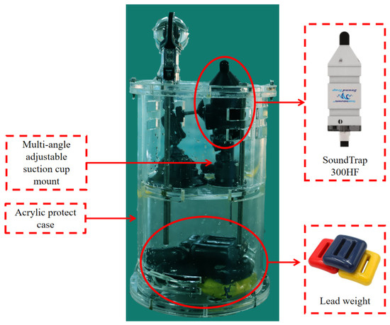
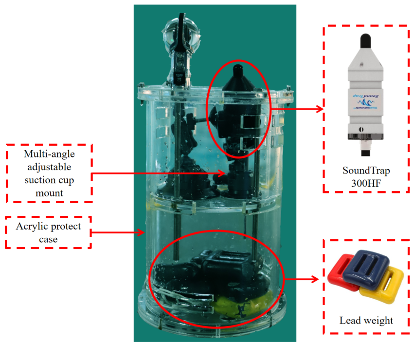
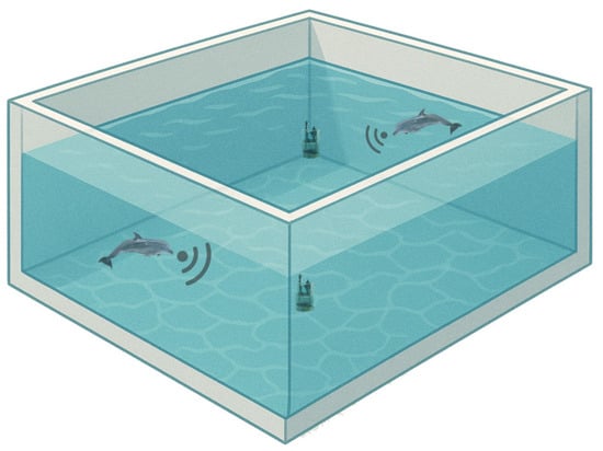
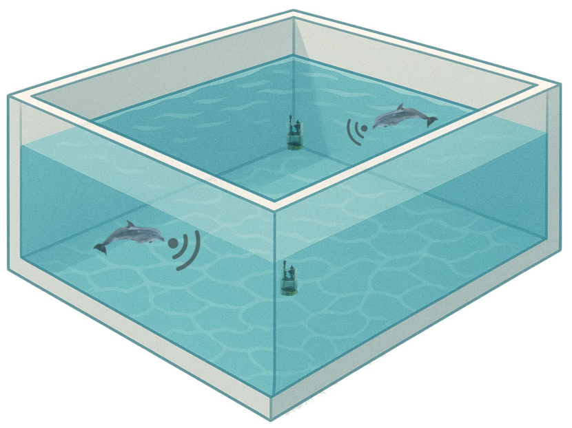
The raw data were collected at the dolphin aquarium of Chimelong Ocean Kingdom in Zhuhai, China. Two self-contained hydrophones (SoundTrap 300 HF, Ocean Instruments, Auckland, New Zealand) were used, each enclosed in a custom acrylic housing to prevent dolphins from accessing the devices. The hydrophones use a 16-bit SAR ADC. Therefore, each signal sample was recorded with 16-bit resolution. This hydrophone was selected because its 20 Hz–150 kHz bandwidth and high sampling capability are suitable for dolphin acoustic signal monitoring, and the 16-bit resolution provides sufficient amplitude precision for time–frequency analysis and CNN-based classification. As shown in Figure 1, the cylindrical housing has two sections: the upper section holds adjustable suction-cup mounts for the hydrophone and an underwater camera, and the lower section contains lead weights to ensure stability underwater. The hydrophones were deployed at two locations in the pool, as shown in Figure 2: one at the center to capture signals from all directions, and another in a corner, positioned safely out of the dolphins’ reach. The hydrophones recorded signals at a sampling frequency of 144 kHz from five Tursiops aduncus—two adults and three infants—in a single large pool.
Figure 1.
Hydrophone setup.
Figure 2.
Underwater hydrophone deployment.
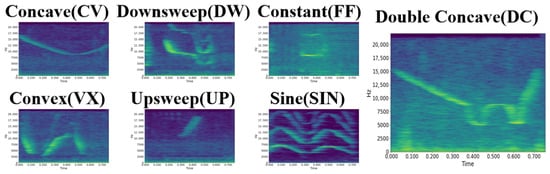
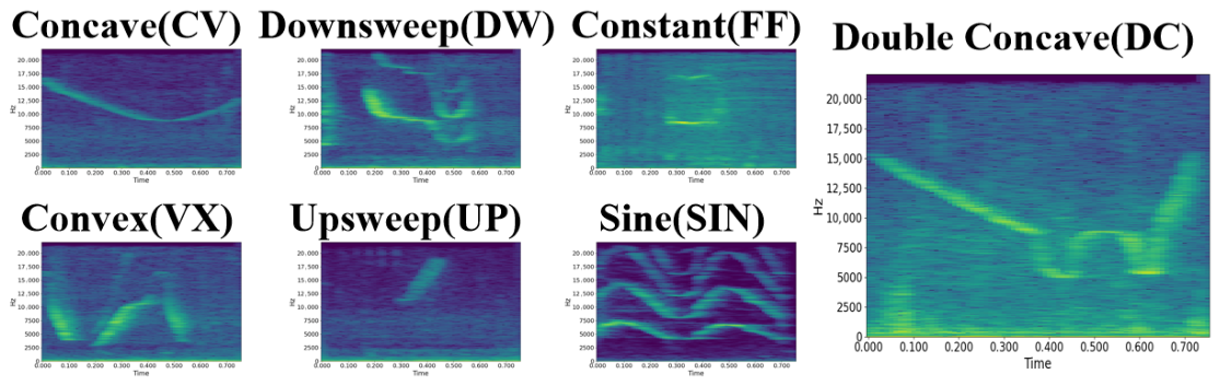
The raw dataset contains approximately 72 h of recordings. Since the signals were recorded in a large pool with low ambient noise, the whistle signals exhibit relatively high signal-to-noise ratios. In this study, we manually annotated 19.5 h of recordings following the category definitions of Xue Rui-chao et al. [8], with the addition of a new class termed double concave, as this structure is frequently observed during the annotation process. The seven whistle types are defined as: constant, nearly flat contour with frequency variation under 1 kHz across the time span of the signal; upsweep, the fundamental frequency increases over time; downsweep, the fundamental frequency decreases over time; concave, the fundamental frequency first decreases, then increases over time; convex, the fundamental frequency first increases, then decreases over time; sine, sinusoidal-like contour; double concave, two consecutive concave contours concatenated together.
All these seven whistle samples are visualized in Figure 3.
Figure 3.
Seven typical Tursiops aduncus whistle signals.
The annotated dataset includes the start and end times of each whistle in the raw recordings, along with its call type. In total, 3913 samples were labeled, and the dataset statistics are summarized in Table 1. The classes are imbalanced—for example, the convex type has 912 samples, whereas the constant type has only 256. Overall, the whistles span a frequency range of approximately 3–40 kHz.
Table 1.
Annotated dataset details.
2.2. Data Pre-Processing
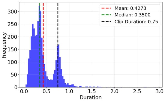
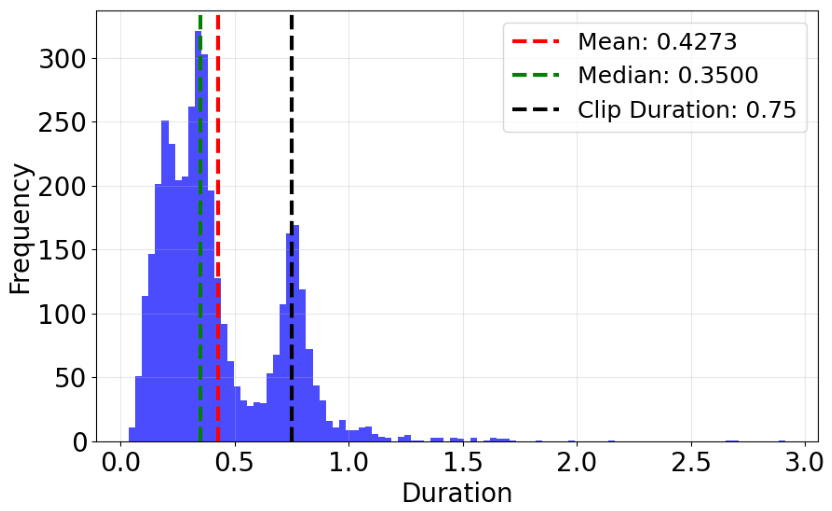
The whistle signals were cropped into 0.75 s segments. For signals longer than 0.75 s, the central 0.75 s segment of the original recording was used. For shorter signals, the segment was extended by including additional portions from the original recording at both ends to reach the target length. As shown in Figure 4, 0.75 s corresponds to roughly the 85th percentile, ensuring that most whistle contours are complete.
Figure 4.
The distribution of whistle signal lengths.
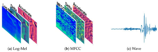
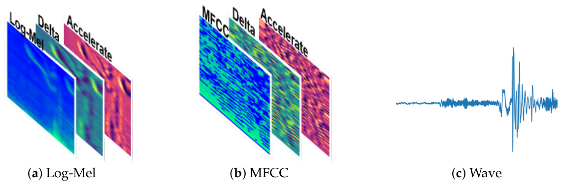
While the raw audio was recorded at 144 kHz, the fundamental frequencies of dolphin whistles lie primarily below 20 kHz. We therefore downsampled the data to 44.1 kHz using the Kaiser algorithm. The downsampled signals were then transformed into Log-Mel and MFCC spectrograms, and their first-order (delta) and second-order (accelerate) coefficients were added as additional channels. This results in three input representations: Log-Mel + delta + accelerate, MFCC + delta + accelerate, and raw waveform data, as illustrated in Figure 5.
Figure 5.
Input data formats. For the Log-Mel and MFCC inputs, the three color-coded layers represent the feature, Delta, and Acceleration coefficient components, respectively.
We used 64 Mel filter banks for the Log-Mel and MFCC transformation. The frame length was 80 ms and the frameshift is 10 ms. In such a case, the shape of the MFCC/Log-mel would be . In addition, we used a window size of 9 to calculate the delta and acceleration coefficients. This value is often used as a reasonable compromise between capturing sufficient temporal context and avoiding over-smoothing. It has been found to work well empirically in many audio processing tasks.
To evaluate model performance, we performed a 5-fold cross-validation. The dataset was divided into five stratified folds. In each of five iterations, four folds were used for training, while the remaining fold was split in half for validation and testing, resulting in an 8:1:1 ratio for training, validation and test sets.
2.3. Deep Learning Classification Methods
For whistle classification, we employed five widely used CNN network architectures [14], including MobileNet, Xception, ResNet, ResNeXt and SE-ResNeXt. MobileNet [21] is a lightweight CNN that uses depthwise separable convolutions to reduce computation complexity while maintaining strong performance, which is suitable for mobile applications. Xception [22] is the “Extreme Inception” model that decouples spatial and channel-wise convolutions for more efficient feature extraction. ResNet (Residual Network) [23] introduces residual connections (shortcuts) to enable effective training of very deep networks. ResNeXt [24] extends ResNet with grouped convolutions and a cardinality parameter, capturing a broader range of feature interactions. SE-ResNeXt [25] combines ResNeXt with Squeeze-and-Excitation blocks to model channel dependencies and enhance feature recalibration.
In the computer vision field, the input data typically consists of three 2-dimensional channels (red, green, and blue). In contrast, our mono-channel acoustic recordings are 1-dimensional time-series signals, making it difficult to apply standard vision-based CNN architectures directly. To ensure compatibility with these CNN models, we explored two types of feature representations for whistle signals, namely spectrogram-based representations and waveform-based representations.
For the spectrogram-based representations, the audio signal was first transformed into either a 2D log-scaled Mel spectrogram (Log-Mel) or a 2D Mel-frequency cepstral coefficient (MFCC) sequence. Both features are widely used in speech and sound recognition because they reflect human auditory perception. MFCCs characterize the short-term spectral envelope of the signal, while Log-Mel spectrograms provide a detailed time–frequency representation. To match the 3-channel input format of common CNNs, we then computed the first- and second-order delta coefficients for each feature map. These deltas capture temporal changes in the features, allowing the 3-channel representation to encode both the spectral structure and its evolution over time.
For the 1D waveform-based input, CNN architectures were adapted to directly accommodate raw audio. Specifically, a multi-scale stacking module is introduced to learn a 2D representation for the downstream 2D-convolutional layers, as shown in Table 2. The multi-scale stacking model ultimately connects to the first convolutional layer of the original model (reducing the number of input channels to 1). Unlike the Log-Mel or MFCC-based method, this module does not require explicit frequency-domain transformations. Instead, the convolutional blocks implicitly learn the spectral features, providing an end-to-end solution for the classification task.
Table 2.
Network architecture for waveform processing.
We trained the model from scratch for 50 epochs with the cross-entropy loss function and the stochastic gradient descent (SGD) optimizer. The initial learning rate was set to 0.01, and a cosine annealing schedule was adopted for learning rate adjustment. The model achieving the highest validation accuracy was retained for subsequent testing.
We further investigated fine-tuning ImageNet-pretrained CNN models [14] for the dolphin whistle classification task. The training dataset, methodology, model architectures and hyperparameters were kept identical to those used for models trained from scratch.
Mean average precision (mAP), a standard metric in information retrieval and object detection, was used to evaluate the models. It measures the average precision of a model across multiple classes. For each class, a precision–recall curve is computed, where precision (P) is defined as true positive (TP) divided by the sum of TP and false positive (FP), and recall (R) is the ratio of true positive detections to the total number of ground-truth positives. The average precision (AP) is calculated as the area under the interpolated precision–recall curve, and mAP is obtained by averaging the AP values across all classes or queries.
2.4. Simulation of Dolphin Whistle Signals
To further evaluate and enhance the robustness of the whistle classification models, we simulated whistle propagation through a marine acoustic channel and added in situ ambient noise at controlled SNR levels for both training and testing.
Specifically, we used BELLHOP to compute the impulse response of the marine acoustic channel between the source and the receiver. The simulated signals were then generated by convolving the whistle signal with this channel response:
where r(t) is the signal received from the receiver in simulation, r(t) is the source signal, and h(t) is the channel impulse response. To simplify the simulation model, it is assumed that the channel is linear and time invariant during the vocalization.
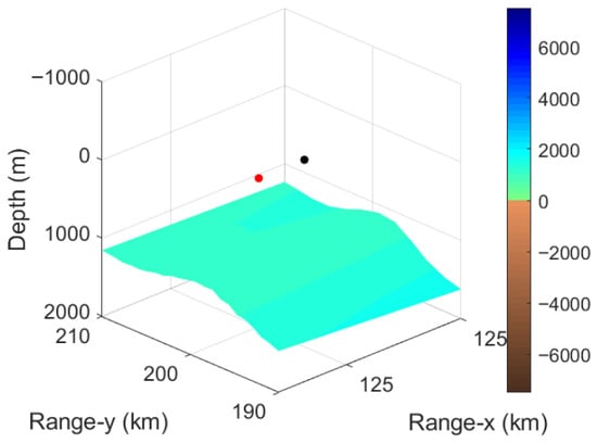
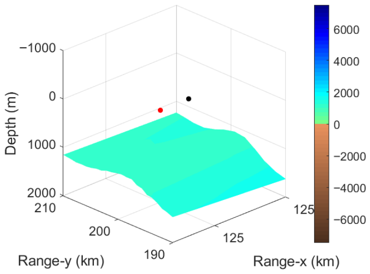
A standard environmental settings were used, including seabed topography, acoustic parameters, and the sound velocity profile. Both the source and receiver were positioned 100 m underwater to compute the acoustic channel impulse response, consistent with typical dolphin activity and hydrophone deployment. Figure 6 illustrates the locations of the source and receiver, along with the surrounding underwater terrain.
Figure 6.
Positions of the source (red) at 125 km, 200 km, and 100 m, and receiver (black) at 125.2 km, 200 km, and 100 m.
It should be noted that the underwater acoustic channel is complex, with multiple propagation paths generating many arrival pulses, most of which had very small amplitudes and minimal impact. For simplicity, pulses below 1% of the maximum amplitude were discarded. Additionally, because the impulse response was very weak, it was scaled by 100 to mimic the hydrophone gain and ensure a signal intensity comparable to the original. The cross-correlation analysis was then used to determine the offset introduced by convolution, ensuring that the simulated whistle signal was centered within the segment.
Figure 7 shows the spectrograms for one sample: original signal (left), its corresponding simulated signal (middle), and the difference between them (right).
Figure 7.
Spectrogram of the original slice (left), simulated slice (middle) and the difference value between them (right).
Ambient noise was assumed to be additive:
where y(t) denotes the resultant noisy signal, x(t) denotes the clean whistle signal, controls the noise intensity and n(t) is a noise signal randomly sampled from the ocean noise recordings in the SHIPSEAR dataset [26].
We assessed the robustness of the model on simulated datasets and further explored the potential of using simulated data for data augmentation. Altogether, the models were trained on three types of datasets from scratch: (1) original training data (org), (2) corresponding simulated training data (sim), and (3) a combination of original and simulated data (all). They were evaluated on the corresponding test sets: (1) original (org), (2) simulated (sim), and (3) combined (all), with varying SNR levels to assess model generalizability.
3. Results
3.1. Training from Scratch
Our analysis begins with an evaluation of all input feature representations across all models using the clean datasets. The results are summarized in Table 3. All three input representations, namely, Log-Mel (logmel), MFCC (mfcc), and the raw waveforms (wave), yielded strong performance, with every model achieving an mAP above 0.80. Although the waveform representation performed slightly below the MFCC and Log-Mel inputs across most architectures, the gap was modest. For example, the largest mAP difference between waveform and Log-Mel inputs was approximately 0.04 on the Xception model. Several factors may account for the performance advantage of spectrogram-based features. First, converting the waveform to a time–frequency representation can reduce the burden on the network to learn low-level spectral decomposition. Second, MFCC and Log-Mel features emphasize perceptually salient components, which may improve the training efficiency under limited data. In contrast, waveform-based models must learn these transformations implicitly, which often requires larger datasets or deeper architectures. In general, MFCC and Log-Mel inputs perform similarly. The highest mAP was achieved by the Xception architecture with the Log-Mel input, while the MFCC input lagged behind by only 0.01. This indicates that both representations are highly effective for whistle classification.
Table 3.
Class-level model performance on various input features.
In Table 3, we examined the class-level AP values. For each model, Log-Mel and MFCC demonstrated generally comparable performance across all categories. Interestingly, within the ResNet architecture, MFCC lagged behind Log-Mel by roughly 0.05 across the CV, SIN, and UP categories. And the waveform input in general could not perform well on CV and SIN classes. This degradation is likely influenced in part by the imbalanced class distribution.
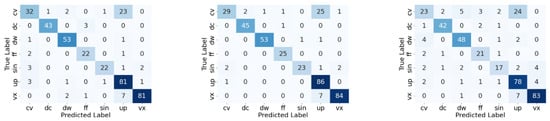
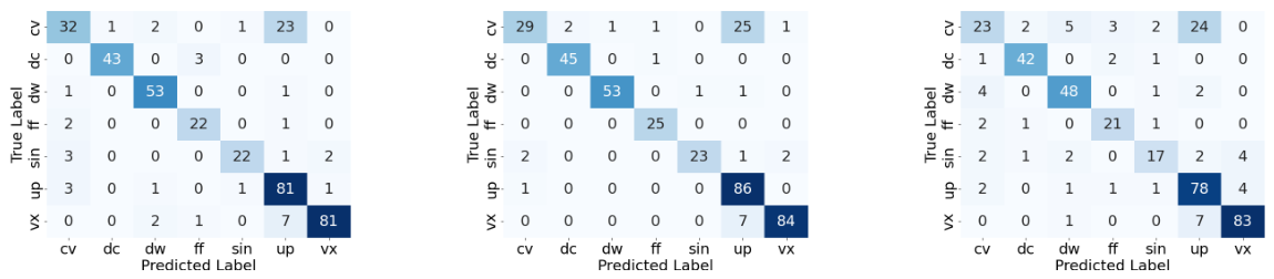
We further examined the confusion matrices (Figure 8) of the three input feature representations on the first fold of the best-performing Xception model. A large number of CV samples were misclassified as UP, leading to a reduced average precision for the CV class. This confusion is likely driven by the short duration of certain CV signals, causing models to interpret their rapid, transient frequency changes as resembling UP patterns. In contrast, the DC class—despite its limited sample size—showed more distinctive characteristics, as reflected in its consistently high AP scores. This observation indirectly supports the validity of the newly defined DC category, which is clearly separable from the six previously established classes.
Figure 8.
Confusion matrices of the Xception model on first-fold data using three input representations: Log-Mel (left), MFCC (middle), and Wave (right).
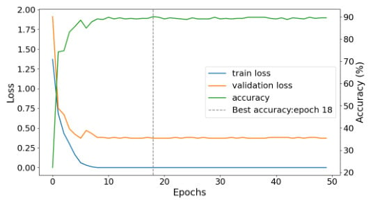
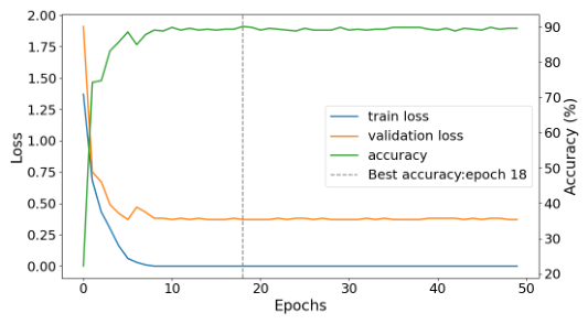
The best-performing training convergence process of the Xception model is illustrated in Figure 9. As the epoch increased, both training and validation losses decreased steadily and gradually converged, while the validation accuracy rose rapidly and tended to stabilize in the later stage. No obvious overfitting phenomenon was observed, demonstrating the rationality and stability of the training setup. The other models also achieved similar stable convergence patterns with only slight differences in convergence speed.
Figure 9.
Convergence behavior of the first-fold data in Log-Mel on the Xception model.
3.2. Fine-Tuning with Pretrained Weights
Table 4.
Class-level performance of fine-tuned pretrained models across input features.
Figure 10.
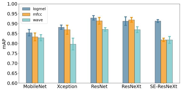
Comparison of fine-tuned pretrained model performance on various input features.
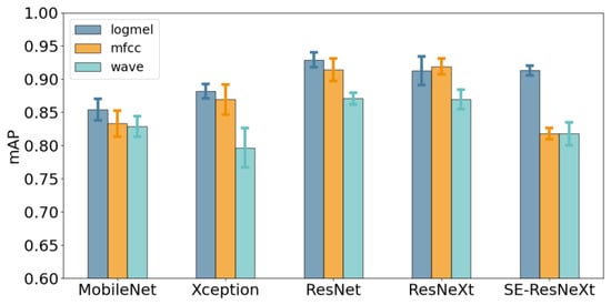
As shown in Figure 10, the ResNet-family models benefited from pretraining and fine-tuning, whereas models with fewer trainable parameters, such as MobileNet and Xception, showed no improvement. This advantage is likely due to the residual connections and larger model capacity in ResNet architectures, which facilitate more effective parameter updates and adaptation to new domains. It is also worth noting that the fine-tuned SE-ResNeXt performed poorly with MFCC inputs. This may be because MFCC processing generates a compact set of largely uncorrelated coefficients, whereas the pretrained SE modules are designed to capture channel correlations important for visual recognition. Since these learned channel relationships are not present in MFCC features, fine-tuning on them results in degraded performance. Conversely, starting from scratch to capture these MFCC features might yield better results than the original spectral features. Log-Mel features more closely resemble image-like representations, allowing the fine-tuned model to better leverage prior knowledge and achieve superior results. In contrast, models fine-tuned on waveform inputs showed smaller performance gains, because waveform data fundamentally differs from the other two spectral representations.
3.3. Model Robustness Testing and Enhancement Effects
The mAP results for model robustness testing and enhancement effects of Log-Mel, MFCC and waveform inputs are presented in Table 5, Table 6, and Table 7, respectively. Models trained on the original data with all three input types showed only a slight decrease in mAP (0.01–0.02) when evaluated on simulated data, indicating that they can still accurately classify the simulated signals. These results also suggest that, despite visual similarity on spectrograms, the simulated data introduce slightly more confusion in classification than the original recordings. When tested on signals with different SNR levels, models performed comparably to the clean dataset at high (40 dB, 30 dB) and moderate (20 dB) signal-to-noise ratio (SNR) levels. At lower SNRsS (10 dB), performance declined moderately but remains acceptable. When the SNR dropped to 0 dB, i.e., noise intensity matched the signal, model performance decreased sharply, as the noise overwhelmed the signal. Overall, all five models maintain adequate classification accuracy at SNRs of 10 dB or higher, suggesting potential applicability to real-world data. For lower-quality signals, further processing, such as signal enhancement, would be needed, though this is beyond the scope of the current study.
Table 5.
Model robustness on Log-Mel input.
Table 6.
Model robustness on MFCC input.
Table 7.
Model robustness on waveform input.
Table 5, Table 6 and Table 7 also indicate that incorporating simulated data generally improves mAP scores. The augmented training also enhances model robustness to noise, particularly at 0 dB SNR. Overall, these experiments demonstrate that the proposed data simulation process effectively improves model generalizability.
4. Discussion
Whistles serve as the primary communication tool for dolphins in their daily interactions. Analyzing whistle signals aids in understanding their behavioral patterns and social relationships, assists in assessing population dynamics, and facilitates conservation and monitoring efforts. From an audio signal perspective, the key distinctions among different whistles lie in their duration, frequency range, and modulation patterns. Research based on modulation patterns has led to preliminary classification of whistles [6,7,8]. By establishing such a classification system, we can further investigate the information conveyed by specific whistle types.
The first challenge we encountered was the limited sample size, inconsistent quality, and non-uniform labeling in the open datasets, which made data integration impractical. By conducting independent data collection and annotation, we resolved these issues. During this process, we repeatedly observed the composite concave structure classified as DC type—a feature previously overlooked by existing classification frameworks [6,7,8]. Although the definition of DC type remains flawed (e.g., lacking a scientifically established relationship between frequency and temporal spans), its clear distinguishability provides a heuristic guide to reconsider call modulation patterns from a novel perspective. Intuitively, among the six previous classifications, excluding the smooth FF type, if we interpret CV and VX as extensions of UP and DW—where CV = DW + UP and VX = VX + UP—could the SIN type be understood as a combination of CV and VX? SIN represents alternating sequences of these two types, and subdivided even further into CV followed by VX or vice versa. Our observations also revealed two identical combinations of basic types (i.e., DC, two CV instances). This leads us to consider whether the dolphin calls contain additional DV types combining two VX elements—a distinction we might have overlooked in earlier annotations. Alternatively, such advanced combinations may only emerge under more complex interaction scenarios, which have not yet been observed in our data. Interpreting the dolphin’s whistling in the same way we spell word combinations provides us with an extensive theoretical framework, opening up new avenues for a deeper understanding of this phenomenon.
The high discriminative power of the DC type demonstrates that deep learning models can capture subtle contour variations that might be overlooked by rule-based or manually parametrized approaches. Conversely, the persistent confusion between convex (CV) and upsweep (UP) whistles, particularly for short-duration signals, highlights a limitation of fixed-length input processing. Short convex whistles may have a rapid initial rise that mimics an upsweep when the descending portion is very brief. Future work could address this by employing attention mechanisms or variable-length sequence models, or by incorporating contextual information such as preceding and following vocalizations.
After obtaining the data, the next steps involve selecting the appropriate model and determining how to process the data. We adopted Xu et al.’s [14] method for generating 3D Log-Mel and MFCC spectra, but considering that Deyang [15] and Yang [16] preferred 1D audio inputs for end-to-end model deployment, we designed a multi-scale stacking module tailored for 2D waveform inputs. While its performance slightly lags behind spectrum-based approaches, it still demonstrates room for improvement. The choice of a 2D network stems from the fact that 1D raw audio is often lengthy; such networks require multiple layers and expanded receptive fields to model long-term dependencies, leading to higher parameter counts and computational demands. In contrast, converting audio to a 2D time–frequency spectrogram compresses the temporal dimension while preserving a local 2D structure, enabling the 2D network to effectively capture both long-term dependencies and time–frequency features with fewer layers and parameters. Consequently, under equivalent modeling performance, 2D time–frequency networks typically require fewer parameters than pure 1D audio networks.
Spectrum-based features and waveform-based transformations demonstrate superior overall performance in 2D convolutional neural networks (CNNs). When employing appropriate time–frequency representations, deep convolutional neural networks can classify the calls of the Indo-Pacific bottlenose dolphin with high accuracy. The optimal configuration—a fine-tuned ResNet model using LogMel input—achieved an average accuracy (mAP) of 0.929, significantly outperforming traditional feature-based manual classification methods, which typically achieve only 70% to 85% accuracy in similar contour recognition tasks [6,7,8,13]. This study demonstrates the feasibility of utilizing high-quality 2D convolutional networks for domain transfer classification of 1D audio and raises the question: Can 2D networks be applied to other domains (e.g., signal enhancement) for processing 1D audio data?
From a methodological perspective, the performance gap between training from scratch and fine-tuning ImageNet-pretrained weights reveals important considerations for bioacoustic deep learning. The ResNet family consistently benefited from transfer learning, while lightweight architectures like MobileNet did not, likely because their smaller capacity limits the advantage of reusing filters developed on natural images. Interestingly, fine-tuning SE-ResNeXt with MFCC inputs degraded performance dramatically, whereas Log-Mel fine-tuning succeeded. This disparity is likely due to the channel-wise feature recalibration in SE blocks, which assumes strong inter-channel correlations typical of RGB images. MFCC coefficients, by design, are largely decorrelated, making it difficult for the pretrained SE modules to adapt. This finding suggests that when using MFCC features, it may be preferable to either train from scratch or employ architectures without channel-attention mechanisms unless domain-specific pretraining is available. It also underscores the value of bioacoustics-specific self-supervised pretraining, an area that is gaining traction in animal vocalization studies [27,28].
The robustness experiments using BELLHOP-simulated propagation and additive ocean noise confirm that our models are not merely overfitting to the clean, captive-environment recordings. The models exhibited only a marginal drop in mAP when evaluated on simulated channel-affected whistles, and they maintained reliable performance down to SNR levels of 10 dB. These are encouraging results for field applications, where multipath propagation and variable background noise are the norm. More importantly, augmenting the training set with simulated data consistently improved both clean and noisy test performance, demonstrating that physically grounded data augmentation is an effective strategy for bridging the gap between controlled and real-world acoustic conditions. Using BELLHOP simulation data for data augmentation more closely resembles a hybrid approach of traditional methods like Mixup employed by [14], demonstrating another methodology for data enhancement. However, several caveats must be acknowledged. The BELLHOP simulation assumed a static, linear time invariant channel and a single source receiver geometry; real ocean channels exhibit time varying Doppler shifts, surface scattering, and biological noise sources that were not modeled. The SHIPSEAR noise samples, while representative of shipping noise, may not capture the full diversity of coastal habitats where Tursiops aduncus is found. Therefore, the reported robustness should be interpreted as a lower-bound estimate, and further validation on in situ recordings is necessary before operational deployment.
The ecological and conservation implications of automated whistle classification are significant. Tursiops aduncus is listed as a Class II protected species in China, and its coastal habitats are increasingly exposed to anthropogenic pressures such as shipping, construction, and fishing [11]. Passive acoustic monitoring (PAM) using autonomous recorders has become a cornerstone of cetacean conservation, yet the analysis of the resulting massive datasets remains a bottleneck [18,19]. The high accuracy and robustness demonstrated here suggest that CNN-based classifiers can be integrated into PAM workflows to automatically extract whistle type information, enabling long-term, large-scale monitoring of dolphin presence, behavioral states, and changes in vocal repertoire. For instance, shifts in the proportion of certain whistle contours could indicate disturbance responses or alterations in group composition [6,29]. Moreover, as signature whistles are known to carry individual identity information [9,10], future extensions of this work that combine contour classification with individual identification could provide fine-grained insights into population dynamics, social structure, and site fidelity—all critical parameters for conservation management.
Several limitations of the present study must be taken into account when interpreting the results. First, the dataset was collected from a single captive group of only five individuals (two adults and three infants) in a large but controlled pool environment. The acoustic repertoire of captive dolphins may differ from that of wild conspecifics in terms of whistle diversity, usage rates, and acoustic characteristics due to environmental and social differences [17]. Consequently, the seven whistle types identified here, including the new double concave class, may not encompass the full range of contours produced by wild Tursiops aduncus populations, and the class distribution observed may not reflect natural occurrence frequencies. Second, the dataset exhibits class imbalance, with some categories (e.g., constant, sine) having substantially fewer samples than others (e.g., convex). Although the models still achieved acceptable performance on the smaller classes, the imbalance likely contributed to the reduced AP for constant and sine whistles in certain configurations. Techniques such as weighted loss functions, oversampling, or data augmentation could be employed in future work to mitigate this issue. Third, the manual annotation process, while performed by experienced experts, introduces a degree of subjectivity, especially for whistles with ambiguous or transitional contours. Inter-annotator agreement was not formally quantified, and some samples assigned to one contour type may share features with another (as evidenced by the CV–UP confusion). Future dataset expansions should incorporate multi-annotator consensus and quantitative measures of contour similarity to refine category boundaries. Fourth, although the simulation-based augmentation improved robustness, the simulated signals are inherently simplified approximations. A promising direction is to combine physically based simulations with generative adversarial networks (GANs) or domain adaptation techniques to produce more realistic field-like training data.
Overall, this study provides a comprehensive benchmark for deep learning-based dolphin whistle classification and demonstrates that CNNs can effectively bridge the gap between clean, annotated datasets and challenging underwater acoustic environments. The findings support the feasibility of deploying automated classifiers in passive acoustic monitoring programs, with potential applications in behavioral ecology and conservation. Future work will focus on developing efficient detection-and-classification pipelines that can process continuous recordings in real time, exploring lightweight models for embedded systems on autonomous underwater vehicles or moored buoys, and extending the approach to other delphinid species and mixed-species assemblages. Additionally, combining whistle classification with localization and individual tracking could open new avenues for studying the communicative functions of different whistle types in natural contexts.
5. Conclusions and Future Work
This work presents a novel Tursiops aduncus whistles dataset, consisting of 3913 manually annotated signals across seven whistle types. Using this dataset, we develop a comprehensive framework to train and evaluate various CNN architectures and input feature representations. The experiments demonstrate that both the training-from-scratch model and the fine-tuned ImageNet-pretrained models achieve strong performance, with mAP consistently above 0.8. Xception performs best from scratch using Log-Mel and MFCC features, while pretrained ResNet-family models deliver comparable or slightly better accuracy. To assess the robustness of the models in a complex environment, we introduce simulated data generated with the BELLHOP acoustic channel and added real marine noise from the SHIPSEAR dataset. The models maintain reliable performance on simulated data and remain effective under moderate noise. Training with simulated data further improves accuracy and noise robustness, demonstrating its value as a practical augmentation strategy for whistle signal classification. Future work will focus on efficient dolphin signal detection methods and lightweight classification models suitable for deployment on resource-limited devices.
Author Contributions
M.X.: Conceptualization, Methodology, Data collection, Data curation, Software, Formal analysis, Writing—original draft. L.W.: Conceptualization, Methodology, Data curation, Software, Formal analysis, Writing—original draft. Y.C.: Conceptualization, Data collection, Data curation, Conceptualization, Funding acquisition, Project administration, Writing—review & editing. K.L.: Conceptualization, Data collection, Data curation, Formal analysis, Writing—original draft. Z.Z.: Conceptualization, Formal analysis, Funding acquisition, Project administration, Supervision, Writing—review & editing. J.C.: Investigation, Formal analysis, Supervision, Writing—review & editing. All authors have read and agreed to the published version of the manuscript.
Funding
This research was funded by Key Laboratory of Marine Environmental Survey Technology and Application, Ministry of Natural Resources, P. R. China, grant number MESTA-2023-A001 and National Natural Science Foundation of China under Grants 62301442, 62201164, 62192713.
Data Availability Statement
The data presented in this study are available on request from the corresponding authors.
Acknowledgments
We would like to express our sincere gratitude to Chimelong Ocean Kingdom for their generous support in collecting dolphin acoustic signals. Their assistance has been invaluable to this study. We also thank Jingwen Pang and Kefei Zhu for their efforts in the data annotation process.
Conflicts of Interest
The authors declare no conflict of interest.
References
- Au, W. Echolocation signals of wild dolphins. Acoust. Phys. 2004, 50, 454–462. [Google Scholar] [CrossRef] [Scilit]
- Au, W.W. The Sonar of Dolphins; Springer Science & Business Media: Berlin/Heidelberg, Germany, 1993. [Google Scholar]
- Herzing, D.L. Clicks, whistles and pulses: Passive and active signal use in dolphin communication. Acta Astronaut. 2014, 105, 534–537. [Google Scholar] [CrossRef] [Scilit]
- Janik, V.M.; Sayigh, L.S. Communication in bottlenose dolphins: 50 years of signature whistle research. J. Comp. Physiol. 2013, 199, 479–489. [Google Scholar] [CrossRef] [Scilit]
- Martin, M.J.; Elwen, S.H.; Kassanjee, R.; Gridley, T. To buzz or burst-pulse? The functional role of Heaviside’s dolphin, Cephalorhynchus heavisidii, rapidly pulsed signals. Anim. Behav. 2019, 150, 273–284. [Google Scholar] [CrossRef] [Scilit]
- Hawkins, E.R.; Gartside, D.F. Whistle emissions of Indo-Pacific bottlenose dolphins (Tursiops aduncus) differ with group composition and surface behaviors. J. Acoust. Soc. Am. 2010, 127, 2652–2663. [Google Scholar] [CrossRef] [Scilit] [PubMed]
- Azevedo, A.F.; Flach, L.; Bisi, T.L.; Andrade, L.G.; Dorneles, P.R.; Lailson-Brito, J. Whistles emitted by Atlantic spotted dolphins (Stenella frontalis) in southeastern Brazil. J. Acoust. Soc. Am. 2010, 127, 2646–2651. [Google Scholar] [CrossRef] [Scilit]
- Xue, R.; Niu, F.; Yang, Y.; Huang, Y.; Liu, W. Study on automatic extraction of bottlenose dolphin whistles from the background of ocean noise. In Proceedings of the 2nd International Conference on Information, Communication and Engineering, Nagoya, Japan, 12–15 April 2019. [Google Scholar]
- Janik, V.M.; Slater, P.J. Context-specific use suggests that bottlenose dolphin signature whistles are cohesion calls. Anim. Behav. 1998, 56, 829–838. [Google Scholar] [CrossRef] [Scilit]
- Harley, H.E. Whistle discrimination and categorization by the Atlantic bottlenose dolphin (Tursiops truncatus): A review of the signature whistle framework and a perceptual test. Behav. Process. 2008, 77, 243–268. [Google Scholar] [CrossRef] [Scilit]
- Haughey, R.; Hunt, T.N.; Hanf, D.; Passadore, C.; Baring, R.; Parra, G.J. Distribution and habitat preferences of Indo-Pacific bottlenose dolphins (Tursiops aduncus) inhabiting coastal waters with mixed levels of protection. Front. Mar. Sci. 2021, 8, 617518. [Google Scholar] [CrossRef] [Scilit]
- Matthews, J.; Rendell, L.E.; Gordon, J.C.D.; Macdonald, D. A review of frequency and time parameters of cetacean tonal calls. Bioacoustics 1999, 10, 47–71. [Google Scholar] [CrossRef] [Scilit]
- McCowan, B. A new quantitative technique for categorizing whistles using simulated signals and whistles from captive bottlenose dolphins (Delphinidae, Tursiops truncatus). Ethology 1995, 100, 177–193. [Google Scholar] [CrossRef] [Scilit]
- Xu, K.; Zhu, B.; Kong, Q.; Mi, H.; Ding, B.; Wang, D.; Wang, H. General audio tagging with ensembling convolutional neural networks and statistical features. J. Acoust. Soc. Am. 2019, 145, EL521–EL527. [Google Scholar] [CrossRef] [Scilit]
- Gao, D.; Gao, D.; Li, X. Deep learning-based recognition of click signals of typical marine mammals. J. Shaanxi Norm. Univ. Sci. Ed. 2019, 47, 37–437. [Google Scholar]
- Yang, W.; Luo, W.; Zhang, Y. Classification of odontocete echolocation clicks using convolutional neural network. J. Acoust. Soc. Am. 2020, 147, 49–55. [Google Scholar] [CrossRef] [Scilit]
- Sayigh, L.S.; Janik, V.M.; Jensen, F.H.; Scott, M.D.; Tyack, P.L.; Wells, R.S. The Sarasota Dolphin Whistle Database: A unique long-term resource for understanding dolphin communication. Front. Mar. Sci. 2022, 9, 923046. [Google Scholar] [CrossRef] [Scilit]
- Di Nardo, F.; De Marco, R.; Lucchetti, A.; Scaradozzi, D. A WAV file dataset of bottlenose dolphin whistles, clicks, and pulse sounds during trawling interactions. Sci. Data 2023, 10, 650. [Google Scholar] [CrossRef] [Scilit] [PubMed]
- Wall, C.C.; Haver, S.M.; Hatch, L.T.; Miksis-Olds, J.; Bochenek, R.; Dziak, R.P.; Gedamke, J. The next wave of passive acoustic data management: How centralized access can enhance science. Front. Mar. Sci. 2021, 8, 703682. [Google Scholar] [CrossRef] [Scilit]
- Porter, M.B.; Bucker, H.P. Gaussian beam tracing for computing ocean acoustic fields. J. Acoust. Soc. Am. 1987, 82, 1349–1359. [Google Scholar] [CrossRef] [Scilit]
- Howard, A.G. Mobilenets: Efficient convolutional neural networks for mobile vision applications. arXiv 2017, arXiv:1704.04861. [Google Scholar] [CrossRef] [Scilit]
- Chollet, F. Xception: Deep learning with depthwise separable convolutions. In Proceedings of the IEEE Conference on Computer Vision and Pattern Recognition, Honolulu, HI, USA, 21–26 July 2017; pp. 1251–1258. [Google Scholar]
- He, K.; Zhang, X.; Ren, S.; Sun, J. Deep residual learning for image recognition. In Proceedings of the IEEE Conference on Computer Vision and Pattern Recognition, Las Vegas, NV, USA, 27–30 June 2016; pp. 770–778. [Google Scholar]
- Xie, S.; Girshick, R.; Dollár, P.; Tu, Z.; He, K. Aggregated residual transformations for deep neural networks. In Proceedings of the IEEE Conference on Computer Vision and Pattern Recognition, Honolulu, HI, USA, 21–26 July 2017; pp. 1492–1500. [Google Scholar]
- Hu, J.; Shen, L.; Sun, G. Squeeze-and-excitation networks. In Proceedings of the IEEE Conference on Computer Vision and Pattern Recognition, Salt Lake City, UT, USA, 28–23 June 2018; pp. 7132–7141. [Google Scholar]
- Santos-Domínguez, L.; Vázquez, M.; Llorca, J.M.; Carballo, A. ShipsEar: An underwater vessel noise database. Appl. Acoust. 2016, 114, 155–163. [Google Scholar] [CrossRef] [Scilit]
- Stowell, D.; Wood, M.; Pamuła, H.; Stylianou, Y.; Glotin, H. Automatic acoustic detection of birds through deep learning: The first Bird Audio Detection challenge. Methods Ecol. Evol. 2019, 10, 368–380. [Google Scholar] [CrossRef] [Scilit]
- Bermant, P.; Bronstein, M.; Wood, R.; Gero, S.; Gruber, D. Deep machine learning techniques for the detection and classification of sperm whale bioacoustics. Sci. Rep. 2019, 9, 12588. [Google Scholar] [CrossRef] [Scilit] [PubMed]
- Oswald, J.N.; Barlow, J.; Lammers, M.O. Acoustic identification of nine delphinid species in the eastern tropical Pacific Ocean. Mar. Mammal Sci. 2007, 23, 20–37. [Google Scholar] [CrossRef] [Scilit]



Disclaimer/Publisher’s Note: The statements, opinions and data contained in all publications are solely those of the individual author(s) and contributor(s) and not of MDPI and/or the editor(s). MDPI and/or the editor(s) disclaim responsibility for any injury to people or property resulting from any ideas, methods, instructions or products referred to in the content. |
© 2026 by the authors. Licensee MDPI, Basel, Switzerland. This article is an open access article distributed under the terms and conditions of the Creative Commons Attribution (CC BY) license.