Ship Equipment Order Target Price Prediction: An Interpretable Model Based on Boruta–Lasso and CatBoost-SHAP

Abstract

The target price for naval equipment orders is driven by the coupling of multidimensional technical and economic factors, exhibiting typical characteristics such as high dimensionality, strong nonlinearity, multicollinearity, and small-sample fluctuations. Traditional cost estimation methods struggle to achieve high-precision fitting and interpretable decision support. To address these issues, this paper constructs an integrated prediction model that combines Boruta–Lasso two-stage feature selection, grid search-optimized CatBoost, and SHAP interpretability analysis. First, the Boruta algorithm is used for rough screening of feature significance, then Lasso regression is applied for sparse fine screening, effectively eliminating redundant features and significantly mitigating multicollinearity; grid search and five-fold repeated cross-validation are employed to optimize CatBoost hyperparameters, while 10 repeated experiments with random seeds are conducted to verify model generalization robustness. SHAP is used to quantify the marginal contribution of features, revealing nonlinear associations and statistical response transition points between core features and price. This study is based on 33 publicly available real data from main combat vessels, from which 198 modeling samples were generated through interpolation-based small-sample data augmentation. The interpolated samples were only used for data augmentation and were not considered independent empirical samples. All core conclusions were validated on the 33 original real samples, and there are no missing values in the dataset. Experimental results show that the proposed model achieved the best individual results on the test set, with a coefficient of determination of R² = 0.8949, root mean square error RMSE = 0.0554, and mean absolute error MAE = 0.0476. Across 10 repeated robustness experiments, the average results were R² = 0.8828, RMSE = 0.0586, and MAE = 0.0529, with overall performance better than comparison models such as XGBoost, random forest, and standard CatBoost. Ablation experiments validated the effectiveness of the two-stage Boruta–Lasso selection strategy in improving model accuracy and stability. SHAP attribution analysis shows that full-load displacement, number of vertical missile launch cells, number of phased array radars, and combat capability are core features highly correlated with price, all showing significant nonlinear positive correlations and clear statistical response transition points. The dataset in this study has no missing values, is entirely constructed based on publicly traceable data, and does not include confidential information such as internal shipyard costs. The findings reflect statistical associations rather than causal effects. However, the sample size and ship-type coverage are limited, so the model’s applicability is somewhat constrained, and its generalization ability needs to be further verified on larger-scale, multi-ship-type independent datasets. This model combines high prediction accuracy, strong robustness, and good interpretability, providing reliable technical support for ship equipment procurement pricing demonstration, full lifecycle cost management, and scientific procurement decision-making.

1. Introduction

The target price for ship equipment orders is the core basis for the preparation of ship equipment procurement budgets, pricing demonstrations, and cost control. Its formation is influenced by multiple coupled factors [1], such as ship equipment displacement, main dimensions, power systems, weapon configurations, electronic equipment, and comprehensive combat effectiveness, exhibiting typical characteristics of high dimensionality, strong nonlinearity, multiple collinearity, and small-sample fluctuations [2]. Traditional cost estimation methods based on engineering parameter methods, linear regression, or gray models struggle to capture complex nonlinear relationships. The lifecycle cost (LCC) of a ship is affected by the coupled impacts of multiple stages, including design, construction, and operation and maintenance, while the lack of systematic feature selection results in insufficient prediction accuracy and weak generalization capability. This makes it difficult to meet the modern equipment pricing management requirements of being ‘scientific, traceable, and interpretable’ and cannot provide stable and reliable technical support for procurement budget preparation, price verification, and cost optimization [3,4,5].

From the existing literature, research on ship cost prediction has produced three typical outcomes: First, traditional methods represented by parametric estimation, linear regression, and gray models, which have simple structures but cannot characterize complex nonlinear relationships and are insufficiently accurate in high-dimensional scenarios; second, ensemble learning methods represented by random forest and XGBoost, which show improved prediction performance but generally do not conduct systematic feature selection and are prone to multicollinearity and overfitting; third, a small number of studies that combine feature selection and predictive models, but they mostly use a single-selection strategy, are unable to balance feature completeness and sparsity, and have weak model interpretability, making it difficult to support traceable pricing decisions. Existing research has yet to form an integrated framework combining ‘two-stage feature selection—optimized ensemble prediction—interpretability analysis,’ and significant gaps remain in methodological systems, empirical support, and engineering applications.

Feature selection is a key preprocessing step for mitigating high-dimensional redundancy, suppressing collinearity, and improving model stability. The Boruta algorithm can retain features relevant to the target [6], while Lasso regression can achieve sparse selection and compress feature dimensions [7]. Combining the two can implement a two-stage complementary framework of ‘coarse screening of significant features—refined sparse screening.’ This approach has already achieved good application results in fields such as medical diagnosis and energy demand forecasting [8,9,10,11,12]. In terms of predictive models, CatBoost has advantages in handling categorical features, suppressing gradient bias, and preventing overfitting, and it is commonly applied in scenarios with small samples, nonlinearity, and multi-source heterogeneous data [13,14,15]. The SHAP interpretability method can quantify feature contributions and reveal decision logic, effectively addressing the ‘black box’ problem in machine learning, and has become a standard tool for model interpretability analysis [16,17,18,19]. Although the above methods are relatively mature, there is still a lack of systematic integration and validation in the field of ship order target price prediction. No study has yet combined Boruta–Lasso two-stage screening, GridSearchCV-optimized CatBoost, and SHAP interpretability analysis to form a practical, high-precision, and interpretable pricing prediction tool.

To this end, this paper constructs a ship order target price prediction model based on Boruta–Lasso feature selection and CatBoost-SHAP. First, Boruta is used to perform full-feature significance screening; then, Lasso is applied for sparsification and collinearity suppression to obtain a stable core feature set. Subsequently, CatBoost is optimized via grid search to achieve high-precision nonlinear fitting. Finally, SHAP is used to reveal the statistical associations and nonlinear response patterns between key features and prices. Experimental results show that the model achieves a coefficient of determination R² of 0.8949, an RMSE of 0.0554, and an MAE of 0.0476, demonstrating excellent performance and high prediction accuracy on this dataset. Ablation experiments confirm that the two-stage feature selection effectively enhances model stability. SHAP analysis indicates that ship equipment full-load displacement, the number of missile vertical launch units, the number of phased array radars, and combat power of equipment are core features highly statistically associated with price, all showing significant nonlinear positive correlations. This study provides a high-precision, interpretable, and practical prediction method for ship equipment ordering prices, offering strong support for equipment cost control, pricing demonstration, and scientific decision-making.

The rest of this paper is organized as follows. Section 2 is a literature review. Section 3 introduces the research methods of this paper. Section 4 conducts simulation experiments and discusses the research results. Section 5 draws the conclusions.

2. Literature Review

2.1. Current Status of Research on Ship Equipment Cost and Price Prediction

The target price for ordering naval equipment is influenced by multiple factors, such as tonnage scale, power configuration, weapon and electronic systems, construction technology, and the procurement environment, exhibiting characteristics of high dimensionality, strong nonlinearity, small-sample fluctuations, and multicollinearity. It has long been a challenging area in the field of equipment pricing and cost control. Early studies mostly relied on traditional parametric methods, linear regression, and gray system models to estimate costs and maintenance fees [20,21,22,23,24,25,26,27,28,29,30,31]. Internationally, a full lifecycle cost analysis framework for ship structure, operation, and maintenance has been established, and a standardized shipbuilding cost estimation system has gradually formed. Such methods are structurally intuitive and easy to apply in engineering, but they struggle to capture multi-feature interactions and complex nonlinear patterns. In high-dimensional feature scenarios, their accuracy is limited, making it difficult to support refined pricing requirements.

With the popularization of machine learning and ensemble learning methods, models such as random forest and XGBoost have gradually been introduced into the prediction of ship construction costs, repair costs, and lifecycle expenses [32,33,34,35], and related methods have been widely validated in the field of marine engineering, such as in JMSE [36,37,38,39,40,41,42,43]. Compared with traditional methods, they have improved fitting accuracy. However, existing research on ship price prediction still has obvious limitations: most studies directly use the full set of features for modeling, lacking a targeted high-dimensional feature selection process. The models are easily affected by redundant features and multicollinearity, resulting in insufficient generalization performance and stability. Meanwhile, most current results focus on improving prediction accuracy, paying insufficient attention to the interpretability of model decision mechanisms, making it difficult to meet the management requirements of equipment pricing being “traceable, auditable, and explainable”. In addition, there is a lack of empirical analysis of the marginal effects of key features, nonlinear variation patterns, and statistical response transition points, which cannot provide a quantitative basis for equipment configuration optimization and cost control.

2.2. Progress in Feature Selection Methods for High-Dimensional Data

The factors affecting ship prices are high-dimensional and highly correlated, and redundant and noisy features can significantly reduce model efficiency and exacerbate overfitting. Therefore, feature selection is a critical step in the modeling process. Traditional feature selection methods mainly include filter methods, wrapper methods, and embedded methods. Among them, filter methods are computationally efficient but ignore interactions between features; wrapper methods have higher accuracy but incur high computational cost; embedded methods can perform feature selection synchronously during training, but they cannot easily guarantee the completeness of important features.

In recent years, two-stage combined feature screening has become a mainstream approach for high-dimensional data modeling, balancing feature completeness and sparsity. The Boruta algorithm, based on random forests and shadow features, performs significance testing and can retain as many important features related to the target as possible. Lasso implements sparsity selection based on L1 regularization, which can effectively compress redundant features and alleviate multicollinearity. The combined use of the two forms a “significance coarse screening—sparsity fine screening” strategy, which has been validated in fields such as energy and healthcare. However, in the context of ship equipment price prediction, there is still a lack of systematic application and comparative validation [44]. How to adapt to the small-sample, highly coupled characteristics of ship data and form a stable and efficient feature selection process remains an urgent issue to be addressed.

2.3. Research Status of Integrated Prediction and Interpretability Methods

In the field of nonlinear predictive modeling, CatBoost demonstrates stable performance in small-sample, highly heterogeneous, and strongly nonlinear regression tasks because it can automatically handle categorical features and suppress gradient bias and overfitting. This makes it more suitable for the characteristics of ship equipment price data, and it has already been applied to ship economic assessments and lifecycle cost optimization, showing good robustness in complex engineering regression tasks [45,46,47]. In terms of model interpretability, the SHAP method realizes unified feature contribution quantification based on game theory, supporting both global and local explanations. It has become a standard tool for interpretable analysis of tree models and can effectively address the “black box” problem in machine learning. It has been widely used in decision analysis across various regression tasks [48,49,50,51,52]. Existing studies have attempted to combine feature selection, ensemble models, and SHAP, but a complete research framework targeting the ordering price of ships has not yet been formed. On one hand, there is a lack of deep integration of two-stage feature screening and optimized predictive modeling specifically for ship price scenarios; on the other hand, the lack of systematic revelation of patterns such as nonlinear dependence on key features, changes in marginal effects, and statistical response transition points makes it difficult for interpretable results to directly support pricing decisions and program optimization.

2.4. Aspects of Existing Research That Need Further Improvement

Overall, there are still four prominent shortcomings in the field of target price prediction for ship equipment procurement: (1) high-dimensional features lack a two-stage screening strategy adapted to ship data characteristics, resulting in insufficient model stability and generalization ability; (2) the prediction model has a prominent “black box” problem, and its interpretability cannot meet the management requirements for equipment pricing review and decision traceability; (3) there is a lack of empirical analysis on the nonlinear statistical correlation between key features and prices, marginal response patterns, and statistical response transition points; and (4) an integrated, practical pricing prediction support system of “efficient feature screening—optimized predictive modeling—interpretability analysis” has not yet been formed. To address this, this paper introduces Boruta–Lasso two-stage feature selection, grid-optimized CatBoost, and SHAP interpretability analysis to construct an integrated predictive model, specifically filling the existing research gaps and providing a more accurate, stable, and interpretable technical method for ship equipment procurement pricing.

3. Method

This chapter clearly divides the modeling process into six standardized steps: data preprocessing, feature selection, model training, hyperparameter tuning, final testing, and interpretability analysis. It also provides unified mathematical symbols, standardized formulas, and algorithm pseudocode to ensure that the process is reproducible.

3.1. Symbol Definition

Suppose the original dataset contains $N$ samples and $D$ features. Denote: the original feature matrix as $X\in R^{N\times D}$, the target price vector as $y\in R^N$, the training set as $X_{train}\in R^{N_{train}\times D}$, $y_{train}\in R^{N_{train}}$, the test set as $X_{test}\in R^{N_{test}\times D}$, $y_{test}\in R^{N_{test}}$, and the reduced feature set after feature selection as $X_{sel}\in R^{N\times d}(d\ll D)$.

3.2. Data Preprocessing

Data preprocessing is a key step for eliminating differences in dimensions, standardizing data distribution, and ensuring modeling compliance. All operations are completed before feature selection and model training, and all standardization statistics are calculated only from the training set to strictly avoid data leakage.

3.2.1. Min–Max Normalization

The dimensional differences in ship equipment characteristics are significant (such as displacement, power, quantity, and days), and direct modeling will cause the model to be overly sensitive to features with large values. Therefore, min–max normalization is used to linearly map all features to the [0, 1] range, and the conversion formula is:

$${x^{\prime }}_{ij}={\displaystyle \frac{x_{ij}-\min (x_j)}{\max (x_j)-\min (x_j)}}$$

(1)

In the formula: $x_{ij}$ is the original value of the $j$ dimension feature of the $i$ sample; $\min (x_j)$ and $\max (x_j)$ are the minimum and maximum values of the $j$ dimension feature in the training set, respectively; and ${x^{\prime }}_{ij}$ is the standardized feature value.

3.2.2. Handling Missing Values and Outliers

Both the original sample and the dataset expanded through interpolation in this study have no missing values, so there is no need for missing value imputation or sample deletion. Only the purchase prices were subjected to currency conversion and temporal deflation, converting them to constant 2024 prices to ensure comparability of sample prices across years and currencies.

3.2.3. Dataset Partitioning

After preprocessing, this study strictly follows the principles of three-layer isolation, no overlap, and no information leakage to construct the training set, validation set, and test set, ensuring unbiased model evaluation and reproducible procedures. Firstly, all 33 original real samples are divided into a real training set and an independent test set at a ratio of 8:2. The test set is completely sealed throughout and does not participate in feature selection, parameter tuning, or model training; it is only used for the final generalization performance evaluation. Secondly, the real training set is further divided into a real sub-training set and an independent validation set at an 87.5:12.5 ratio. The validation set is only used for hyperparameter optimization and does not participate in feature selection or model training. Finally, the interpolated augmented samples are combined with the real sub-training set to form the final training set for modeling.

In the end, three completely independent datasets are formed: the training set, composed of interpolated augmented data and the real sub-training set is used for feature selection and model training; the validation set, originating from real samples, is used exclusively for hyperparameter optimization; and the test set, consisting of independently isolated real samples, is used only for final unbiased evaluation. Throughout the entire process, feature selection, standardization, hyperparameter optimization, and SHAP global interpretation are all performed solely within the training set. The validation set and test set do not participate in any preliminary steps, mechanistically preventing data leakage and ensuring reliable and credible experimental results.

3.3. Feature Selection

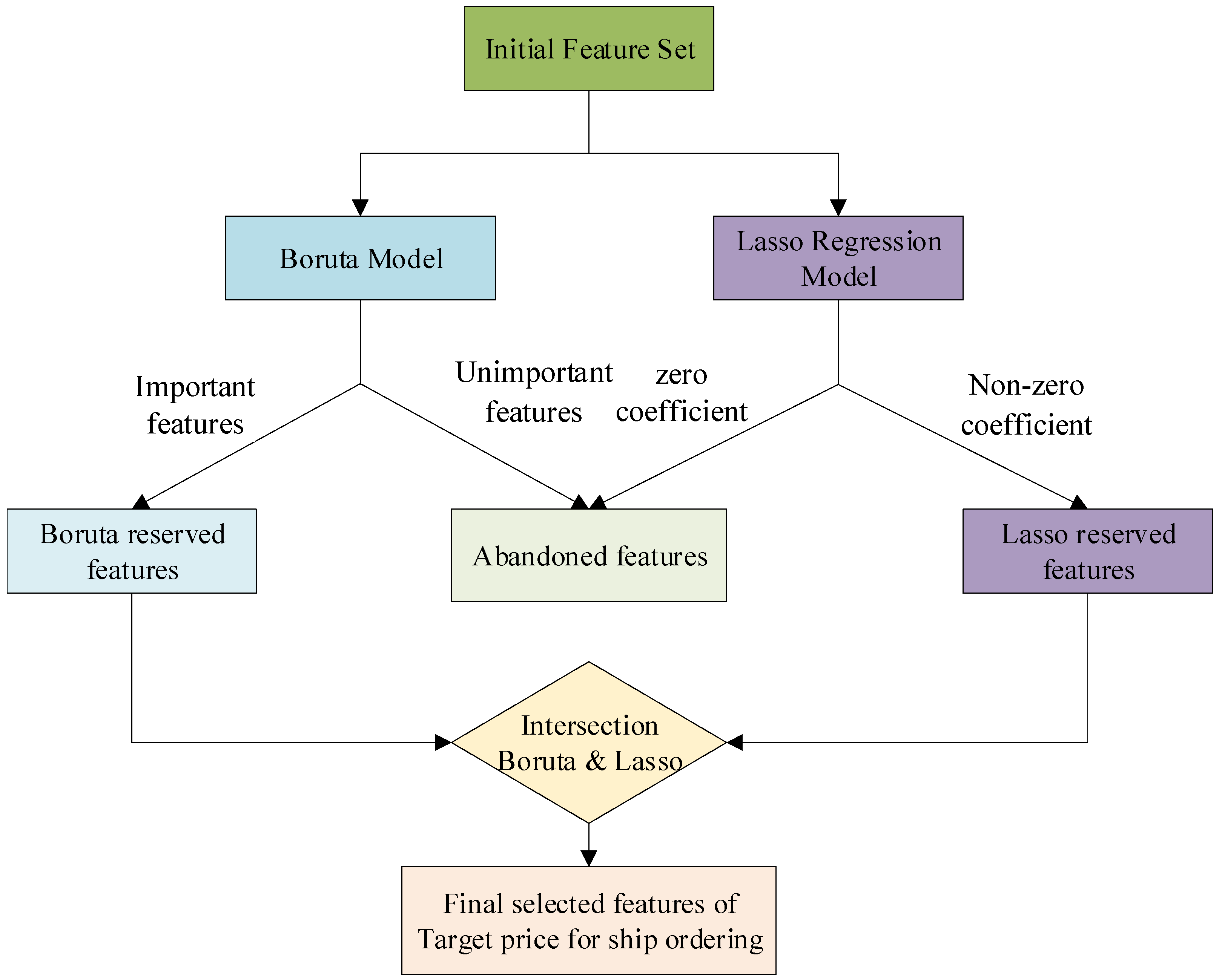
Considering the high dimensionality and strong multicollinearity of factors influencing ship price, a two-stage strategy combining Boruta significance-based coarse screening with Lasso sparsity-based fine screening is adopted, balancing feature completeness and sparsity. The two-stage feature selection process is performed independently only on the training set, while the test set directly reuses the feature subset obtained from the training set, without participating in any feature screening process, to avoid data leakage.

3.3.1. Boruta Feature Selection

Boruta performs significance testing based on random forests and shadow features and can retain all features related to the target statistic, avoiding the loss of critical engineering information. This method determines whether the importance of the original features is significantly higher than that of the randomly permuted shadow features as the basis for judgment and outputs a coarse-filtered feature set ${\mathcal{F}}_B$.

3.3.2. Lasso Regularization Sparse Selection

Lasso compresses the coefficients of redundant features to 0 through regularization $L_1$, achieving feature sparsity and alleviating multicollinearity. Its objective function is:

$$\widehat{\beta }=\arg \underset{\beta }{\min }\{{‖y-X\beta ‖}_2^2+\lambda {‖\beta ‖}_1\}$$

(2)

In the formula: ${‖y-X\beta ‖}_2^2$ is the fitting loss term; ${‖\beta ‖}_1$ is the regularization term $L_1$; and $\lambda$ is the regularization parameter used to control the sparsity level.

3.3.3. Final Feature Set Construction

To ensure feature stability, the intersection of the two-stage screening results is taken as the final feature set:

$${\mathcal{F}}_{final}={\mathcal{F}}_B\cap {\mathcal{F}}_L$$

(3)

Ultimately, a streamlined feature set was obtained that is statistically significant, significantly alleviates multicollinearity, and has clear engineering significance. To quantitatively assess feature multicollinearity, the variance inflation factor (VIF) was used for testing. After standardization, the full-feature dataset had an average VIF of 18.01 and a maximum VIF of 119.95, indicating obvious multicollinearity. After Boruta selection, the average VIF decreased to 11.05. After Lasso selection, the average VIF decreased to 8.27. Finally, after the two-stage Boruta–Lasso selection, the average VIF was 8.68, with a maximum VIF of 32.03. Compared with the original full-feature set, multicollinearity was significantly alleviated, meeting the modeling requirements. Figure 1 shows the complete process of this two-stage feature selection model.

3.4. CatBoost Model Training

A nonlinear prediction model is constructed using CatBoost gradient boosting decision trees, which have the advantages of automatically handling categorical features, suppressing gradient bias, and reducing overfitting, making them suitable for scenarios with small sample sizes and highly heterogeneous data in ship equipment. The model’s prediction function takes the form of a sum of multiple decision trees:

$$\widehat{y}(x)={\displaystyle \sum _{k=1}^K{f}_k(x)}$$

(4)

In the formula, $K$ represents the number of decision trees, and $f_k(x)$ represents the output of the $k$ tree. To control model complexity, the objective function simultaneously includes the fitting loss and double regularization terms:

$$L={\displaystyle {\displaystyle \sum _{i=1}^N}l(y_i,{\widehat{y}}_i)}+{\displaystyle {\displaystyle \sum _{k=1}^K}(\gamma T_k+\frac{1}{2}\lambda {‖{\omega }_k‖}^2)}$$

(5)

In the formula, $l(y_i,{\widehat{y}}_i)$ is the sample loss, $T_k$ is the number of leaf nodes of the $k$ tree; ${\omega }_k$ is the weight of the leaf nodes, and $\gamma$ and $\lambda$ are regularization coefficients used to control tree complexity and overfitting.

3.5. Hyperparameter Tuning

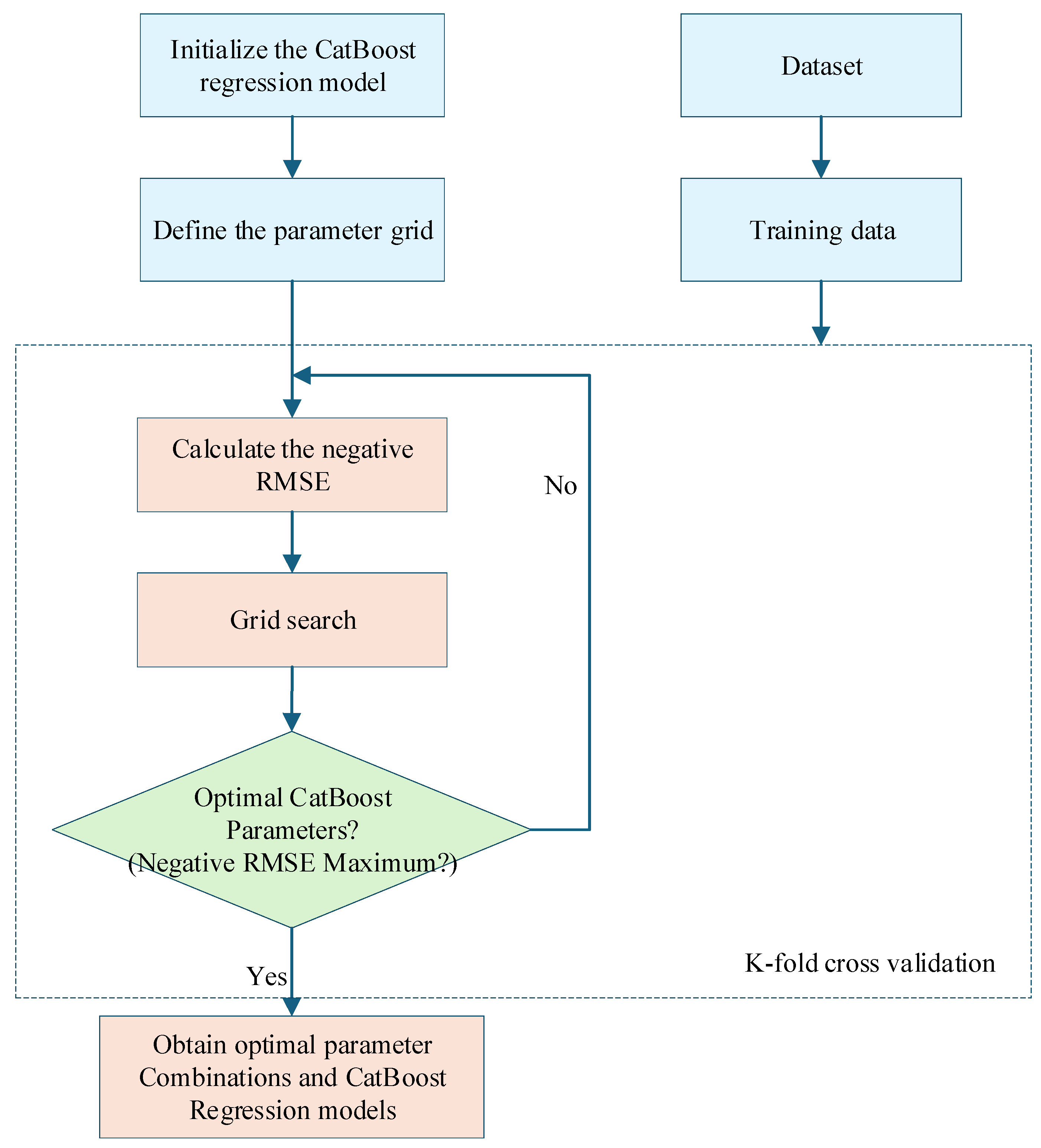
To adapt the model to ship price data, grid search (GridSearchCV) and five-fold, three-repeated cross-validation are used for automatic hyperparameter optimization. The entire process of grid search and cross-validation is conducted only within the training set, with the validation set split from the training set, and the test set does not participate in the tuning process at all. The optimized parameters include learning rate, number of iterations, and maximum tree depth. The tuning process uses only the training set and internal validation set, without introducing any information from the test set, strictly avoiding data leakage and ensuring unbiased evaluation results. The hyperparameter tuning process is shown in Figure 2.

3.6. Final Independent Test

After the model training is completed, three metrics are calculated on a completely independent test set to evaluate generalization performance.

3.6.1. Coefficient of Determination R²

$$R^2=1-{\displaystyle \frac{{\displaystyle {\sum }_{i=1}^{N_{test}}{(y_i-{\widehat{y}}_i)}^2}}{{\displaystyle {\sum }_{i=1}^{N_{test}}{(y_i-\overline{y})}^2}}}$$

(6)

This metric is used to measure the model’s ability to explain price variability; the closer the value is to one, the better the fit.

3.6.2. Root Mean Square Error (RMSE)

$$RMSE=\sqrt{{\displaystyle \frac{1}{N_{test}}}{\displaystyle \sum _{i=1}^{N_{test}}{(y_i-{\widehat{y}}_i)}^2}}$$

(7)

This metric reflects the average deviation between predicted values and actual values; the smaller the value, the higher the accuracy.

3.6.3. Mean Absolute Error (MAE)

$$MAE={\displaystyle \frac{1}{N_{test}}}{\displaystyle \sum _{i=1}^{N_{test}}\left|y_i-{\widehat{y}}_i\right|}$$

(8)

This metric is insensitive to outliers and robustly reflects the level of prediction error.

3.7. SHAP Interpretability Analysis

Using Tree-SHAP to attribute model decisions only reveals statistical association patterns and does not derive causal relationships. SHAP global explanations (feature importance, dependence plots, and statistical response transition point calculations), are all strictly based on the training set, with the test set used only for final predictions and local attribution display. Thes test set is not involved in any global explanation process, ensuring no data leakage and unbiased evaluation.

3.7.1. SHAP Value Calculation Formula

The contribution of feature j to the prediction result (Shapley value) is:

$${\varphi }_j={\displaystyle \sum _{S\subseteq M\backslash \left\{j\right\}}\frac{\left|S\right|!\cdot (\left|M\right|-\left|S\right|-1)!}{\left|M\right|!}\left[v(S\cup \{j\})-v(S)\right]}$$

(9)

In the formula, $M$ is the set of features, $S$ is the subset of features, $v(\cdot )$ is the model prediction output, and ${\varphi }_j$ is the marginal contribution of feature $j$.

3.7.2. Statistical Response Transition Point and Uncertainty Estimation

To identify the key transition point at which features affect price, LOWESS is applied to smooth the SHAP dependence scatter for each core feature. Using SHAP = 0 as the boundary, the intersection of the smoothed curve with the zero axis is found and recorded as the statistical response transition point. Then, 100 bootstrap resamplings are used to calculate the 95% confidence interval (95% CI) of the statistical response transition point, quantifying the uncertainty of the transition point estimate.

3.8. Overall Modeling Process and Pseudocode

The full-text modeling follows a unified process: preprocessing → data splitting → feature selection → hyperparameter tuning → model training → independent testing → SHAP interpretability analysis. The specific content is shown in Algorithm 1.

Algorithm 1: Ship Equipment Order Target Price Prediction Model

Input: Original feature matrix X, equipment price vector y Output: Optimal prediction model, core feature subset, SHAP statistical response transition point, and 95% confidence intervals 1. Data Preprocessing: Perform price deflation processing, outlier detection, and correction. 2. Three-layer strict dataset splitting: Following the principle of no sample overlap and complete isolation, completely preventing data leakage: 2.1 Divide the 33 original real samples into a real training set and an independent test set at an 8:2 ratio; the test set remains completely sealed and is not involved in feature selection, hyperparameter optimization, or model training, only used for final unbiased generalization performance evaluation. 2.2 Further split the real training set at an 87.5:12.5 ratio into a real sub-training set and an independent validation set; the validation set is only used for hyperparameter optimization, not for feature selection or model training. 2.3 Merge interpolated augmented samples with the real sub-training set to construct the final modeling training set. 3. Feature Standardization: Fit the min-max normalization rule only based on the final training set, then consistently transform the training set, validation set, and test set. 4. Two-stage Feature Selection: Execute Boruta–Lasso two-stage feature selection only within the final training set to identify the core feature subset for the model. 5. Hyperparameter Optimization: Conduct grid search-based hyperparameter optimization using the independent validation set. 6. Model Training: Train the CatBoost model on the final training set using the optimal hyperparameters. 7. Independent Test Evaluation: On the completely isolated independent test set, use the coefficient of determination R2, root mean square error (RMSE), and mean absolute error (MAE) to conduct an unbiased evaluation of model generalization ability. 8. Model Interpretability Analysis: Calculate feature contributions based on Tree-SHAP, apply LOWESS curve smoothing, and extract and output the SHAP statistical response transition point and 95% confidence intervals.

4. Results and Discussion

4.1. Data Collection and Preprocessing

The target price for ship equipment orders reflects the comprehensive lifecycle cost, covering research and design, material procurement, construction and assembly, system integration, testing and sea trials, and support facilities. Its formation mechanism is driven by the coupling of four factors: military requirements, technical solutions, industrial manufacturing levels, and the market economic environment [53]. Among them, military requirements determine the boundaries of combat capability and configuration level; technical solutions determine the main scale, structural form, and system architecture; industrial manufacturing level determines material costs, process difficulty, and production efficiency; and the market economic environment indirectly affects procurement costs through exchange rates, price indices, and supply chain prices. Together, these four factors form the core technical and economic background of ship order target price.

To scientifically identify price-related features, this study follows the principles of comprehensiveness, quantifiability, and data availability. By combining the cost composition mechanism of ship equipment with results from existing research, 24 features were initially selected as input variables from the four dimensions described above. These variables cover key aspects such as main scale, navigation performance, power systems, weapon configurations, electronic equipment, and overall combat effectiveness. The specific classification and definitions of the features are shown in

Table 1. Factors influencing the target price of ship orders.

Type	Factor	Unit
Military Requirements	X5 Maximum Speed	knots
	X6 Endurance (Maximum Range)	nautical miles
	X10 Self-sufficiency	days
	X11 Number of Vertical Launch Missile System Units	units
	X12 Number of Vertical Launch Missile Systems	sets
	X13 Number of Anti-Ship Missile Launchers	sets
	X14 Number of Air Defense Missile Launchers	sets
	X15 Number of Anti-Submarine Missile Launchers	sets
	X16 Number of Torpedo Launchers	sets
	X17 Number of Anti-Submarine Depth Charge Launchers	sets
	X18 Anti-Submarine Rocket Launchers	sets
	X19 Number of Jammer Rocket Launchers	sets
	X20 Number of Phased Array Radars	sets
	X21 Number of Other Radars	sets
	X22 Number of Sonar Systems	sets
	X23 Number of Naval Guns	sets
	X24 Equipped Combat Strength	combat capability
Technical Solution	X1 Full-Load Displacement	tons
	X2 Ship Length	m
	X3 Ship Width	m
	X4 Draft	m
	X7 Crew Size	persons
Industrial Manufacturing Level	X8 Total Power of Ship Propulsion System	kW
	X9 Installed Generator Power	kW
Market Economic Environment	Reflected by the Price Index and Exchange Rate Index, Internal Characteristic Variables are not Included.

.

4.1.1. Sample Composition and Data Sources

The original dataset of this study consists of global main warships (destroyers and frigates) from 1975 to 2024, with a total of 33 valid samples, including 24 features and one ordered target price. The samples cover 14 countries across Asia, Europe, and the Americas, encompassing various ship classes and mission profiles, and include samples of the same type and sister ships to reflect the cost fluctuation patterns of identical vessels. Among them, there are 17 destroyers and 16 frigates; 15 samples are from 1975 to 1999, and 18 samples are from 2000 to 2024. To improve the generalization ability and stability of the model in small-sample scenarios, interpolation was used to expand to 198 modeling samples. The interpolated samples are only used for data augmentation and are not considered independent empirical samples. The key model performance and feature patterns are reproduced and verified on the original 33 real samples. The data sources include publicly available defense technology reports, the “Jane’s Fighting Ships” annual ship reference, authoritative equipment parameter databases, and related academic literature [54,55]. All parameters and prices were cross-verified, with priority given to official design values and contract prices to ensure the authority and reliability of the data.

4.1.2. Data Integrity

Both the original sample and the expanded dataset in this study have no missing values, and the data completeness meets the modeling requirements; therefore, there is no need for missing value processing.

4.1.3. Comparable Treatment of Destroyers and Frigates

To ensure the comparability of samples across different ship types, technical parameters and prices are standardized. For technical parameters, original public values are used for ship length, ship width, and the number of equipment, while continuous indicators such as displacement, speed, endurance, self-sufficiency, and power adopt the officially designed maximum values. For prices, baseline standardization is achieved through currency conversion, exchange rate adjustment, and temporal deflation, eliminating differences in currency, inflation, and time value.

4.1.4. Price Conversion and Temporal Deflation

According to the IMF official average exchange rate for each transaction year, prices in multiple currencies are uniformly converted into RMB (ten thousand yuan). Taking 2024 as the base year and based on the “National Defense Equipment Price Index Compilation Specification” and the producer price index (PPI) of industrial products from the National Bureau of Statistics, a price index series is constructed to deflate historical prices, uniformly converting them into constant 2024 prices. The calculation formula is:

$$P_{2024}=P_t\times {\displaystyle {\prod }_{k=t}^{2023}(1+I_k)}$$

(10)

In the formula, $P_t$ is the original price in t-th year, and $I_k$ is the price index growth rate in k-th year.

4.2. Feature Selection Using a Two-Stage Boruta–Lasso Model

To address the issues of high feature dimensionality, significant multicollinearity, and strong noise feature interference in predicting target prices for ship equipment orders, this study adopts a two-stage feature selection strategy combining Boruta significance coarse screening with Lasso sparsity fine screening, balancing the need for statistical importance assessment of features and multicollinearity suppression to achieve precise selection of core influencing factors.

4.2.1. Stage One: Preliminary Feature Importance Screening Based on the Boruta Algorithm

In this stage, a random forest regressor is used as the base model, and the unbiased selection of feature importance is completed through the Boruta algorithm. The algorithm implementation and key settings are as follows:

• Base model configuration: A RandomForestRegressor model is constructed with the number of trees set to n_estimators = 100 and the maximum tree depth set to max_depth = 12 to prevent overfitting, a fixed random seed random_state = 42 to ensure reproducibility, and multi-core parallel training enabled to accelerate computation.
• Algorithm parameter optimization: To avoid excessively eliminating weakly relevant but engineering-significant features, this study specifically optimizes the core parameters of the Boruta algorithm. The percentile threshold perc is reduced from the default 100 to 60, so that a real feature only needs to exceed the median importance of shadow features to be retained. The significance level alpha is increased from 0.05 to 0.2, relaxing the statistical significance threshold. The combination of both enhances the ability to identify weakly correlated features, preventing the omission of key factors with engineering value, such as displacement and radar configuration, making it more suitable for ship equipment price prediction scenarios.
• Screening results: After the algorithm was executed, important features were identified and confirmed using boruta.support_, and ultimately 16 important features were selected from the original feature set, completing the preliminary dimensionality reduction in high-dimensional features. The selected features are X1, X2, X3, X4, X8, X9, X10, X11, X12, X13, X16, X20, X21, X22, X23, and X24. These features will all enter the subsequent Lasso regression stage for further feature refinement and modeling through regularization.

4.2.2. Second Stage: Feature Sparsity Selection Based on Lasso Regularization

To further alleviate multicollinearity and eliminate redundant features, this phase uses Lasso regularized regression to perform sparse feature selection. The key implementation steps are as follows:

• Feature standardization: Apply min–max normalization to the 16 features already selected by Boruta to eliminate scale differences due to different units, mapping the features to the [0, 1] range and ensuring that subsequent regularized training is not affected by feature scale. The standardization process strictly follows machine learning protocols, using only the statistics from the training set to transform the validation and test sets, avoiding data leakage.
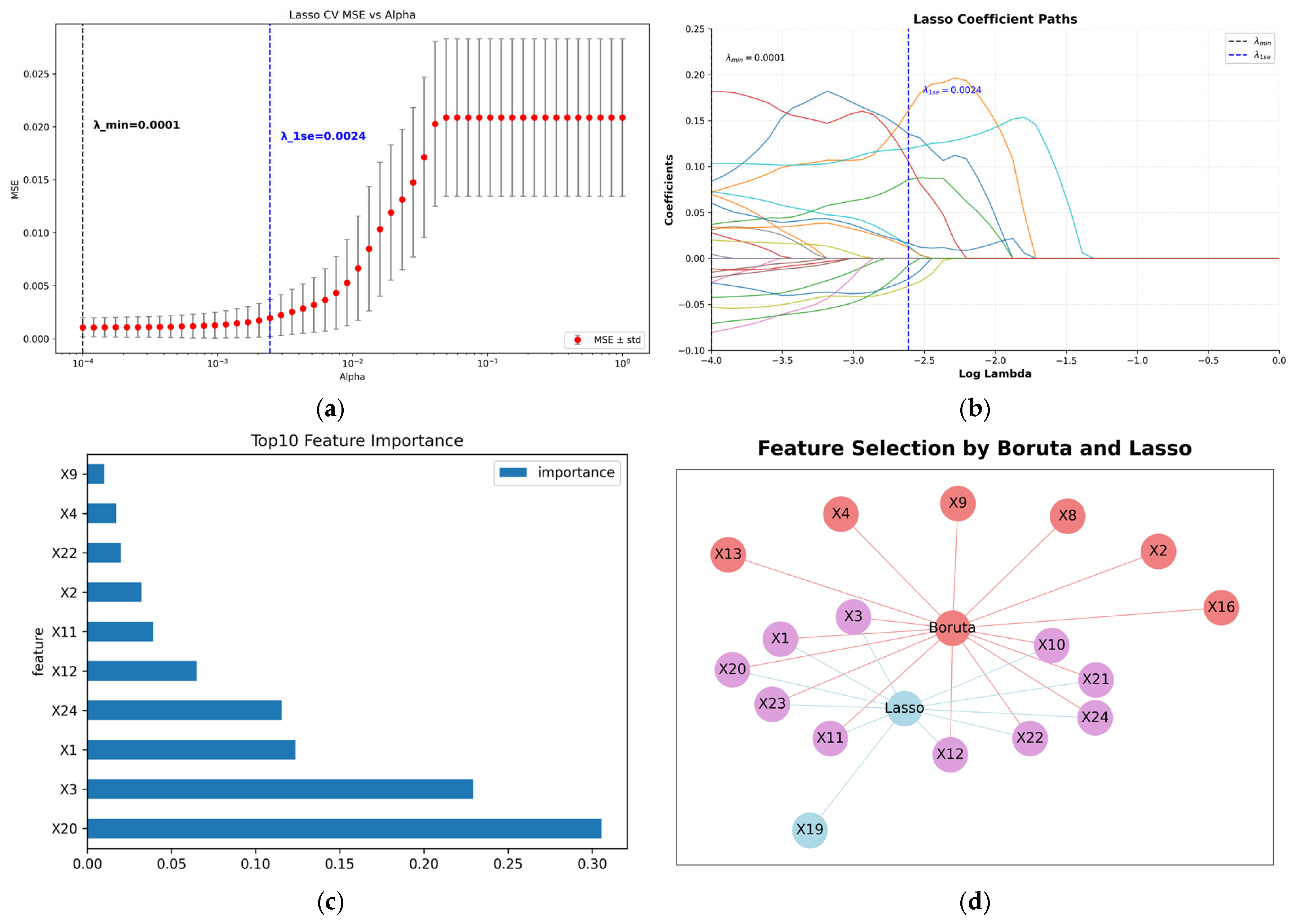
• Optimal regularization parameter tuning: The regularization parameter was optimized using LassoCV combined with RepeatedKFold (five-fold cross-validation, with three repetitions), setting alphas = np.logspace(−4, 0, 50) to construct a logarithmically spaced grid for a global search of regularization intensity. Using the cross-validated mean squared error (MSE) as the evaluation metric, the parameter corresponding to the minimum error was found to be ${\lambda }_{min}$ = 0.0001. Meanwhile, according to the 1-SE rule, a sparser and more generalizable regularization parameter of ${\lambda }_{1se}$ = 0.0024 was selected. Considering the model’s robustness and feature reduction requirements in the context of ship equipment price prediction, the final optimal regularization parameter ${\lambda }_{1se}$ was chosen to achieve greater feature sparsity and multicollinearity suppression while ensuring that predictive accuracy meets the requirements.
• Sparse selection results: Based on the ${\lambda }_{1se}$ training set, a Lasso model was constructed to remove redundant features whose coefficients were shrunk to 0, ultimately retaining 11 non-zero coefficient features, including X1, X3, X10, X11, X12, X19, X20, X21, X22, X23, and X24, achieving feature dimensionality reduction and multicollinearity suppression.

4.2.3. Intersection of Two-Stage Features and Construction of Final Feature Set

The intersection of the Boruta preliminary feature set and the Lasso (1 SE rule) refined feature set was taken to obtain doubly validated core significant features, ultimately forming a set of 10 optimal features: X1, X3, X10, X11, X12, X20, X21, X22, X23, and X24. This final feature set simultaneously meets the dual screening criteria of feature statistical importance according to the Boruta algorithm and sparsity according to the Lasso 1-SE rule. It retains key features with statistical explanatory power and contribution to the ordering price of naval equipment while maximally eliminating redundant features and alleviating multicollinearity interference, ultimately constructing an optimal feature subset that is dimensionally reduced, physically meaningful, and robust, providing high-quality input for subsequent predictive model training.

4.2.4. Visualization Analysis of Feature Selection Results

To visually present the two-stage feature selection process and results, this study plotted multidimensional visual charts (Figure 3). The core interpretations of each subfigure are as follows:

Figure 3a shows the variation curve of the Lasso cross-validation mean squared error (MSE), illustrating the trend of model MSE changes corresponding to different regularization parameters $\lambda$, which helps in selecting the optimal parameter. In the figure, the red dotted line represents the cross-validated average MSE for different $\lambda$ values, while the gray vertical lines indicate the standard deviation of the errors. Two vertical dashed lines mark ${\lambda }_{min}$ = 0.0001, corresponding to the minimum MSE, and ${\lambda }_{1se}$ = 0.0024, corresponding to a sparser solution that satisfies the 1 SE rule and has better generalization. It can be seen that as $\lambda$ increases, the MSE reaches a global minimum at ${\lambda }_{min}$, then the error increases monotonically and fluctuations become more significant. The error corresponding to ${\lambda }_{1se}$ is still within an acceptable range while achieving stronger feature sparsity, consistent with the objective of this study to “improve model robustness while ensuring prediction accuracy.”

Figure 3b is the coefficient path plot of the Lasso regression, showing the shrinkage process of each feature’s regression coefficient as the regularization parameter $\lambda$ increases. Each curve in the figure corresponds to the coefficient change trend of a feature. As the parameter $\lambda$ increases, the sparsity constraint of Lasso strengthens, and the coefficients of redundant features are gradually compressed to 0, intuitively reflecting its feature selection mechanism. The horizontal axis is on a logarithmic scale $lo{g}_{10}(\lambda )$, and the two vertical dashed lines in the figure indicate the positions of ${\lambda }_{min}$ (black dashed line, corresponding to $lo{g}_{10}(\lambda )$ ≈ −4) and ${\lambda }_{1se}$ (blue dashed line, corresponding to $lo{g}_{10}(\lambda )$ ≈ −2.6), respectively. It can be seen that at ${\lambda }_{min}$, the model’s regularization strength is low, and most feature coefficients are still non-zero; whereas at ${\lambda }_{1se}$, the coefficients of many redundant features have been compressed to 0, retaining only a few key features and achieving effective dimensionality reduction and multicollinearity suppression.

Figure 3c presents the top ten feature importance rankings obtained based on the random forest, quantifying the contribution of each feature to the prediction of ship equipment prices. The length of the bars represents the feature importance scores, with features X1, X3, X20, X24, and others scoring significantly higher than the rest, indicating that the above metrics have the most prominent impact on equipment prices. This is consistent with engineering practice, in which key factors such as displacement and core shipborne systems play a dominant role in determining costs, and it also highly overlaps with the core features selected through the two-stage screening.

Figure 3d presents the intersection network diagram of the Boruta–Lasso two-stage feature selection, which intuitively shows the overlap and differences between the results of the two methods. In the figure, purple nodes represent the core features confirmed by both methods (i.e., the 10 features used for the final modeling), red nodes are features retained only by the Boruta algorithm, and light blue nodes are nodes related only to the Lasso selection process. The relationships among nodes and edges clearly distinguish single-stage selected features from those verified by dual validation, fully reflecting the advantages of the two-stage selection strategy in terms of complementarity and robustness. It not only retains important features identified by the random forest but also further eliminates multicollinearity and noise interference through Lasso, resulting in intersection features that meet both importance and sparsity criteria.

4.3. Nonlinear Association Between Core Features and Target Prices of Ship Equipment Orders and Statistical Response Analysis

Based on the results of the two-stage Boruta–Lasso feature selection, this study ultimately identified 10 core features that affect the target price of ship equipment orders, namely X1, X3, X10, X11, X12, X20, X21, X22, X23 and X24. These indicators cover key dimensions such as the main scale of the ship, sustained endurance capability, weapon configuration, electronic detection equipment, and overall combat capability. Different features, through differentiated paths such as hull construction costs, procurement of onboard equipment, multi-system integration matching, and investment in supporting facilities, form a hierarchical statistical association effect with the target price of ship equipment orders. By combining the feature importance ranking results with ship engineering mechanisms, a unified analysis of the price effect mechanisms of the core features is conducted.

From the perspective of the main dimensional scale, X1 (full-load displacement) and X3 (ship beam) are fundamental indicators that determine ship size and construction cost, showing a strong statistical positive correlation with price. The larger the full-load displacement, the higher the costs of hull materials, compartment layout, piping installation, and overall processing, while also requiring a larger power system and supporting outfitting facilities, forming a positive fundamental driver for cost. Ship beam is directly related to ship stability design and deck space layout and also shows a significant statistical positive correlation with price. An increase in beam will raise the design standards for transverse hull strength and steel consumption, while providing more space for onboard weapons and electronic equipment, indirectly driving up equipment integration and construction costs. Combined with feature importance results, it can be seen that X1 and X3 rank among the top in core feature contributions and are the most critical fundamental size factors affecting the ship ordering price.

The higher the self-sustaining index, the more complex the ship supporting system, which is statistically positively correlated with price. A higher the -sustaining index requires larger reserve capacity for fuel, fresh water and living materials, resulting in more complex internal structure division and hull volume design. At the same time, it is necessary to support complete ventilation, water supply, energy storage and life support systems, which not only increase the construction cost of the hull structure but also increase the procurement investment in supporting outfitting and support equipment, which has a stable positive impact on the overall order price of the ship.

The dimensions of weapons and equipment, electronic detection, and comprehensive combat power include a total of seven core characteristics:X11, X12, X20, X21, X22, X23, and X24, which are the leading factors most strongly statistically correlated with the high-price segment. Among them, the number of Vertical Launch Missile System Units X11 and the number of Vertical Launch Missile Systems X12 directly determine the ship’s air-to-sea strike capability. An increase in the number of missile vertical launch system configurations will bring about the synchronous upgrade of launchers, fire control units, power supply cooling and structural support systems, significantly increasing the cost of equipment procurement and system integration, which are strongly statistically positively correlated with price. The interference rocket launcher X19, phased array radar X20, other radars X21, and sonar system X22 correspond to the core functions of ship electronic countermeasures, long-range detection and early warning, and anti-submarine warning, respectively. Comprehensive combat capability indicators, such as the number of ship cannons X23 and equipment combat effectiveness X24, are highly statistically positively correlated with price. The higher the level of comprehensive combat power, the more complete the overall supporting system and the more stringent the technical standards, simultaneously driving up the costs of construction, procurement, integration and testing throughout the whole process.

In summary, the 10 core features identified in this study can be divided into three main categories: main scale and tonnage, self-sustaining support capability, and weapon electronics and comprehensive combat capability. These features do not act independently; instead, they interact through multiple aspects, such as hull structure design, onboard system integration, electromagnetic compatibility adaptation, and combat system integration, forming coupled synergistic effects and exhibiting a stepwise statistical correlation with the target procurement cost of the ship. At the same time, the feature importance rankings corroborate the mechanism analysis, indicating that the two-stage feature selection results possess good engineering interpretability and practical rationality.

4.4. Model Performance

Select 10 key features after feature screening as input variables, and the target price for ship equipment orders as the output variable. Split the dataset into a training set and a test set at a ratio of 7:3, and select a validation set from the training set at a ratio of 12.5%. To control model complexity and reduce the risk of overfitting with small samples, use five-fold repeated cross-validation (three repetitions) combined with grid search (GridSearchCV) to optimize the hyperparameters of the CatBoost model. The optimized parameters include learning rate, number of iterations, and tree depth, with the parameter search ranges and optimal values shown in

Table 2. CatBoost parameter optimization table. Note: All model input features are normalized to the [0, 1] range using min–max scaling.

Algorithm	Parameter	Parameter Grid	Optimal Value
CatBoost	learning_rate	[0.005, 0.01, 0.02, 0.05, 0.1]	0.1
	iterations	[100, 200, 500, 1000]	500
	depth	[1, 2, 9, 10]	2

.

It should be noted here that the tree depth of the CatBoost model directly determines the highest-order feature interactions it can capture. A decision tree with depth d can model feature interactions up to order d. In this study, the optimal tree depth is two, which can fully capture all second-order feature interactions, completely covering the most critical binary feature synergy effects in ship equipment design (such as the combined impact of the number of vertical launch units and phased array radar configurations). Grid search results show that increasing the tree depth (e.g., depth = 10) does not improve cross-validation performance and instead introduces unnecessary complexity. At the same time, the ensemble properties of 500 shallow trees can still fit complex nonlinear relationships; therefore, there is no risk of underfitting.

The optimal parameters were used to build the model to obtain the final predictive model, and its performance on the test set is shown in

Table 3. Model performance indicators. Note: RMSE and MAE are both calculated based on the normalized target price, with prices normalized to the [0, 1] range.

Evaluation	Optimal Single Result	Results of 10 Repeated Validations (Mean ± Standard Deviation)
R2	0.8949	0.8828 ± 0.0000
RMSE	0.0554	0.0586 ± 0.0000
MAE	0.0476	0.0529 ± 0.0000

. All evaluation metrics are calculated based on normalized prices.

The optimal single-run results of the model are: coefficient of determination (R²) of 0.8949, root mean square error (RMSE) of 0.0554, and mean absolute error (MAE) of 0.0476, indicating that the model has strong explanatory and fitting capabilities for the data. To further verify the robustness and repeatability of the model, this study conducted 10 independent repeated trainings by fixing the training/testing set split and only changing the model’s random seed. The results show that the average performance of the model on the test set is R² = 0.8828 ± 0.0000, RMSE = 0.0586 ± 0.0000, and MAE = 0.0529 ± 0.0000. Since the prices have been normalized to the [0, 1] range, the fluctuations across the 10 experiments were extremely small, and rounding in the original text showed values of 0.0000, while the actual standard deviations were in the range of 0.0002–0.0003. The optimal single-run results are highly consistent with the average results from multiple repetitions, indicating that the model not only has high-precision predictive capability but also maintains stable performance with minimal fluctuation under different initialization conditions, without overfitting or random dependency. To avoid overestimating performance due to interpolated samples, an independent test was conducted on 33 original real samples, resulting in R² = 0.8166, RMSE = 0.0733, and MAE = 0.0576. The performance remains robust, verifying the model’s generalization ability and engineering applicability across different data subsets.

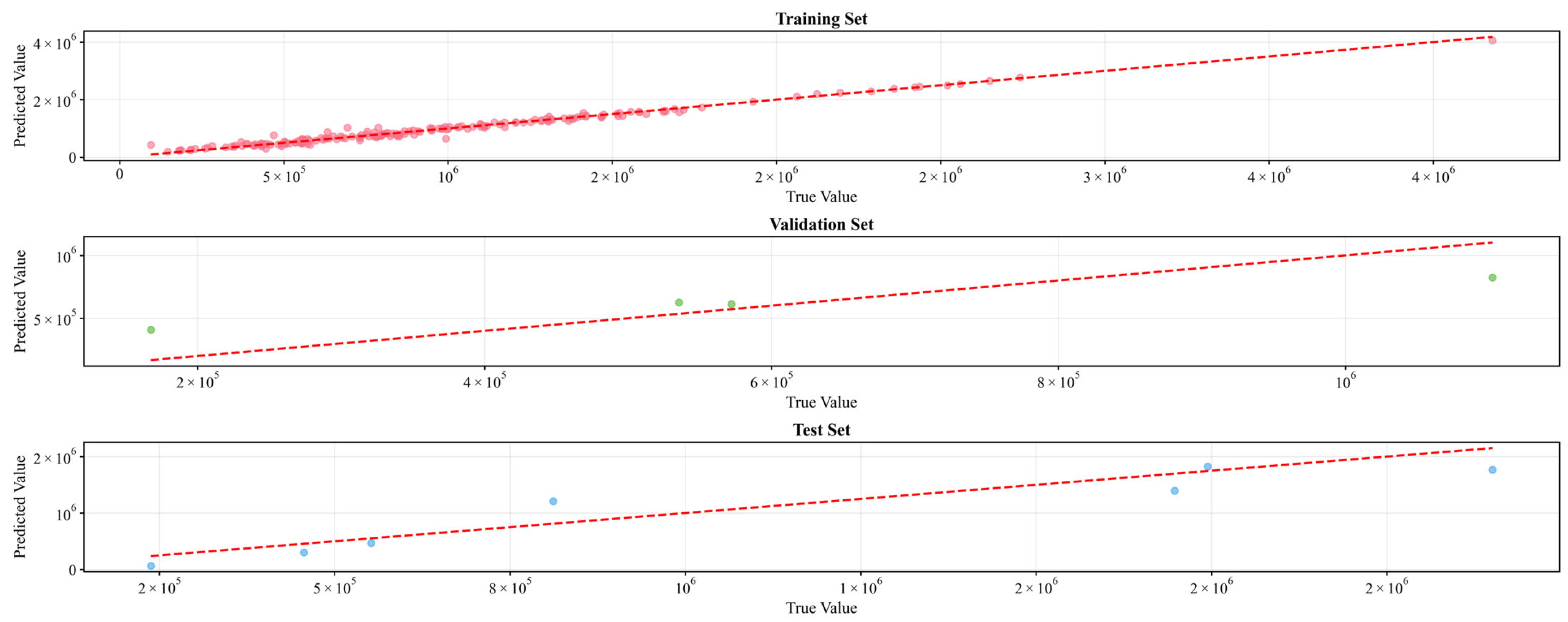
The model’s predictive performance on the training set, validation set, and test set is shown in Figure 4. As seen in the figure, the sample points of all three datasets are closely distributed around the fitting line, with no obvious systematic bias, indicating that the model demonstrates good predictive consistency during training, validation, and testing. The predicted results of the training set, validation set, and test set all exhibit linear relationship that highly matches the true values, and the performance differences among the subsets are small, suggesting that the model has good fitting ability, generalization capability, and stability in predicting target prices for ship equipment orders, with no obvious overfitting or underfitting phenomena.

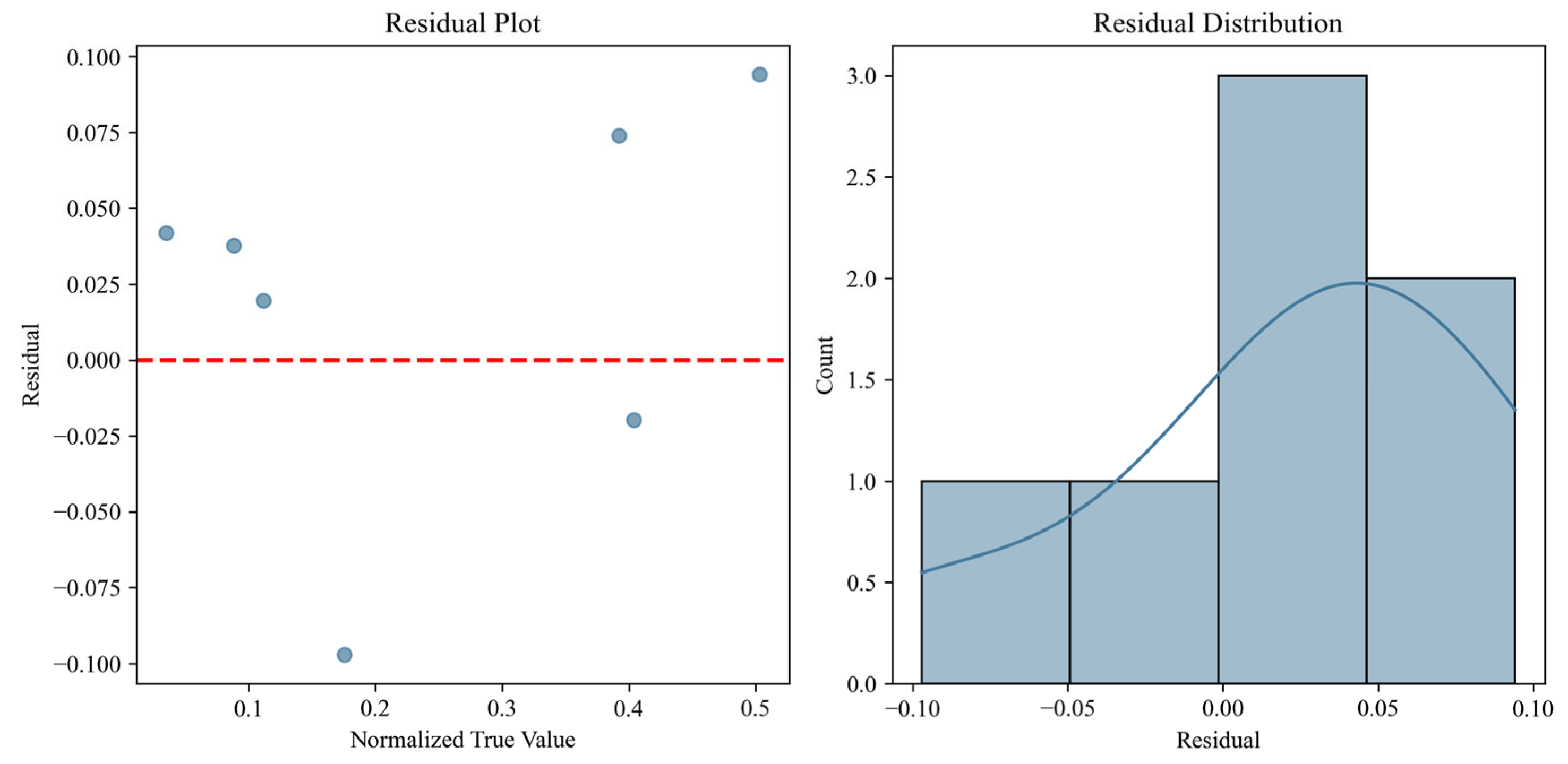
The results of the normalized residual analysis are shown in Figure 5. In the residual scatter plot on the left, all normalized residuals are evenly distributed around the zero baseline, with no obvious trend shifts or funnel-shaped divergence features. The residual distribution histogram on the right shows that the residuals approximately follow a normal distribution centered at 0, with a symmetric and concentrated distribution. The normalized residual statistics indicate that the mean of the normalized residuals in the test set is only 0.0089, which is close to 0 overall, with no systematic positive or negative bias. The standard deviation of the normalized residuals is 0.0639, indicating small fluctuations in prediction errors. Dividing the high- and low-price ranges based on the median of the normalized true values, the standard deviation of normalized residuals in the low-price range is 0.0203, whereas that in the high-price range is 0.0313. The residual dispersion in the high-price range is slightly increased, but the difference between the ranges is limited. Further, the Levene’s test for homogeneity of variance was used to determine heteroscedasticity. The Levene statistic is 0.0010, with a corresponding p-value of 0.9757, which is significantly greater than the 0.05 significance level. This indicates that the variances of normalized residuals across different price ranges are homogeneous, the model does not present significant heteroscedasticity, and the prediction errors are stable and reliable across the entire sample range.

4.5. Model Explanation

4.5.1. Individual Explanation

Figure 6 shows the SHAP explanation plot for a randomly selected sample, intuitively presenting the direction and strength of each feature’s contribution to the prediction result for this sample. In the figure, the horizontal axis represents the model’s predicted value (after normalization), and the central base value is the average predicted value across all samples. The final predicted value for this individual sample is 0.41, which is higher than the baseline value. The contribution of features to the predicted value is indicated by arrows: arrows extending to the right (red) indicate that the feature increases the predicted value, representing a positive contribution; arrows extending to the left (blue) indicate a reduction in the predicted value, representing a negative contribution.; and the length of the arrow reflects the strength of the contribution. From Figure 6, it can be seen that the predicted value of this sample is higher than the baseline value, mainly driven by positively contributing features, with no negatively contributing features. The features with the most significant effects on increasing the predicted value are X22, X24, X12, X20, X1, X3, X11, and X21, collectively raising the predicted value to 0.41.

4.5.2. Comprehensive Explanation

SHAP heatmaps can only reveal the impact of features on the target price of ship equipment orders for specific samples, while SHAP value visualizations based on the entire sample (Figure 7 and Figure 8) provide overall distribution and stability information for the contributions of all input features to price.

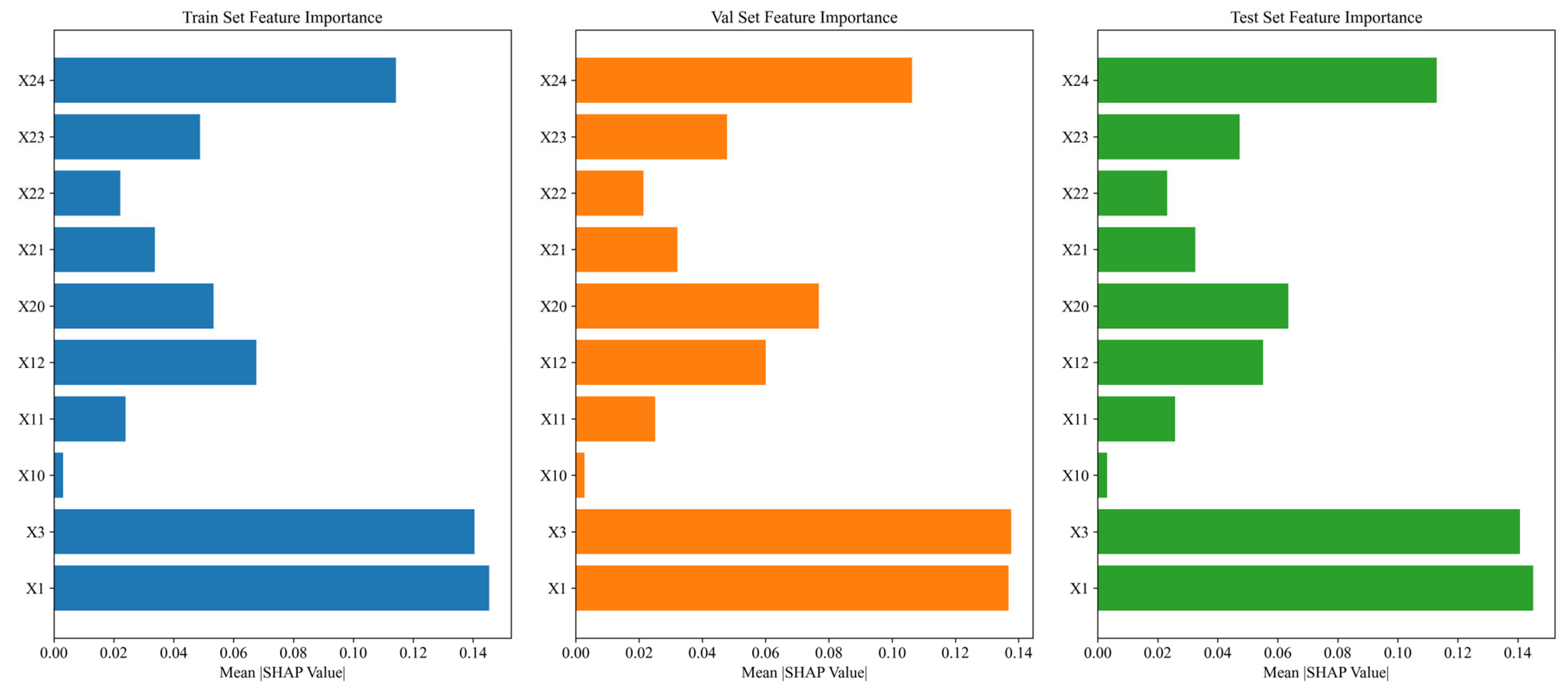
Figure 7 is a feature importance ranking chart based on the mean absolute SHAP values, showing the statistical contribution strength of each feature to the predicted target price of ship equipment across the training, validation, and test sets. Feature importance is positively correlated with its mean absolute SHAP value; a larger value indicates that the feature has a more significant statistical impact on predicting the target price of ship equipment. As shown in Figure 7, across the three data subsets—training, validation, and test sets—X1 (full-load displacement of the ship) has the highest mean absolute SHAP value and is the most important influencing factor in the model. This is followed by X3 (ship width), X24 (equipment combat power), X20 (number of phased array radars), X12 (number of Vertical Launch Missile Systems), and X23 (number of naval guns), whose importance rankings show high consistency across the training, validation, and test sets. Among them, X1, X3, X24, X20, and X12 consistently rank higher than other features across different data subsets, indicating that these factors contribute robustly to model predictions and align with existing research conclusions regarding the impact of main ship dimensions and key equipment configurations on costs [56,57]. To further verify the stability of the core feature explanations, we calculated the variance of SHAP values for X20 across each dataset, with variances of 0.002001, 0.000003, and 0.002745 for the training, validation, and test sets, respectively, and a test-to-training variance ratio of 1.37. This ratio is less than 1.5 and falls within a reasonable fluctuation range, indicating that the model’s explanatory power for X20 did not shift in the test set and showed no signs of overfitting or explanation instability. The importance ranking of this feature consistently remains among the top across different datasets, and the slight fluctuations in mean SHAP values are caused only by differences in sample distributions among the subsets, demonstrating overall good explanation robustness.

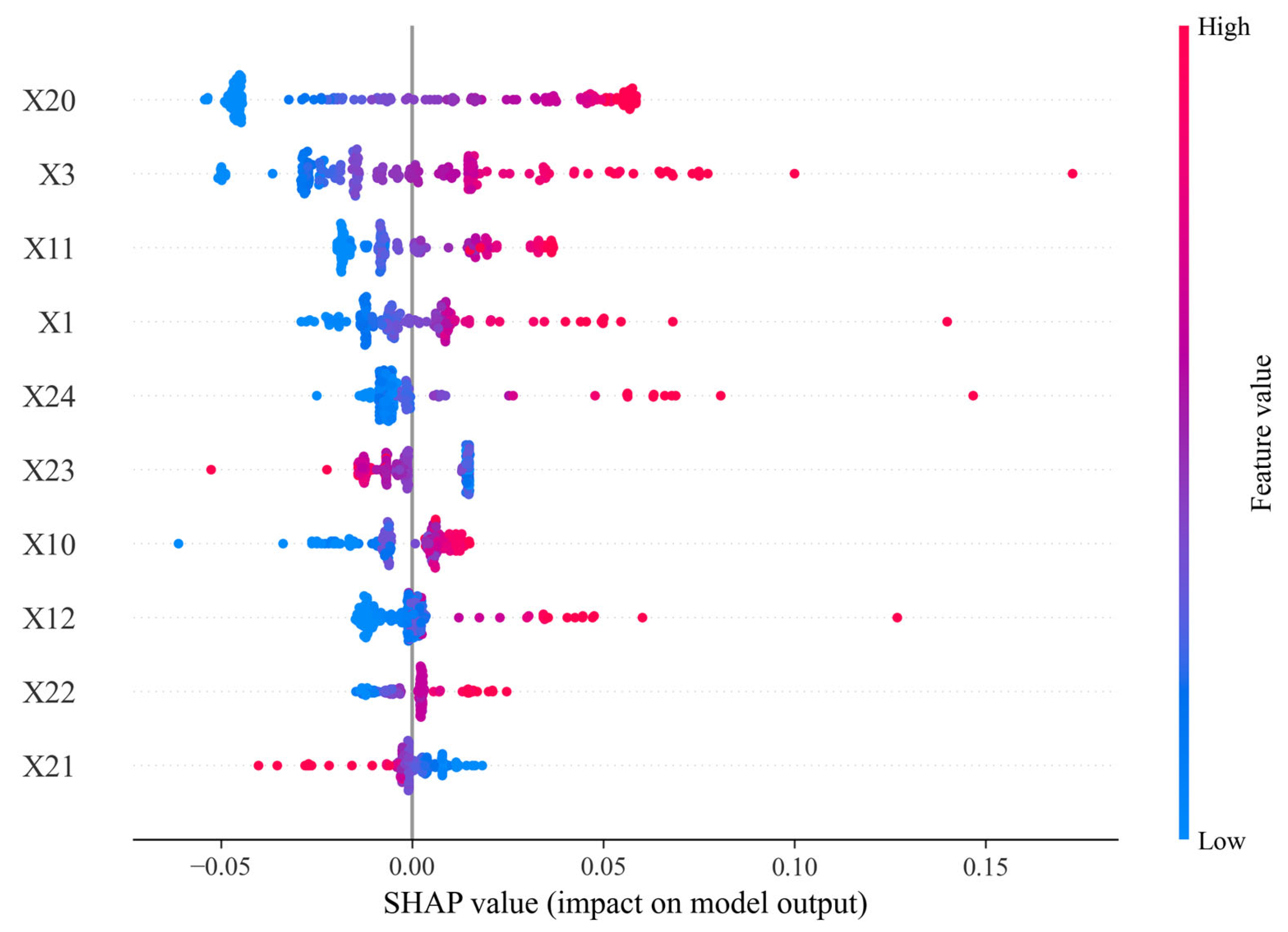
Figure 8 is a summary chart of SHAP global explanations for features, visually presenting the statistical contribution strength and direction of influence of each feature on the target price prediction of ship equipment orders, as well as the relationship between feature values and SHAP values. In the figure, features are sorted from top to bottom based on their global importance. The color of the dots represents the magnitude of the feature values (red for high feature values and blue for low feature values), and the horizontal axis represents SHAP values: positive values indicate a positive contribution to the prediction, while negative values indicate a negative contribution. From the figure, it is clear that features such as X20, X3, X11, X1, X24, and X12 are at the top, with a wider distribution range of SHAP values and a more significant impact on the model’s prediction results, making them the core driving factors determining the target price of ship equipment orders. For key features like X20, X3, X1, X24, and X12, high feature values (red dots) are highly concentrated in the positive SHAP value region, indicating that when these features take high values, they significantly increase the model’s predicted value for the target price of ship equipment orders, showing a stable positive correlation. In contrast, low feature values (blue dots) are mostly distributed in the negative SHAP value region, corresponding to lower prediction contributions, which fully aligns with the theoretical logic in the ship cost domain: the larger and higher-grade the main scale of the ship (X1, X3) and the core equipment configurations (X12, X24, X20), the higher the corresponding equipment order price level.

4.5.3. Main Feature Dependency

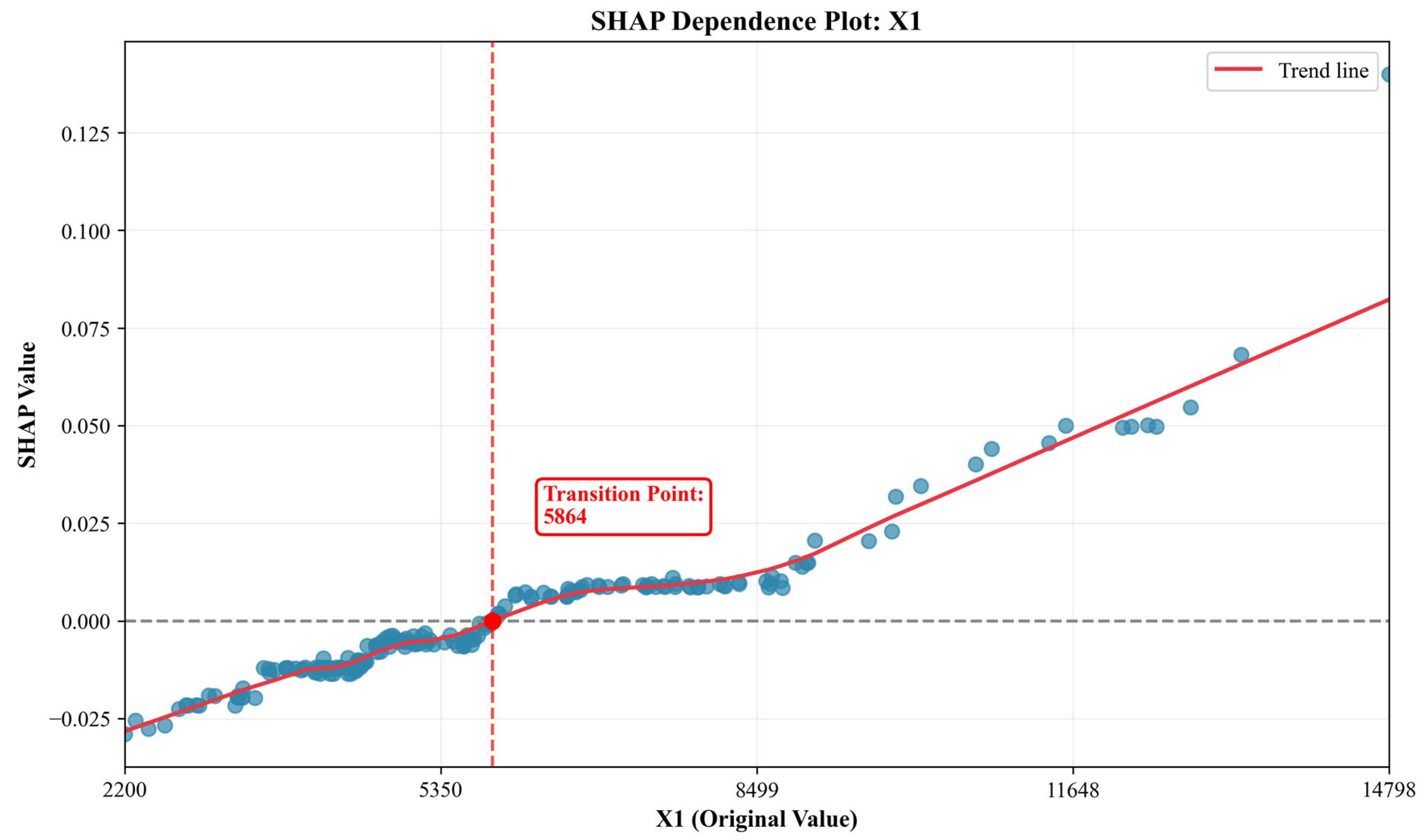
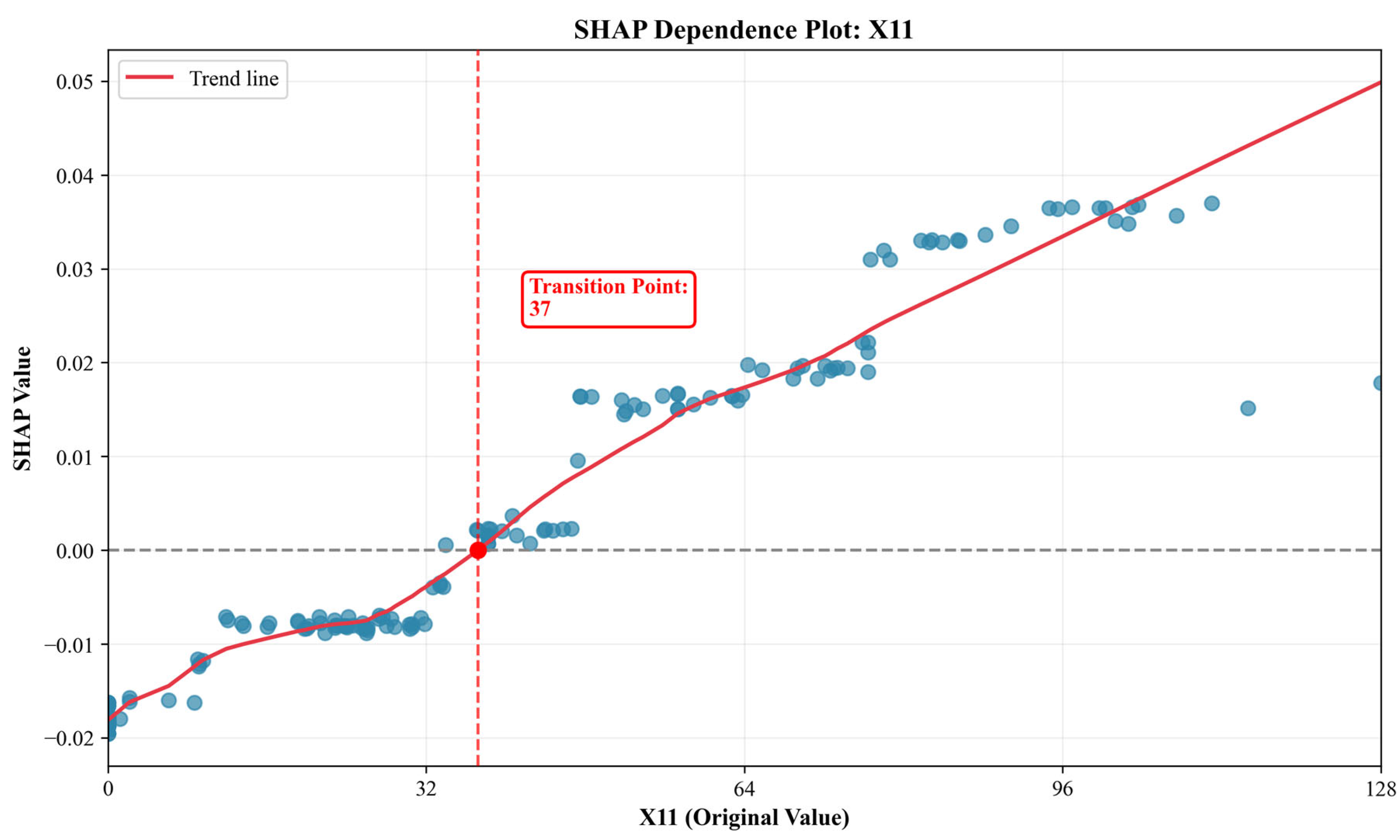
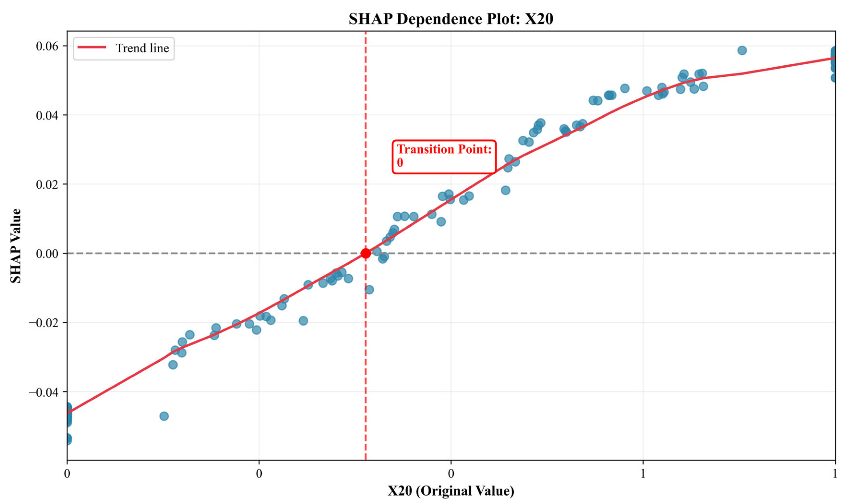
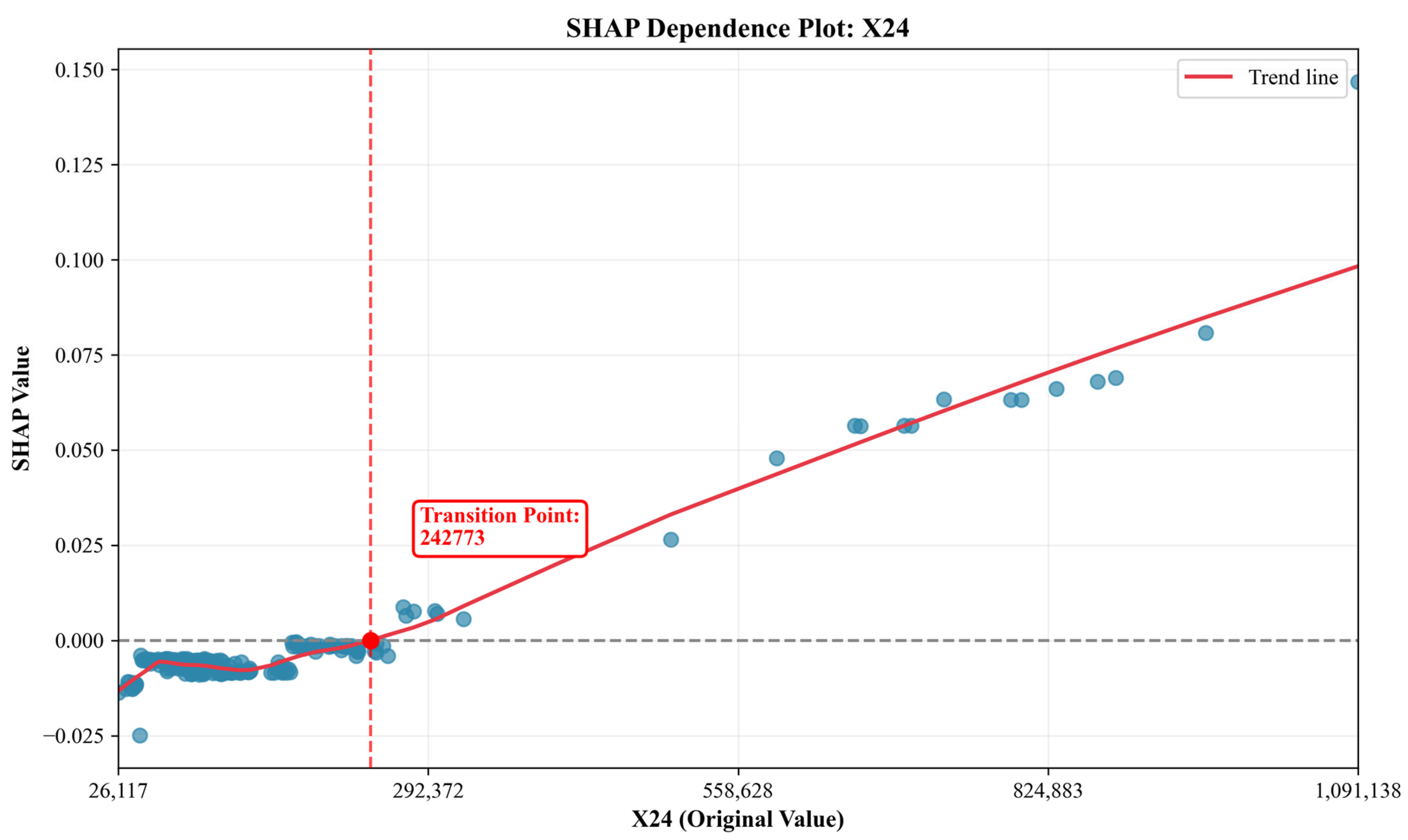
To further reveal the statistical response patterns of target prices for ship equipment procurement, this section uses the SHAP (SHapley Additive exPlanations) method to perform interpretability analysis on the CatBoost model, focusing on the nonlinear statistical relationships between core features such as full-load displacement (X1), number of Vertical Launch Missile System Units (X11), number of phased array radars (X20), combat capability of equipment (X24), and price. Figure 9, Figure 10, Figure 11 and Figure 12 show the SHAP dependence plots for each key feature, where blue scatter points represent SHAP values of individual samples, the red curve is the nonlinear trend line based on LOWESS (locally weighted scatter plot smoothing), the horizontal dashed line is the baseline where the SHAP value equals zero, and the marked points represent the intersection of the trend line with the zero baseline (i.e., statistical response transition point where the feature’s effect on price shifts from negative to positive). LOWESS uses the parameters frac = 0.3 (meaning that the local fitting window covers 30% of the total samples) and it = 3 (three iterations). This setting ensures a smooth trend line while effectively preserving the nonlinear variations and key statistical response transition points in the data, avoiding excessive smoothing that might obscure the true interactions between features and price.

• Statistical response of full-load displacement (X1)

As shown in Figure 9, X1, as the core indicator of ship size and construction scale, exhibits a significant nonlinear increase in SHAP values with increasing displacement, together with a clearly observable statistical response transition point. This study uses LOWESS fitting and the SHAP = 0 intersection method to determine the transition point and obtains the 95% confidence interval through 100 bootstrap resamplings. The results show that the statistical response transition point of full-load displacement is 5864 tons (95% CI: 5571–6157 tons). When the full-load displacement is below the transition point (5864 tons), the SHAP value is negative, indicating that increases in displacement have a weak marginal effect on price or even a cost-dilution effect influenced by factors such as construction processes and material utilization. When the displacement exceeds this transition point, the SHAP value turns from negative to positive and continues to rise, showing a typical increasing marginal statistical response characteristic. This result indicates that increasing ship size not only directly raises basic costs such as hull structure and propulsion systems, but also forms a nonlinear positive feedback mechanism between “size and cost” due to accommodate larger-scale onboard systems and enhanced redundancy design standards, which highly aligns with the engineering practice rule that the construction costs of large ships rise rapidly with tonnage. The LOWESS curve clearly captures this transition point, validating the model’s precise depiction of the nonlinear relationship between tonnage and cost.

2.

Statistical Response of the Number of Vertical Launch Missile System Units (X11)

As shown in Figure 10, X11 is a key indicator for measuring the ship’s firepower delivery capability. Its SHAP dependence curve exhibits a segmented nonlinear feature of “negative first, then positive,” together with a clear statistical response transition point (37 units). Based on LOWESS fitting and the SHAP = 0intersection method, and after 100 bootstrap resampling iterations, the transition point was determined to be 37 units (95% CI: 35–39 units). When the number of vertical launch system (VLS) cells is below the transition point (37 units), the SHAP value is negative, indicating that configuring a small number of VLS cells has a limited marginal contribution to the price. In fact, due to the cost distribution effect of a modular system, the cost impact per unit is diluted. When the number of units exceeds the transition point, the SHAP value turns positive and continues to rise, with the curve slope gradually increasing as the number of units grows. The core reason for this phenomenon is that the cost of the vertical launch system includes both fixed costs for platform adaptation, fire control system integration, ammunition compatibility design, and unit manufacturing costs. Once the number of units exceeds the critical scale, the fixed costs are sufficiently distributed, and the marginal cost proportion of additional units significantly increases. Meanwhile, upgrading supporting facilities such as power supply and cooling systems to accommodate more units further drives up the price, showing a clear pattern of increasing marginal costs. The LOWESS smoothed curve accurately reflects the nonlinear jump process of the impact of VLS cell number on price.

3.

Statistical Response of Phased Array Radar Quantity (X20)

As shown in Figure 11, X20 is the core equipment for shipborne detection and command capabilities. Its SHAP value shows a clear nonlinear transition from negative to positive as the number of radars increases, with the statistical response transition point at 0 units (representing no phased array radar configured). The transition point was determined using LOWESS fitting and the SHAP = 0 intersection method, while the uncertainty interval was obtained through bootstrap sampling. The results show that the statistical response transition point is 0 units (95% CI: 0–1 units), meaning that when no phased array radar is configured, the SHAP value is negative, whereas with one or more units configured, the SHAP value quickly turns positive and rises exponentially, reflecting the cost-leap effect of high-end electronic equipment from absence to presence. When the number of phased array radars is 0 (not configured), the SHAP value is negative, indicating that without this configuration, there is no positive impact on the ship’s price, and due to fixed inputs such as reserved interfaces on the basic platform and generalized design, a cost-dilution effect is observed. When the number is greater than 0 (one or more units configured), the SHAP value shifts from negative to positive and rises rapidly, with the curve showing a significant exponential growth trend. This pattern accurately reflects the cost characteristics of phased array radars: when not configured, there is no incremental cost for core electronic systems; once actually configured, it is necessary to simultaneously address challenging technical issues such as electromagnetic compatibility, multi-target cooperative detection, and data fusion, while upgrading supporting high-value systems for power supply, cooling, and command control. The cost increases nonlinearly and rapidly with the number of equipment, fully reflecting the technological premium and marginal cost escalation of high-end shipborne electronic systems from absence to presence. The LOWESS smoothed curve clearly demonstrates this ‘from nothing to something’ cost-leap process.

4.

Statistical Response of Equipment Combat Power (X24)

As shown in Figure 12, X24, as a quantitative indicator of the integrated combat effectiveness of a ship, exhibits a ‘negative-to-positive’ nonlinear growth trend in its SHAP dependence curve, with the statistical inflection point feature being the most significant. The transition point was determined based on LOWESS and the SHAP = 0 intersection method, and the confidence interval was calculated using 100 bootstrap resamples, resulting in a transition point of 242,773 combat power (95% CI: 230,634–254,912 combat power). When the equipment combat power is below the transition point (242,773 combat power), the SHAP value is negative, indicating that lower equipment combat power corresponds to a lower ship configuration level with limited incremental costs, which may even be diluted due to the scale effect of the basic platform. When the equipment combat power exceeds the transition point, the SHAP value turns from negative to positive and rises sharply, showing a typical characteristic of an increasing marginal statistical response. This result indicates that the improvement in equipment combat power is not a linear cost increase; rather, there exists a clear ‘effectiveness-cost’ critical point. Below the critical point, enhancing equipment combat power mainly relies on optimizing the configuration of basic weapons and electronic systems, resulting in relatively lower cost increments. After exceeding the critical point, the introduction of high-end weapon systems, advanced electronic equipment, stealth design, and other complex technologies is required, along with upgrades to platform adaptability, leading to nonlinear rapid cost growth as equipment combat power increases, reflecting the technological premium and marginal cost escalation of high-performance ships. The LOWESS smoothed curve accurately identified this key inflection point, validating the model’s ability to characterize the nonlinear relationship between effectiveness and cost.

4.6. Model Performance Comparison

4.6.1. Overall Model Performance Comparison

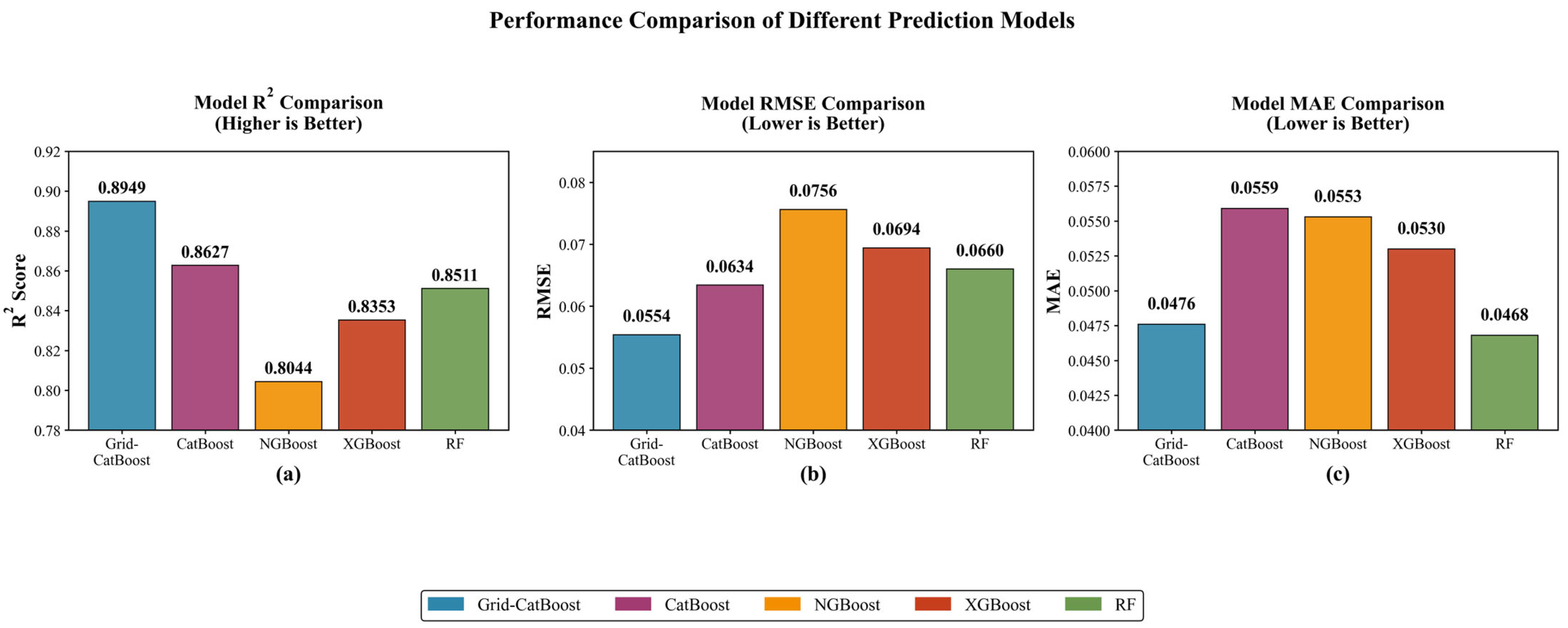
To further validate the predictive performance of the proposed model, this paper compares the Grid-CatBoost model with CatBoost, NGBoost, XGBoost, and random forest (RF) models. The comparison results are shown in Figure 13, while the performance metrics of each model are detailed in

Table 4. Comparison of model performance. Note: RMSE and MAE were both calculated based on the normalized target price, with prices normalized to the [0, 1] range. The p-value is the result of the paired t-test between the Grid-CatBoost model and the corresponding model (based on the mean squared error of 10 repeated experiments), with p < 0.05 indicating that the difference is statistically significant.

Model	Optimal Single Result			Results of 10 Repeated Validations (Mean ± Standard Deviation)			p-Value	Significance
	R2	RMSE	MAE	R2	RMSE	MAE
Grid-CatBoost	0.8949	0.0554	0.0476	0.8828 ± 0.0000	0.0586 ± 0.0000	0.0529 ± 0.0000	——	——
CatBoost	0.8627	0.0634	0.0559	0.8459 ± 0.0000	0.0671 ± 0.0000	0.0617 ± 0.0000	0.021	p < 0.05
NGBoost	0.8044	0.0756	0.0553	0.8045 ± 0.0002	0.0756 ± 0.0000	0.0553 ± 0.0003	0.0004	p < 0.001
XGBoost	0.8353	0.0694	0.0530	0.8215 ± 0.0105	0.0722 ± 0.0022	0.0549 ± 0.0022	0.003	p < 0.01
RF	0.8511	0.0660	0.0468	0.8457 ± 0.0091	0.0671 ± 0.0020	0.0486 ± 0.0014	0.008	p < 0.01

. The best single-run results indicate that the Grid-CatBoost model achieved a coefficient of determination (R²) of 0.8949, a root mean square error (RMSE) of 0.0554, and a mean absolute error (MAE) of 0.0476, all of which outperform other comparison models. All error metrics are calculated based on the same normalized price scale, ensuring full consistency among the compared models. Compared with the second-best CatBoost model, its RMSE is reduced by approximately 12.62%, demonstrating higher predictive accuracy. To verify model stability, ten repeated experiments were conducted using a fixed training/testing split while only changing the model’s random seed to avoid bias introduced by data partitioning. The results show that the average performance of the Grid-CatBoost model is R² = 0.8828 ± 0.0000, RMSE = 0.0586 ± 0.0000, and MAE = 0.0529 ± 0.0000. Since the prices were normalized to the [0, 1] range, the fluctuations across the ten experiments were minimal, with the standard deviation displayed as 0.0000 when rounded to four decimal places; the actual fluctuations were on the order of 10⁻⁴, indicating highly stable model performance without random dependency. As shown in Table 4, the Grid-CatBoost model exhibits optimal performance both in the best single-run results and across the ten repeated experiments. Paired t-test results demonstrate that the performance differences between this model and CatBoost, NGBoost, XGBoost, and RF models are statistically significant (all p < 0.05), confirming its superiority and robustness in predicting target prices for naval equipment procurement tasks.

4.6.2. Ablation Study

To verify the effectiveness of the Boruta–Lasso combined feature selection strategy, this study designed an ablation control experiment consisting of four schemes: a full-feature baseline, single Boruta selection, single Lasso selection, and Boruta–Lasso two-step selection. These schemes were systematically compared to evaluate the impact of different feature selection methods on model predictive performance and multicollinearity mitigation. The experiment selected the coefficient of determination (R²), root mean square error (RMSE), mean absolute error (MAE), and variance inflation factor (VIF) as evaluation indicators, and the results are shown in

Table 5. Comparison of ablation studies. Note: RMSE and MAE were both calculated based on normalized target prices; features and prices were normalized using min–max scaling. VIF is the variance inflation factor, which is used to measure the degree of multicollinearity among features. A VIF > 10 indicates significant multicollinearity, which was significantly alleviated after feature selection.

Feature Selection	R2	RMSE	MAE	Number of Features	Average VIF	Highest VIF	p-Value	Significance
Boruta–Lasso	0.8949	0.0554	0.0476	10	8.68	32.03	——	——
Boruta	0.8333	0.0698	0.0520	16	11.05	69.21	0.0012	p < 0.01
Lasso	0.8744	0.0606	0.0481	11	8.27	33.45	0.0178	p < 0.05
Full features	0.8612	0.0637	0.0486	24	18.01	119.95	0.0068	p < 0.01

. From the VIF results, it can be seen that the full-feature set contains obvious multicollinearity (average VIF = 18.01). After selection by individual methods, multicollinearity is somewhat improved. After Boruta–Lasso two-stage selection, feature collinearity is significantly reduced and the feature set is more streamlined, indicating that this strategy can effectively reduce feature redundancy and multicollinearity while ensuring model accuracy, achieving the best overall performance.

As shown in Table 5, the overall performance of the four feature selection strategies is relatively close. The two-stage Boruta–Lasso method achieved the best values in R², RMSE, and MAE, slightly outperforming the single-selection methods and the full-feature scheme, indicating that this strategy has some effect in enhancing model accuracy and stability, although differences among the groups are not significant.

The single Boruta selection scheme performs relatively weakly, with an R² of only 0.8333, and RMSE and MAE of 0.0698 and 0.0520, respectively. This method completes only preliminary coarse feature screening; although it retains core relevant features, it does not achieve precise feature dimension reduction, and redundant features and noise interference still exist, limiting improvements in model predictive accuracy.

The single Lasso selection scheme shows some improvement over the full-feature baseline, with R² increasing to 0.8744 and RMSE and MAE decreasing to 0.0606 and 0.0481, respectively. This is attributed to the sparse regularization mechanism of the Lasso algorithm, which can effectively eliminate irrelevant noise features and redundant variables, achieve feature dimensionality reduction, and reduce prediction bias.

When using the two-step Boruta–Lasso linkage screening strategy, the model’s overall performance reaches the optimum: R² increases to 0.8949, RMSE decreases to 0.0554, and MAE decreases to 0.0476. All indicators are slightly better than those of the single-selection schemes and the full-feature baseline, with overall performance being relatively close.

In conclusion, reasonable feature selection can optimize the quality of model input features and improve predictive accuracy and stability. The two-step Boruta–Lasso linkage strategy combines high efficiency with strong robustness and offers high screening accuracy. It fits the feature selection needs and predictive modeling tasks of this study and can be considered the preferred scheme for feature selection in price prediction models of similar equipment.

4.7. Policy Research

Based on the identification of core correlation characteristics and model interpretable analysis of the target price of ship equipment orders, combined with the theory of whole-lifecycle economic assessment for ships [50,51,52,53,55], the following engineering management suggestions are put forward from five dimensions: pricing standardization, precise cost control, decision-making digitalization, efficiency–cost balance, and dynamic prediction support: pricing standardization, cost precise control, decision-making digitalization, efficiency–cost balance, and dynamic prediction support.

• Construct a hierarchical classification pricing standard based on core statistical association characteristics. Based on key related characteristics such as full-load displacement, number of missile vertical launch units, phased array radar configuration, and comprehensive combat effectiveness, a benchmark price system for ship equipment ordering by tonnage, configuration, and combat power level should be established to replace the traditional subjective estimation model and improve the standardization, consistency and traceability of pricing.
• Implement precise control across the whole chain of cost-related elements. Focus on high-cost modules such as hull structures, power systems, shipboard electronic equipment and weapon systems, and reduce the unit price of core equipment through large-scale procurement, modular design, and localized substitution. At the same time, implement on-demand configuration for high-value equipment such as vertical launch systems and phased array radars to avoid functional redundancy and inflated costs.
• Establish a data-driven closed loop for price demonstration and review. Build a standardized database of technical parameters, configuration schemes and purchase prices of ship equipment, and embed the Boruta–Lasso-CatBoost-SHAP integrated model into the equipment pricing demonstration process to form a closed loop of “feature screening–high-precision prediction–explainable attribution–review decision-making”, improving the scientificity and transparency of pricing decisions.
• Optimize equipment efficiency–cost allocation based on nonlinear statistical transition points. Relying on the inflection point law of statistical response revealed by SHAP dependency (displacement, vertical unit, and transition points of combat effectiveness), the equipment configuration structure is optimized under the premise of meeting combat needs, the optimal cost-effective interval is identified, and the balanced matching between combat effectiveness and procurement cost is realized.
• Improve dynamic price correction and medium- and long-term forecasting mechanisms. Integrate external factors such as industrial producer price index, supply chain fluctuations, and technology iteration to construct a dynamic price adjustment model. The forecasting framework of this paper is used to predict the cost trend of the whole-lifecycle of ship equipment, which provides stable support for equipment development planning, budgeting and fund coordination.

4.8. Discussion of Research Limitations and Shortcomings

This study has achieved certain results in predicting target prices for ship equipment orders and analyzing their feature associations. However, due to limitations in data conditions, model assumptions, and research scope, there are still a number of limitations:

• Limited scale of original real samples is. In this study, there were only 33 original real samples. Although data augmentation through interpolation expanded the dataset to 198 samples for modeling, the interpolated samples are only a means of data augmentation and are not considered independent empirical samples. The limited amount of original data may still pose certain risks of fluctuation in the model’s generalization ability and the estimation of statistical response transition points.
• Price data come from public sources, and some data cannot be independently verified. Ship procurement prices involve defense secrets. This study used only public quotations and contract prices, without obtaining internal data such as actual shipyard costs, labor, and materials. As a result, some price information is difficult to cross-verify.
• Historical military procurement prices have potential biases. Military procurement is influenced by non-technical factors such as international politics, arms trade policies, batch sizes, and cooperation agreements. Historical prices may contain certain non-market biases that could affect the stability of statistical associations.
• Inflation and currency exchange introduce uncertainty. The research involves multiple currencies and cross-year prices. Although exchange rate conversion and inflation adjustment were applied, statistical errors in equipment price indices and military inflation coefficients across different countries may still bring uncertainty into the price benchmarks.
• Multicollinearity in ship design variables. Equipment characteristics such as displacement, main dimensions, propulsion, and combat capability are highly correlated. Although multicollinearity has been significantly alleviated through Boruta–Lasso selection, reducing the average VIF from 18.01 to 8.68, it could not be completely eliminated, which may affect the independence of feature contribution attribution.
• Insufficient external independent validation. This study only carried out internal training–test split validation on a self-constructed dataset and did not use an independent external dataset for cross-dataset validation. The model’s extrapolation and generalization capabilities still need to be further tested.
• Limited generalizability to other types of ships. The study focuses on destroyers and frigates, excluding aircraft carriers, supply ships, submarines, landing ships, and other vessel types. The model and statistical conclusions cannot be directly generalized to the pricing of all ship equipment.

The above limitations reflect common challenges in the field of ship equipment price prediction and also indicate directions for future research improvements.

5. Conclusions

In view of the typical characteristics of high dimensionality, strong nonlinearity, multiple collinearity and small samples, as well as the insufficient accuracy, weak generalization performance and lack of interpretability of traditional prediction methods, this paper constructs an integrated prediction model integrating Boruta–Lasso two-stage feature selection, grid search optimization CatBoost and SHAP interpretable analysis, forming a full-process solution of “feature screening–optimization prediction–explainable analysis”. The main conclusions are as follows:

• The Boruta–Lasso two-stage feature selection is effective and reliable, which can achieve feature sparseness while retaining key information and significantly alleviates multicollinearity and redundant interference. The VIF test shows that the average VIF of the whole feature set decreases from 18.01 to 8.68, indicating that multicollinearity is significantly improved. The overall performance is better than that of the single-feature selection methods and the full-feature modeling scheme.
• The CatBoost model optimized by GridSearchCV has excellent prediction accuracy. Based on 33 real ship data, the small sample data were enhanced to 198 modeling samples by interpolation, and the interpolated samples were not regarded as independent empirical samples. The optimal single-run test results of the model were R² = 0.8949, RMSE = 0.0554, and MAE = 0.0476, while the average results across 10 replicates were R² = 0.8828, RMSE = 0.0586, and MAE = 0.0529. The corresponding standard deviation was 0.0000 after retaining four decimal places because the fluctuation was very small. Compared with CatBoost, XGBoost, NGBoost, random forest and other models, the accuracy, stability and generalization ability of the model in this paper are more advantageous, and the performance is outstanding in small-sample scenarios. Paired t-test results showed that the performance improvement were statistically significant (p < 0.05).
• SHAP can be interpreted and analyzed to clearly reveal the statistical correlation law of prices. Full-load displacement, number of missile vertical launch system units, number of phased array radars, and combat effectiveness of equipment are the core characteristics showing strong statistical correlations with ship order prices. Based on the LOWESS and SHAP = 0 intersection methods, the transition points and 95% confidence intervals for each feature statistical response were obtained, revealing clear nonlinear statistical response laws. The above transition points are data-driven statistical thresholds and do not represent engineering or economic breakpoints.
• Ship equipment prices show increasing marginal statistical response with respect to key characteristics. By reasonably identifying and configuring the statistical response transition points, an optimal balance between efficiency and cost can be achieved, providing a quantitative basis for equipment scheme optimization and cost control.

The model in this paper has both high-precision prediction with transparent interpretation and can provide technical support for ship equipment ordering pricing demonstration, cost control, budgeting and scientific decision-making. The main limitations of the study include the following: there are only 33 original real samples, and interpolation is a means of data enhancement, which does not change the dependence on the underlying distribution of the sample; the data are from public sources, and some information is difficult to verify independently; there is a non-market deviation in military procurement prices; there is uncertainty in the conversion of inflation and exchange rates; feature multicollinearity cannot be completely eliminated; external independent dataset validation was not carried out; and the model is mainly suitable for destroyers and frigates, with limited generalization to other ship types. In the future, the scale of real samples from multiple ship types can be expanded, internal shipyard cost data can be integrated, and causal inference methods can be introduced to further improve the extrapolation and generalization capabilities of the model.

References

1. Li, Y.; Hu, C.; Gao, L. Analysis of the Reform of Equipment Pricing Work under the New Situation. China Mil.-Civ. Transit. 2025, 13, 13–16. (In Chinese) [Google Scholar]
2. He, D.; Sun, S.; Xie, L. Multi-target regression based on multi-layer sparse structure and its application in warships scheduled maintenance cost prediction. Appl. Sci. 2022, 13, 435. [Google Scholar] [CrossRef]
3. Mun, J. Empirical cost estimation for US Navy ships. Univers. J. Manag. 2019, 7, 152–176. [Google Scholar] [CrossRef]
4. Moran, D. The Benefits and Drawback of Standardization of Cost Estimation in Naval Surface Warfare Centers. Ph.D. Thesis, Acquisition Research Program, Monterey, CA, USA, 2024. [Google Scholar]
5. Kaluzny, B.L.; Wang, J.; Chen, H. An application of data mining algorithms for shipbuilding cost estimation. J. Cost Anal. Parametr. 2011, 4, 2–30. [Google Scholar] [CrossRef]
6. Kursa, M.B.; Rudnicki, W.R. Boruta: Wrapper Algorithm for All Relevant Feature Selection. J. Stat. Softw. 2010, 36, 1–13. [Google Scholar] [CrossRef]
7. Tibshirani, R. Regression Shrinkage and Selection Via the Lasso. J. R. Stat. Soc. Ser. B Stat. Methodol. 1996, 58, 267–288. [Google Scholar] [CrossRef]
8. Huang, J.; Liu, W. Comparison of Machine Learning Models for Predicting Stroke Risk in Hypertensive Patients: Lasso Regression Model, Random Forest Model, Boruta Algorithm Model, and Boruta Algorithm Combined with Lasso Regression Model. Medicine 2025, 104, e45678. [Google Scholar] [CrossRef]
9. Cabral, J.; Costa, C.; Silva, A. Comparison of Feature Selection Methods—Modelling COPD Outcomes. Mathematics 2024, 12, 1345. [Google Scholar] [CrossRef]
10. Ali, N.M.; Salleh, N.S.; Omar, Z. Comparison of Microarray Breast Cancer Classification Using Support Vector Machine and Logistic Regression with LASSO and Boruta Feature Selection. Indones. J. Electr. Eng. Comput. Sci. 2020, 20, 712–720. [Google Scholar] [CrossRef]
11. Mustapha, S.M.F.D.S. Predictive Analysis of Students’ Learning Performance Using Data Mining Techniques: A Comparative Study of Feature Selection Methods. Appl. Syst. Innov. 2023, 6, 89. [Google Scholar] [CrossRef]
12. Demir, S.; Şahin, E.K. An Investigation of Feature Selection Methods for Soil Liquefaction Prediction Based on Tree-Based Ensemble Algorithms Using AdaBoost, Gradient Boosting, and XGBoost. Neural Comput. Appl. 2022, 35, 3173–3190. [Google Scholar] [CrossRef]
13. Prokhorenkova, L.; Gusev, G.; Vorobev, A.; Dorogush, A.V.; Gulin, A. CatBoost: Unbiased Boosting with Categorical Features. In Proceedings of the 32nd International Conference on Neural Information Processing Systems, Montreal, QC, Canada, 3–8 December 2018; pp. 6638–6648. [Google Scholar]
14. Zhang, L.; Jánošík, D. Enhanced short-term load forecasting with hybrid machine learning models: CatBoost and XGBoost approaches. Expert Syst. Appl. 2024, 241, 122686. [Google Scholar] [CrossRef]
15. Fan, Z.; Jin, G.; Weng, S. Complementary CatBoost based on residual error for student performance prediction. Pattern Recognit. 2025, 161, 111265. [Google Scholar] [CrossRef]
16. Mosca, E.; Cagnina, L.; Errecalde, M. SHAP-based explanation methods: A review for NLP interpretability. In Proceedings of the 29th International Conference on Computational Linguistics, Gyeongju, Republic of Korea, 12–17 October 2022; pp. 5678–5690. [Google Scholar]
17. Van den Broeck, G.; Lykov, A.; Schleich, M.; Suciu, D. On the tractability of SHAP explanations. J. Artif. Intell. Res. 2022, 74, 851–886. [Google Scholar] [CrossRef]
18. Li, Z. Extracting spatial effects from machine learning model using local interpretation method: An example of SHAP and XGBoost. Comput. Environ. Urban Syst. 2022, 96, 101845. [Google Scholar] [CrossRef]
19. Wang, H.; Zhang, Y.; Li, X. Feature selection strategies: A comparative analysis of SHAP-value and importance-based methods. J. Big Data 2024, 11, 44. [Google Scholar] [CrossRef]
20. Wang, Y.; Wei, R.; Sun, S. GM Estimation Study of Ship Equipment Usage and Maintenance Costs. China Shiprep. 2006, 19, 46–48. (In Chinese) [Google Scholar]
21. Huang, W.; Liao, H. Application of the Improved GM(1,1) Model in Predicting Special Repair Costs. J. Wuhan. Univ. Technol. 2007, 29, 100–102. (In Chinese) [Google Scholar]
22. Liu, M. Application of the Improved GM(1,1) Model in Predicting Ship Maintenance Costs. Ship Electron. Eng. 2010, 30, 151–154. (In Chinese) [Google Scholar]
23. Li, Z. Research on Prediction of Ship Equipment Maintenance Support Costs Based on Grey Theory. Knowl. Econ. 2012, 24, 94–106. (In Chinese) [Google Scholar]
24. Zhang, J.; Geng, J.; Sun, L. Prediction and Analysis of Ship Hull Construction Costs Based on GM(1,n) Model. In Proceedings of the Life-Cycle Cost Technology and Coordinated Development, Wuhan, China, 24–26 August 2010; pp. 204–208. (In Chinese) [Google Scholar]
25. Wu, B. Prediction of Ship Equipment Maintenance Costs Based on Combined Optimization Theory. Ship Sci. Technol. 2018, 40, 31–33. (In Chinese) [Google Scholar]
26. He, P.; Sun, S. Ship Equipment Maintenance Cost Prediction Model Based on Improved GM(0,N). Ship Electron. Eng. 2022, 42, 151–154. (In Chinese) [Google Scholar]
27. Liu, X.; Li, J. Prediction and Analysis of Ship Construction Costs Based on Neural Network. J. Nav. Univ. Eng. 2001, 13, 96–98. (In Chinese) [Google Scholar]
28. Lin, M.; Zhang, S. Research on Shipbuilding Cost Prediction Based on Support Vector Machine. In Proceedings of the Life Cycle Cost Technology and Circular Economy, Wuhan, China, 01 November 2008; pp. 52–56. (In Chinese) [Google Scholar]
29. Wang, W.; Peng, R. Research on the Application of Combined Prediction of Batch Shipbuilding Costs. Ship Sci. Technol. 2009, 31, 124–127. (In Chinese) [Google Scholar]
30. Jiang, T.; Zhang, H. Research on Combined Prediction of Ship Equipment Construction Costs Based on Information Entropy. Ship Sci. Technol. 2011, 33, 127–130. (In Chinese) [Google Scholar]
31. Dong, P.; Leng, J.; Luo, Z. Research on Combined Prediction Method of Shipbuilding Costs Based on Support Vector Machine. Ship Sci. Technol. 2011, 299, 13–15. (In Chinese) [Google Scholar]
32. Yang, J.; Su, X.; Wu, F.; Zhang, Y. Shipbuilding Cost Estimation Based on XGBoost-SHAP Model. Ship Eng. 2026, 48, 129–139+177. [Google Scholar]
33. Sun, S.; He, D.; Li, J. Prediction of Ship Class Repair Costs Based on Soft-impute Technology and MLSR Algorithm. J. Nav. Univ. Eng. 2023, 35, 40–45. (In Chinese) [Google Scholar]
34. Lin, M.; Wang, C.; Xie, L. Case-Based Reasoning Prediction of Ship Equipment Maintenance Costs Based on Dual Similarity Retrieval. J. Nav. Univ. Eng. 2022, 34, 68–73. (In Chinese) [Google Scholar]
35. Zhang, J.; Zhang, Q. Estimation of Ship Maintenance Costs Based on BP Neural Network. Ship Sci. Technol. 2019, 41, 220–222. (In Chinese) [Google Scholar]
36. Wu, P.-C.; Lin, C.-Y. Feasibility and Cost-Benefit Analysis of Methanol as a Sustainable Alternative Fuel for Ships. J. Mar. Sci. Eng. 2025, 13, 973. [Google Scholar] [CrossRef]
37. Palmén, M.; Lotrič, A.; Laakso, A.; Bolbot, V.; Elg, M.; Valdez Banda, O.A. Selecting Appropriate Energy Source Options for an Arctic Research Ship. J. Mar. Sci. Eng. 2023, 11, 2337. [Google Scholar] [CrossRef]
38. Zheng, Q.; Sun, L.; Chang, S.; Xing, H. Techno-Economic Analysis of Multi-Purpose Heavy-Lift Vessels Using Methanol as Fuel. J. Mar. Sci. Eng. 2025, 13, 1234. [Google Scholar] [CrossRef]
39. Alblas, G.; Pruijn, J. Are current shipbuilding cost estimation methods ready for a sustainable future? A literature review of cost estimation methods and challenges. Int. J. Ship Prod. Des. 2024, 71, 3–28. [Google Scholar] [CrossRef]
40. Jin, Y.; Zhang, C. Development of Costing and Budget Control Strategy for Shipbuilding Based on Machine Learning. J. Comb. Math. Comb. Comput. 2025, 127, 7063–7082. [Google Scholar] [CrossRef]
41. Jeong, B.; Wang, H.; Oguz, E.; Zhou, P. An effective framework for life cycle and cost assessment for marine vessels aiming to select optimal propulsion systems. J. Clean. Prod. 2018, 187, 111–130. [Google Scholar] [CrossRef]
42. Petersen, B.; Efatmaneshnik, M. Optimising Warship Lifecycle Value: A Real Options Approach. In Proceedings of the 2024 IEEE International Symposium on Systems Engineering (ISSE), Rome, Italy, 16–19 October 2024; IEEE; 2024, pp. 1–8. [Google Scholar]
43. Xiao, R.; Lin, M.; Tan, X. Single Ship Life Cycle Maintenance Cost Prediction Based on Variant Error Correction Model. In Proceedings of the 5th International Conference on Marine Systems Engineering and Computing, Dalian, China, 6–8 June 2025; pp. 239–245. [Google Scholar]
44. Wang, Y.W.; Li, X.; Zhang, H. An XGBoost-SHAP Model for Energy Demand Prediction With Boruta–Lasso Feature Selection. IEEE Access 2025, 13, 135806–135821. [Google Scholar] [CrossRef]
45. Ileri, K. Comparative analysis of CatBoost, LightGBM, XGBoost, RF, and DT methods optimised with PSO to estimate the number of k-barriers for intrusion detection in wireless sensor networks. Int. J. Mach. Learn. Cybern. 2025, 16, 6937–6956. [Google Scholar] [CrossRef]
46. Qiu, J.; Li, Y.; Chen, L. Application of a Multi-Algorithm-Optimized CatBoost Model in Predicting the Strength of Multi-Source Solid Waste Backfilling Materials. Big Data Cogn. Comput. 2025, 9, 203. [Google Scholar] [CrossRef]
47. Mouad, B.H.I.H.; El, M.A.; Ouahbi, F. Temporal Pattern-Aware Temperature Forecasting Using CatBoost: A Hybrid Machine Learning Approach. Results Eng. 2026, 27, 110212. [Google Scholar] [CrossRef]
48. Hancock, J.T.; Khoshgoftaar, T.M.; Liang, Q. A problem-agnostic approach to feature selection and analysis using SHAP. J. Big Data 2025, 12, 12. [Google Scholar] [CrossRef]
49. Kruk, M. SHAP-NET, a network based on Shapley values as a new tool to improve the explainability of the XGBoost-SHAP model for the problem of water quality. Environ. Model. Softw. 2025, 188, 106403. [Google Scholar] [CrossRef]
50. Qi, X.; Wang, Y.; Zhang, L. Machine learning and SHAP value interpretation for predicting comorbidity of cardiovascular disease and cancer with dietary antioxidants. Redox Biol. 2025, 79, 103470. [Google Scholar] [CrossRef] [PubMed]
51. Bernal, L.; Rastelli, G.; Pinzi, L. Improving machine learning classification predictions through SHAP and features analysis interpretation. J. Chem. Inf. Model. 2025, 65, 11716–11732. [Google Scholar] [CrossRef]
52. Salih, A.M.; Rashid, T.A.; Ali, S.S. A perspective on explainable artificial intelligence methods: SHAP and LIME. Adv. Intell. Syst. 2025, 7, 240030. [Google Scholar] [CrossRef]
53. Li, Y.; Lin, J.; Wang, X. Research on the Formation Mechanism and Demonstration Method of Equipment Ordering Target Price. Aviat. Weapons 2024, 31, 133–138. (In Chinese) [Google Scholar]
54. Jane’s Information Group. Jane’s Fighting Ships 2020–2021; Jane’s Publishing: London, UK, 2020. [Google Scholar]
55. Li, Y. Guide to Appreciating Main Combat Ships (Collector’s Edition), 2nd ed.; Tsinghua University Press: Beijing, China, 2018. (In Chinese) [Google Scholar]
56. Leng, J.; Qi, H.; Dong, P. Calculation Method of Engineering Value Ratio for the Construction Cost of Large Ship Platforms. Syst. Eng. Electron. 2010, 32, 557–561+565. (In Chinese) [Google Scholar]
57. Feng, W.; Kuang, H.; Wu, H.; Zhang, Y. Analysis of Factors Affecting New Ship Price Fluctuations Based on Coupling. Syst. Eng. Theory Pract. 2016, 36, 2879–2888. (In Chinese) [Google Scholar]
Figure 1. Boruta–Lasso two-stage feature selection model.
Jmse 14 00949 g001
Figure 2. Hyperparameter tuning process.
Jmse 14 00949 g002
Figure 3. Boruta–Lasso feature selection. (a) Lasso cross-validation mean squared error (MSE) variation curve; (b) coefficient path plot of Lasso regression; (c) top 10 feature importance ranking; (d) intersection network diagram of Boruta and Lasso feature selection.
Jmse 14 00949 g003
Figure 4. Overall performance of model predictions on the training, validation, and test sets. The red dashed line in each subplot denotes the perfect prediction reference line, which follows the mathematical definition of Predicted value= True value. This line serves as the golden benchmark for evaluating the model’s prediction accuracy: the closer a data point lies to this line, the smaller the prediction error and the higher the prediction precision of the model on the corresponding sample. The consistent reference line across three subplots enables a direct, unified comparison of the model’s fitting performance on the training set and its generalization performance on the validation and test sets.
Jmse 14 00949 g004
Figure 5. Normalized residual analysis plot. (Left: residual scatter plot; right: residual distribution histogram). Note: The left subplot takes the normalized true values as the horizontal axis and the normalized residuals as the vertical axis, where the red dashed line at y=0 is the zero-residual reference line representing the ideal state of zero prediction error (i.e., predicted value = true value). The right subplot shows the frequency distribution of normalized residuals with a fitted normal distribution curve (blue solid line), which is used to verify the normality of model prediction errors.
Jmse 14 00949 g005
Figure 6. Individual explanations for selected samples: SHAP heatmap. Note: SHAP, SHapley Additive exPlanations.
Jmse 14 00949 g006
Figure 7. SHAP feature importance ranking based on mean absolute SHAP values.
Jmse 14 00949 g007
Figure 8. SHAP summary plot for global feature contribution analysis. The vertical gray line at SHAP value = 0 represents the baseline of the model output; points to the right of the line indicate a positive contribution to increasing the predicted value, while points to the left indicate a negative contribution to decreasing the predicted value. The color gradient represents the feature value (blue = low feature value, red = high feature value).
Jmse 14 00949 g008
Figure 9. SHAP dependence plot for full-load displacement (X1). The blue dots represent SHAP values for individual samples; the red curve is the nonlinear fitting curve obtained from locally weighted scatter plot smoothing (LOWESS); the horizontal dashed line is the SHAP = 0 baseline; the vertical dashed line represents the statistical response transition point of 5864 tons (95% CI: 5571–6157 tons) obtained based on the intersection with the SHAP = 0. Note: The horizontal axis represents the original full-load displacement in tons, while the vertical axis represents the SHAP values.
Jmse 14 00949 g009
Figure 10. SHAP dependence plot for the number of Vertical Launch Missile System Units (X11). The blue dots represent SHAP values for individual samples; the red curve is the LOWESS nonlinear fitting curve; the horizontal dashed line is the SHAP = 0 baseline; the vertical dashed line represents the statistical response transition point of 37 (95% CI: 35–39). Note: The horizontal axis represents the number of vertical launch system units, while the vertical axis represents the SHAP values.
Jmse 14 00949 g010
Figure 11. SHAP dependence plot for the number of phased array radars (X20). The blue dots represent SHAP values for individual samples; the red curve is the LOWESS nonlinear fitting curve; the horizontal dashed line is the SHAP = 0 baseline; the vertical dashed line indicates the statistical response transition point of 0 units (95% CI: 0–1 units). Note: The horizontal axis represents the number of phased array radars, while the vertical axis represents the SHAP values.
Jmse 14 00949 g011
Figure 12. SHAP dependence plot for equipment combat capability (X24). The blue dots represent SHAP values for individual samples; the red curve is the LOWESS nonlinear fitting curve; the horizontal dashed line is the SHAP = 0 baseline; the vertical dashed line indicates the statistical response transition point of 242,773 battle power (95% CI: 230,634–254,912 battle power). Note: The horizontal axis represents equipment combat capability, while the vertical axis represents the SHAP values.
Jmse 14 00949 g012
Figure 13. Performance comparison of different prediction models. (a) Comparison of model R2; (b) comparison of model root mean square error (RMSE); (c) comparison of model mean absolute error (MAE). Note: Higher R2 indicates better performance, whereas lower RMSE and MAE indicate better performance.
Jmse 14 00949 g013