Determination of Optimal Principal Ship Dimensions Considering EEDI and Operational Efficiency

Abstract

The determination of principal dimensions in the early ship design stage requires iterative calculations based on the basis ship particulars and ship owner’s requirements, demanding considerable time and engineering effort. In modern shipbuilding practice, errors introduced at the early design stage carry a high risk of necessitating a complete redesign, particularly under the mandatory EEDI Phase 3 requirements. To address these challenges, this study presents an automated optimization system for the determination of principal dimensions, adopting $L_{BP}$ (Length Between Perpendiculars), B (Breadth), D (Depth), and $C_B$ (Block Coefficient) as design variables. The NSGA-II (Non-Dominated Sorting Genetic Algorithm) is employed to minimize total resistance ($R_T$), specific fuel oil consumption (SFOC), and lightweight (LWT) as objective functions, with EEDI Phase 3 compliance and minimum freeboard requirements imposed as design constraints. The developed program was applied to a 114K Aframax Tanker with VLSFO/LNG dual-fuel capability, yielding a reduction in total resistance of approximately 65 kN relative to the basis ship with improved propulsive efficiency and economic feasibility. The proposed methodology is expected to enhance the efficiency of the early ship design process and provide a systematic framework for meeting stringent environmental regulations.

1. Introduction

1.1. Research Background

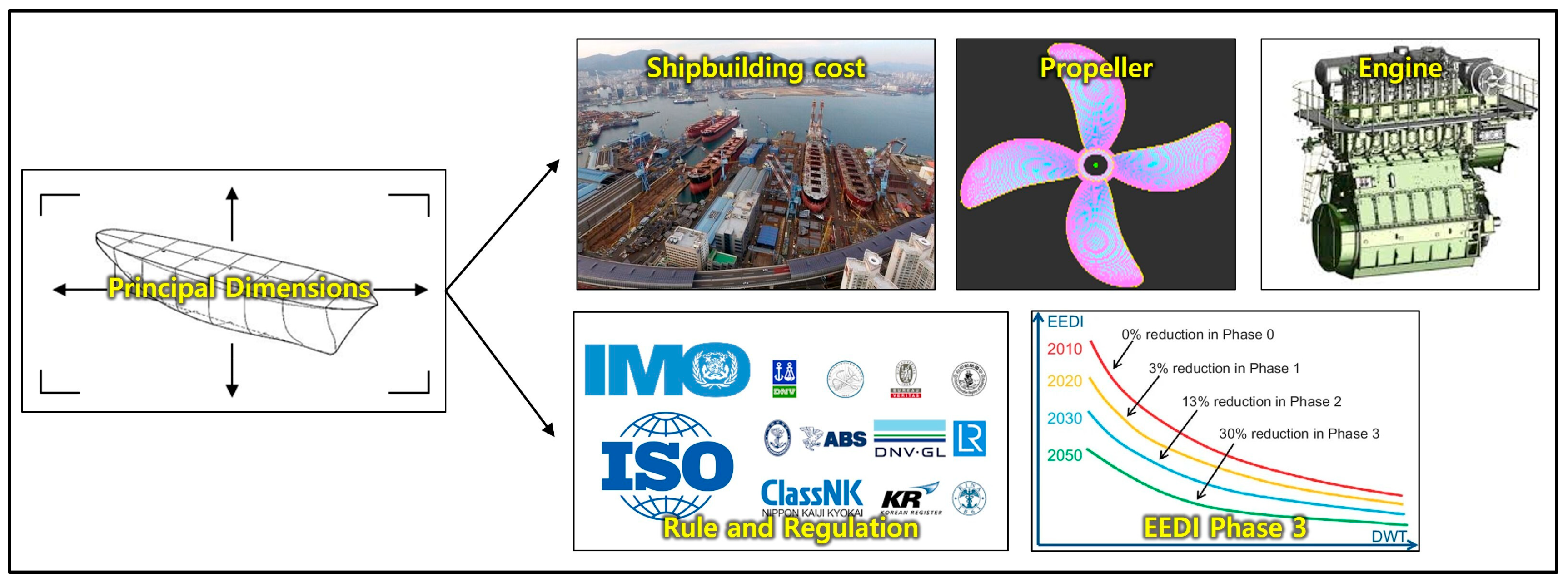
The maritime industry accounts for approximately 90% of global trade volume, playing a vital role in economic development. Since 99.7% of South Korea’s import and export cargo is transported by sea, the maritime industry has an immense impact on the national economy. However, as the maritime industry is responsible for approximately 3% of global CO₂ emissions, the International Maritime Organization (IMO) has introduced various regulations and guidelines to reduce carbon emissions [1,2]. At the 62nd session of the Marine Environment Protection Committee (MEPC), the IMO introduced the Energy Efficiency Design Index (EEDI) [3], which quantifies the energy efficiency of a ship by representing the amount of CO₂ emitted per tonne of cargo transported per nautical mile. Since EEDI serves as the mandatory minimum efficiency standard that all newbuild vessels must comply with, it is a critically important indicator at the ship design stage. As shown in Figure 1, EEDI is closely related to the principal dimensions of the ship, engine performance, and propulsion system efficiency, and is therefore regarded as an important indicator not only from an environmental perspective but also from an economic standpoint. Furthermore, the determined principal dimensions directly affect shipbuilding cost, propeller performance, and main engine performance, and must comply with the rules and regulations of various international classification societies. Therefore, it is of critical importance for ship owners and naval architects to determine the optimal principal dimensions at the design stage to maximize energy efficiency while minimizing operating costs.

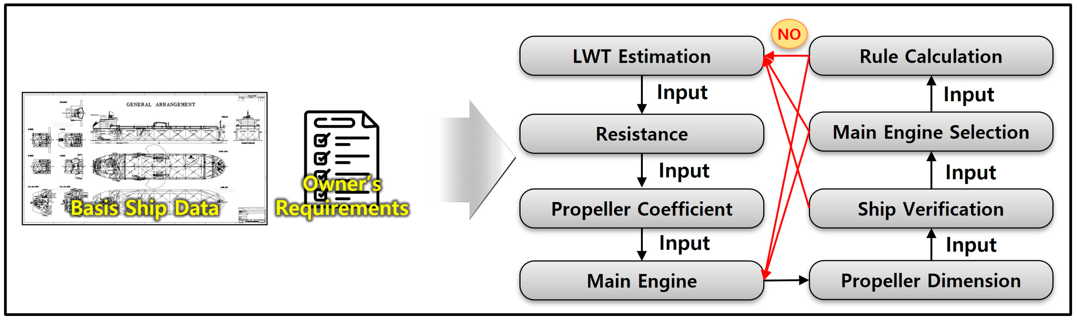
However, as illustrated in Figure 2, the determination of principal dimensions in the early ship design stage requires iterative calculations based on the basis ship particulars and ship owner’s requirements, and involves a complex process in which, if the design constraints are not satisfied, the procedure must revert to a previous step. This not only consumes significant manpower and time but also poses a high risk of substantial loss of time and money, as strengthened environmental regulations such as EEDI Phase 3 directly affect all aspects of the design [4], including principal dimensions, propulsion system, and Main Engine Selection. Furthermore, due to time constraints, there is an inherent limitation in the designer’s ability to explore a sufficiently large number of design alternatives.

Therefore, this study develops a program to automate the determination of principal dimensions in the early design stage and to derive the optimal $L_{BP}$ (Length Between Perpendiculars), Breadth, Depth, and $C_B$ (Block Coefficient) that satisfy EEDI Phase 3 requirements while maximizing operational efficiency and economic feasibility, by applying the NSGA-II (Non-Dominated Sorting Genetic Algorithm) to a VLSFO/LNG dual-fuel Aframax Tanker.

1.2. Related Studies

Previous studies on the optimization of principal dimensions in the early ship design stage are summarized as follows. Chen et al. [5] optimized the principal dimensions of a ship by applying fuzzy decision-making theory, with manufacturing cost, annual cargo capacity, payback period, and net present value defined as objective functions. Park et al. [6] performed optimization with minimum shipbuilding cost as the objective function by simultaneously considering the determination of principal dimensions and the hull form variation process during early ship design. Park et al. [7] conducted principal dimension optimization of a small catamaran to minimize total resistance using the SHERPA algorithm in HEEDS, an AI-based design search technique.

Previous studies on the optimization of principal dimensions considering EEDI are summarized as follows. Wang et al. [8] determined the optimal principal dimensions to minimize EEDI using PSO (Particle Swarm Optimization), MIGA (Multi-Island Genetic Algorithm), and ASA (Adaptive Simulated Annealing Algorithm), taking into account flow velocity, wetted surface area, and total resistance coefficient. Xie et al. [9] determined the optimal principal dimensions to minimize EEDI for a 7500 DWT bulk carrier using the DAPS (P-system based Diffusion Algorithm).

In addition to the studies described above, various optimization approaches have been applied to broader ship design problems in recent years, including hull form optimization [10,11,12], operational efficiency improvement [13], ship arrangement design [14,15], and hydrodynamic performance analysis based on principal dimensions [16,17]. Furthermore, optimization methods have been extended to ship operational problems and early-stage design, including tugboat operation planning, surrogate model-based system design, and multi-objective optimization of ship main dimensions [18,19,20,21,22]. Reviews of these methodologies have also been systematically conducted to analyze research trends in ship design optimization [23,24,25,26].

A comparison of the present study with previous research is summarized in

Table 1. Comparison of our study with previous research on ship principal dimension optimization.

Reference	Algorithm	Objective Function	EEDI Treatment	Automation	Dual Fuel
Chen et al. [5]	Fuzzy Decision-Making (FCE)	Building cost, ATC, PBP, NPV	X	X	X
Park et al. [6]	Collaborative Optimization (CO)	Minimize building cost	X	△	X
Park et al. [7]	SHERPA (HEEDS)	Minimize total resistance	X	△	X
Wang et al. [8]	PSO/MIGA/ASA/NSGA-II	Minimize EEDI	O	X	X
Xie et al. [9]	DAPS (P-system-based Diffusion Algorithm)	Minimize EEDI	O	X	X
This study	NSGA-II	Minimize RT, SFOC, LWT	Phase 3	O	O

Note: O = considered; X = not considered; △ = partially considered.

. Most existing studies have focused on minimizing shipbuilding cost or addressing a single environmental regulation objective. Research on design automation that simultaneously considers resistance performance, fuel efficiency, and construction economics under the strengthened EEDI Phase 3 remains insufficient. To address these limitations, this study develops an automated early design optimization system that integrates the principal dimension calculation process—including lightweight (LWT) estimation, Main Engine Calculation, and Propeller Dimension Calculation—with the constraint calculation process required to satisfy EEDI Phase 3 and minimum freeboard requirements. In particular, the system accurately computes the Attained EEDI reflecting the characteristics of a VLSFO/LNG dual-fuel system and aims to effectively derive the optimal solution among conflicting objective functions using the NSGA-II algorithm.

2. Calculation Process During the Early Design Stage of a Ship

The early ship design stage is a complex process that must simultaneously satisfy the required DWT and service speed $V_s$ while considering economic feasibility, operational efficiency, and regulatory compliance. This section describes the eight Calculation Modules required to determine the principal dimensions of a ship and the two Calculation Modules required for constraint evaluation.

2.1. Overall Calculation Process

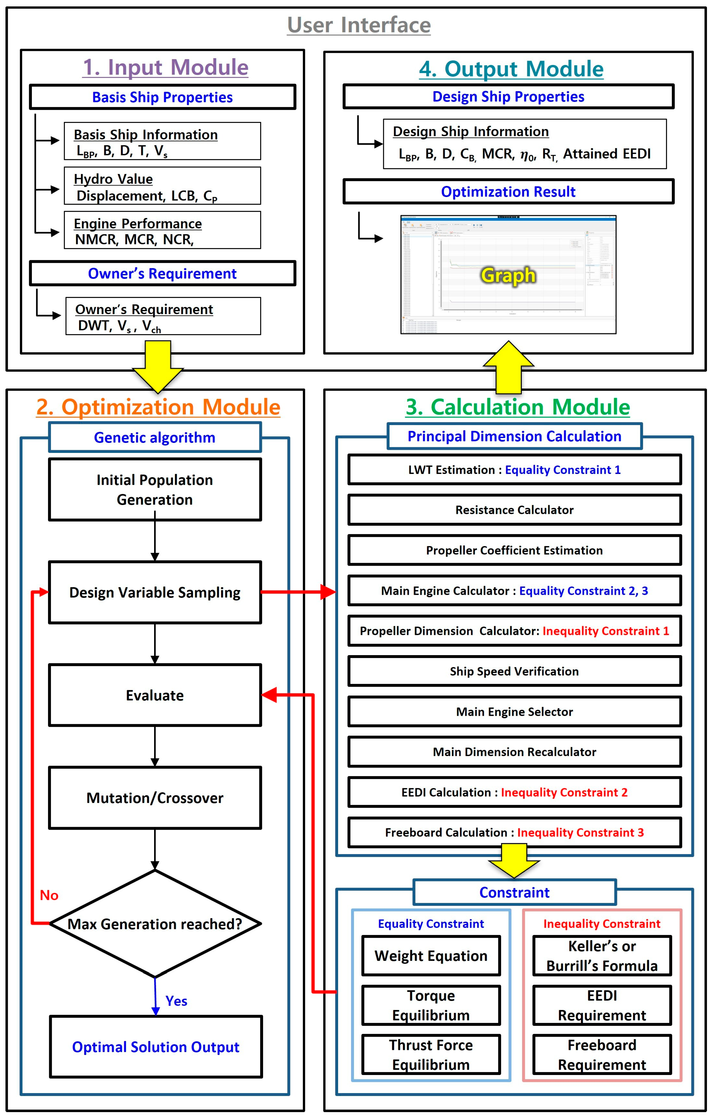
The ship principal dimension optimization system developed in this study consists of four modules—the Input Module, Optimization Module, Calculation Module, and Output Module—as shown in Figure 3. The functions of each module and the information flow between modules are described as follows.

(1) Input Module: The Input Module receives two types of information from the user. First, the principal dimensions of the basis ship, hydrodynamic coefficients, and propeller and main engine information are entered, together with the ship owner’s requirements. The input information is then passed to the Optimization Module.

(2) Optimization Module: The Optimization Module employs an NSGA-II based genetic algorithm to search for the optimal design variables. Based on the information received from the Input Module, an initial population is generated, and at each generation, the design variables—the initial principal dimensions—are sampled and passed to the Calculation Module. After verifying the objective function values and constraint violations returned from the Calculation Module, selection, crossover, and mutation operations are iteratively performed. When the maximum number of generations is reached, the optimal solution is passed to the Output Module.

(3) Calculation Module: The Calculation Module sequentially executes ten sub-modules using the design variables received from the Optimization Module and the information provided through the Input Module. The LWT Estimation sub-module computes a preliminary estimate of the initial principal dimensions from the design variables using weight equation. The Resistance Calculator sub-module computes the hull resistance from the estimated principal dimensions, and the Propeller Coefficient Estimation sub-module estimates propeller coefficients including wake fraction and thrust deduction factor. The Main Engine Calculator sub-module applies torque equilibrium and thrust force equilibrium to determine the required delivered power and shaft rotational speed, while the Propeller Dimension Calculator sub-module determines the propeller diameter, pitch ratio, and expanded area ratio satisfying the empirical criteria of Keller and Burrill. The Ship Speed Verification sub-module verifies the ship speed based on the determined propeller dimensions, and the Main Engine Selector sub-module selects the main engine with the minimum SFOC that satisfies the engine layout boundary conditions.

The Main Dimension Recalculator sub-module recalculates the principal dimensions reflecting the NMCR of the finally selected main engine. After the eight principal dimension calculation sub-modules are executed, two additional sub-modules for constraint evaluation are executed independently. The EEDI Calculation sub-module computes the Attained EEDI based on the final principal dimensions and the selected engine and determines whether EEDI Phase 3 compliance is satisfied. The Freeboard Calculation sub-module evaluates the adequacy of the actual freeboard relative to the required freeboard, in accordance with ICLL 1966. The results from the eight principal dimension sub-modules are returned to the Optimization Module as objective function values, and the results from the two constraint sub-modules are returned as constraint violation indicators.

(4) Output Module: Upon completion of optimization, the Output Module displays the design ship particulars and information such as Attained EEDI corresponding to the optimal solution and provides the user with a graphical visualization of the objective function values and constraint violations.

The details of the calculation method for each sub-module within the Calculation Module are briefly described in the following sections. For further details, the reader is referred to Roh et al. [27].

2.2. LWT Estimation

In the early design stage, very little data is available to determine the principal dimensions; therefore, initial values are estimated from the basis ship. The LWT Estimation module applies the weight equation to determine the initial principal dimensions.

$$\rho \cdot L\cdot B\cdot T\cdot C_B\cdot (1+\alpha )=DWT+LWT$$

(1)

The LWT value is estimated by applying Method 4 of the weight equation proposed by Roh et al. [27], which divides the lightweight function into steel weight (W_s), outfitting weight (W_o) and machinery weight (W_m). The steel weight is defined as a function of Length (L), Breadth (B), and Depth (D); the outfitting weight is defined as a function of Length and Breadth; and the machinery weight is defined as a function of NMCR. Here, C_s, C_o, and C_m are empirical coefficients for estimating the steel, outfitting, and machinery weights, respectively, and NMCR denotes the Nominal Maximum Continuous Rating (kW).

$$\begin{array}{l}LWT=W_s+W_o+W_m=C_s\cdot L^{1.6}\cdot (B+D)+C_o\cdot L\cdot B+C_m\cdot NMCR\\ \hspace{0.17em}\hspace{0.17em}\hspace{0.17em}\hspace{0.17em}\hspace{0.17em}\hspace{0.17em}\hspace{0.17em}\hspace{0.17em}\hspace{0.17em}\hspace{0.17em}\hspace{0.17em}\hspace{0.17em}\hspace{0.17em}\hspace{0.17em}\hspace{0.17em}\hspace{0.17em}\hspace{0.17em}\hspace{0.17em}\hspace{0.17em}\hspace{0.17em}\hspace{0.17em}\hspace{0.17em}\hspace{0.17em}\hspace{0.17em}\hspace{0.17em}\hspace{0.17em}\hspace{0.17em}=L^{1.6}\cdot (B+D)+C_o\cdot L\cdot B+C_{power}\cdot {(L\cdot B\cdot T\cdot C_B\cdot (1+\alpha ))}^{2/3}\cdot V_s^3\end{array}$$

(2)

Since the NMCR of the main engine is not yet determined at the early design stage, the Delivered Horsepower (DHP) is first estimated as a function of displacement $(\Delta )$ and ship speed $(V_S)$. Assuming that DHP is proportional to ${\Delta }^{2/3}$ and $V_s^3$, the DHP can be expressed as Equation (3):

$$DHP={\displaystyle \frac{{\Delta }^{2/3}\cdot V_S^3}{C_{ad}}}$$

(3)

where $C_{ad}$ is the admiralty coefficient, defined as Equation (4), which can be regarded as a measure of the propulsive efficiency of the ship.

$$C_{ad}={\displaystyle \frac{DHP}{{\Delta }^{2/3}\cdot V_s^3}}$$

(4)

Substituting the weight equation into Equation (3), the DHP can be rewritten as Equation (5).

$$DHP={\displaystyle \frac{{(\rho \cdot L\cdot B\cdot T\cdot C_B\cdot (1+\alpha ))}^{2/3}\cdot V_s^3}{C_{ad}}}$$

(5)

The NMCR is then estimated by DHP by incorporating the sea margin, engine margin, derating ratio, and transmission efficiency as follows:

$$NMCR=C_1\cdot DHP={\displaystyle \frac{C_1}{C_{ad}}}\cdot {(\rho \cdot L\cdot B\cdot T\cdot C_B\cdot (1+\alpha ))}^{2/3}\cdot V_s^3$$

(6)

where $C_1=(1/{\eta }_T)\cdot (1+\mathrm{Sea}\hspace{0.17em}\mathrm{Margin}/100)\cdot (1/\mathrm{Engine}\hspace{0.17em}\mathrm{Margine})\cdot (1/\mathrm{Derating}\hspace{0.17em}\mathrm{Ratio})$ and ${\eta }_T$ is the transmission efficiency. Substituting Equation (6) into the machinery weight equation $W_m=C_m\cdot NMCR$, the coefficient $C_{power}$ in Equation is defined as $C_{power}=C_m\cdot C_1/C_{ad}$.

2.3. Resistance Calculation

To compute the effective horsepower (EHP) of the design ship, the Holtrop–Mennen method [28,29] is applied to predict the total resistance (R_T). The resistance prediction formula proposed by Holtrop–Mennen is as given in Equation (7). Here, the equation elements are defined as follows: frictional resistance (R_F), wave-making resistance (R_w), bulbous bow resistance (R_B), transom stern resistance (R_TR), model–ship correlation resistance (R_A), and total resistance (R_T); the latter is computed as the sum of these components.

$$R_T=R_F(1+k_1)+R_{APP}+R_W+R_B+R_{TR}+R_A$$

(7)

In this study, a correction factor was derived by comparing the resistance value of the basis ship computed via Holtrop–Mennen with the actual resistance value obtained from the basis ship’s actual power, and the resistance was interpolated using this correction factor.

$$R_{T,design}={\displaystyle \frac{R_{T,design,Holtrop\hspace{0.17em}\&\hspace{0.17em}Mennen}}{R_{T,basis,Holtrop\hspace{0.17em}\&\hspace{0.17em}Mennen}}}\cdot R_{T,basis}$$

(8)

2.4. Propeller Coefficient Estimation

This module receives the basis ship particulars and propeller information as input and estimates the wake fraction (w) and thrust deduction factor (t) by accounting for the interaction between the hull and the propeller. This process also computes propulsive efficiency (${\eta }_D$) and relative rotative efficiency (${\eta }_R$). The calculations are performed using the Approximation Formula of Propeller Efficiency proposed by Holtrop–Mennen. The estimation formula for propeller diameter ($D_p$) is as given in Equation (9). Here, $P_{MCR}$ is the power under MCR (Maximum Continuous Rating) conditions, $n_{MCR}$ is the propeller rotational speed (rpm) under MCR conditions, and $c_1$ is a correction factor to account for the difference in draft between the design ship and the basis ship.

$$D_p=15.4\times {({\displaystyle \frac{P_{MCR}}{n_{MCR}^3}})}_{basisship}^{0.2}\times c_1$$

(9)

The estimation formula for relative rotative efficiency (${\eta }_R$) is as given in Equation (10). Here, $A_E/A_O$ denotes the expanded area ratio, $C_P$ is the prismatic coefficient, $lcb$ is the longitudinal center of buoyancy, $P_i$ is the propeller pitch, and $n_{shaft}$ is the number of propeller shafts.

$${\eta }_R=\left(\begin{array}{c}0.9922-0.05908A_E/A_o+0.07424(C_P-0.0225lcb)\hspace{0.17em}\hspace{0.17em}\mathrm{when}\hspace{0.17em}{n}_{shaft\hspace{0.17em}}=1\\ 0.9737+0.111(C_P-0.0225lcb)-0.06325P_i/D_P)\hspace{0.17em}\hspace{0.17em}\hspace{0.17em}\hspace{0.17em}\mathrm{when}\hspace{0.17em}{n}_{shaft\hspace{0.17em}}=2\end{array}\right.$$

(10)

The estimation formula for wake fraction (w) is as given in Equation (11). Here, $C_9$ and $C_{11}$ are empirical coefficients of Holtrop–Mennen determined based on the stern form, $C_v$ is the viscous resistance coefficient, $T_A$ is the stern draft, $C_{P1}$ is the modified prismatic coefficient, and $C_{stern}$ is a coefficient depending on the stern cross-section shape, taking values of −10 for V-shaped sterns, 0 for normal sterns, and +10 for U-shaped sterns.

$$\begin{array}{l}w=C_9\cdot C_v{\displaystyle \frac{L}{T_A}}(0.661875+1.21756C_{11}{\displaystyle \frac{C_v}{(1-C_{P1})}})\\ \hspace{0.17em}\hspace{0.17em}\hspace{0.17em}\hspace{0.17em}\hspace{0.17em}\hspace{0.17em}+0.24558\sqrt{{\displaystyle \frac{B}{L(1-C_{P1})}}}-{\displaystyle \frac{0.09726}{0.95-C_p}}+{\displaystyle \frac{0.11434}{0.95-C_B}}\\ \hspace{0.17em}\hspace{0.17em}\hspace{0.17em}\hspace{0.17em}\hspace{0.17em}\hspace{0.17em}+0.75C_{stern}\cdot C_v+0.002C_{stern}\end{array}$$

(11)

The estimation formula for thrust deduction factor (t) is as given in Equation (12). Here, $L_{WL}$ is the Length at the waterline, $C_{10}$ is an empirical coefficient of Holtrop–Mennen determined by the stern form, D is the molded depth, and T is the design draft.

$$\begin{array}{l}t=0.001979L_{WL}/(B-B\cdot C_{P1})+1.0585C_{10}\\ \hspace{0.17em}\hspace{0.17em}\hspace{0.17em} \hspace{0.17em}-0.00524-0.1418D^2/(B\cdot T)+0.0015C_{stern}\end{array}$$

(12)

2.5. Propeller and Main Engine Selection

The propeller dimension determination and Main Engine Selection process consists of three stages. Each stage receives the output of the previous stage as input, and all stages are based on two common equilibrium conditions. The first condition is the torque equilibrium condition, which requires that the torque transmitted by the diesel engine through the shaft equals the torque absorbed by the propeller. Here, $P=\mathrm{DHP}\cdot {\eta }_R$.

$${\displaystyle \frac{P}{2\pi n}}=\rho \cdot n^2\cdot D_P^5\cdot K_Q$$

(13)

The second condition is the thrust force equilibrium condition, which requires that the thrust generated by the propeller overcomes the total resistance of the ship at the given speed. Here, $t$ is the thrust deduction factor.

$${\displaystyle \frac{R_T}{1-t}}=\rho \cdot n^2\cdot D_P^2\cdot K_T$$

(14)

2.5.1. Main Engine Caculation

This stage receives the propeller diameter $(D_P)$, expanded area ratio $(A_E/A_o)$, number of blades $(z)$, ship speed $(V_s)$, and total resistance $(R_T)$ as input, and determines the delivered power $(P)$, shaft rotational speed $(n)$, and pitch $(P_i)$ that simultaneously satisfy both equilibrium conditions while maximizing the propeller open water efficiency. By transforming the second equilibrium condition into the form $K_T=c_2{J}^2$, Equation (15) is obtained.

$$c_2={\displaystyle \frac{R_T}{(1-t)\cdot \rho \cdot D_P^2\cdot V_A^2}}$$

(15)

Substituting Equation (15) into the open water performance curve (POW curve) of the B-series propeller, the advance coefficient $J_x$ and the corresponding $K_{T,x},\hspace{0.17em}{K}_{Q,x}$ that maximize the propeller open water efficiency ${\eta }_0={\displaystyle \frac{J}{2\pi }}\cdot {\displaystyle \frac{K_T}{K_Q}}$ are identified across multiple pitch ratios ($P_i/D_P$). From these, the main engine rotational speed ($n_x=V_A/(D_P\cdot J_x)$) and delivered power $P_x=2\pi \rho n_x^3{D}_P^5{K}_{Q,x}$ are determined. BHP, NCR, MCR, and the corresponding rotational speeds $n_{NCR},n_{MCR}$ are then computed, and it is verified that the MCR and NCR points fall within the engine layout diagram.

2.5.2. Propeller Dimension Calculation

Once the propeller design point is determined, this stage receives the number of blades and total resistance at each speed as input, and optimizes the propeller diameter $(D_P)$, pitch $(P_i)$, expanded area ratio $(A_E/A_o)$, and ship speed $(V_s)$. In the Propeller Dimension Calculation, a third constraint is added to prevent cavitation using the empirical criteria of Keller and Burrill. The Keller minimum area ratio formula is as given in Equation (16).

$$A_E/A_o=K+{\displaystyle \frac{(1.3+0.3z)\cdot T}{D_p^2\cdot (p_0+\rho g{h}^{\ast }-p_v)}}$$

(16)

Here, K is 0.2 for a single-screw vessel and 0.1 for a twin-screw vessel, h^* (equation) is the shaft immersion depth, and (equation) (seawater at 15 °C). The Burrill minimum area ratio formula is as given in Equation (17).

$$\begin{array}{l}{A}_E/A_o\ge F\cdot {\displaystyle \frac{{\eta }_0/{(1/J)}^2}{\{1+4.826{(1/J)}^2\}\cdot (1.067-0.229\cdot P_i/D_P)}}\\ F={\displaystyle \frac{{\eta }_R\cdot B_P^2\cdot V_A^{1.25}}{287.4{(10.18+h)}^{0.625}}},\hspace{0.17em}\hspace{0.17em}\hspace{0.17em}\hspace{0.17em}{B}_P=n\cdot P^{0.5}/V_A^{2.5}\end{array}$$

(17)

Starting from an initial expanded area ratio $(A_E/A_o)$ of 0.4 and incrementing by 0.05, the ship speed $(V_s)$ is computed at each expanded area ratio $(A_E/A_o)$; then, the minimum expanded area ratio simultaneously satisfying the second and third conditions, together with the corresponding ship speed $(V_s)$, propeller diameter $(D_P)$, and pitch $(P_i)$, are determined.

2.5.3. Ship Speed Verification

Using the principal propeller dimensions computed by the Propeller Dimension Calculator, this verification stage simultaneously solves the two equilibrium conditions to compute the engine power and shaft rotational speed at the actual ship speed. This stage is computed by solving a system of two nonlinear equations with two unknowns (P, n). By transforming the second equilibrium condition into the form ${\displaystyle \frac{K_T}{J^2}}=c_2$, the advance coefficient J is first determined, from which the rotational speed ($n={\displaystyle \frac{V_A}{(J\cdot D_P)}}$) is computed, and DHP, BHP, NCR, and MCR are then sequentially calculated.

2.5.4. Main Engine Selection

Once the delivered power and rotational speed of the design ship are determined, the main engine is selected based on these values. For each engine in the engine list, engine boundaries are generated for each number of cylinders $(S_y)$, and engines are selected by verifying that the propeller design point $(n_x,P_{NCR})$, MCR point, and NCR point all fall within the boundary of the corresponding engine layout diagram. Among the eligible engines, the engine with the lowest SFOC is selected as the main engine to satisfy the EEDI requirements. A partial list of the engines used in this study is presented in

Table 2. Engine list (partial).

Maker	Engine Model	No. of Cylinder	P1 (kW)	P2 (kW)	P3 (kW)	P4 (kW)	SFOC (g/kWh)	GI
WinGD	X40DF-1.0	5~8	555	665	780	935	189.6	1
	X52DF	5~8	930	1120	1240	1490	184.1	1
	X72DF	5~8	2080	2500	2685	3225	182	1
	X82-2.0	6~9	2490	2980	3600	4320	176.9	0
	X82DF-2.0	6~9	2490	2980	3600	4320	176.9	1
Man B&W	S60ME-C10.7	5~8	1470	1950	1880	2490	166	0
	S50ME-C9.7	5~9	970	1290	1340	1780	168	1
	G60ME-C10.5	5~8	1500	1990	2140	2840	167	1
	G70ME-C10.7	5~6	2080	2760	2840	3770	166	0
	G95ME-C10.5	5~12	4520	6010	5170	6870	161	1

.

2.6. Main Dimension Recalculation

The initial principal dimensions are re-estimated by employing the preliminary principal dimensions and the NMCR of the selected main engine as input. The recalculation is performed using Method 4 of the weight equation proposed by Roh et al. [27], which was also applied in the LWT Estimation module.

$$LWT=W_s+W_o+W_m=C_s\cdot L^{1.6}\cdot (B+D)+C_o\cdot L\cdot B+C_m\cdot NMCR$$

(18)

2.7. EEDI Calculation

In accordance with the IMO’s carbon emission regulations [3,4], accurate EEDI Calculation is essential to ensure mandatory compliance with EEDI Phase 3. The formula for the Required EEDI is as given in Equation (19).

$$\mathrm{Required}\hspace{0.17em}\mathrm{EEDI}\hspace{0.17em}=\hspace{0.17em}(1-{\displaystyle \frac{x}{100}})\times a\times b^{-c}\left\{\begin{array}{c}x=\mathrm{Reduction}\hspace{0.17em}\mathrm{Factor}\\ a=\hspace{0.17em}\mathrm{constant}\hspace{0.17em}\mathrm{of}\hspace{0.17em}\mathrm{the}\hspace{0.17em}\mathrm{ship}\hspace{0.17em}\mathrm{type}\\ b=\mathrm{DWT}\hspace{0.17em}\mathrm{of}\hspace{0.17em}\mathrm{the}\hspace{0.17em}\mathrm{ship}\end{array}\right.$$

(19)

The formula for the Attained EEDI used in this study is as given in Equation (20), and the definitions of the parameters used are presented in

Table 3. Descriptions of different parameters of Attained EEDI.

Parameter	Description
$f_j$	Correction factor to account for ship-specific design elements (e.g., ice class ships, shuttle tankers)
PME	75% of the main engine MCR (Maximum Continuous Rating) in kW
fDFgas	Fraction of gas fuel used for dual fuel engines
CF_Pilotfuel	Carbon conversion factor for pilot fuel
SPOCME	Specific pilot fuel oil consumption of ME
CF_LNG	Carbon conversion factor for LNG
SGCME_LNG	Specific gas consumption of ME using LNG
fDF_liquid	Fraction of liquid fuel used for dual fuel engines
CF_VLSFO	Carbon conversion factor for VLSFO
SFOCVLSFO	Specific fuel oil consumption of VLSFO
PAE	Auxiliary engine power
CF_MGO	Carbon conversion factor for MGO
SFOCAE_MGO	Specific fuel oil consumption of AE using MGO
$f_i$	Correction factor for ship-specific design elements (e.g., ice class)
$f_c$	Cubic capacity correction factor (for chemical/gas carriers)
$f_w$	Coefficient for speed decrease in representative sea conditions
$f_{i\text{\_}CSR}$	Correction factor for bulk carriers and oil tankers
$V_{ref}$	Ship speed in nautical miles per hour at PME
Capacity	Computed as a function of deadweight

.

$$\mathrm{Attained}\hspace{0.17em}\mathrm{EEDI}={\displaystyle \frac{\begin{array}{l}{f}_j\times (P_{ME}\times (f_{DFgas}\times (C_{F\text{\_}Pilotfuel}\times SPO{C}_{ME}+C_{F\text{\_}LNG}\times SG{C}_{ME\text{\_}LNG})\\ +f_{DF\text{\_}liquid}\times C_{F\text{\_}VLSFO}\times SFO{C}_{VLSFO})+P_{AE}\times C_{F\text{\_}MGO}\times SFO{C}_{AE\text{\_}MGO})\end{array}}{f_i\times f_c\times f_w\times f_{i\text{\_}CSR}\times V_{ref}\times Capacity}}$$

(20)

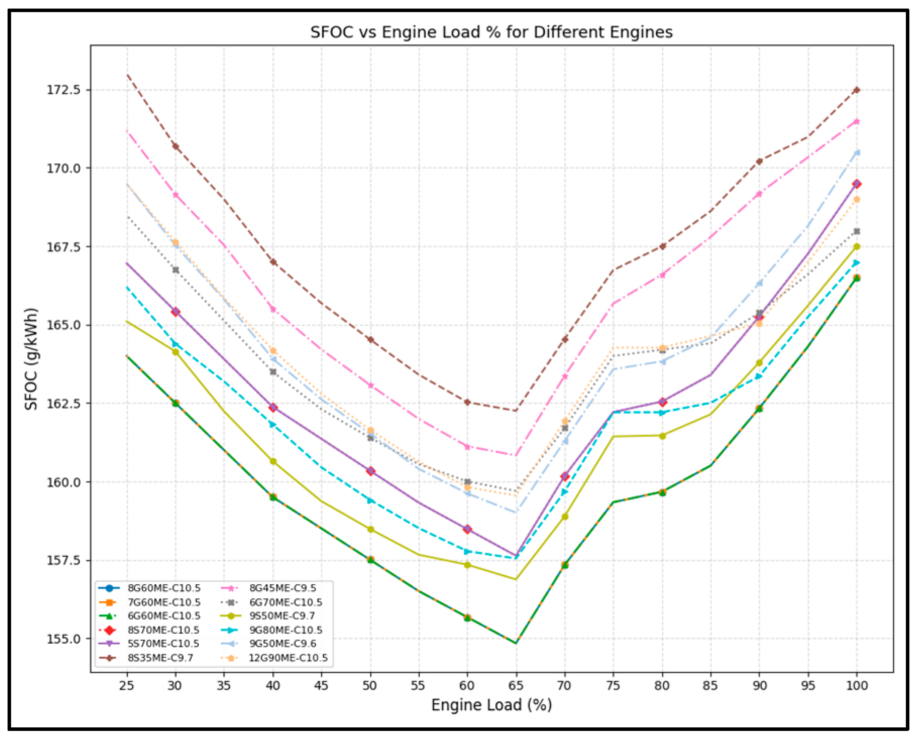
To compute the Attained EEDI, SFOC values at each engine load are required. However, in most cases, only the SFOC value at 100% load is provided for a given engine. Therefore, in this study, SFOC values at various engine loads were compared across multiple engines, confirming that most engines exhibit a similar variation pattern. The average rate of change was computed, and SFOC values at each engine load were estimated through regression analysis. The SFOC values by engine load for each engine are presented in Figure 4.

The results computed through regression analysis were compared with those obtained from the MAN B&W calculation program, revealing a discrepancy of approximately 1–2 g/kWh. A comparison of the MAN B&W results and the values computed by the program developed in this study is presented in

Table 4. Comparison of SFOC values between MAN B&W calculation and regression analysis results.

Engine Load (%)	Program (Regression)	MAN B&W (ISO, NCR)	Difference
100	166.00	166.00	0.00
88.22	161.47	161.30	+0.17
75	159.92	159.50	+0.42
50	157.70	159.00	−1.3

.

2.8. Freeboard Calculation

The Freeboard Calculation receives basis ship information—including the freeboard Length and waterplane area of the basis ship—and the determined initial principal dimensions of the design ship as input. The formula for the required freeboard is as given in Equation (21), and the definitions of the parameters used are presented in

Table 5. Description of Freeboard Equation.

Parameter	Description
Ft	Calculation of tabular freeboard
Ccb	Calculation of the addition for Block Coefficient
CD	Calculation of the correction for Depth
CDL	Calculation of the correction for position of deck line
CST	Calculation of the deduction for superstructures and trunks
Cs	Calculation of the correction for sheer
CBH	Calculation of the addition for minimum bow height
Df	Freeboard Depth
Ts	Scantling draft

.

$$F{b}_s=F_t+c_{cb}+c_D+c_{DL}-c_{ST}+c_s+c_{BH}$$

(21)

The formula for the actual freeboard is as given in Equation (22).

$$F_a=D_f-T_s$$

(22)

3. Optimization Problem Formulation

3.1. Problem Definition

The determination of optimal principal dimensions in the early ship design stage is a critical process for simultaneously ensuring economic feasibility and operational efficiency. As described in Section 2, the design ship’s principal dimensions are determined by sequentially executing the ten sub-modules of the Calculation Module, based on the basis ship information and ship owner’s requirements entered through the Input Module. In this study, the early design problem is formulated as a multi-objective optimization problem to maximize economic feasibility in terms of both construction and operation while complying with the strengthened international maritime regulation of EEDI Phase 3.

3.2. Design Variables

As described in Section 2.1, the Optimization Module samples design variables at each generation and passes them to the Calculation Module. In this study, four principal dimensions that directly affect the propulsion performance and economic feasibility of the ship are defined as design variables: Length Between Perpendiculars ($L_{BP}$), Breadth, Depth, and Block Coefficient ($C_B$).

$$X=(L_{BP},B,D,C_B)$$

(23)

3.3. Objective Functions

In this study, three objective functions are minimized to simultaneously ensure economic feasibility and operational efficiency. The first objective function minimizes the SFOC (specific fuel oil consumption) of the main engine selected in the Main Engine Selection module (Section 2.5.4), to secure operational economy. SFOC represents the quantity of fuel consumed per unit power output per hour, and its minimization can significantly reduce the substantial operating costs incurred during ship operation. The second objective function minimizes the lightweight (LWT) to reduce shipbuilding costs through savings in steel weight. Finally, the total resistance computed by the Holtrop–Mennen method in the Resistance Calculation Module (Section 2.3) is minimized to maximize propulsive efficiency. As the solution space of the objective functions becomes more complex depending on the combination of design variables, the NSGA-II algorithm, which is well-suited for deriving global optimal solutions, is applied to perform the multi-objective optimization. Each objective function is individually scaled by a normalization factor and a weight coefficient as follows:

$$f_1=w_1\times {\displaystyle \frac{R_T}{R_{T,ref}}},\hspace{0.17em}{f}_2=w_2\times {\displaystyle \frac{\mathrm{SFOC}}{{\mathrm{SFOC}}_{ref}}},\hspace{0.17em}{f}_3=w_3\times {\displaystyle \frac{\mathrm{LWT}}{{\mathrm{LWT}}_{ref}}}$$

(24)

The weight coefficients $w_1,w_2,w_3$ are adjusted to reflect different design priorities. Four representative cases are defined as summarized in

Table 6. Weight combinations for each optimization case.

Case	${\mathit{w}}_1({\mathit{R}}_{\mathit{T}})$	${\mathit{w}}_2(\mathbf{S}\mathbf{F}\mathbf{O}\mathbf{C})$	${\mathit{w}}_3(\mathbf{L}\mathbf{W}\mathbf{T})$
Case 1	0.33	0.33	0.33
Case 2	0.50	0.25	0.25
Case 3	0.25	0.50	0.25
Case 4	0.25	0.25	0.50

, and a detailed description of each case is provided in Section 4.2.

3.4. Constraints

The constraints imposed in the optimization consist of equality constraints to maintain physical equilibrium, and inequality constraints to ensure regulatory compliance and safety.

3.4.1. Equality Constraint

The first equality constraint is the weight equilibrium equation. Based on the weight equation of the LWT Estimation described in Section 2.2, the displacement must equal the total weight of the ship for the vessel to be in static equilibrium in the design draft. This is expressed as the corresponding Equation (25).

$$\rho \cdot L\cdot B\cdot T\cdot C_B\cdot (1+\alpha )=LWT+DWT$$

(25)

The second equality constraint is the torque equilibrium condition. The torque transmitted from the main engine through the shaft must equal the torque absorbed by the propeller rotating in the fluid, which corresponds to the first condition in Section 2.5.1. This is expressed as the corresponding Equation (26).

$${\displaystyle \frac{P}{2\pi n}}=\rho \cdot n^2\cdot D_P^5\cdot K_q\hspace{0.17em}(\mathrm{where},\hspace{0.17em}P=DHP\cdot {\eta }_R)$$

(26)

The third equality constraint is the thrust force equilibrium condition. The thrust generated by the propeller must overcome the total resistance of the ship to maintain a given speed, which corresponds to the second condition in Section 2.5.1. This is expressed as the corresponding Equation (27).

$${\displaystyle \frac{R_T}{1-t}}=\rho \cdot n^2\cdot D_P^2\cdot K_T$$

(27)

3.4.2. Inequality Constraint

The first inequality constraint requires that the minimum area ratio condition be satisfied to prevent cavitation, corresponding to the third condition in Section 2.5.2. In this study, the minimum area ratio is constrained using the empirical criteria of Keller [30] and Burrill [31], as expressed in Equations (28) and (29), respectively.

$$A_E/A_o\ge K+{\displaystyle \frac{(1.3+0.3z)\cdot T}{D_P^2\cdot (p_0+\rho g{h}^{\ast }-p_v)}}$$

(28)

$$A_E/A_o\ge {\displaystyle \frac{F({\eta }_0/{(1/J)}^2)}{{(1+4.826{(1/J)}^2)}^{0.375}\times (1.067-0.229\cdot P_i/D_p)}}$$

(29)

The second inequality constraint is the EEDI compliance condition. The Attained EEDI computed through the EEDI Calculation described in Section 2.7 must not exceed the Required EEDI. In accordance with IMO’s carbon emission regulations, all newbuild vessels must comply with EEDI Phase 3. This is expressed as the corresponding Equation (30).

$$\mathrm{Required}\hspace{0.17em}\mathrm{EEDI}\hspace{0.17em}\ge \hspace{0.17em}\mathrm{Attained}\hspace{0.17em}\mathrm{EEDI}$$

(30)

The third inequality constraint is the freeboard constraint. The actual freeboard ($F_a$) computed through the Freeboard Calculation described in Section 2.8 must exceed the required freeboard ($F_b$) stipulated by ICLL 1966. This is expressed as the corresponding Equation (31).

$$F_a\ge F_b$$

(31)

4. Applications

4.1. Early-Stage Ship Principal Dimension Optimization Program Considering EEDI

In this study, a GUI (Graphical User Interface)-based program was developed to receive basis ship information and the ship owner’s requirements as input and perform the optimization. The overall system configuration is as shown in Figure 3, and the program consists of four sub-modules.

The NSGA-II algorithm [32] is an elitist multi-objective genetic algorithm that maintains solution diversity through non-dominated sorting and crowding distance calculation. The optimization procedure applied in this study is as follows: (1) An initial population of design variables ($L_{BP}$, B, D, $C_B$) is randomly generated within the predefined search bounds. (2) Each individual is evaluated by executing the Calculation Module to compute the three objective function values ($f_1$, $f_2$, $f_3$) and constraint violations. (3) Non-dominated sorting ranks individuals into Pareto fronts, and crowding distance is assigned to maintain diversity. (4) Tournament selection, simulated binary crossover (SBX), and polynomial mutation are applied to generate offspring. (5) Parent and offspring populations are merged, and the next-generation population is selected based on rank and crowding distance. (6) Steps (2)–(5) are repeated until the maximum number of generations is reached, and the optimal solution is passed to the Output Module. The algorithm parameters applied in this study are summarized in

Table 7. NSGA-II algorithm parameters.

Parameter	Value
Population size	100
Number of generations	300
Crossover probability	0.9
Mutation Probability	0.1
Crossover type	BLX-Alpha Crossover
Mutation type	Polynomial Mutation

.

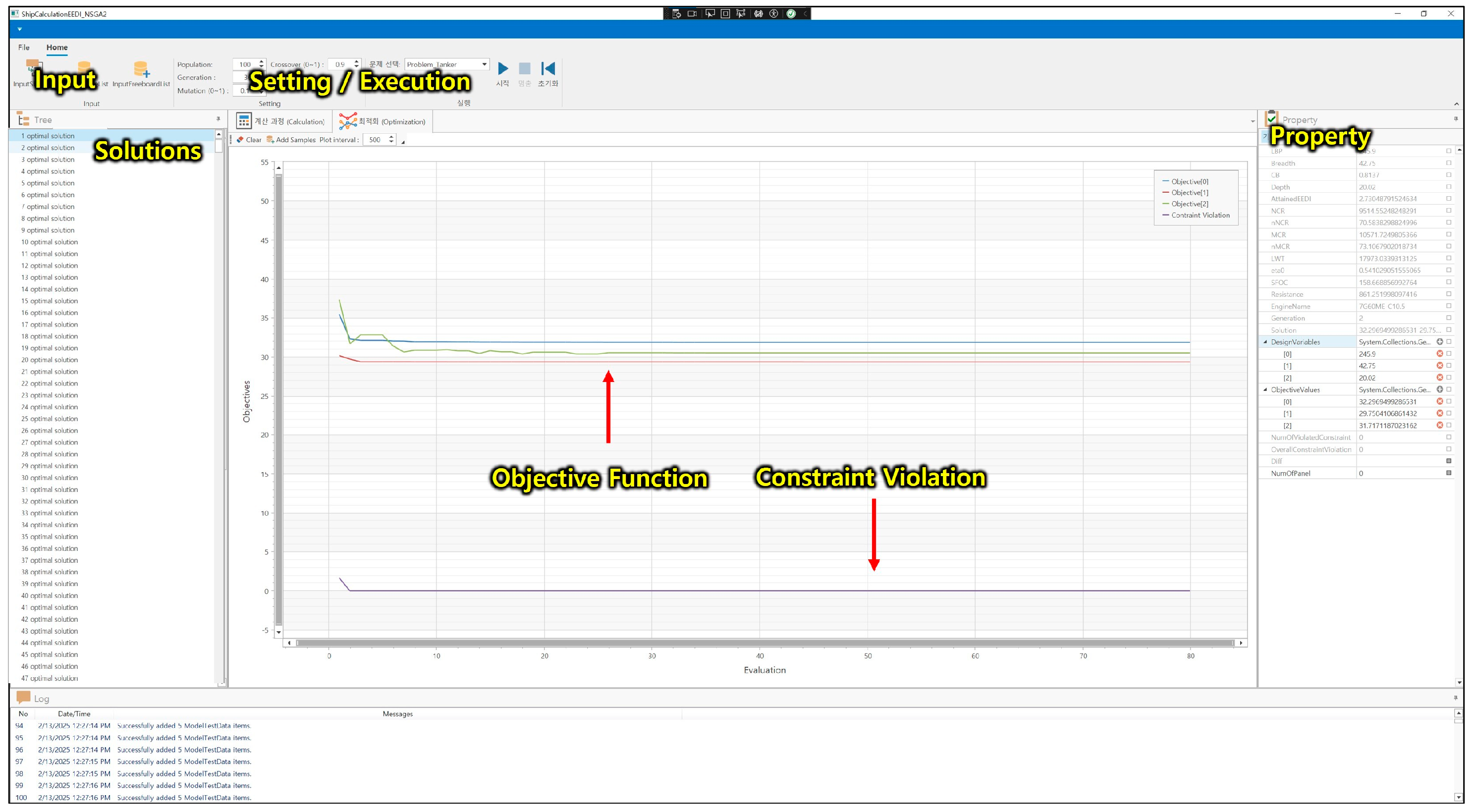
The program developed in this study is shown in Figure 5. Developed using C# and WPF, the program allows the user to monitor the optimization progress and to review the optimal principal dimensions, main engine information, and Attained EEDI corresponding to the optimal solution.

4.2. Optimization Results for 114K Aframax Tanker

In this study, optimization was performed for a 114K Aframax Tanker with VLSFO/LNG dual-fuel capability, satisfying EEDI regulations while considering economic feasibility and operational efficiency. The basis ship particulars are presented in

Table 8. Basis ship information and ship owner’s requirements.

Item	Basis Ship
LOA (m)	Max. 250
LBP (m)	239
Breadth (m)	43.8
Depth (m)	21.0
Design Draft (m)	13.6
Scantling Draft (m)	14.9
Deadweight (ton)	114,800
Speed (knot)	15.0 kts
Main Engine	MAN 6S60MC-C
MCR	18,420 BHP × 105.0 rpm
NCR	16,580 BHP × 101.4 rpm
HFO (m3)	3000
MDO or MGO (m3)	250
Fresh Water (m3)	400
Ballast Water (m3)	40,000
Complement	30 persons
Cargo Tank Capacity (m3)	130,000

.

Based on the weight combinations defined in Table 6. The optimization was conducted with four cases by varying the weight combination assigned to the objective functions—total resistance, SFOC, and LWT. Case 1 is a balanced optimization case in which equal weights (1:1:1) are assigned to all objective functions. Case 2 prioritizes propulsion performance improvement by assigning a higher weight to total resistance. Case 3 aims to minimize SFOC by assigning a higher weight to SFOC. Case 4 prioritizes minimization of shipbuilding cost through steel weight reduction by assigning a higher weight to LWT. The optimization results for each case are presented in

Table 9. Optimization results for 114K Aframax Tanker.

Item	Design Ship	Case 1 (Equal)	Case 2 (Min RT)	Case 3 (Min SFOC)	Case 4 (Min LWT)
LBP (m)	239	242.03	243.27	243.27	238.22
Breadth (m)	43.8	41.96	41.74	42.06	42.85
Depth (m)	21.2	19.61	19.47	21.14	19.57
CB	0.8134	0.8373	0.8376	0.8346	0.8319
RT (kN)	855.1	850.35	849.5	853.93	852.7
SFOC (g/kWh)	166.95	158.36	158.73	158.16	158.23
LWT (ton)	17,904.6	17,280.8	17,451.5	17,776.6	17,128.4
MCR (kW)	10,724 kW × 77.5 rpm	10,678 kW × 73.5 rpm	10,673 kW × 73.5 rpm	10,748 kW × 73.7 rpm	10,762.2 kW × 73.9 rpm
NCR (kW)	9651 kW × 74.8 rpm	9610 kW × 70.9 rpm	9606 kW × 70.8 rpm	9674 kW × 71.7 rpm	9686 kW × 71.36 rpm
Main Engine	MAN 6G60ME-C10.5	MAN 7G60ME-C10.5	MAN 7G60ME-C10.5	MAN 7G60ME-C10.5	MAN 7G60ME-C10.5
η0	0.5245	0.5385	0.5380	0.5411	0.5311
Required EEDI	2.901
Attained EEDI	2.78	2.75	2.76	2.749	2.753

.

All cases satisfied the EEDI Phase 3 standard, and the principal dimensions and performance indicators corresponding to each weight setting were derived. Case 1, as the baseline for balanced optimization, showed reductions of approximately 4.75 kN in total resistance, 8.59 g/kWh in SFOC, and 623.8 tonnes in LWT relative to the design ship. In Case 2, focusing on resistance reduction, the total resistance decreased by approximately 5.6 kN—the largest reduction among all cases—and the required power was accordingly the lowest. This indicates that the principal dimension combination that focused on resistance minimization led to improved propulsive efficiency. In Case 3, the SFOC reduction was the largest at 8.79 g/kWh; however, since the same engine was selected as in the other cases, the absolute difference in SFOC was small. In contrast, total resistance increased by approximately 1.17 kN relative to the design ship, and the LWT reduction was only 128 tonnes—the smallest among all cases—confirming that a weight setting focused on SFOC is unfavorable in terms of resistance performance and steel weight. In Case 4, the LWT reduction was 776.2 tonnes—the largest among all cases—and the principal dimensions were also the smallest, clearly demonstrating the correlation between steel weight reduction and the minimization of principal dimensions.

5. Conclusions

In this study, an optimal principal dimension determination system was developed to maximize the economic feasibility and operational efficiency of a ship while complying with the international maritime regulation of EEDI Phase 3. The developed program automates the iterative and complex calculation process occurring at the early ship design stage through a total of eight Calculation Modules, including LWT Estimation, Resistance Calculation, Main Engine Calculation, and Main Engine Selection. With ${\mathrm{L}}_{\mathrm{B}\mathrm{P}}$, Breadth, Depth, and ${\mathrm{C}}_{\mathrm{B}}$ defined as design variables, a multi-objective optimization was performed using the NSGA-II algorithm to minimize ${\mathrm{R}}_{\mathrm{T}}$, SFOC, and LWT. Application of the developed program to a 114K Aframax Tanker demonstrated reductions of approximately 5 kN in total resistance, 8.59 g/kWh in SFOC, and 623.8 tonnes in LWT relative to the design ship, confirming that both economic feasibility and operational efficiency are simultaneously improved while satisfying EEDI Phase 3. Future work will include extending the application of the proposed methodology to various ship types beyond tankers, such as bulk carriers and container ships, and introducing an economic index considering actual shipbuilding costs to supplement the objective functions.

References

1. Psaraftis, H.N. Shipping Decarbonization in the Aftermath of MEPC 76. Clean. Logist. Supply Chain. 2021, 1, 100008. [Google Scholar] [CrossRef]
2. Trivyza, N.L.; Rentizelas, A.; Theotokatos, G.; Boulougouris, E. Decision Support Methods for Sustainable Ship Energy Systems: A State-of-the-Art Review. Energy 2022, 239, 122288. [Google Scholar] [CrossRef]
3. IMO. Guidelines on the Method of Calculation of the Attained Energy Efficiency Design Index (EEDI) for New Ships (MEPC.1/Circ.795); IMO: London, UK, 2012. [Google Scholar]
4. IMO. Amendments to the Annex of the Protocol of 1997 to Amend MARPOL (MEPC.308(73)); IMO: London, UK, 2018. [Google Scholar]
5. Chen, J.; Xu, J.; You, G.; Li, X. Ship Hull Principal Dimensions Optimization Employing Fuzzy Decision-Making Theory. Math. Probl. Eng. 2016, 2016, 5262160. [Google Scholar] [CrossRef]
6. Park, C. A Study on the Ship Optimal Design Using Hull Form Variation. J. Korean Soc. Mech. Technol. 2018, 20, 238–245. [Google Scholar] [CrossRef]
7. Park, D.-W.; Kim, I. A Study on the Optimization of Main Dimensions of a Ship by Design Search Techniques Based on the AI. J. Korean Soc. Mar. Environ. Saf. 2022, 28, 1231–1237. [Google Scholar] [CrossRef]
8. Wang, H.; Hou, Y.; Xiong, Y.; Liang, X. Research on Multi-Interval Coupling Optimization of Ship Main Dimensions for Minimum EEDI. Ocean Eng. 2021, 237, 109588. [Google Scholar] [CrossRef]
9. Xie, J.; Wang, L.Z.; Wang, H.; Zheng, L. Optimization Design of Ship Main Dimensions with Diffusion Algorithm Based on P Systems. In Proceedings of the ISOPE International Ocean and Polar Engineering Conference; OnePetro: Richardson, TX, USA, 2022; p. ISOPE–I. [Google Scholar]
10. Grigoropoulos, G.J.; Bakirtzoglou, C.; Papadakis, G.; Ntouras, D. Mixed-Fidelity Design Optimization of Hull Form Using CFD and Potential Flow Solvers. J. Mar. Sci. Eng. 2021, 9, 1234. [Google Scholar] [CrossRef]
11. Park, S.-W.; Kim, S.-H.; Kim, Y.-I.; Lee, I. Hull Form Optimization Study Based on Multiple Parametric Modification Curves and Free Surface Reynolds-Averaged Navier–Stokes (RANS) Solver. Appl. Sci. 2022, 12, 2428. [Google Scholar] [CrossRef]
12. Seo, J.; Kim, D.; Lee, I. A Study on Ship Hull Form Transformation Using Convolutional Autoencoder. J. Comput. Des. Eng. 2023, 11, 34–48. [Google Scholar] [CrossRef]
13. Kim, B.-S.; Oh, M.-J.; Lee, J.-H.; Kim, Y.-H.; Roh, M.-I. Study on Hull Optimization Process Considering Operational Efficiency in Waves. Processes 2021, 9, 898. [Google Scholar] [CrossRef]
14. Kim, K.-S.; Roh, M.-I. Review of Ship Arrangement Design Using Optimization Methods. J. Comput. Des. Eng. 2024, 12, 100–121. [Google Scholar] [CrossRef]
15. Jung, S.-K.; Roh, M.-I.; Kim, K.-S. Arrangement Method of a Naval Surface Ship Considering Stability, Operability, and Survivability. Ocean Eng. 2018, 152, 316–333. [Google Scholar] [CrossRef]
16. Yurdakul, O.; Küçüksu, G.N.; Saydam, A.Z.; Çalşal, M.S. A Decision-Making Process for the Selection of Better Ship Main Dimensions by a Pareto Frontier Solution. Ocean Eng. 2021, 239, 109908. [Google Scholar] [CrossRef]
17. Deng, R.; Wang, S.; Hu, Y.; Wang, Y.; Wu, T. The Effect of Hull Form Parameters on the Hydrodynamic Performance of a Bulk Carrier. J. Mar. Sci. Eng. 2021, 9, 373. [Google Scholar] [CrossRef]
18. Lee, S.-M.; Lee, J.H.; Roh, M.-I.; Kim, K.-S.; Ham, S.-H.; Lee, H.-W. An Optimization Model of Tugboat Operation for Conveying a Large Surface Vessel. J. Comput. Des. Eng. 2021, 8, 654–675. [Google Scholar] [CrossRef]
19. de Winter, R.; van Stein, B.; Dijkman, M.; Bäck, T. Designing Ships Using Constrained Multi-Objective Efficient Global Optimization. In Machine Learning, Optimization, and Data Science; Springer: Cham, Switzerland, 2019; pp. 191–203. [Google Scholar]
20. Ha, J.; Roh, M.-I.; Ham, S.-H.; Lee, S.-J. Optimum Design of the Underwater Discharge System Based on Surrogate Modeling. J. Mar. Sci. Technol. 2021, 29, 346–362. [Google Scholar] [CrossRef]
21. Kim, M.; Ham, S. Planning Optimal Refloating Plan to Minimize Ground Reaction Force and Refloating Cost. J. Ocean Eng. Technol. 2025, 39, 489–502. [Google Scholar] [CrossRef]
22. Kim, J.-H.; Roh, M.-I.; Yeo, I.-C. A Method for Generating Multiple Hull Forms at Once Using MLP (Multi-Layer Perceptron). Ocean Eng. 2025, 324, 120659. [Google Scholar] [CrossRef]
23. Tadros, M.; Ventura, M.; Guedes Soares, C. Review of the Decision Support Methods Used in Optimizing Ship Hulls towards Improving Energy Efficiency. J. Mar. Sci. Eng. 2023, 11, 835. [Google Scholar] [CrossRef]
24. Papanikolaou, A. Ship Design; Springer: Dordrecht, The Netherlands, 2014; ISBN 978-94-017-8750-5. [Google Scholar]
25. Kim, J.-H.; Roh, M.-I.; Yeo, I.-C. Hull Form Optimization of Fully Parameterized Small Ships Using Characteristic Curves and Deep Neural Networks. Int. J. Nav. Archit. Ocean Eng. 2024, 16, 100596. [Google Scholar] [CrossRef]
26. Nikolopoulos, L.; Boulougouris, E. A Study on the Statistical Calibration of the Holtrop and Mennen Approximate Power Prediction Method for Full Hull Form, Low Froude Number Vessels. J. Ship Prod. Des. 2019, 35, 41–68. [Google Scholar] [CrossRef]
27. Roh, M.I.; Lee, K.Y. Computational Ship Design; Springer: Singapore, 2017; pp. 1–353. [Google Scholar] [CrossRef]
28. Holtrop, J.; Mennen, G.G.J. An Approximate Power Prediction Method. Int. Shipbuild. Prog. 1982, 29, 166–170. [Google Scholar] [CrossRef]
29. Holtrop, J. A Statistical Re-Analysis of Resistance and Propulsion Data. Int. Shipbuild. Prog. 1984, 31, 272–276. [Google Scholar]
30. Keller, J. Enige Aspecten Bij Het Antwerpen Van Scheepsschroeven. Schpen Werf 1966, 24, 658–663. [Google Scholar]
31. Burrill, L.C.; Emerson, A. Propeller Cavitation: Further Tests on 16in. Propeller Models in the King’s College Cavitation Tunnel1. Int. Shipbuild. Prog. 1963, 10, 119–131. [Google Scholar] [CrossRef]
32. Deb, K.; Pratap, A.; Agarwal, S.; Meyarivan, T. A Fast and Elitist Multiobjective Genetic Algorithm: NSGA-II. IEEE Trans. Evol. Comput. 2002, 6, 182–197. [Google Scholar] [CrossRef]
Figure 1. Impact of principal dimensions on cost, propulsion performance, and regulatory compliance.
Jmse 14 00939 g001
Figure 2. Iterative calculation procedure for determining ship principal dimensions.
Jmse 14 00939 g002
Figure 3. System configuration for determination of optimal principal ship dimensions considering EEDI and operational efficiency.
Jmse 14 00939 g003
Figure 4. SFOC values by engine load for different engines.
Jmse 14 00939 g004
Figure 5. Application optimization interface.
Jmse 14 00939 g005