Article

Elastic Lithospheric Thickness and Its Controlling Factors in the Dual-Subduction System of Taiwan


1
Institute of Earthquake Research, China Earthquake Administration, Wuhan 430071, China
2
Key Laboratory of Earthquake Geodesy, China Earthquake Administration, Wuhan 430071, China
3
Hubei Earthquake Administration, Wuhan 430071, China
*
Author to whom correspondence should be addressed.
J. Mar. Sci. Eng. 2026, 14(10), 911; https://doi.org/10.3390/jmse14100911
Submission received: 22 April 2026 / Revised: 9 May 2026 / Accepted: 11 May 2026 / Published: 14 May 2026
(This article belongs to the Special Issue Bathymetry and Seafloor Mapping)

Abstract

The tectonic setting of Taiwan and its surrounding regions is characterized by the complex interaction between the northwest-oriented Ryukyu subduction zone and the east-oriented Manila subduction zone. Within this subduction framework, the elastic thickness of the lithosphere (Te) serves as a critical parameter for elucidating the mechanical behavior of the area. In this study, we employed the admittance–correlation method to estimate Te values across Taiwan and adjacent territories. The findings indicate that sedimentary loading results in an overestimation of the maximum Te by approximately 50 km; after adjustment, the Te values range from 0 to 60 km throughout the study area. On Taiwan, Te values predominantly lie between 20 and 30 km, decreasing to 10–20 km near the margins adjacent to the Ryukyu and Manila subduction fronts. The Philippine Sea Plate exhibits comparatively higher Te values, ranging from 40 to 65 km. The spatial distribution of Te broadly corresponds with major tectonic subdivisions. Statistical analyses reveal a weak negative correlation between Te and surface heat flow (r = −0.44) and a weak positive correlation with shear-wave velocity anomalies at a depth of 100 km (r = 0.22), suggesting that the thermal structure exerts only a moderate influence on lithospheric strength in this region. Nonetheless, within oceanic crustal domains, the relationship between Te and oceanic crustal age largely adheres to models of crustal cooling and lithospheric thickening, consistent with isotherm depths of approximately 200–400 °C. Additionally, dynamic topography associated with slab subduction may locally diminish Te by up to 25 km. Cross-sectional profiles through northern Taiwan and the Philippine Sea block reveal pronounced coupling between subduction geometry and Te distribution. The observed spatial patterns of Te reflect the mechanical imprint of prolonged tectonic evolution, with the orientation of Te gradients generally aligned with the direction of maximum principal compressive stress. Collectively, these results suggest that subduction geometry and tectonic processes are important factors influencing the spatial variability and evolutionary trajectory of lithospheric strength in Taiwan and its environs.

1. Introduction

Taiwan and its neighboring regions are situated at the convergence zone of the Eurasian Plate and the Philippine Sea Plate, characterized by active tectonic activity and frequent seismic events. The uplift of Taiwan is primarily driven by arc–continent collision processes [1,2], while the interaction between the Manila and Ryukyu subduction systems, which intersect at a high angle (~90°), further modulates the regional tectonic evolution [3]. The southern Manila subduction zone involves relatively young oceanic lithosphere, which is between 16 and 36 million years old, with its fore-arc area significantly influenced by substantial sediment loading and boundary forces [4]. Conversely, the oceanic lithosphere subducting beneath northern Taiwan from the Ryukyu Trench is older, ranging from 40 to 60 million years in age and possessing a crustal thickness of approximately 6 to 10 km [5]. Notably, slab tearing has been documented beneath northern Taiwan [6]. High-resolution earthquake hypocenter locations and seismic tomography studies have revealed pronounced geometric disparities between these two slabs, including marked variations in dip angles at depth [7,8]. Furthermore, low-velocity and high-attenuation anomalies detected within the Manila–Taiwan–Ryukyu transition zone [9] indicate localized fluid enrichment and a thermally weakened lithosphere. These dynamic processes governed by subduction render Taiwan an exceptional natural laboratory for investigating lithospheric evolution.
The elastic thickness of the lithosphere (Te) serves as a critical parameter indicative of its long-term mechanical strength and is influenced by multiple geodynamic factors. Prior research has demonstrated that the regional thermal structure regulates lithospheric strength by altering temperature distributions and rheological properties [10,11], whereas tectonic processes contribute to large-scale spatial variations in Te [12,13]. Additionally, substantial sedimentary loading can affect gravity–topography coupling, thereby partially obscuring the intrinsic strength of the lithosphere [14,15]. Although there is a consensus that the lithosphere beneath Taiwan is generally weak [16,17,18], significant discrepancies persist regarding the magnitude and spatial distribution of Te across different studies [19,20,21,22,23]. These inconsistencies primarily arise from variations in datasets, inversion methodologies, and the complex tectonic setting. A comprehensive evaluation of the interplay among Te, thermal properties, and tectonic processes within this dual-subduction system remains absent.
To address this gap, we utilize the WGM2012 global gravity model, GEBCO 2025 topographic and bathymetric data, and the CRUST1.0 crustal model, supplemented by sediment corrections based on the GlobSed database, to conduct a joint admittance–coherence inversion aimed at delineating the spatial distribution of Te in Taiwan and its adjacent regions. Subsequently, we examine the correlations between Te and thermal indicators, including surface heat flow and upper-mantle S-wave velocity anomalies, as well as the age of the oceanic lithosphere and the impact of subducting slabs on Te. In particular, this study explores whether lateral heterogeneity in lithospheric mechanical strength, as reflected by Te gradients, may influence the spatial distribution of present-day tectonic stress within the dual-subduction system of Taiwan. These analyses offer novel insights into lithospheric deformation and tectonic dynamics under the dual-subduction regime characteristic of the Taiwan region.

2. Geological Background

Plate convergence between the Eurasian Plate and the Philippine Sea Plate fundamentally governs tectonic processes in the Taiwan region. In the eastern sector, the Philippine Sea Plate descends northwestward beneath the Eurasian margin at 8–9 cm/yr, forming the Ryukyu island-arc and back-arc basin system [24,25]. In southern Taiwan, the Manila subduction zone is defined by the eastward subduction of the South China Sea Plate beneath the Philippine Sea Plate at a rate of roughly 6–8 cm per year, giving rise to the Luzon island arc–Manila Trench system [26]. Situated at the junction of these two significant subduction systems, the Taiwan orogenic belt displays characteristic features of arc–continent collision, with foreland basins and foreland complexes developed on its eastern and western flanks, respectively [27,28]. Additionally, extensive thick sedimentary sequences are present in the regions adjacent to Taiwan, particularly within the western foreland basin and the southern accretionary wedge, where sediment thicknesses reach between 3 and 5 km. These sequences predominantly comprise terrigenous and marine sediments from the Miocene epoch [29,30]. These sedimentary deposits play a critical role in the subduction process and have the potential to introduce biases in thermal (Te) inversion analyses [31].

3. Data and Methods

3.1. Data

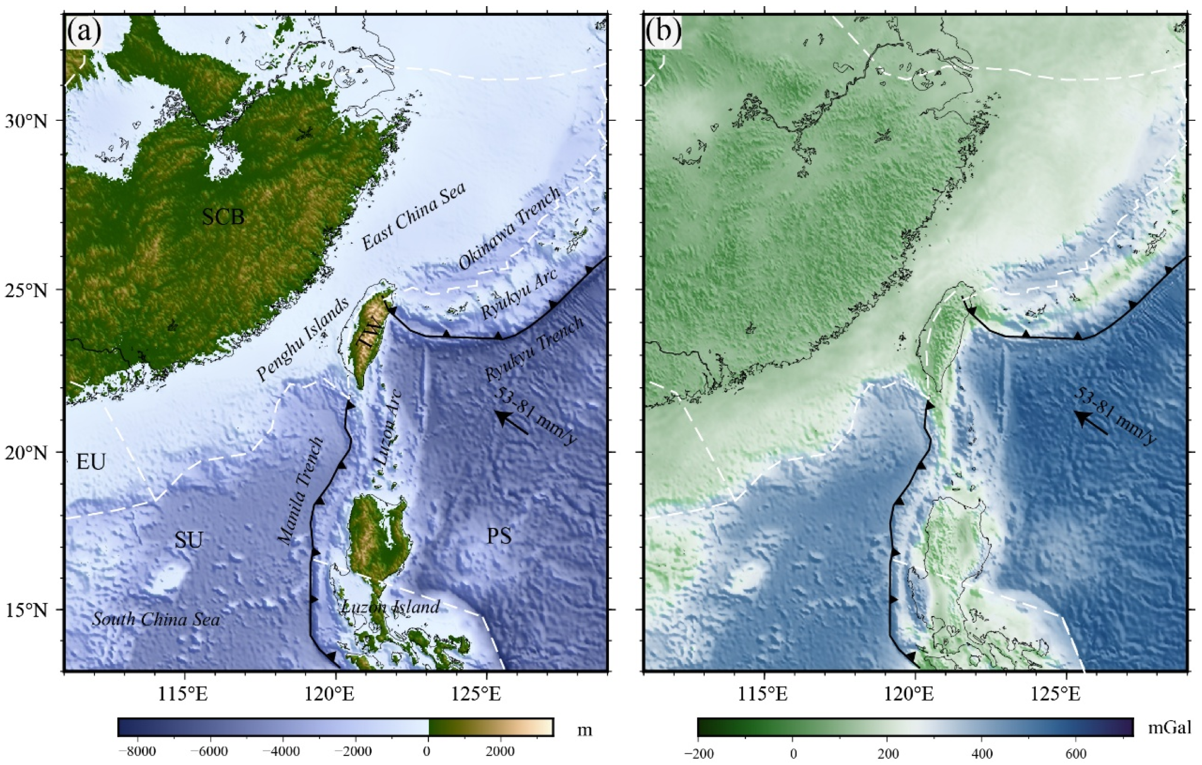
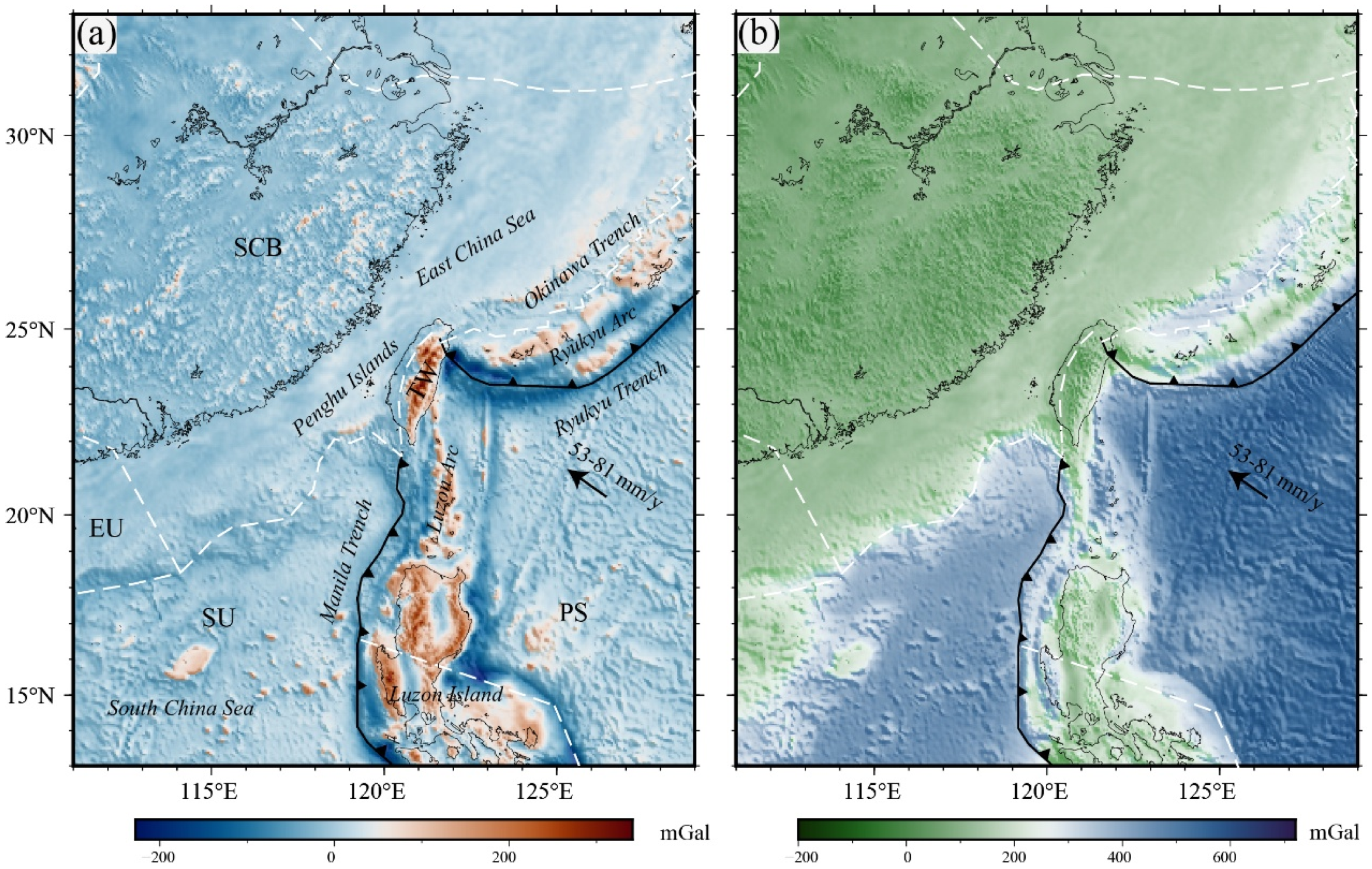
Topographic and bathymetric data were obtained from the GEBCO_2025 global grid (https://www.gebco.net/, accessed on 13 October 2025), which provides near-global coverage of elevation and seafloor depth. Compared to the ETOPO1 model, the GEBCO dataset is primarily constrained by shipboard measurements, thereby reducing dependence on satellite-altimetry-derived gravity information. This improves the independence between topography and gravity data and minimizes the risk of artificial coherence in subsequent spectral analyses. The dataset has a spatial resolution of 15 arc-seconds, allowing for a detailed representation of the terrain and seafloor morphology within the study region (Figure 1). Free-air gravity anomaly data were sourced from the WGM2012 global gravity model [32], which integrates measurements from GRACE satellites, shipborne surveys, and terrestrial gravity observations, with values spanning roughly −200 mGal to 320 mGal (Figure 2a). The dataset has a spatial resolution of 2 arc-minutes. Bouguer and topographic corrections were computed using FA2BOUG FORTRAN 90 software [33], yielding Bouguer gravity perturbations ranging between −200 mGal and 720 mGal (Figure 2b).
The study area encompasses both continental and marine lithospheric domains, with the marine sector subject to the influence of water loading. To harmonize loading conditions across these environments, the methodology proposed by Stark et al. [34] and Kirby and Swain [35] was employed to convert seawater loads into equivalent crustal loads prior to performing Fourier transforms. This conversion is expressed by the formula
h eq = h ( ρ uc ρ w ) / ρ uc
where ρw and ρuc denote the densities of seawater (1030 kg/m3) and the upper crust (2670 kg/m3), respectively. This approach facilitates the application of a unified loading equation across the entire study area, thereby obviating the need for separate computations for terrestrial and marine regions and preventing discontinuities in Te results at the coastline [36,37].

3.2. Sedimentary Layer Correction

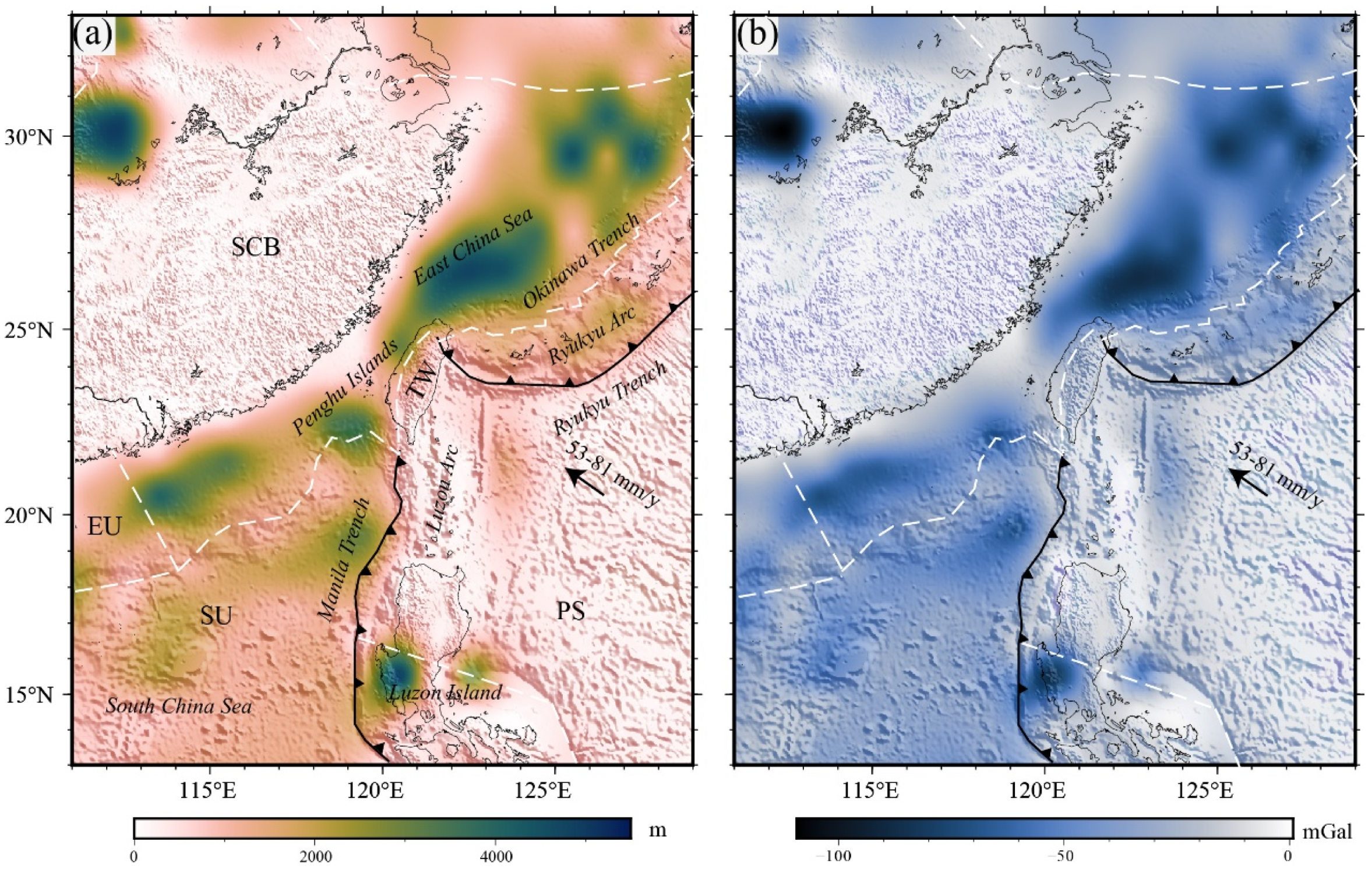
Sedimentary layers exert a significant influence on Te estimations derived from spectral methods, as the density contrast between sediments and the underlying basement rocks can induce substantial gravity anomalies [20,38,39]. The presence of thick sedimentary sequences modifies the correlation between topography and gravity, often resulting in an overestimation of Te if uncorrected. Figure 3a presents sediment thickness data for the study area obtained from the GlobSed model [40] at a spatial resolution of 5 arc-minutes. Sediments are predominantly distributed within the South China Block and the adjacent coastal waters of Eastern China, particularly in the East China Sea, where sediment thickness exceeds 5 km. These sedimentary accumulations can generate gravity anomalies reaching magnitudes of approximately −110 mGal (Figure 3b). To mitigate the effects of sedimentary layers, we applied spherical prism forward modeling [41] for sediment correction. The fundamental principle involves treating the sedimentary layer as an integral component of the Earth’s crust by substituting the sediment with rock of average crustal density and subsequently calculating the resultant modifications in topography and gravity.
h eq = h ( ρ uc ρ w ) / ρ uc + s ( ρ s ρ uc ) / ρ uc
In this context, ρs and s denote the density and thickness of the sedimentary layer as indicated in the respective dataset. For the purpose of facilitating comparison, Figure 4 presents the topographic and Bouguer gravity data subsequent to the removal of the sedimentary layer. This adjustment effectively mitigates the influence of the unexposed subsurface load and substantially decreases the estimated Te in regions characterized by minimal topographic variation and where variations in the density of the sedimentary cover predominate [10,31,41].

3.3. Dynamic Topographic Calculation of Subducting Blocks

The dual-subduction system within the study region exerts a considerable influence on the calculation of Te. The perturbations in topography and gravity induced by subduction processes are dynamic topographic and gravity anomalies, which function as noise signals in the estimation of Te [42]. Following the methodology developed by Husson [43], the tension (Fj) exerted by a subducting plate element i at a surface observation point j can be quantified using Equation (3):
F j = 3 Δ ρ ν i g z i 3 π r i j 5
Here, Δρ denotes the density contrast between the subducting plate element and the mantle; vi and zi represent the unit volume and depth of the plate element, respectively; g is the acceleration due to gravity; and rij is the distance separating the plate element from the observation point. This tension Fj induces lithospheric deflection, resulting in surface deflection hij. The aggregate surface deflection Hj at the observation point can be computed using Equation (4):
H j = i 3 Δ ρ ν i z i 3 π r i j 5 ( ρ m ρ )
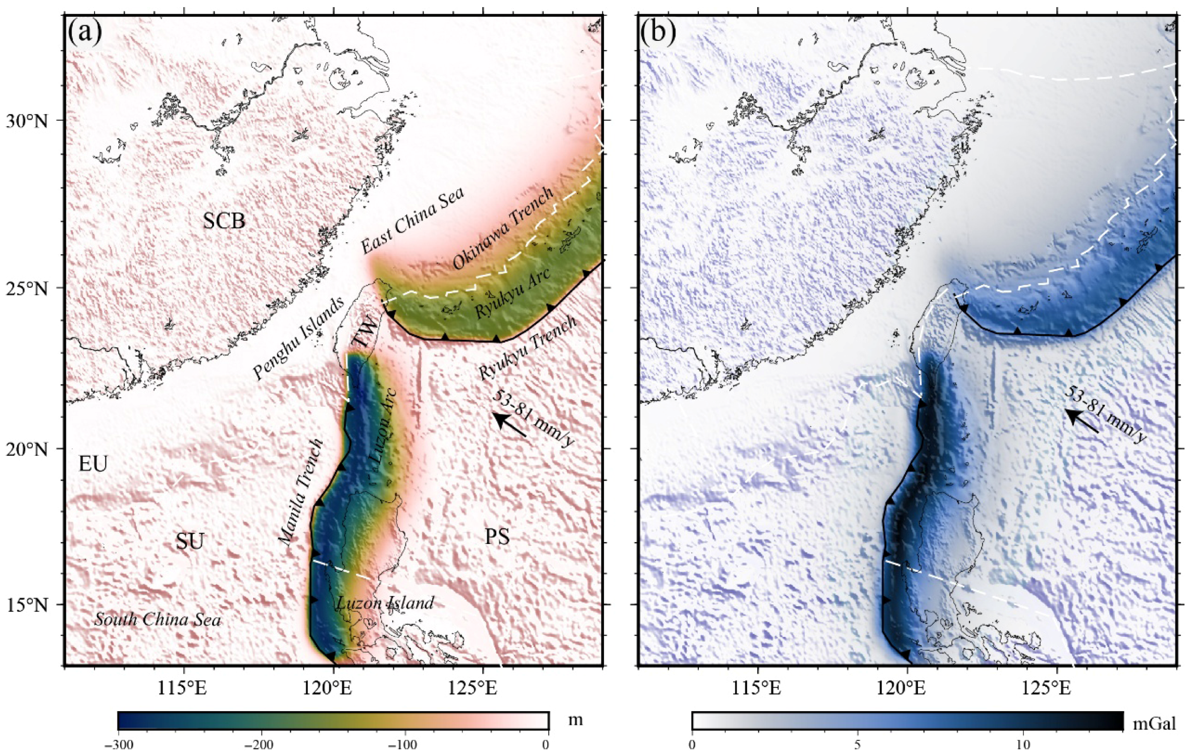
where ρm is the density of the mantle, while ρ* denotes the density of the overlying medium and is assigned according to the geological setting, with air density used for land areas and seawater density used for oceanic regions. The subduction depth data employed in these calculations are sourced from Hayes et al. [44]. The thickness reference for the Manila subduction zone is derived from Eakin et al. [4], with an average thickness of 12 km, whereas for the Ryukyu subduction, typified by oceanic crust subduction, we utilize a thickness reference from Wang et al. [5], averaging 9 km. The resultant dynamic topography and Bouguer gravity disturbances are illustrated in Figure 5. The maximum perturbations in topography and Bouguer gravity anomalies attributable to the Manila and Ryukyu subductions are approximately −300 m and 13 mGal and −160 m and 8 mGal, respectively.

3.4. Method for Calculating Te

The effective elastic thickness (Te) of the lithosphere serves as an indicator of its mechanical strength under geological loading conditions over timescales exceeding 105 years. Its relationship with flexural rigidity (D) is expressed as per Walcott’s approach [45]:
D = E T e 3 12 ( 1 ν 2 )
To estimate Te, we compute the admittance and coherence functions between topographic and Bouguer gravity anomalies [45], fitting these observations to a simplified thin elastic plate model governed by combined surface and subsurface loading [46,47]. The relative contribution of loading is characterized by the average load ratio F = f/(1 + f) at the transition wavenumber [48], where F = 1 (f → ∞) indicates loading entirely from subsurface sources, and F = 0 (f → 0) corresponds to loading exclusively from surface sources. Spectral estimation of admittance and coherence is performed using the sector wavelet transform method [49], which facilitates collection of spatially variable coherence estimates at each grid point. The Morlet wavelet, with a central wavenumber |k0| = 5.336, is employed to prioritize wavenumber resolution [35].
χ 2 ( F , T e ) = 1 ( 2 N 2 ) j = 1 2 i = 1 N d i j S i j ( F , T e ) ε i j 2
where N denotes the number of samples; j = 1 corresponds to admittance and j = 2 to correlation; dij represents the observed admittance or correlation function data values; Sij denotes the predicted values derived from the mechanical response model; and εij signifies the variance between observed and predicted values. Adopting the approach outlined by Forsyth [50], we employ a single-layer crustal model to estimate the crustal structure, wherein internal loading is assumed to act upon the Moho discontinuity. The depth of the Moho and the crustal density parameters were sourced from the CRUST1.0 global crustal model [51], with a spatial resolution of 1° × 1°. To mitigate errors arising from the planar approximation of curved coordinates, all datasets were transformed into a Cartesian coordinate system via the Mercator projection, utilizing a grid spacing of 10 km. Subsequent dataset comparisons and calculations were performed after interpolation to the same spatial resolution. Prior to performing the Fourier transform, we extended the gravity and topographic data by 2 degrees at the boundaries. This extension, in conjunction with the application of a wavelet transform, was found to exert a negligible influence on the results [22]. Subsequently, the optimal values of effective elastic thickness (Te) and loading ratio (F) were determined through nonlinear least squares optimization. The fitting error between the admittance and coherence functions was assessed using a simplified chi-square criterion [52]. The principal parameters utilized in this analysis and reference values are summarized in Table 1.

4. Results

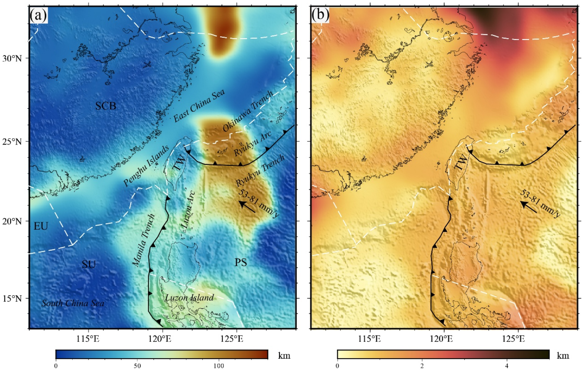
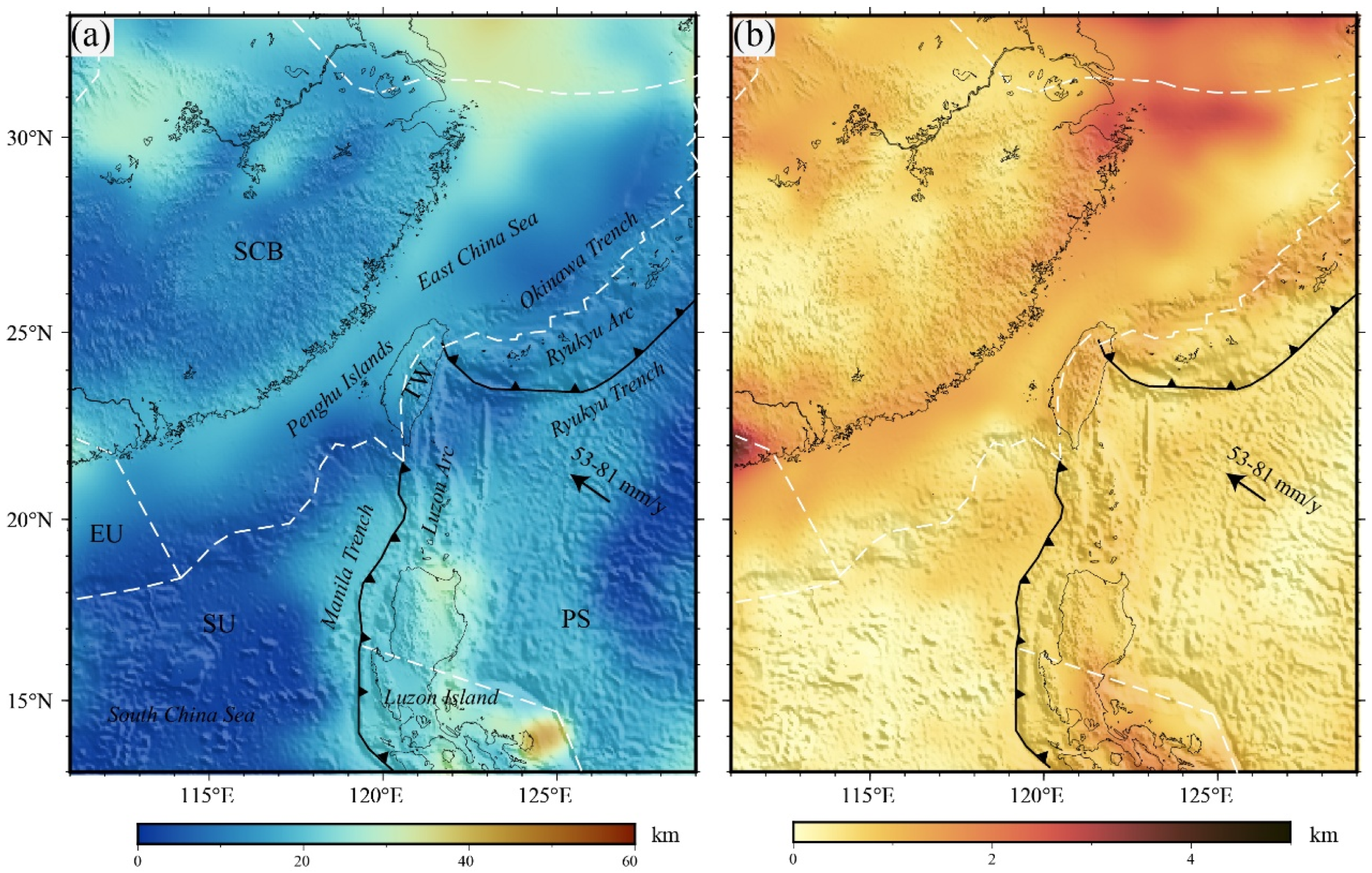
The spatial distributions of both uncorrected and sediment-corrected Te values were obtained, as shown in Figure 6a and Figure 7a. Differences of up to approximately 50 km can be observed, with the largest corrections concentrated in sediment-rich regions, particularly in the northern East China Sea, the Ryukyu Trench, and the Okinawa Trough. Regionally, the sediment correction generally reduces Te estimates by about 20–30 km in the Manila Trench and around Luzon Island, whereas comparatively smaller changes (<5 km) can be observed within the central South China Block and the southern Philippine Sea Plate. This difference indicates that sedimentary correction is essential in the estimation of Te.
In general, the spatial pattern of Te demonstrates pronounced tectonic differentiation. Post-correction, the Te values within the study area range from 0 to 60 km (Figure 7a). The spatial variability in the Te obtained aligns well with findings from previous investigations [19,20], thereby affirming the reliability of the present calculations. Notably, the observed differences are concentrated in tectonically complex regions such as subduction zones, island arcs, and oceanic islands, reflecting heterogeneity in lithospheric mechanical evolution across diverse tectonic settings. Within the South China Block, the Te exhibits a thinner central zone flanked by a thickened periphery, with values of 10–20 km along the continental margin extending toward the East China Sea, consistent with the results reported by Lu [53] and Luo Fan [54]. Significant variations are also evident in Taiwan and its associated subduction zones; the highest Te values (20–30 km) are found in the core of the Central Mountain Range, whereas the eastern margin of the Ryukyu Trench and the southwestern margin of the Manila Trench display Te values ranging from 10 to 20 km. These ranges correspond closely with those documented by Xu and Chen [55] and Liu et al. [56], who reported values of 9–20 km and 5–20 km, respectively. Conversely, in the northern portion of the Sunda Block within the South China Sea, Te values are as low as 5–7 km, which is broadly consistent with the approximately 10 km value reported by Guan [57]. A distinct transition zone between regions of strong and weak Te can be observed along the Manila subduction trench extending toward its rear edge. In contrast, the Philippine Sea Plate generally exhibits higher Te values, ranging from 40 to 60 km, with localized reductions to 0–20 km in the eastern sector. These values exceed earlier estimates of 15–40 km reported by Mao et al. [23], while more recent studies by Lu et al. [53] and Shi et al. [20] similarly indicate elevated Te relative to adjacent regions. Given the low surface heat flow documented in this area [58], we infer that the lithosphere possesses greater mechanical strength compared to surrounding regions. Collectively, these findings suggest that the calculated Te values are robust and reliable.

5. Comparison of Te with Thermal Structure Data

5.1. Te with Surface Heat Flow and Shear Wave Velocity Disturbance

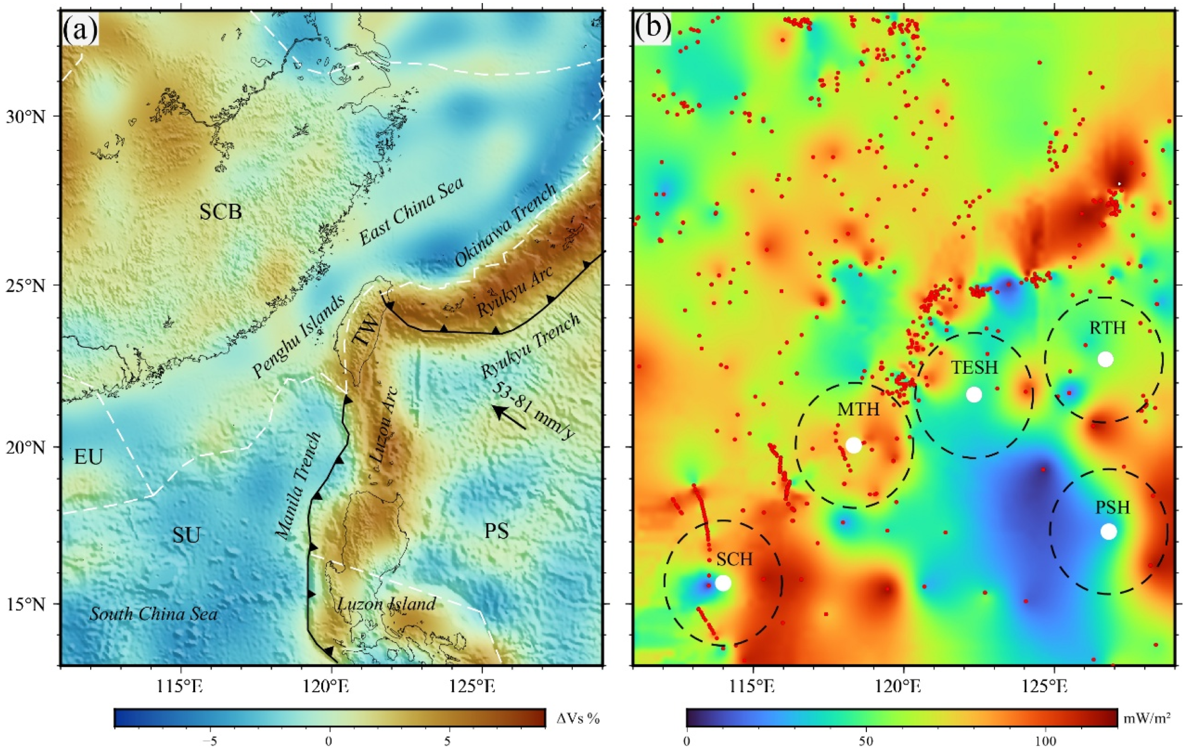
We employ the 0.25° resolution full-waveform tomography data for East Asia, as presented by Liu et al. [59], focusing specifically on the S-wave velocity anomaly (ΔVs) at a depth of 100 km, for comparative analysis. In oceanic domains, particularly for relatively mature oceanic plates, this depth commonly approximates or lies slightly above the lithosphere–asthenosphere boundary. In continental regions, it generally corresponds to the upper portion of the lithospheric mantle beneath relatively thick continental lithosphere. This depth approximates the lithosphere–asthenosphere boundary and is highly responsive to variations in lithospheric thickness, thermal conditions, and fluid activity, thereby serving as a critical stratigraphic level for assessing lithospheric strength heterogeneity. Surface heat flow measurements were sourced from the International Heat Flow Commission (IHFC) global database (http://ihfc-iugg.org/, accessed on 12 December 2025) and supplemented with terrestrial data from China [60], encompassing 1176 observation points. The spatial distribution of heat flow within the study region was derived via Kriging interpolation (Figure 8b). These heat flow data provide direct insights into the shallow thermal regime and energy balance of the lithosphere, offering essential thermal constraints for Te. Utilizing these datasets, we examined the interrelations among Te, ΔVs distribution, and surface heat flow patterns.
The prevailing scholarly consensus is that Te exhibits a negative correlation with the lithospheric thermal state and a positive correlation with ΔVs such that elevated Te values correspond to reduced heat flow [61,62]. This relationship reflects thermo-mechanical coupling, where temperature, composition, and fluid content jointly influence both seismic velocity structure and lithospheric elastic strength, although each proxy responds with different sensitivities. This investigation corroborates this spatial-coupling phenomenon. Within the South China Block, the observed ΔVs anomalies are predominantly of low amplitude, ranging from approximately −3% to 3%, accompanied by modest variations in surface heat flow (50–70 mW/m2), consistent with the presence of laterally heterogeneous high-conductivity layers in the lithosphere. The eastern coastal lithosphere of the South China Block experienced extensional thinning during the Cenozoic epoch [63]. The corresponding Te variations likely reflect the long-term thermo-tectonic modification associated with this extensional regime. The heterogeneous distribution of Te thickness reflects lithospheric weakening associated with this structurally heterogeneous lithosphere [64]. In the northern sector of the Ryukyu subduction zone, Te markedly decreases to approximately 10 km, indicative of pronounced lithospheric attenuation. This reduction aligns with a low S-wave velocity anomaly (−6% to 0%) and elevated heat flow values exceeding 100 mW/m2, suggesting influences from forearc metamorphism and dehydration processes within the subducting slab [65], which collectively contribute to significant lithospheric softening and enhanced susceptibility to bending and fracturing. Conversely, at the leading edge of the Ryukyu subduction zone, S-wave velocities display a high-velocity anomaly, concomitant with an increase in Te. This pattern suggests a colder and mechanically stronger lithospheric state, where reduced thermal perturbation results in higher seismic velocities and increased elastic strength. On the western flank of the Southern Manila subduction zone, a low-velocity slab (Vs ≈ 4.5 km·s−1) is overlain by a low-velocity wedge (Vs = 3.5–3.8 km·s−1); this configuration, coupled with elevated heat flux, corresponds to reduced Te values ranging from 10 to 20 km. The presence of dehydration fluids in this region [66] likely plays a significant role in diminishing lithospheric strength. This interpretation is consistent with a fluid–thermal weakening mechanism, where slab-derived fluids reduce effective viscosity and promote seismic velocity reduction. The Philippine Sea Plate predominantly exhibits a combination of high Te values (50–65 km), low heat flow (30–50 mW/m2), and positive ΔVs anomalies (approximately 3–5%), broadly conforming to the established correlations.
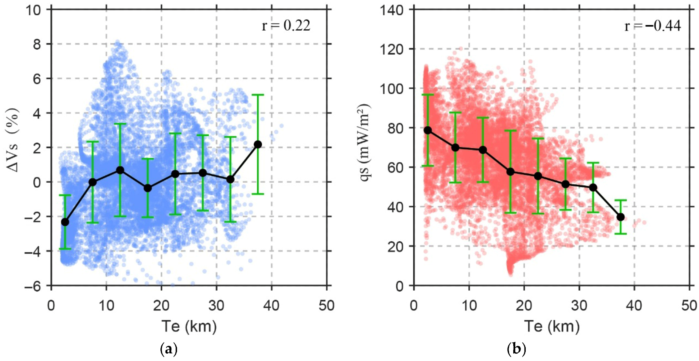
Statistical correlation analysis (Figure 9) revealed that the effective elastic thickness (Te) has a moderate negative correlation with surface heat flow, with a correlation coefficient of r = −0.44. In contrast, its correlation with S-wave velocity anomalies at a depth of 100 km is weakly positive (r = 0.22), aligning with prior findings reported for Southeast Asia [10]. Regions characterized by elevated surface heat flow typically indicate lithospheric heating and consequent weakening, accounting for the pronounced negative correlation observed with Te. Conversely, the S-wave velocity anomaly at a depth of 100 km is governed by factors such as upper-mantle temperature, compositional variations, and fluid presence, whose influences tend to be indirect and spatially localized. Consequently, although the thermal structure exerts an overall influence on Te, the correlation between Te and S-wave velocity anomalies remains comparatively weak.

5.2. Comparison of Te with Oceanic Crust Age

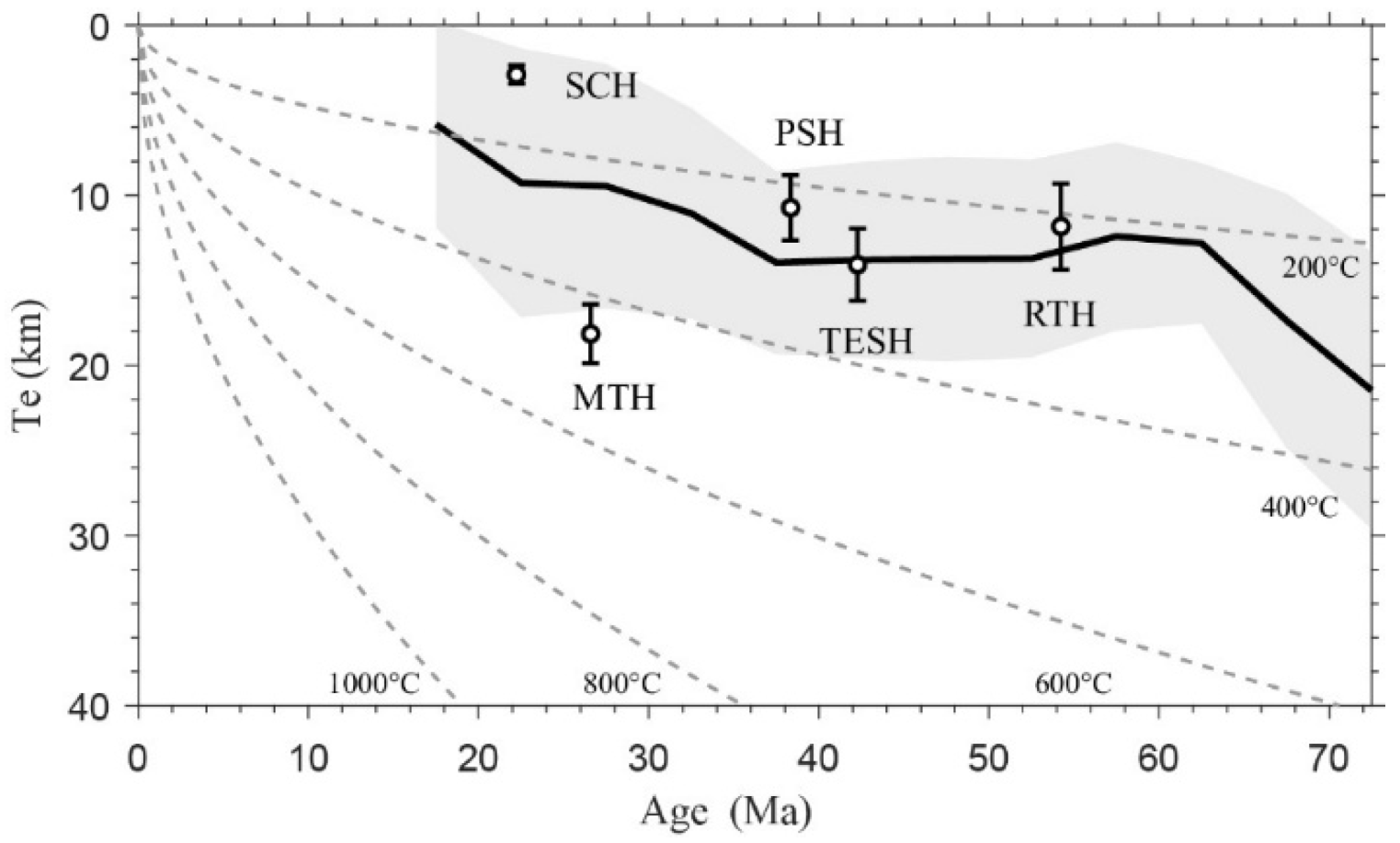
This study examines the relationship between Te and the thermal structure across the investigated region. In oceanic settings, Te is strongly correlated with the age of the oceanic crust and the depths of specific isotherms. Typically, Te corresponds reliably to the depth range of the 300–600 °C isotherm [62] and demonstrates a systematic increase with oceanic crust age, consistent with the classical lithospheric cooling and thickening model [67]. As illustrated in Figure 9, the calculated mean trends for the study area generally align with this model, with the majority of Te values falling within the 200–400 °C isotherm depth interval.
A comparison of oceanic crust ages within a two-degree radius of heat flow measurement points in regions exhibiting inverted Te values reveals distinct patterns, which are summarized in Figure 9. At the TESH, RTH, and PSH sites, oceanic crust ages range from 35 to 60 million years, with corresponding Te values between 10 and 20 km. These values are consistent with the 200–400 °C isotherm depths (Figure 10) and broadly conform to the classical lithospheric cooling–thickening framework [67]. Conversely, at SCH, the oceanic crust is younger than 27 million years, corresponding to lower Te values in the 0–10 km range. Notably, at MTH, the oceanic crust, which is 20–30 million years old, exhibits substantially elevated Te values of 40–45 km, which exceed the 15–20 km thickness predicted by the classical model for crust of a comparable age. These points are situated between the 400 and 600 °C isotherms. Such regional anomalies have also been documented in various subduction zones and hotspot regions globally. For example, in the Canary Islands, Te is associated with isotherms near 650 °C, a phenomenon interpreted as indicative of significant mantle convection beneath the lithosphere [39,68]. Overall, the relationship between crustal age and Te in Taiwan and its adjacent areas aligns with global trends, although deviations observed in certain localities may be attributed to the relatively young age of the oceanic crust. In contrast, older lithospheric regions tend to exhibit a more gradual stabilization of Te consistent with progressive cooling.

6. Tectonic Response to Te

6.1. Influence of Subducting Blocks on Te

Based on the sediment-corrected Te results, the influence of dynamic topography associated with subducting slabs on lithospheric strength is further evaluated. Figure 5, Figure 6b and Figure 11b show the Te estimation errors for the corresponding regions. The Te estimation errors are generally less than 3 km but reach 3–5 km in the northern South China Block and part of the Eurasian Plate. A comparison between Figure 7a and Figure 11a shows that slab-induced dynamic topography generally reduces the effective elastic thickness, with minimum Te values reaching approximately 20 km, while the overall spatial distribution pattern of Te remains broadly consistent before and after correction. Uncertainties associated with assumed slab thicknesses and density contrasts primarily affect the amplitude of the dynamic-topography correction, whereas the spatial characteristics and regional trends of the corrected Te distribution remain relatively stable. The most significant reductions are concentrated in the outer-rise regions of the Ryukyu and Manila subduction systems, particularly around Luzon Island and the Okinawa Trough. In contrast, with increasing distance from the subducting slabs, the magnitude of Te variation gradually decreases from approximately 10 km within the Philippine Sea Plate and the South China Sea Block. This reduction can primarily be observed in the outer uplift regions of the subduction zone and along the boundary between the Sumatra and Philippine Blocks.
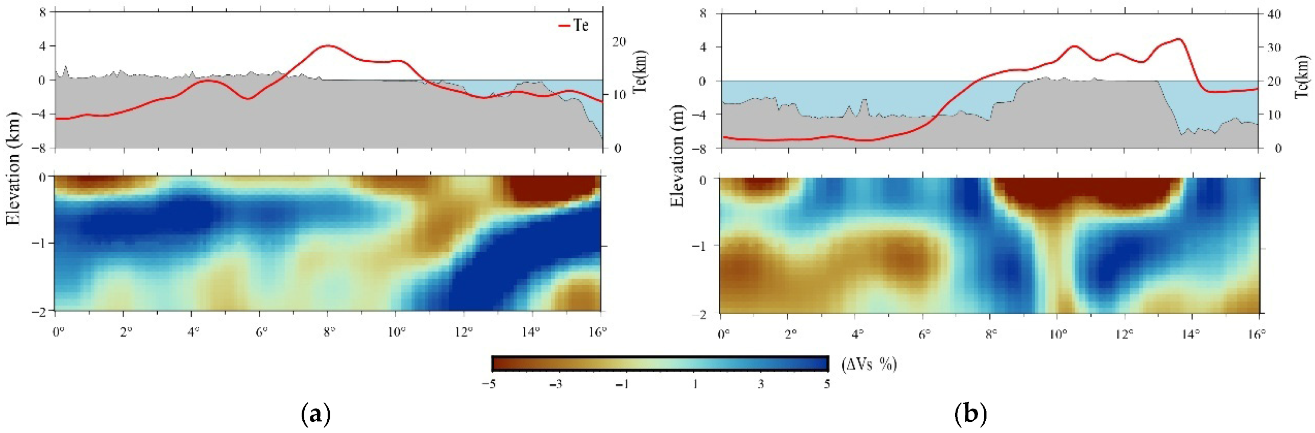
Two representative cross-sectional profiles derived from Figure 11, traversing the northern Taiwan and Philippine Sea blocks, respectively, were analyzed in conjunction with S-wave velocity anomaly distributions at depths ranging from 0 to 200 km. These profiles elucidate the regulatory role of the dual-subduction system on lithospheric strength and structural configuration.
Figure 12b presents a transverse profile across the Philippine Sea block. The western segment of this profile corresponds to the Manila subduction system, where the relatively young and thermally immature Sunda plate subducts eastward at a steep angle, resulting in generally low Te values indicative of a weakened oceanic lithosphere [62]. Progressing eastward through the central Philippine Sea block, an increase in Te can be observed, corresponding to the transition zone from island arc to continental margin, where lithospheric strength is comparatively enhanced. At the easternmost extent of the profile, within the Philippine subduction system characterized by pronounced slab bending, Te values decrease. Along the subduction zone, localized regions of elevated Te are frequently detected; although minor uncertainties in inversion techniques or loading geometry may influence precise measurements, these elevated values reflect authentic lithospheric strengthening attributable to prolonged tectonic processes [19,20]. Extensive research has demonstrated that subduction processes systematically alter the mechanical structure of the lithosphere. For instance, elevated Te values observed at the Zealandia subduction zone are interpreted as evidence of lithospheric reinforcement resulting from subduction interface interactions [70]. Similarly, abrupt variations in Te across the Tibetan Plateau correspond to the subduction of the rigid Indian lithospheric slab [53]. In the northern Taiwan profile (Figure 12a), Te exhibits significant spatial variability: the central segment aligns with the Taiwan orogenic belt, where maximum Te values coincide with lithospheric thickening and strengthening induced by sustained convergent compression. Conversely, the eastern segment corresponds to the Ryukyu subduction system, characterized by a concave slab geometry and a relatively shallow subduction angle, accompanied by a gradual decline in Te values. Collectively, these observations show that the spatial distribution of Te in Taiwan and adjacent regions is intimately associated with subduction slab geometry, highlighting the predominant influence of subduction structures on the large-scale mechanical strength of the lithosphere. Notably, elasto-plastic flexural modeling can better constrain the lithospheric mechanical structure but requires additional assumptions. Future integration with flexural modeling may further refine these interpretations.

6.2. Comparison of Te Gradient and Principal Stress Direction

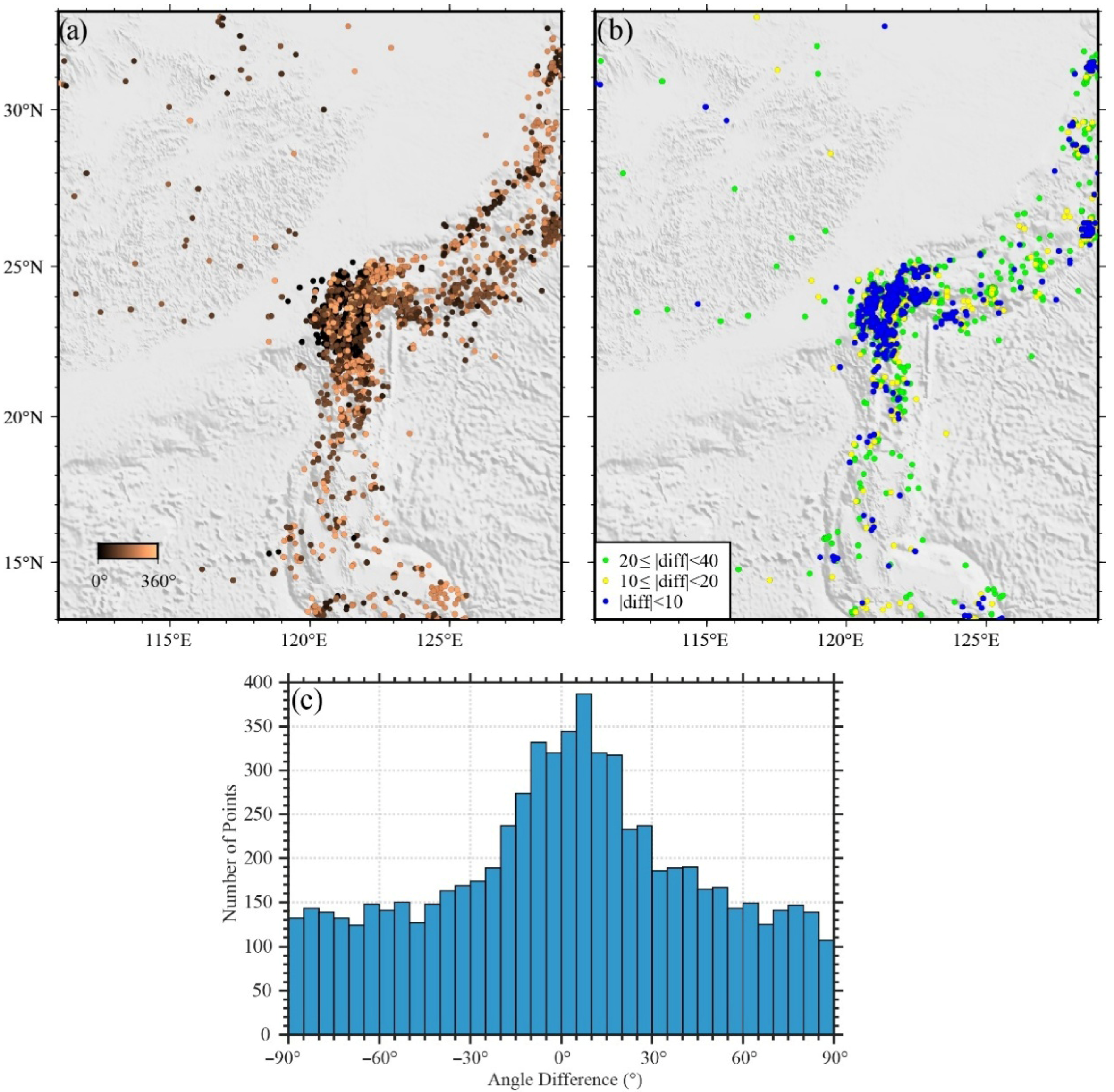
As delineated in the preceding section, large-scale tectonic processes governed predominantly by the subduction system exert a substantial influence on the spatial distribution of lithospheric strength. The gradient of Te serves as an indicator of the principal direction of variation in lithospheric rigidity, while S1 denotes the orientation of the maximum principal compressive stress within the current tectonic regime. To further investigate the coupling between the long-term lithospheric strength configuration and the contemporary stress field, we undertook a comparative analysis between the horizontal gradient of the Te field and the S1 orientation derived from the World Stress Map (WSM, www.world-stress-map.org, accessed on 12 December 2025).
A dataset comprising 6928 stress measurement points within the Taiwan–Luzon tectonic domain was analyzed. Statistical evaluation revealed that approximately 20% of these points exhibit an angular discrepancy |Δθ| ≤ 10°, 36.5% fall within 20°, and 58.8% fall within 40°, indicating a moderate degree of directional concordance in specific regions (Figure 13). These results corroborate prior findings concerning the association between Te and zones of pronounced tectonic activity [18,71,72]. Spatially, areas characterized by minimal Te gradients are predominantly located within the Taiwan Orogenic Belt, which is typified by low Te values and intense crustal deformation. Conversely, along the northern margins of the Ryukyu and Manila subduction zones, the angular difference between the Te gradient and S1 azimuth generally ranges from 20° to 40° (Figure 13). This region is marked by oblique convergence coupled with right-lateral strike-slip motion between the Eurasian Plate and the Philippine Sea Plate [73], manifesting rotational characteristics within the tectonic stress field. The complex interplay of strain regimes in this area engenders a divergence between the direction of lithospheric strength variation and the prevailing principal compressive stress orientation. Previous investigations [74] have posited that mantle-driven stresses may exert a significant influence in regions where the lithosphere exhibits resistance to deformation, as reflected by higher Te values. This hypothesis aligns with observations in southern Taiwan and the Philippine Sea blocks, suggesting that the observed misalignment between lithospheric strength distribution and stress orientation within the strike-slip–subduction transition zone may reflect the combined effects of mantle flow dynamics and plate interactions.
It is imperative to underscore that the Te gradient does not intrinsically represent a stress direction, and its physical interpretation is not directly analogous to that of S1. Consequently, the comparative analysis is not intended to establish a direct mechanical equivalence but rather to evaluate the extent to which the long-term lithospheric strength architecture modulates present-day tectonic strain. Specifically, the Te gradient encapsulates the spatial heterogeneity of lithospheric stiffness, preserving the long-term stratification and tectonic vestiges resultant from subduction system evolution, whereas the stress field embodies the dominant mechanisms governing active tectonics at present. This distinction elucidates why perfect correspondence between these parameters is not anticipated.

7. Conclusions

In this research, we employed the admittance–correlation method, incorporating corrections for sedimentary layers and subduction blocks, to estimate the effective elastic thickness (Te) distribution across Taiwan and its adjacent regions. We systematically investigated the relationships between Te and several geophysical parameters, including the S-wave velocity anomaly at a depth of 100 km, surface heat flow, oceanic crust age, and tectonic characteristics. The principal findings are summarized as follows.
The Te values within the study area range from 0 to 65 km. The South China Block displays a characteristic “thin-middle, thick-periphery” pattern. In Taiwan, Te locally increases to 20–30 km but decreases to 10–20 km near the subduction fronts at both extremities. The Philippine Sea Plate exhibits relatively high Te values overall (30–60 km), with the continental segment maintaining stability between 40 and 60 km. Notable thinning of Te occurs in the northern South China Sea and along the eastern margin of the South China Block, where the minimum values fall below 10 km.
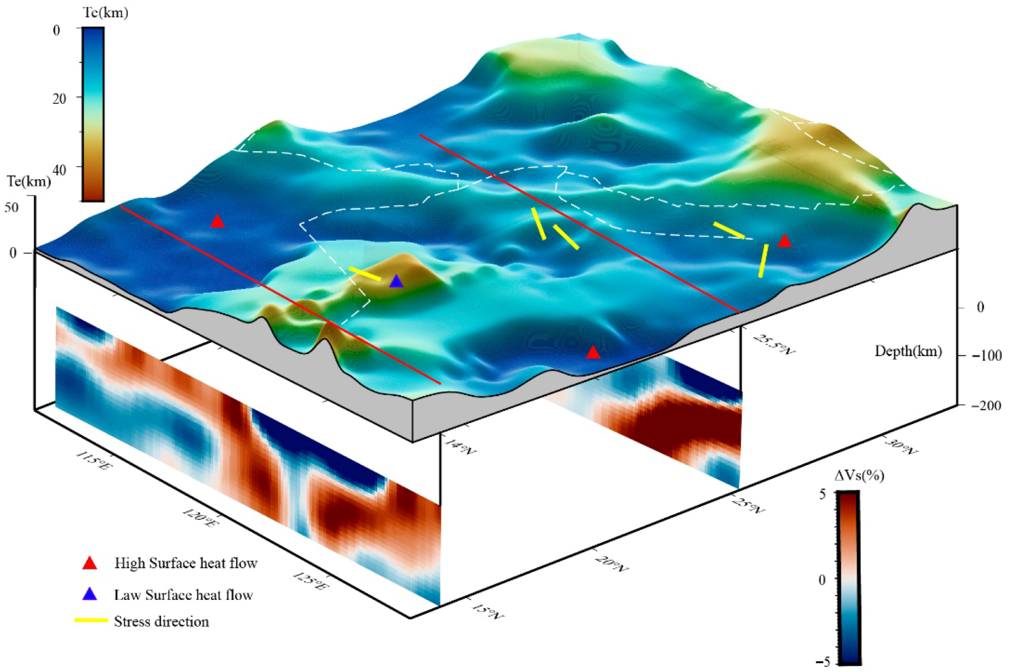
A coupling relationship exists between Te and the lithospheric thermal and deep velocity structures: regions of high Te correspond to elevated S-wave velocities and reduced heat flow at a depth of 100 km, indicative of robust lithospheric strength. Conversely, low Te aligns with diminished velocity anomalies and increased heat flow, suggesting lithospheric weakening. Statistical analysis reveals a moderate negative correlation between Te and heat flow (r = –0.44) and a weak positive correlation with the S-wave velocity anomaly at a depth of 100 km (r = 0.22). These results imply that the shallow thermal regime exerts a more significant influence on lithospheric strength in this region, whereas the impact of deep upper-mantle temperature on Te is comparatively limited (Figure 14). In oceanic crustal domains, Te is predominantly governed by thermal cooling processes. Both Te values and the overall age of the oceanic crust exhibit a systematic increase consistent with the classical crustal cooling and thickening model, primarily corresponding to the depth of the 200–400 °C isotherm. Local anomalies, such as those observed in the MTH region, display Te values exceeding those predicted by the cooling model, potentially reflecting the effects of underlying mantle thermal anomalies or convective dynamics.
Subduction systems play a critical role in modulating the spatial distribution of lithospheric strength. Dynamic topography-induced deflections can locally reduce Te by approximately 0–20 km. Our cross-sectional analyses demonstrate that spatial variations in Te correspond closely with subduction geometries (Figure 14). The spatial undulations of Te within the Taiwan and Philippine Sea blocks suggest that lithospheric mechanical structures have been shaped and inherited over geological timescales by factors such as subduction angle, slab bending, and tectonic thickening processes. The regional gradient of Te generally aligns with the orientation of the maximum principal compressive stress, with about 60% of data points exhibiting angular deviations less than 40°. This alignment indicates that large-scale spatial variations in lithospheric strength are broadly consistent with the prevailing tectonic stress field. Deviations from this trend may be attributed to perturbations induced by short-term tectonic events.

Author Contributions

Conceptualization, H.M. and G.Y.; methodology, H.M. and G.Y.; software, H.M.; validation, H.M., G.Y. and H.T.; formal analysis, H.M.; investigation, H.M., S.L. and Z.C.; resources, G.Y.; data curation, H.M. and T.Z.; writing—original draft preparation, H.M.; writing—review and editing, H.M., G.Y. and H.T.; visualization, H.M.; supervision, G.Y.; project administration, G.Y.; funding acquisition, G.Y. All authors have read and agreed to the published version of the manuscript.

Funding

This research was funded by the National Natural Science Foundation of China (NSFC) under grants (No. 42574074), Hubei Provincial Natural Science Foundation of China (2025AFB854), Scientific Research Fund from Institute of Seismology, China Earthquake Administration (IS202456377), and Research Grants from National Institute of Natural Hazards, Ministry of Emergency Management of China (202456377).

Data Availability Statement

The WGM2012 gravity model is available at https://bgi.obs-mip.fr/ (accessed on 15 October 2025). The 2025 GEBCO model is available at https://www.gebco.net/ (accessed on 13 October 2025). The CRUST1.0 model is available at https://igppweb.ucsd.edu/~gabi/crust1.html (accessed on 15 October 2025). The elastic thickness estimations were made using the open-source software product PlateFlex, available at https://github.com/paudetseis/PlateFlex (accessed on 10 May 2025). The World Stress Map is available at www.world-stress-map.org. Additional data are available from the corresponding author on request.

Acknowledgments

The authors express their sincere thanks to the journal editors and anonymous reviewers for their comments that improved the manuscript. The figures were prepared by using Generic Mapping Tools software 6.5.0.

Conflicts of Interest

The authors declare no conflicts of interest.

References

  1. Hsu, S.-K.; Wu, W.-N.; Lin, L.-K.; Wang, S.-Y.; Yeh, Y.-C.; Armada, L.T.; Dimalanta, C.B.; Chen, K.-T.; Tsai, Y.-J.; Tsai, C.-H. Segmentation of the Manila Subduction Zone and Slab Tearing beneath the Philippine Mobile Belt. J. Asian Earth Sci. 2025, 292, 106720. [Google Scholar] [CrossRef]
  2. Sibuet, J.-C.; Zhao, M.; Wu, J.; Lee, C.-S. Geodynamic and Plate Kinematic Context of South China Sea Subduction during Okinawa Trough Opening and Taiwan Orogeny. Tectonophysics 2021, 817, 229050. [Google Scholar] [CrossRef]
  3. Zhang, J.; Sun, Z.; Yang, H.; Zhang, F. A Model of Plate Bending at the Transition Zone From Subduction to Collision in Northernmost Manila Trench. Geophys. Res. Lett. 2022, 49, e2022GL100474. [Google Scholar] [CrossRef]
  4. Eakin, D.H.; McIntosh, K.D.; Van Avendonk, H.J.A.; Lavier, L.; Lester, R.; Liu, C.; Lee, C. Crustal-scale Seismic Profiles across the Manila Subduction Zone: The Transition from Intraoceanic Subduction to Incipient Collision. JGR Solid Earth 2014, 119, 1–17. [Google Scholar] [CrossRef]
  5. Wang, T.K.; Lin, S.-F.; Liu, C.-S.; Wang, C.-S. Crustal Structure of the Southernmost Ryukyu Subduction Zone: OBS, MCS and Gravity Modelling. Geophys. J. Int. 2004, 157, 147–163. [Google Scholar] [CrossRef]
  6. Ustaszewski, K.; Wu, Y.-M.; Suppe, J.; Huang, H.-H.; Chang, C.-H.; Carena, S. Crust–Mantle Boundaries in the Taiwan–Luzon Arc-Continent Collision System Determined from Local Earthquake Tomography and 1D Models: Implications for the Mode of Subduction Polarity Reversal. Tectonophysics 2012, 578, 31–49. [Google Scholar] [CrossRef]
  7. Gautier, S.; Tiberi, C.; Lopez, M.; Foix, O.; Lallemand, S.; Theunissen, T.; Hwang, C.; Chang, E. Detailed Lithospheric Structure of an Arc-Continent Collision beneath Taiwan Revealed by Joint Inversion of Seismological and Gravity Data. Geophys. J. Int. 2019, 218, 586–600. [Google Scholar] [CrossRef]
  8. Hutchings, S.J.; Mooney, W.D. Seismotectonics of the Philippine and Taiwan Subduction Systems and Implications for Seismic Hazards. Geochem. Geophys. Geosyst. 2024, 25, e2023GC010990. [Google Scholar] [CrossRef]
  9. Fan, J.; Zhao, D. P-wave Tomography and Azimuthal Anisotropy of the Manila-Taiwan-Southern Ryukyu Region. Tectonics 2021, 40, e2020TC006262. [Google Scholar] [CrossRef]
  10. Lu, Z.; Li, J.; Li, C.-F.; Du, X. Tectonic Controls on Effective Elastic Thickness of Lithospheres around the Southeast Asian Subduction Zones. Tectonophysics 2023, 863, 229994. [Google Scholar] [CrossRef]
  11. She, Y.; Zhao, Q.; Fu, G.; Meng, G.; Li, L.; Thant, M. Quantitative Estimation of the Effective Elastic Thickness around the Burma Plate and Correlation Analysis of Its Influencing Factors. Tectonophysics 2024, 886, 230434. [Google Scholar] [CrossRef]
  12. Billen, M.I. Modeling the Dynamics of Subducting Slabs. Annu. Rev. Earth Planet. Sci. 2008, 36, 325–356. [Google Scholar] [CrossRef]
  13. Karato, S. Mapping Water Content in the Upper Mantle. In Geophysical Monograph Series; Eiler, J., Ed.; American Geophysical Union: Washington, DC, USA, 2003; Volume 138, pp. 135–152. [Google Scholar]
  14. John Afelumo, A.; Li, C.-F.; Joshua Akinrinade, O.; Izuma Addey, C.; Antonio Capitanio, F. Spatial Variations in the Effective Elastic Thickness of the Indian Ocean Lithosphere. J. Asian Earth Sci. 2024, 276, 106315. [Google Scholar] [CrossRef]
  15. Li, Q.; Zhou, W.; Xu, B.; Chan, Y.; Tang, H.; Wu, Y. The Crust-Mantle Interaction of the Qiangtang Terrane: New Evidence from the Effective Elastic Thickness of the Lithosphere. Tectonophysics 2024, 890, 230510. [Google Scholar] [CrossRef]
  16. Chen, H.; Hsu, Y.; Ikuta, R.; Tung, H.; Tang, C.; Ku, C.; Su, H.; Jian, P.; Ando, M.; Tsujii, T. Strain Partitioning in the Southern Ryukyu Margin Revealed by Seafloor Geodetic and Seismological Observations. Geophys. Res. Lett. 2022, 49, e2022GL098218. [Google Scholar] [CrossRef]
  17. Lin, A.T.; Watts, A.B. Origin of the West Taiwan Basin by Orogenic Loading and Flexure of a Rifted Continental Margin. J. Geophys. Res. 2002, 107, ETG 2-1–ETG 2-19. [Google Scholar] [CrossRef]
  18. Mouthereau, F.; Petit, C. Rheology and Strength of the Eurasian Continental Lithosphere in the Foreland of the Taiwan Collision Belt: Constraints from Seismicity, Flexure, and Structural Styles. J. Geophys. Res. 2003, 108, 2002JB002098. [Google Scholar] [CrossRef]
  19. Chen, B.; Chen, C.; Kaban, M.K.; Du, J.; Liang, Q.; Thomas, M. Variations of the Effective Elastic Thickness over China and Surroundings and Their Relation to the Lithosphere Dynamics. Earth Planet. Sci. Lett. 2013, 363, 61–72. [Google Scholar] [CrossRef]
  20. Shi, X.; Kirby, J.; Yu, C.; Jiménez-Díaz, A.; Zhao, J. Spatial Variations in the Effective Elastic Thickness of the Lithosphere in Southeast Asia. Gondwana Res. 2017, 42, 49–62. [Google Scholar] [CrossRef]
  21. Yang, A.; Fu, Y. Estimates of Effective Elastic Thickness at Subduction Zones. J. Geodyn. 2018, 117, 75–87. [Google Scholar] [CrossRef]
  22. Lu, Z.; Audet, P.; Li, C.; Zhu, S.; Wu, Z. What Controls Effective Elastic Thickness of the Lithosphere in the Pacific Ocean? JGR Solid Earth 2021, 126, e2020JB021074. [Google Scholar] [CrossRef]
  23. Mao, X.; Wang, Q.; Liu, S.; Xu, M.; Wang, L. Effective Elastic Thickness and Mechanical Anisotropy of South China and Surrounding Regions. Tectonophysics 2012, 550–553, 47–56. [Google Scholar] [CrossRef]
  24. Font, Y.; Lallemand, S. Subducting Oceanic High Causes Compressional Faulting in Southernmost Ryukyu Forearc as Revealed by Hypocentral Determinations of Earthquakes and Reflection/Refraction Seismic Data. Tectonophysics 2009, 466, 255–267. [Google Scholar] [CrossRef]
  25. Kao, H.; Shen, S.J.; Ma, K. Transition from Oblique Subduction to Collision: Earthquakes in the Southernmost Ryukyu arc-Taiwan Region. J. Geophys. Res. 1998, 103, 7211–7229. [Google Scholar] [CrossRef]
  26. Malavieille, J.; Lallemand, S.E.; Dominguez, S.; Deschamps, A.; Lu, C.-Y.; Liu, C.-S.; Schnuerle, P.; Angelier, J.; Collot, J.Y.; Deffontaines, B.; et al. Arc-Continent Collision in Taiwan: New Marine Observations and Tectonic Evolution. In Geology and Geophysics of an Arc-Continent Collision, Taiwan; Geological Society of America: Boulder, CO, USA, 2002. [Google Scholar]
  27. Tan, E.; Lee, Y.-H.; Chang, J.-B.; Zheng, M.-J.; Shyu, C.J. Mountain Building Process of the Taiwan Orogeny. Sci. Adv. 2024, 10, eadp8056. [Google Scholar] [CrossRef]
  28. Tan, P.; Ding, W.; Li, J. Exhumation History of the Hengchun Ridge and Its Implications for Taiwan Orogenic Processes. Front. Earth Sci. 2022, 10, 941040. [Google Scholar] [CrossRef]
  29. Chiang, C.; Hsiung, K.; Yu, H. Two Types of Modern Sediment Dispersal Systems in the Western Taiwan Foreland Basin: Sediment Transfer from Basin to Basin. Depos. Rec. 2025, 11, 790–807. [Google Scholar] [CrossRef]
  30. Hsieh, A.I.; Vaucher, R.; MacEachern, J.A.; Zeeden, C.; Huang, C.; Lin, A.T.; Löwemark, L.; Dashtgard, S.E. Resolving Allogenic Forcings on Shallow-marine Sedimentary Archives of the Taiwan Western Foreland Basin. Sedimentology 2025, 72, 1755–1785. [Google Scholar] [CrossRef]
  31. Ling, Z.; Liu, H.; Zhao, L.; Zhang, T.; Li, C. The Effective Elastic Thickness of the Lithosphere Reveals Tectonic Process and Lithospheric Rheology of the Eurasian Basin. Terra Nova 2024, 37, 85–92. [Google Scholar] [CrossRef]
  32. Bonvalot, S.; Balmino, G.; Briais, A.; Kuhn, M.; Peyrefitte, A.; Vales, N.; Biancale, R.; Gabalda, G.; Reinquin, F. World Gravity Map: A Set of Global Complete Spherical Bouguer and Isostatic Anomaly Maps and Grids. Geophys. Res. Abstr. 2012, 14, 11091. [Google Scholar]
  33. Fullea, J.; Fernàndez, M.; Zeyen, H. FA2BOUG—A FORTRAN 90 Code to Compute Bouguer Gravity Anomalies from Gridded Free-Air Anomalies: Application to the Atlantic-Mediterranean Transition Zone. Comput. Geosci. 2008, 34, 1665–1681. [Google Scholar] [CrossRef]
  34. Stark, C.P.; Stewart, J.; Ebinger, C.J. Wavelet Transform Mapping of Effective Elastic Thickness and Plate Loading: Validation Using Synthetic Data and Application to the Study of Southern African Tectonics. J. Geophys. Res. 2003, 108, 2001JB000609. [Google Scholar] [CrossRef]
  35. Kirby, J.F.; Swain, C.J. An Accuracy Assessment of the Fan Wavelet Coherence Method for Elastic Thickness Estimation. Geochem. Geophys. Geosyst. 2008, 9, 2007GC001773. [Google Scholar] [CrossRef]
  36. Jiménez-Díaz, A.; Ruiz, J.; Pérez-Gussinyé, M.; Kirby, J.F.; Álvarez-Gómez, J.A.; Tejero, R.; Capote, R. Spatial Variations of Effective Elastic Thickness of the Lithosphere in Central America and Surrounding Regions. Earth Planet. Sci. Lett. 2014, 391, 55–66. [Google Scholar] [CrossRef]
  37. Ratheesh-Kumar, R.T.; Xiao, W. Effective Elastic Thickness along the Conjugate Passive Margins of India, Madagascar and Antarctica: A Re-Evaluation Using the Hermite Multitaper Bouguer Coherence Application. J. Asian Earth Sci. 2018, 157, 40–56. [Google Scholar] [CrossRef]
  38. Hrubcová, P.; Rastjoo, G.; Vavryčuk, V. Stress Variations in Southern Tonga Slab Derived From Deep-Focus Earthquakes. JGR Solid Earth 2024, 129, e2023JB028039. [Google Scholar] [CrossRef]
  39. Jiménez-Díaz, A.; Negredo, A.M.; Kirby, J.F.; Sánchez-Pastor, P.; Fullea, J.; Ruiz, J.; Pérez-Gussinyé, M.; Yu, C. The Mechanical Nature of the Lithosphere Beneath the Eastern Central Atlantic Hotspots. Geochem. Geophys. Geosyst. 2023, 24, e2022GC010608. [Google Scholar] [CrossRef]
  40. Straume, E.O.; Gaina, C.; Medvedev, S.; Hochmuth, K.; Gohl, K.; Whittaker, J.M.; Abdul Fattah, R.; Doornenbal, J.C.; Hopper, J.R. GlobSed: Updated Total Sediment Thickness in the World’s Oceans. Geochem. Geophys. Geosyst. 2019, 20, 1756–1772. [Google Scholar] [CrossRef]
  41. Uieda, L.; Barbosa, V.C.F.; Braitenberg, C. Tesseroids: Forward-Modeling Gravitational Fields in Spherical Coordinates. Geophysics 2016, 81, F41–F48. [Google Scholar] [CrossRef]
  42. Bai, Y.; Dong, D.; Kirby, J.F.; Williams, S.E.; Wang, Z. The Effect of Dynamic Topography and Gravity on Lithospheric Effective Elastic Thickness Estimation: A Case Study. Geophys. J. Int. 2018, 214, 623–634. [Google Scholar] [CrossRef]
  43. Husson, L. Dynamic Topography above Retreating Subduction Zones. Geology 2006, 34, 741. [Google Scholar] [CrossRef]
  44. Hayes, G.P.; Moore, G.L.; Portner, D.E.; Hearne, M.; Flamme, H.; Furtney, M.; Smoczyk, G.M. Slab2, a Comprehensive Subduction Zone Geometry Model. Science 2018, 362, 58–61. [Google Scholar] [CrossRef]
  45. Audet, P. PlateFlex: Software for Mapping the Elastic Thickness of the Lithosphere (Version v0. 1.0). Zenodo, 2019. Available online: https://zenodo.org/records/3576803 (accessed on 15 October 2025).
  46. Casallas, I.F.; Hu, J.-C. Effective Elastic Thickness in Northern South America. Appl. Sci. 2025, 15, 5163. [Google Scholar] [CrossRef]
  47. Zhao, F.; Zhan, C.; Pei, J.; Chen, Y.; Dai, M.; Hu, B.; Hou, L.; Ning, Z.; Xu, R. Spherical Gravity Inversion Reveals Crustal Structure and Microplate Tectonics in the Caribbean Sea. J. Mar. Sci. Eng. 2026, 14, 109. [Google Scholar] [CrossRef]
  48. Kirby, J.F.; Swain, C.J. Mapping the Mechanical Anisotropy of the Lithosphere Using a 2D Wavelet Coherence, and Its Application to Australia. Phys. Earth Planet. Inter. 2006, 158, 122–138. [Google Scholar] [CrossRef]
  49. Kirby, J.F. Estimation of the Effective Elastic Thickness of the Lithosphere Using Inverse Spectral Methods: The State of the Art. Tectonophysics 2014, 631, 87–116. [Google Scholar] [CrossRef]
  50. Forsyth, D.W. Subsurface Loading and Estimates of the Flexural Rigidity of Continental Lithosphere. J. Geophys. Res. 1985, 90, 12623–12632. [Google Scholar] [CrossRef]
  51. Laske, G.; Masters, G.; Ma, Z.; Pasyanos, M. Update on CRUST1.0—A 1-Degree Global Model of Earth’s Crust. In Proceedings of the EGU General Assembly 2013, Vienna, Austria, 7–12 April 2013. [Google Scholar]
  52. Audet, P. Toward Mapping the Effective Elastic Thickness of Planetary Lithospheres from a Spherical Wavelet Analysis of Gravity and Topography. Phys. Earth Planet. Inter. 2014, 226, 48–82. [Google Scholar] [CrossRef]
  53. Lu, Z.; Li, C.-F.; Zhu, S.; Audet, P. Effective Elastic Thickness over the Chinese Mainland and Surroundings Estimated from a Joint Inversion of Bouguer Admittance and Coherence. Phys. Earth Planet. Inter. 2020, 301, 106456. [Google Scholar] [CrossRef]
  54. Luo, F.; Yan, J.; Zhang, C.; Zhong, R.; Xie, X. The Effective Elastic Thickness of Lithosphere and Its Tectonic Implications in the South China Block. Acta Geosci. Sin. 2022, 43, 771–784. [Google Scholar] [CrossRef]
  55. Xu, G.; Chen, Z. Spatial Variations of Effective Elastic Thickness of the Lithosphere in the Okinawa Trough. J. Asian Earth Sci. 2021, 209, 104670. [Google Scholar] [CrossRef]
  56. Liu, W.; Li, C.; Zhu, S.; Lu, Z.; Wu, Z. Spatial Variations and Controlling Factors of the Effective Elastic Thickness of the Western Pacific Lithospheres. Chin. J. Geophys. 2021, 64, 1975–1986. [Google Scholar] [CrossRef]
  57. Guan, D.; Ke, X.; Wang, Y. Effective Elastic Thickness of the Lithosphere in the East and South China Seas and Adjacent Area Obtained Using the Convolution Method. J. Asian Earth Sci. 2019, 175, 247–255. [Google Scholar] [CrossRef]
  58. Zhu, W.; Liu, S.; Huang, S. Heat Flow in the Asian Continent and Surrounding Areas. Int. J. Terr. Heat Flow Appl. 2022, 5, 01–08. [Google Scholar] [CrossRef]
  59. Liu, C.; Banerjee, R.; Grand, S.P.; Sandvol, E.; Mitra, S.; Liang, X.; Wei, S. A High-Resolution Seismic Velocity Model for East Asia Using Full-Waveform Tomography: Constraints on India-Asia Collisional Tectonics. Earth Planet. Sci. Lett. 2024, 639, 118764. [Google Scholar] [CrossRef]
  60. Jiang, G.; Hu, S.; Shi, Y.; Zhang, C.; Wang, Z.; Hu, D. Terrestrial Heat Flow of Continental China: Updated Dataset and Tectonic Implications. Tectonophysics 2019, 753, 36–48. [Google Scholar] [CrossRef]
  61. Burov, E.B.; Diament, M. The Effective Elastic Thickness (Te) of Continental Lithosphere: What Does It Really Mean? J. Geophys. Res. 1995, 100, 3905–3927. [Google Scholar] [CrossRef]
  62. Watts, A.B.; Zhong, S.J.; Hunter, J. The Behavior of the Lithosphere on Seismic to Geologic Timescales. Annu. Rev. Earth Planet. Sci. 2013, 41, 443–468. [Google Scholar] [CrossRef]
  63. Su, J.; Zhu, W.; Li, G. Driven Magmatism and Crustal Thinning of Coastal Southern China in Response to Subduction. Solid Earth 2024, 15, 1133–1141. [Google Scholar] [CrossRef]
  64. Zhang, H.; Lü, Q.-T.; Wang, X.-L.; Han, S.; Liu, L.; Gao, L.; Wang, R.; Hou, Z.-Q. Seismically Imaged Lithospheric Delamination and Its Controls on the Mesozoic Magmatic Province in South China. Nat. Commun. 2023, 14, 2718. [Google Scholar] [CrossRef]
  65. Zhao, D.; Wang, J.; Huang, Z.; Liu, X. Seismic Structure and Subduction Dynamics of the Western Japan Arc. Tectonophysics 2021, 802, 228743. [Google Scholar] [CrossRef]
  66. Lo, C.-L.; Doo, W.-B.; Kuo-Chen, H.; Hsu, S.-K. Plate Coupling across the Northern Manila Subduction Zone Deduced from Mantle Lithosphere Buoyancy. Phys. Earth Planet. Inter. 2017, 273, 50–54. [Google Scholar] [CrossRef]
  67. Parsons, B.; Sclater, J.G. An Analysis of the Variation of Ocean Floor Bathymetry and Heat Flow with Age. J. Geophys. Res. 1977, 82, 803–827. [Google Scholar] [CrossRef]
  68. Watts, A.B.; Zhong, S. Observations of flexure and the Rheology of Oceanic Lithosphere. Geophys. J. Int. 2000, 142, 855–875. [Google Scholar] [CrossRef]
  69. Seton, M.; Müller, R.D.; Zahirovic, S.; Williams, S.; Wright, N.M.; Cannon, J.; Whittaker, J.M.; Matthews, K.J.; McGirr, R. A Global Data Set of Present-Day Oceanic Crustal Age and Seafloor Spreading Parameters. Geochem. Geophys. Geosyst. 2020, 21, e2020GC009214. [Google Scholar] [CrossRef]
  70. Ji, F.; Zhang, Q.; Zhou, X.; Bai, Y.; Li, Y. Effective Elastic Thickness of Zealandia and Its Implications for Lithospheric Deformation. Gondwana Res. 2020, 86, 46–59. [Google Scholar] [CrossRef]
  71. Chen, B.; Liu, J.; Chen, C.; Du, J.; Sun, Y. Elastic Thickness of the Himalayan–Tibetan Orogen Estimated from the Fan Wavelet Coherence Method, and Its Implications for Lithospheric Structure. Earth Planet. Sci. Lett. 2015, 409, 1–14. [Google Scholar] [CrossRef]
  72. Kalnins, L.M.; Watts, A.B. Spatial Variations in Effective Elastic Thickness in the Western Pacific Ocean and Their Implications for Mesozoic Volcanism. Earth Planet. Sci. Lett. 2009, 286, 89–100. [Google Scholar] [CrossRef]
  73. Wu, W.-N.; Lo, C.-L.; Lin, J.-Y. Spatial Variations of the Crustal Stress Field in the Philippine Region from Inversion of Earthquake Focal Mechanisms and Their Tectonic Implications. J. Asian Earth Sci. 2017, 142, 109–118. [Google Scholar] [CrossRef]
  74. Kuhasubpasin, B.; Moon, S.; Lithgow-Bertelloni, C. Unraveling the Connection between Subsurface Stress and Geomorphic Features. GSA Connect. 2024 2024, 56, 403730. [Google Scholar] [CrossRef]
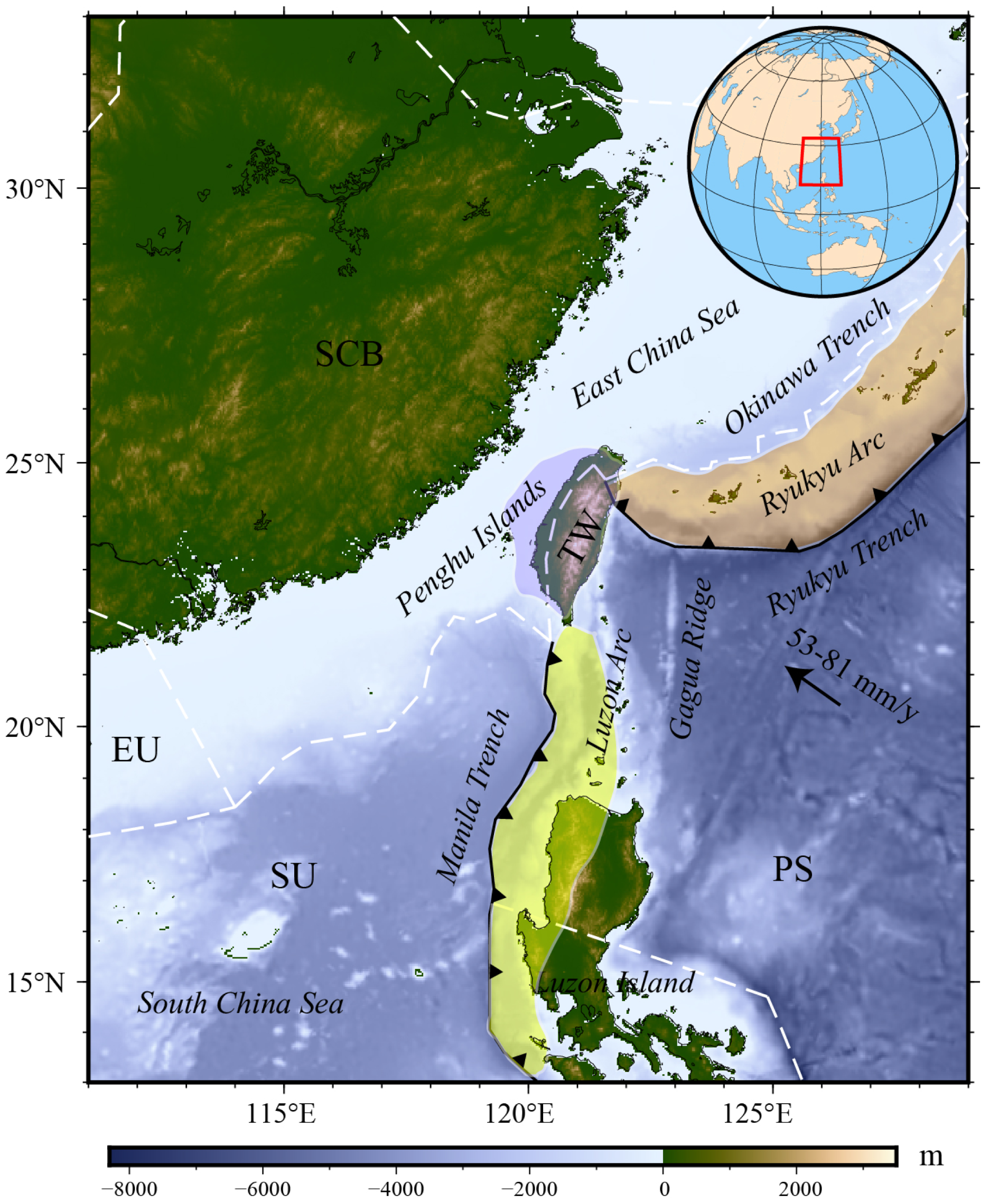
Figure 1. Tectonic environment of Taiwan. White dashed lines represent plate boundaries, black jagged lines represent trenches, and black arrows indicate the direction of plate movement. Bathymetric and topographic data are from are from 2025 GEBCO model (https://www.gebco.net/, accessed on 13 October 2025). TW: Taiwan; EU: Eurasian Plate; SU: Sunda Plate; PS: Philippine Sea Plate; SCB: South China Block. The yellow region represents the Manila subduction system, the orange region represents the Ryukyu subduction system, and the purple region represents the Taiwan orogen and foreland basin. The tectonic framework was adapted from [29]. The inset shows the overall location of the study area.
Jmse 14 00911 g001
Figure 2. Free-air gravity anomaly and Bouguer gravity anomaly data, with gravity anomaly data derived from the WGM2012 gravity model [32]. (a) Distribution of free-air gravity anomaly. (b) Distribution of Bouguer gravity anomaly.
Jmse 14 00911 g002
Figure 3. Sedimentary layer data from the GlobSed model [41]. (a) Sedimentary layer thickness. (b) Influence of sedimentary layer on Bouguer gravity.
Jmse 14 00911 g003
Figure 4. Corrected sedimentary correction results. (a) Corrected topographic distribution. (b) Corrected Bouguer gravity distribution.
Jmse 14 00911 g004
Figure 5. Effects of subduction blocks. (a) Dynamic topography caused by subduction blocks. (b) Bouguer gravity disturbance caused by subduction blocks.
Jmse 14 00911 g005
Figure 6. Elastic lithosphere thickness distribution. (a) Te distribution of uncorrected sedimentary layers. (b) Te error distribution of uncorrected sedimentary layers.
Jmse 14 00911 g006
Figure 7. Calculation results regarding corrected sedimentary layers. (a) Te distribution of corrected sedimentary layers. (b) Error distribution of Te in corrected sedimentary layers.
Jmse 14 00911 g007
Figure 8. Thermal structure data of the study area. (a) S-wave anomaly results at 100 km depth, corresponding to data from [59]. (b) Surface heat flow data, corresponding to data from the IHFC database (http://ihfc-iugg.org/, accessed on 12 December 2025) and [60]. MTH: Manila Trench Heat; RTH: Ryukyu Trench Heat; SCH: South China Block Heat; PSH: Philippine Sea Heat, TESH: Taiwan Eastern Sea Heat. These abbreviations correspond to representative heat-flow measurement points located in the South China Sea, Manila subduction zone, Ryukyu subduction zone, Philippine Sea region, and eastern offshore Taiwan, respectively. The black dashed circles represent regional data for selected typical marine heat flow points.
Jmse 14 00911 g008
Figure 9. Correlation coefficient results. (a) Correlation coefficient of Te with S-wave anomaly at a depth of 100 km, shown by blue dots. (b) Correlation coefficient of Te with surface heat flow, shown by red dots. In both panels, the black lines indicate the averaged values within each Te interval, and the green error bars represent the corresponding variability or uncertainty ranges.
Jmse 14 00911 g009
Figure 10. Elastic lithosphere thickness and oceanic crust age. The oceanic crust age data are from Seton et al. [69]. The mean Te values for sediment-corrected subduction regions within each 5 Ma oceanic age interval were statistically analyzed. The black solid line represents the mean value, and the shaded area indicates the range of values within one standard deviation of the statistical mean. The gray dashed lines represent the Te–age envelope curves for isotherms at 200, 400, 600, 800, and 1000 °C from the literature. SCH, MTH, PSH, TESH, and RTH correspond to heat flow measurement points in the South China Sea, Manila subduction zone, Philippine Sea subduction zone, southeastern waters of Taiwan, and Ryukyu subduction zone, respectively; the regions within a two-degree radius of each point were statistically analyzed.
Jmse 14 00911 g010
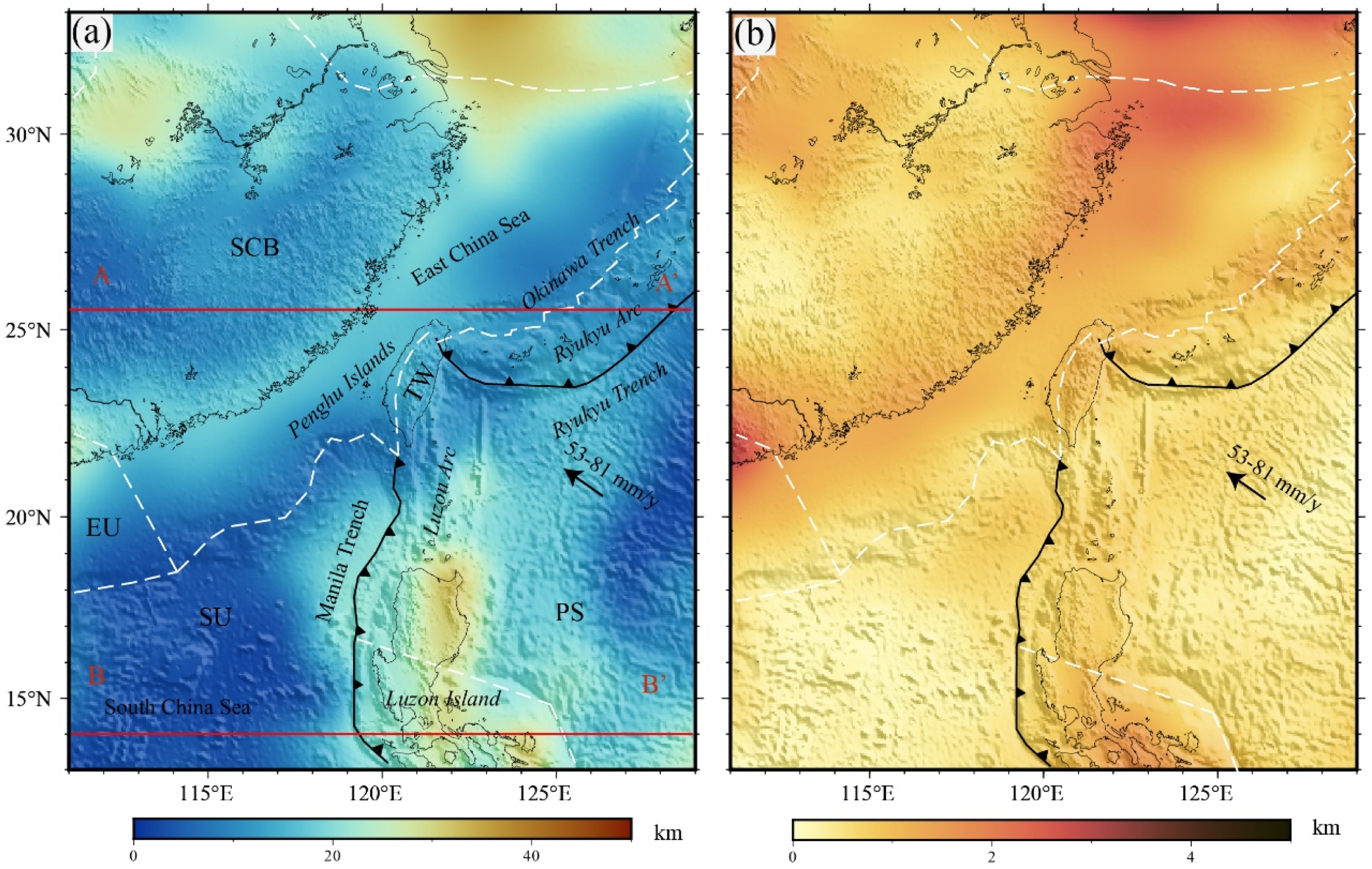
Figure 11. Profile A–A′ traverses northern Taiwan, whereas profile B–B′ crosses the Philippine Sea Plate. Results obtained after correction of the subduction block: (a) Corrected elastic lithosphere thickness distribution. (b) Corrected Te distribution error distribution.
Jmse 14 00911 g011
Figure 12. S-wave velocity anomaly profiles at depths of 0–200 km and Te (data from [59]): (a) BB’ profile results and (b) AA’ profile result.
Jmse 14 00911 g012
Figure 13. Comparison of principal stress direction and Te gradient direction. (a) Distribution of principal stress direction in WSM. (b) Error between Te gradient direction and principal stress direction. (c) Statistics regarding the deviation in stress direction angle.
Jmse 14 00911 g013
Figure 14. Schematic diagram of the impact of Te on Taiwan and neighboring areas. The red solid line represents the location of the extracted profile, which was taken from the subduction area in the figure. The profile represents the S-wave velocity anomaly at a depth of 0–200 km (based on data from [60]). The red triangles represent areas with relatively higher surface heat flow, the blue triangles represent areas with lower surface heat flow, and the yellow horizontal line represents the direction of stress.
Jmse 14 00911 g014
Table 1. Physical quantities and reference values.
Physical Quantity/UnitReference Value
Young’s modulus, E/(GPa)100
Gravitational constant, G/(m3/(kg·s2))6.67259 × 10−11
Poisson’s ratio, ν0.25
Gravitational acceleration, g/(m·s−2)9.8
Mantle density, ρm/(g·cm−3)3.27
Disclaimer/Publisher’s Note: The statements, opinions and data contained in all publications are solely those of the individual author(s) and contributor(s) and not of MDPI and/or the editor(s). MDPI and/or the editor(s) disclaim responsibility for any injury to people or property resulting from any ideas, methods, instructions or products referred to in the content.