A Hybrid LSTM-UDP Model for Real-Time Motion Prediction and Transmission of a 10,000-TEU Container Ship

Abstract

For various specialized maritime operations, predicting the future motion responses of structures is essential. For example, ship-borne helicopter landings require a predictable time frame of 6 to 8 s, while avoiding risks during ship navigation in waves calls for a 15-s prediction window. In this work, a real-time prediction method of future ship motions using the Long Short-Term Memory Neural Network (LSTM) is introduced. A direct multi-step output approach is used to continually update with the most recent data for prediction. This method can model the nonlinear time series of ship motions leveraging LSTM’s capabilities, and User Datagram Protocol (UDP) is used between devices to achieve low-latency data transfer. The performance of this framework is demonstrated and validated through multi-degree-of-freedom motion simulations of a 10,000-TEU container ship model in random waves. The results show that all the values of R² in the four cases are greater than 0.7, and the maximum and minimum values of R² correspond to predictable time scales of 6 s in Case I and 10 s in Case IV, respectively. This indicates that combining LSTM neural networks with the UDP protocol allows for accurate and efficient predictions and data transmission, and the calculating accuracy of the method decreases as the predictable time scale increases.

1. Introduction

The large amplitude motions of floating bodies in extreme sea conditions seriously affect the efficiency and safety of offshore operations, especially for special offshore operations [1,2]. To prevent and reduce accidents, the prediction of the motions of floating bodies for the next moment can provide a decision-making basis for people. Therefore, the real-time prediction of floating body motions has become a significant topic in the engineering field in recent years [3,4,5,6].

As is known, the real marine environment is characterized by random waves, and early prediction methods were mostly only applicable to time series models with strong linear and non-stationary features [7,8,9]. Nevertheless, the motions of floating bodies in extreme sea conditions are complex, and time series of motion usually have strong nonlinear and non-stationary characteristics. Therefore, the early numerical models were far from achieving the expected performance [10].

Over the past two decades, the emergence of deep learning models and artificial intelligence technology has transformed the marine engineering field, especially in predicting ship motions. It has been widely demonstrated that conventional deep learning models, such as support vector machines and random forests, are highly effective in processing extensive data and addressing complex nonlinear problems, leading to their widespread application in the prediction of floating structure motions. Panda et al. reviewed the applications of deep learning models in naval architecture and ocean engineering, showing that such models can significantly enhance performance and prediction efficiency in these fields [11]. However, these models require extensive data preprocessing and are limited in handling nonlinear and non-stationary problems.

Fortunately, related research has demonstrated that neural networks exhibit superior performance in nonlinear processing, achieving high predictive accuracy across various fields. Among different neural network types, the predictive strength of LSTM stems from its ability to learn long-term dependencies in complex, non-stationary time series. This capability is crucial for predicting tasks where future states are determined by past events, a challenge that traditional RNNs often fail to address.

Furthermore, both Gated Recurrent Unit (GRU) and LSTM are capable of capturing long-term dependencies, rendering them well-suited for time-series problems. Notwithstanding this, the increased complexity of the LSTM architecture directly translates to its enhanced efficacy in modeling such temporal dependencies. Mateus et al. reported that though GRU slightly surpassed its LSTM counterpart in select scenarios, LSTM has more competitiveness [12]. Buestán-Andrade et al. demonstrated that the LSTM model exhibited consistent superiority over the GRU, with a lower RMSE (347.9 kWh vs. 394.8 kWh). Additionally, in their study, LSTM’s training time was 10 s shorter, further suggesting higher efficiency when prediction accuracy is prioritized [13]. Moreover, according to Gers et al., the forget gate in the LSTM architecture addresses the issue of gradient vanishing, which arises from the chain rule of calculus during backpropagation through time [14]. Thus, given the strong memory effect and the consequential influence of past waves in marine structure motion, accurately modeling its nonlinear, long-term dependencies is crucial. For this purpose, the LSTM model is selected for its proven capability in handling such complex temporal dynamics.

The real-time motion prediction of floating structures in realistic sea conditions presents multiple obstacles: a scarcity of real ship data, the impracticality of pre-training, lengthy computation times, and significant data latency, all of which hinder effective application. Whereas the authors’ previous work predicted the future motion responses of a warship using calculated data [3], the present study leverages real-world motion records of a 10,000-TEU container ship. The main novelty of this work is the assessment of the model’s generalization capability with this real dataset, thereby advancing the prior theoretical findings toward practical engineering applications. The implementation of a User Datagram Protocol facilitates real-time data transmission across devices. The model can accurately predict the ship’s roll, pitch, and heave responses for the next 6–10 s, providing synchronous results. The key achievements of this work and suggestions for future research are summarized in the conclusion section.

2. Theoretical Background

2.1. Hydrodynamic Methods in the Framework of Potential Flow Theory

During the navigation of the vessel, due to the wave excitation, the ship will experience 6 degrees of freedom (DOF) motion. The focus of this work is on real-time prediction and transmission of the heave, roll, and pitch responses of ships for the next 6–10 s. According to Newton’s laws, under the wave excitation, the motions of a ship in waves can be viewed as a forced vibration.

$$\left[a\right]\left\{{\ddot{\eta }}_r(t)\right\}=\left\{F(t)\right\}$$

(1)

where [a] denotes the generalized structural mass matrix. $\left\{{\eta }_r(t)\right\}$ denotes the rigid ship motions in waves. $r=1,2\cdots 6$ denotes the 6-DOF rigid motions. $\left\{F(t)\right\}$ denotes the fluid forces, including the incident wave force, radiation force, diffraction wave force, hydrostatic restoring force, and slamming force. Having obtained the fluid forces acting on the hull, the instantaneous ship motion equation in waves can be formulated as follows [15,16]:

$$(\left[a\right]+\left[\mu \left(\infty \right)\right])\left\{{\ddot{\eta }}_r(t)\right\}+{\displaystyle {\int }_0^t[K(\tau )]\left\{{\dot{\eta }}_r(t-\tau )\right\}d}\tau +\left[C\right]\left\{{\eta }_r(t)\right\}=\left\{F_I(t)\right\}+\left\{F_D(t)\right\}+\left\{F_f(t)\right\}$$

(2)

where $\left[\mu \left(\infty \right)\right]$ denotes the added mass as $\omega \to \infty$. $[K(\tau )]$ denotes the memory function. $\left[C\right]$ denotes the hydrostatic coefficient. $F_I(t)$ denotes the incident wave force. $F_D(t)$ denotes the diffraction wave force. $F_f(t)$ denotes the slamming force.

Finally, the fourth-order Runge–Kutta method is employed to obtain the 6-DOF motions of ships.

2.2. Basic Concepts of the LSTM Model

The LSTM model distinguishes itself from traditional RNNs through its gated architecture, which is composed of input, forget, and output gates (denoted as i_t, f_t, and o_t, respectively). This structure collectively regulates the internal state of each neuron across time steps. The operation mechanism of the LSTM neurons is illustrated in Figure 1. Via the cell state, the neurons retain input data from previous time steps. Through this gating mechanism, the temporal dependency between successive outputs is effectively reduced to a linear superposition of multiple independent functions, rather than being represented by a composite function. As a result, long-time series data can be effectively stored, and the likelihood of gradient explosion or vanishing is significantly reduced during gradient computation.

As illustrated in Figure 1, based on the input sequence x = (x₁, x₂, …, x_t), the time series of hidden state h = (h₁, h₂, …, h_t) and output y = (y₁, y₂, …, y_t) can be obtained, respectively. In this work, the past motion data x = (x₁, x₂, …, x_t) is used as input data, and the predicted future ship motion y = (y₁, y₂, …, y_t) is used as output data. $c_t$ denotes the unit state at the t-th moment. ${\tilde{c}}_t$ indicates the temporary status.

The forget gate (f_t), is responsible for the selective removal of information from the previous cell state.

f_t = σ (W_f · [h_t−1, x_t] + b_f)

(3)

where W_f, h_t−1, x_t, and b_f represent the weight matrix of the forget gate, the previous hidden state, the present input, and the offset vector of the forget gate, respectively.

The input gate i_t is responsible for the information added to the current cell:

i_t = σ (W_i · [h_t−1, x_t] + b_i)

(4)

$${\tilde{c}}_t=\tanh (W_c·[h_{t-1},x_t]+b_c)$$

(5)

where W_i and b_i are the weight matrix and offset vector of the input gate. W_c and b_c are the weight matrix and offset vector of the current cell state. ${\tilde{c}}_t$ is the temporary state. and σ and tanh denote the activation functions:

σ(x) = 1/(1 + e^−x)

(6)

tanh(x) = (e^x − e^−x)/(e^x + e^−x)

(7)

The output gate o_t is responsible for the information exported from the current cell:

o_t = σ (W_o · [h_t−1, x_t] + b_o)

(8)

where W_o and b_o denote the weight matrix and offset vector of the output gate.

The updated cell state at the current time step enables the network to retain information from previous moments. This state, denoted as c_t, is computed from the previous cell state c_t−1 and a temporary candidate state ${\tilde{c}}_t$ during the network’s operation.

$$c_t=f_t\cdot c_{t-1}+i_t\cdot {\tilde{c}}_t$$

(9)

The current cell state c_t does not simply replicate the previous state c_t−1. Instead, the cell state c_t represents the current memory of the cell, inherited from the previous state c_t−1. As illustrated in the LSTM unit (as shown in Figure 2), the update of c_t combines a filtered version of the old memory with the processed new input. Specifically, the forget gate determines what portion of c_t−1 to retain by assigning corresponding weights, while the input gate regulates the incorporation of new information. The updated cell state is then selectively output via the output gate. Crucially, this design mitigates the vanishing and exploding gradient problems because the cell state update employs an additive structure, as opposed to the recurrent multiplicative structure of standard RNNs. This additive property prevents the exponential decay or growth of gradient magnitudes during backpropagation through time.

The output of the current cell state c_t is used to export the final learning results. h_t denotes the current hidden state, which can be expressed as:

h_t = o_t ⊙ tanh(c_t)

(10)

After the LSTM completes the sequence feature extraction, the resulting encoded representations are passed to a fully connected layer to compute the network’s final output, which can be presented as follows:

$$y_t=\varphi \left(W_{y}h+b_y\right)$$

(11)

In an LSTM model applied to ship motion prediction, the output y_t denotes the predicted future motions, serving as the target variable. Wy and by represent the weight matrix and offset vector of predicted future motions.

The design of the prediction model’s central component is directly derived from the aforementioned LSTM principles. To determine the hyperparameters of LSTM, a series of single-variable tests were conducted. In this study, the LSTM architecture consisted of an input layer (input_size = 1), two hidden layers with 20 neurons respectively (hidden_size = 20), and a fully connected output layer (output_size = 1). To mitigate overfitting, a dropout rate of 0.2 is utilized. The model is optimized employing the Adam algorithm with a learning rate of 0.006, using mean squared error as the loss function. The dataset is divided into training and testing sets, with 80% of the samples allocated to training and the remaining 20% to testing. In this study, a time step of 0.1 s is adopted, with the data volume ratio between input and output maintained at 10:1. For instance, using 100 input data points to predict 10 target values corresponds to leveraging 10 s of historical data to predict 1 s of future motion. To meet the practical requirement of predicting 10 s from 100 s of prior data, the model is configured with a fixed window length of 1000 points, corresponding to a 10:1 data ratio. In the absence of a universal standard for the input-output window ratio—a choice supported as experience-driven by prior work [3,17,18,19]—our decision is guided by two key factors: the high sampling rate of the ship motion data and the LSTM’s inherent need for extended context to establish long-term dependencies. An inadequate window length would diminish predictive performance. Thus, a 10:1 ratio is implemented to satisfy these requirements. The model parameters are subsequently optimized by evaluating prediction outcomes against performance indicators, resulting in a robust parameter set that achieves the targeted engineering accuracy.

In addition, to mitigate the influence of varying data scales, a normalization approach is applied to the training data. To accurately assess model performance on the original data distribution, the predictions generated on the test set are reverted via inverse normalization. All evaluation metrics are subsequently computed using the denormalized values.

2.3. Principle of Prediction of Ship Motion Using the LSTM Model

The LSTM model can be viewed as a complex, unknown function. Historical ship motion data, which serves as the independent variable, is fed into this function to train the LSTM model and iteratively adjust its parameters. Therefore, establishing the LSTM model forms the basis for predicting future ship motions. The process involves three main steps: first, known ship motion data is input to train the model; next, the model parameters are updated in each iteration, allowing it to learn and capture patterns in the data; ultimately, the trained model is deployed to generate multi-second predictions of the ship’s motion data.

To illustrate the underlying principle of future data prediction, consider the simple linear regression model as an example. In such cases, Equation (12) is typically employed to fit a series of observed data points, thereby generating predicted future values.

$$f_{w,b}\left(x\right)=wx+b$$

(12)

where $f_{w,b}\left(x\right)$ is the predicting function. x is the input variable. Both x and f(x) are known values, which are the undetermined parameters. Initially, the weight w and bias b parameters of function f(x) are randomly initialized to form the preliminary prediction model, which is applied to the training data for fitting. The quality of the fit under the current parameters is quantified using the loss function (Loss) and the goodness of fit (R²). Following each training iteration, error feedback derived from these metrics on the validation set is propagated backwards through the model. Based on this feedback, gradients are computed via the backpropagation algorithm, and an optimizer iteratively adjusts w and b. This cycle continues until all evaluation metrics stabilize and the error is minimized, at which point the optimal parameters are obtained, constituting a prediction function that achieves optimal data fitting. Then the future ship motions can be predicted by f(x).

The calculation effect is reflected by the goodness of fit (R²) and loss function (Loss). The goodness of fit can be written as:

$$R^2=1-{\displaystyle \frac{{\displaystyle \sum _{i=1}^n{\left({\widehat{y}}_i-y_i\right)}^2}}{{\displaystyle \sum _{i=1}^n{\left(y_i-\overline{Y}\right)}^2}}}$$

(13)

As shown in Equation (13), the goodness-of-fit improves as the R² value approaches 1, with values closer to 1 indicating a superior fit of the model to the data. y_i is the actual values. ${\widehat{y}}_i$ is the prediction values. $\overline{Y}$ is the mean values.

In a comprehensive investigation of loss functions for time-series regression, Abbasimehr and Paki highlighted key considerations for modeling ship motion responses. They demonstrated that the Mean Absolute Error (MAE) produces disproportionately large gradients for the small values typical of ship motions, which can adversely affect the learning process. Furthermore, they noted that Huber loss, while robust, is less sensitive to outliers compared to Mean Squared Error (MSE). This reduced sensitivity may, in certain cases, hinder the model from achieving the high level of training accuracy required for precise motion prediction [20]. Thus, compared with the MAE and Huber loss, the MSE is a more suitable loss function in deep learning [21].

$$LOSS={\displaystyle \frac{1}{n}}{\displaystyle \sum _{i=1}^n{({\widehat{y}}_i-y_i)}^2}$$

(14)

where ŷ_i is the output variable, that is, the predicted values. y is the actual value. n is the total number of training samples.

To train the LSTM model, the known input data and corresponding expected output data are fed into the network. It should be noted that in each iteration, the parameters (e.g., weights w and biases b) need to be updated simultaneously to refine the model. After sufficient training, optimal parameters w and b are obtained by minimizing the loss function, enabling the model to fit the training data well. Subsequently, the trained model can be used with new, unseen input data x to predict the corresponding output y.

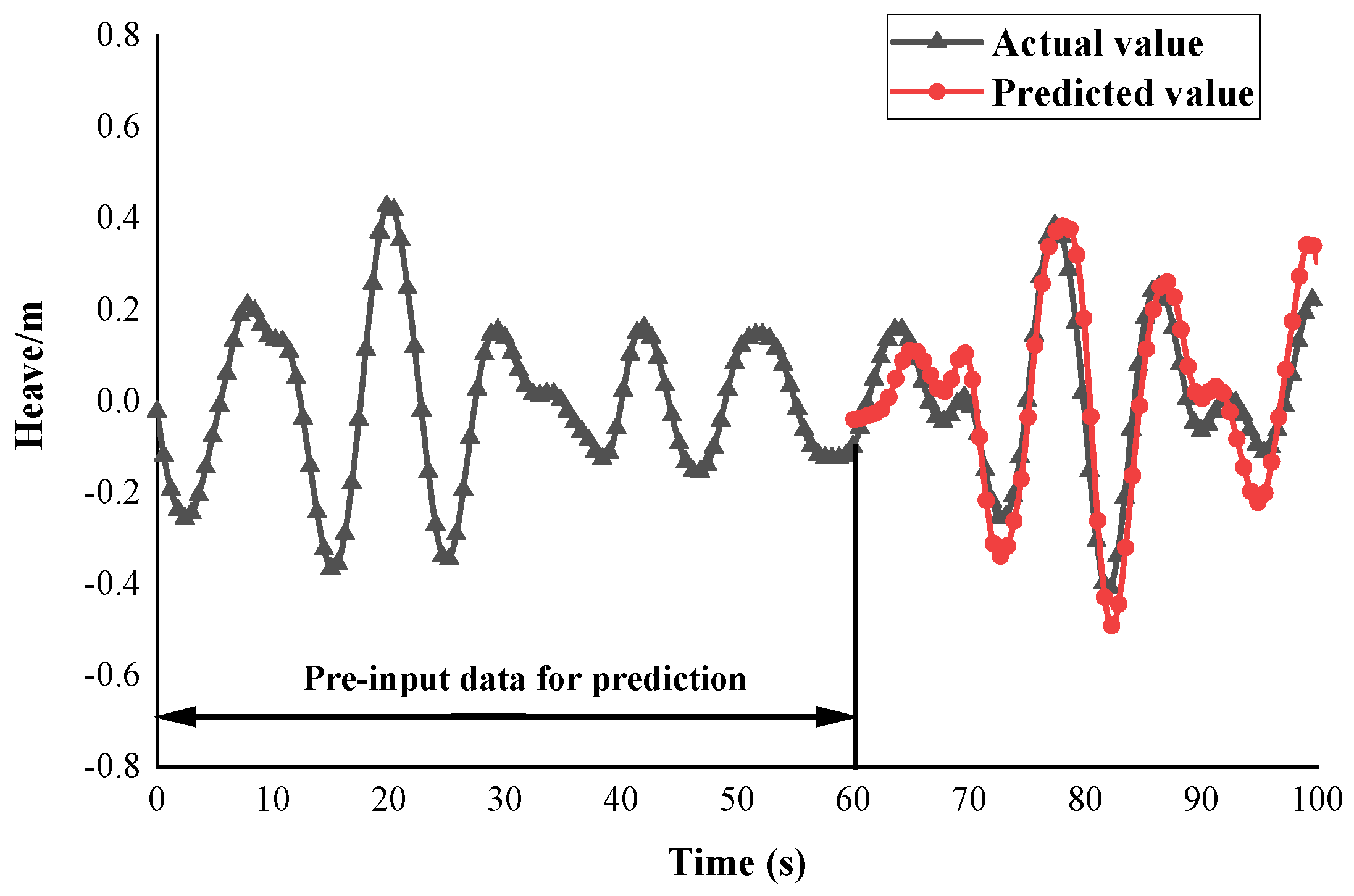
In addition, a direct multi-step-ahead prediction strategy is adopted in this study, as shown in Figure 2. It can be seen that the input sequence X = {x₁, x₂, …, x_M−1, x_M} represents the known data, while the output sequence Y = {y₁, y₂, …, y_N−1, y_N} corresponds to the predicted values. This method leverages the latest available data for each prediction step, and crucially, each predicted value is independent of previous predictions in the sequence. This method effectively addresses the challenge of prediction errors compounding over time, thereby enhancing long-term reliability [22].

2.4. Set-Up and Training of Prediction Model

The development and testing are carried out on a Lenovo Savior Y7000P-15 laptop, utilizing Python 3.8.2 and PyCharm Community Edition 2020.1.2. The system is equipped with an Intel Core i7-13700HX processor, 16 GB of RAM, 1 TB of storage, and an NVIDIA GeForce RTX 4060 GPU (8 GB VRAM). The model requires only that the PyTorch and CUDA versions are compatible, with no other specific dependencies. The specific libraries used are listed in

Table 1. Libraries used in this work.

Library ID	The Name of the Library
1	File and Path Operations Libraries import os import shutil
2	Data Serialization and Network Communication Libraries import struct import socket
3	Iterator Utilities Library from itertools import chain
4	PyTorch Deep Learning Libraries import torch.nn.init as init import torch import torch.nn as nn import torch.nn.functional from torch.utils.data import DataLoader
5	Numerical Computing and Data Manipulation Libraries import numpy as np import pandas as pd
6	Random Number and Excel I/O Libraries import random import openpyxl

. With the LSTM architecture established, the overall ship motion prediction model can be subsequently assembled.

2.4.1. Dataset Description and Preprocessing

The study is based on a full-scale ship motion dataset, collected using an integrated high-precision navigation and motion sensor system. The system, consistent with industry standards, combines an Inertial Measurement Unit (IMU) with a GNSS receiver. The data was recorded at a fixed sampling frequency of 20 Hz over a total duration of 2000 s, resulting in 40,000 consecutive samples for each DOF motion.

Prior to model training, the raw signals undergo a standardized preprocessing pipeline to ensure data quality and relevance. The raw time-series for each DOF, stored as a one-dimensional array, first undergo the essential preprocessing: a low-pass Butterworth filter (cut-off: 2 Hz) is applied to isolate wave-frequency motions, followed by the removal of statistical outliers (beyond ±4 standard deviations from a moving median) via linear interpolation. To prepare the data for the neural network, a normalization step is performed. Contrary to common zero-mean scaling, the min–max method is specifically employed to scale all values to the range [0, 1] according to Equation (15), using the minimum and maximum values from the training set:

x′ = (x − min_i)/(max_i − min_i)

(15)

The minimum and maximum values of each DOF motion in the training set are retained for subsequent application.

With normalization completed, the data is segregated into an 80-20 split for training and testing purposes. The final preprocessing step involves converting both sets into the LSTM-compatible format and, simultaneously, transforming the raw sequential data into input-output pairs for supervised learning. The input-output pairs, which define the mapping from current to target sequences, are defined by the systematic application of a fixed-length sliding window across the time series. During this process, each window position yields an input sequence x (a slice of the data) and a corresponding output sequence y. The overall data structure is thereby transformed from a list of values into a tensor for model consumption.

2.4.2. Model Development and Optimization

The overall LSTM architecture is constructed by programming and invoking dedicated LSTM modules. Hyperparameters of the model are determined based on preliminary single-variable experimentation. With both cell and hidden states commencing from a zero initial condition, the model is trained on the prepared data. The optimization process, governed by the loss function in Equation (14), is carried out via the Adam optimizer to perform gradient descent. Finally, the model is applied to the test set to generate predictions and compute the corresponding error.

2.4.3. Model Deployment Preparation

With training completed, the parameters are saved to a checkpoint file. This file is then loaded to initialize the model for making predictions on new data. The predictions on the training set, together with the actual values, are stored in a dedicated array for comparative analysis. This process completed the training for one DOF. The same procedure is then repeated sequentially to train models for each subsequent DOF.

3. Data Transmission Using the UDP Protocol

This study employed a virtual simulation platform developed in MATLAB R2024b/Simulink to emulate the prediction and transmission of ship motion data during actual carrier-based aircraft landing operations, as illustrated in Figure 3. It continuously receives the latest motion data, generates predictions immediately, and transmits the results without delay. To facilitate this data transmission, UDP is employed as the communication protocol between devices.

The prediction module is designed to train and predict only one DOF at a time. The prediction algorithm employs a dual-loop architecture: an outer loop that iterates over the temporal sequence, and an inner loop that cycles through DOF at every time step. Within the inner loop, predictions for all DOF are generated based on the current input data. The outer loop continuously acquires new real-time data and advances the prediction to the next time step. This structure has no predefined stopping condition, enabling the system to run indefinitely. The detailed steps of the prediction process are as follows.

3.1. UDP Communication Initialization

First, the motion prediction and transmission systems are configured with a dedicated UDP data pipeline to enable real-time data exchange. The advantage of UDP lies in its low latency, which stems from its connectionless design and lack of retransmission mechanisms. For the UDP, data is packaged and transmitted directly, minimizing protocol overhead and making it particularly suitable for real-time applications. UDP offers more predictable and controllable delays under stable network conditions. This makes it well-suited for the real-time “data collection→model prediction→result transmission” pipeline in ship motion prediction. Although data transmission inherently involves some delay—early experiments indicated a latency of approximately 3 s—subsequent network and equipment upgrades significantly reduced this delay to a nearly negligible level, and the overall impact of latency was minimal.

A continuous data flow is established where the transmission system pushes the latest motion vector to the prediction system’s socket every 0.05 s. The prediction system, in turn, ingests this data at half the frequency (0.1-s intervals), thereby processing alternate packets to create a sufficient time buffer for completing its prediction and communication cycles.

3.2. Data Update and Accumulation

The system is designed to predict ship motion for a horizon of 6 to 10 s. Given the 10:1 input-to-output ratio, predicting 10 s of output requires 100 s of input data. Therefore, A real-time data pipeline is established from the transmission system to the prediction system. Initially, when the total data history is less than 100 s, a dual-path routing mechanism is activated, directing each new data entry to be stored in both the prediction set and the growing received dataset. Once the total data history exceeds 100 s, the prediction set retains only the most recent 100 s of data, while the received dataset continues to grow by incorporating all incoming data, thereby providing a complete record of all data received.

3.3. Normalization of Prediction Set Data

The data loader is invoked to retrieve the minimum and maximum values of the current DOF motion from the training set, which are recorded during the training phase, enabling normalization of the prediction set data.

To facilitate real-time online prediction and transmission, the prediction set is normalized using the min–max values derived from the training set, ensuring that all motion data remains on a consistent scale during prediction. Directly applying the minimum and maximum values derived from the test set at each prediction step constitutes a form of data leakage. This practice can contaminate the prediction process by introducing significant distributional bias [23]. Therefore, applying a unified standard for data processing throughout the prediction process is essential. In this work, the approach of adopting the training set’s min–max values as the consistent normalization benchmark is implemented, as illustrated in Figure 4.

3.4. Model Prediction and Data Processing Workflow

Prior to prediction, the cell state and hidden state must be initialized as zero vectors. The trained model parameters are loaded from saved files, and the model is reconstructed and updated to create the predictive model for each DOF. Prediction is then performed on the normalized data. Since the resulting predictions also lie within the [0, 1] range, inverse normalization (denormalization) is applied to convert them back into actual physical values.

Following the completion of motion forecasts for all degrees of freedom, the ship’s roll, pitch, and heave for the 6–10 s horizon are obtained. These values, together with their corresponding timestamps, are assembled into a structured five-column matrix (Time, Heave, Pitch, Roll). The most recent entry (final row) of this matrix is then appended to both the prediction results repository and the transmission dataset for downstream tasks.

3.5. Real-Time Data Transmission and Archiving

A real-time data link is established, leveraging the UDP protocol to connect the motion prediction system with the downstream result visualization and comparison system. The latter real-time displays all data involved in each prediction cycle, synchronizing with the motion data transmission system. The display system ingests data from the prediction system and executes a real-time comparative analysis, generating a dynamic overlay of the latest forecasts against their corresponding measured values for immediate visualization.

After the above steps are completed, one full prediction cycle concludes. The entire process of data prediction and transmission is designed to finish within 0.1 s. This allows the motion prediction system to receive a new batch of data after 0.1 s and initiate a subsequent prediction cycle, thereby sustaining a continuous, rolling prediction process. Additionally, the system periodically archives the complete set of received data and the transmitted prediction results into two distinct sheets within an Excel file.

4. Result Presentation and Discussion

A 10,000-TEU container ship is chosen as the research object. Length overall is 316 m. Breadth is 40.9 m. Depth is 30.9 m. Draft is 13.4 m. Displacement is 100,721.2 tons. The representative calculated work conditions are shown in

Table 2. Calculated work conditions.

Case ID	Forward Speed U (knot)	Significant Wave Height H1/3 (m)	Spectral Peak Period TZ (s)	Heading Angle β (°)
Case-I	10	6	9.5	0
Case-II	10	10	11	45
Case-III	14	6	9.5	0
Case-IV	14	10	11	45

.

4.1. Comparison Between the Proposed Model and Other Models

Predicting ship motion in real sea conditions involves several challenges, including limited availability of real ship data, inability to conduct pre-training, considerable time consumption, and significant latency in the prediction outputs. Therefore, to evaluate the performance in predicting motion data for the next 6 s, this section conducts a comparative analysis between the present model and two other neural network models—GRU and Radial Basis Function (RBF). By comprehensively considering both prediction accuracy and computational speed, we aim to identify the most effective approach for ship motion prediction in complex and random real-sea conditions. The hyperparameter settings of the three neural network models are provided in

Table 3. Hyperparameter settings of three models.

Model	Number of Neurons	Hidden Layer	Activation Function	Learning Rate	Iterations
LSTM	20	2	Tanh(x)	0.006	150
RBF	20	2	Radial basis function	0.006	150
GRU	20	2	Tanh(x)	0.006	150

. The activation functions for the hidden layer nodes are selected as the optimal choice for each model based on experimental results, while all other parameters are kept consistent across the models.

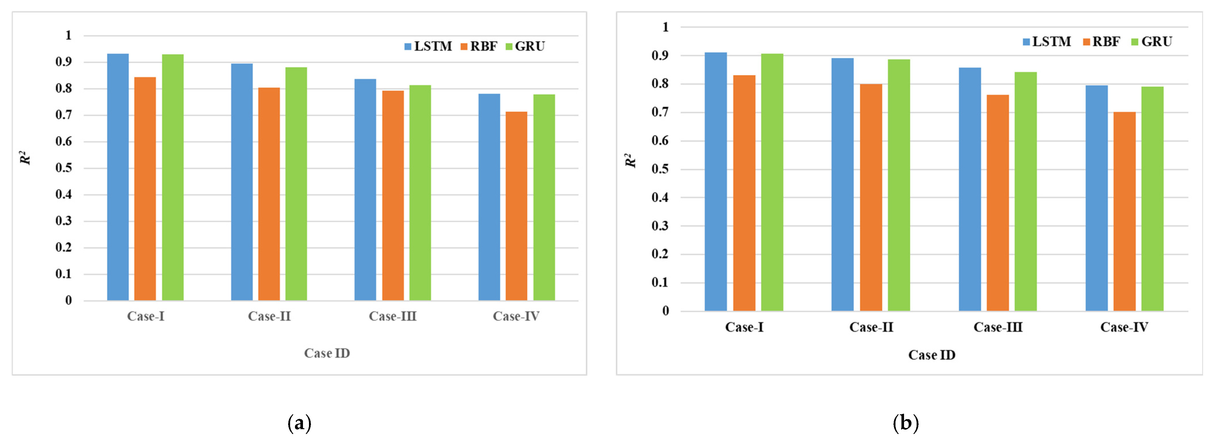
The comparative results of heave and pitch motions in Figure 5 reveal a clear performance hierarchy (LSTM > GRU > RBF) in predicting ship motions in the four cases. The supremacy of the LSTM model stems from its triple-gate mechanism (input, forget, output), which provides strong adaptability and precise control over long-range dependencies in time-series data. The GRU model, with a simplified two-gate structure and the absence of a dedicated forget gate, along with the RBF network—a type of fully connected network not specialized for sequential data—are less suited for such tasks, resulting in their relatively lower predictive performance.

Next, the computational efficiency of the three models is compared. The results across the four cases exhibited broadly consistent trends, and for clarity, only Case-I is presented as a representative case, as summarized in

Table 4. Comparison of computational efficiency of three models in Case-I.

Model	Data Volume (Training/Prediction)	Time Consumption of Training	Time Consumption of Prediction (s)
LSTM	32,000/8000	1 h 45 min	0.08
RBF	32,000/8000	1 h 39 min	0.07
GRU	32,000/8000	1 h 47 min	0.09

. It should be noted that computational efficiency is closely tied to the computing environment, and the results reported here are obtained under the specific setup used in this study. The prediction set comprised 8000 data points sampled at intervals of 0.05 s. As shown in Table 4, the training and prediction times required by the three models are generally comparable, with the time for a single prediction round not exceeding 0.1 s. Among the models, RBF demonstrated the highest computational efficiency. Although RBF marginally outperformed LSTM in this regard, the difference is slight, underscoring LSTM’s continued competitiveness in computational performance. This finding aligns closely with the conclusion drawn by Buestán-Andrade et al. [13].

4.2. Comparison Among Multi-Time Scale-Predicted Results

In this work, the past motion records are taken as input data, and the target motions in the future are taken as output data. A time difference can be observed between the past motions and target motions, and the time difference is the predictable time scale that can be determined through the model. In this section, the predictable time scale is taken as 6 s and 10 s.

The time scale required for various specialized maritime operations depends on the specific nature of these operations. For example, a carrier-based helicopter landing requires a predictable time scale of 6–8 s, while risk mitigation for ships navigating in waves requires a time scale of 15 s. Therefore, predictable time scales of 6 s and 10 s are selected for real-time prediction of ship motion at multiple time scales. To ensure high accuracy under random wave conditions, the duration of pre-input data is set to 60 s and 100 s, corresponding to the predictable time scales of 6 s and 10 s, respectively.

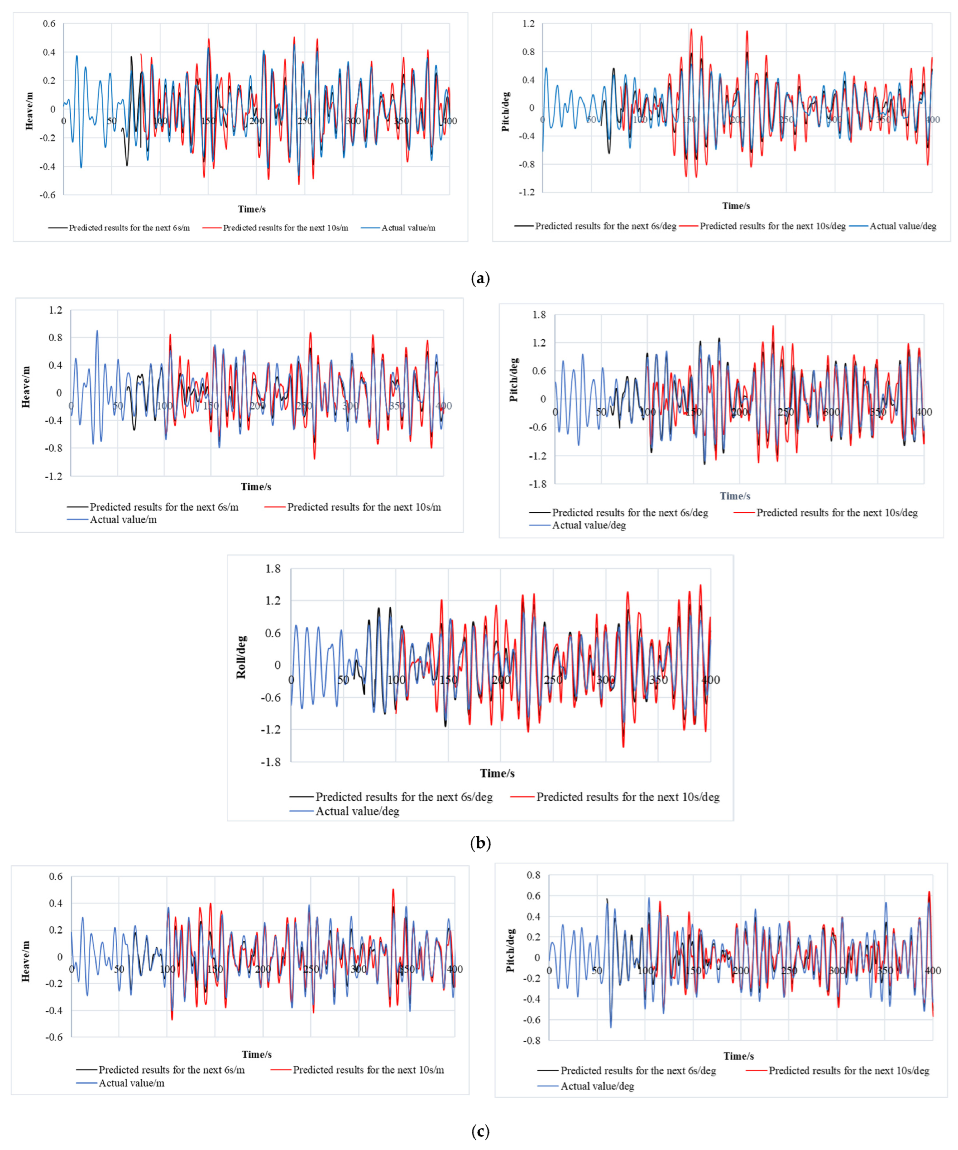
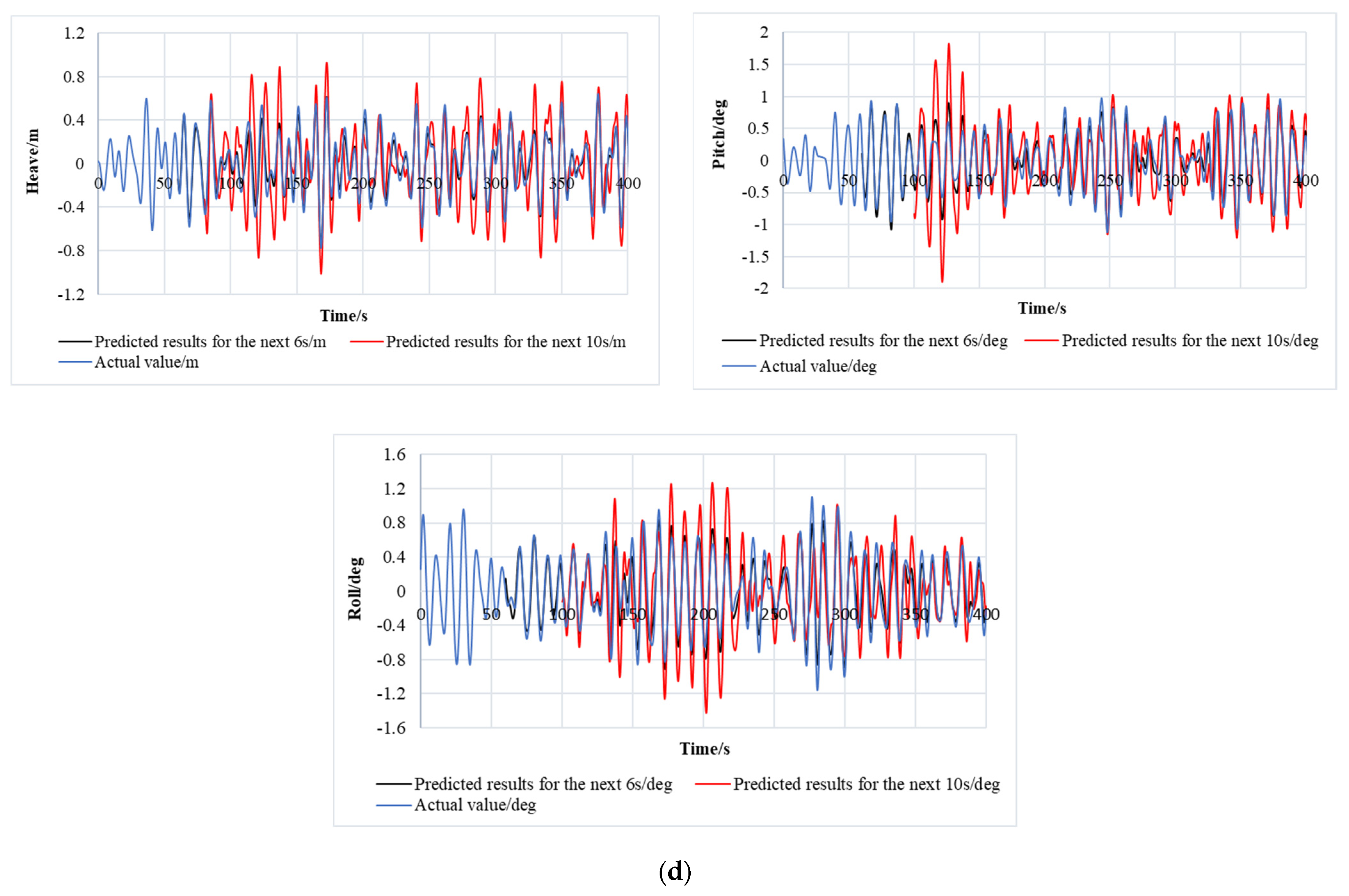
The data comparison of ship motions in random waves is presented in Figure 6, and the error quantification study is detailed in

Table 5. Goodness of fit and loss function.

Case ID	Predictable Time Scale	R2			Loss
		Heave	Pitch	Roll	Heave	Pitch	Roll
Case-I	6 s	0.9315	0.9121	——	6.95 × 10−4	7.09 × 10−4	——
	10 s	0.8894	0.9071	——	7.45 × 10−4	7.37 × 10−4	——
Case-II	6 s	0.8935	0.8911	0.8123	7.45 × 10−4	7.39 × 10−4	8.07 × 10−4
	10 s	0.8784	0.8801	0.8093	7.95 × 10−4	7.97 × 10−4	8.71 × 10−4
Case-III	6 s	0.8375	0.8571	——	7.85 × 10−4	7.79 × 10−4	——
	10 s	0.8084	0.8001	——	7.15 × 10−4	7.27 × 10−4	——
Case-IV	6 s	0.7815	0.7957	0.7436	7.75 × 10−4	7.89 × 10−4	8.52 × 10−4
	10 s	0.7464	0.7460	0.7062	8.45 × 10−4	8.37 × 10−4	8.99 × 10−4

. As it is seen, the predicted results demonstrate a strong agreement with the actual values. All the values of R² are greater than 0.7, which means that the proposed method can capture the characteristics of the ship motions in a random wave. However, some differences can be seen at the peaks of motion corresponding to the predictable time scales of 10 s. Furthermore, the calculating accuracy of the method decreases as the predictable time scale increases. This indicates that as the predictable time scale increases, the complexity of the model increases, and related training volume and training parameters need to be adjusted.

It is noted that the model demonstrates a higher predictive accuracy for heave and pitch compared to roll. This performance discrepancy arises from the use of a unified modeling framework for all degrees of freedom. While efficient, this generalized approach is inherently limited in its capacity to equally capture the distinct dynamic natures of different ship motions, leading to the observed variation in prediction errors.

5. Conclusions

In this work, a real-time prediction method using the LSTM model for ship motions is presented. The effectiveness and feasibility of predicting multiple DOF ship motions are validated through real-time online prediction and transmission using the UDP protocol. The following conclusions can be drawn:

• To evaluate the performance in predicting future motions of the ship, a comparative analysis is carried out between the proposed method and two other neural network models. The results show that the close correspondence between the predicted and actual values validates the efficacy of deep learning, specifically the gated architecture of LSTM networks, in modeling complex nonlinear temporal dynamics, thereby establishing its suitability for ship motion prediction. Moreover, for the proposed method, the training data typically originate from motion records of real-world ships.
• Real-time prediction across multiple time scales was implemented for ship motions in random waves. A key finding is the certain correspondence between the overall trends of the predictions and the actual recorded results. Besides, the prediction accuracy will decrease significantly as the predictable time scale increases. The decrease in accuracy is not only reflected in the overestimation or underestimation of peak value, but also in the frequency dislocation of the time series.
• The primary limitation of the present model lies in the fixed format of input data. The input dimensions must align with the model’s initialization parameters, and the training process depends heavily on GPU acceleration. Furthermore, the CUDA version must be compatible with PyTorch; otherwise, the system defaults to CPU processing, which significantly impedes training speed.

Furthermore, this study still faces certain limitations, such as the generalization capability of the model and practical application. As is known, visualization has been widely employed in the field of ship control. Thus, this study will develop a visualization interface based on source code to facilitate human–computer interaction and apply it to more ship types and sea conditions, thereby achieving greater universality and improved operability.

References

1. Yang, X. Displacement motion prediction of a landing deck for recovery operations of rotary UAVs. Int. J. Contr. Autom. Syst. 2013, 11, 58–64. [Google Scholar] [CrossRef]
2. Huang, L.M.; Duan, W.Y.; Han, Y.; Chen, Y. A review of short-term prediction techniques for ship motions in seaway. J. Ship Mech. 2014, 18, 1534–1542. [Google Scholar]
3. Chen, Z.Y.; Liu, X.Y.; Ji, X.; Gui, H.B. Real-Time Prediction of Multi-Degree-of-Freedom Ship Motion and Resting Periods Using LSTM Networks. J. Mar. Sci. Eng. 2024, 12, 1591. [Google Scholar] [CrossRef]
4. Yu, F.; Cong, W.; Chen, X.; Lin, Y.; Wang, J. Harnessing LSTM for Nonlinear Ship Deck Motion Prediction in UAV Autonomous Landing Amidst High Sea States. In Proceedings of the International Conference on Applied Nonlinear Dynamics, Vibration and Control, Kowloon, Hong Kong, 4–6 December 2023; pp. 820–830. [Google Scholar]
5. Chen, H.; Lu, T.; Huang, J.; He, X.; Sun, X. An Improved VMD–EEMD–LSTM Time Series Hybrid Prediction Model for Sea Surface Height Derived from Satellite Altimetry Data. J. Mar. Sci. Eng. 2023, 11, 2386. [Google Scholar] [CrossRef]
6. Guo, X.; Zhang, X.; Tian, X.; Lu, W.; Li, X. Probabilistic prediction of the heave motions of a semi-submersible by a deep learning model. Ocean. Eng. 2022, 247, 110578. [Google Scholar] [CrossRef]
7. Akaike, H. A Bayesian extension of the minimum AIC procedure Autoregressive model fitting. Biometrika 1979, 66, 237–242. [Google Scholar] [CrossRef]
8. Yumori, I.R. Real time prediction of ship response to ocean waves using time series analysis. In Proceedings of the OCEANS 81, Boston, MA, USA, 16–18 September 1981; pp. 1082–1089. [Google Scholar]
9. Triantafyllou, M.; Athans, M. Real time estimation of the heaving and pitching motions of a ship using a Kalman filter. In Proceedings of the OCEANS 81, Boston, MA, USA, 16–18 September 1981; pp. 1090–1095. [Google Scholar]
10. Soares, C.; Cunha, C. Bivariate autoregressive models for the time series of significant wave height and mean period. Coast. Eng. 2000, 40, 297–311. [Google Scholar] [CrossRef]
11. Panda, J.P. Machine learning for naval architecture, ocean and marine engineering. J. Mar. Sci. Technol. 2023, 28, 1–26. [Google Scholar] [CrossRef]
12. Mateus, B.C.; Mendes, M.; Farinha, J.T.; Assis, R.; Cardoso, A.M. Comparing LSTM and GRU Models to Predict the Condition of a Pulp Paper Press. Energies 2021, 14, 6958. [Google Scholar] [CrossRef]
13. Buestán-Andrade, P.A.; Santos, M.; Sierra-García, J.E.; Pazmiño-Piedra, J.P. Comparison of LSTM, GRU and Transformer Neural Network Architecture for Prediction of Wind Turbine Variables. In Proceedings of the International Conference on Soft Computing Models in Industrial and Environmental Applications, Salamanca, Spain, 5–7 September 2023; pp. 334–343. [Google Scholar]
14. Gers, F.; Schmidhuber, J.; Cummins, F. Learning to Forget: Continual Prediction with LSTM. Neural Comput. 2000, 12, 2451–2471. [Google Scholar] [CrossRef] [PubMed]
15. Bishop, R.; Price, W. On the relationship between “dry modes” and “wet modes” in the theory of ship response. J. Sound Vib. 1976, 45, 157–164. [Google Scholar] [CrossRef]
16. Bishop, R.; Price, W. Hydroelasticity of Ships; Cambridge University Press: New York, NY, USA, 1979. [Google Scholar]
17. Kolway, H.G.; Coumatos, L.M.J. State-of-the-Art in Non-Aviation Ship Helicopter Operations. Nav. Eng. J. 1975, 87, 155–164. [Google Scholar] [CrossRef]
18. Colwell, J.L. Flight Deck Motion System (FDMS): Operating Concepts and System Description; Defence R&D Canada: Dartmouth, NS, Canada, 2004. [Google Scholar]
19. Song, D.L.; Huang, X.Y.; Li, K.; Fu, M.L.; Luo, Y.; Chen, M. Multi-step motion attitude prediction method of USV based on CNN-GRU model. Ship Sci. Technol. 2024, 46, 132–136. [Google Scholar]
20. Abbasimehr, H.; Paki, R. Improving time series forecasting using LSTM and attention models. J. Ambient Intell. Humaniz. Comput. 2022, 13, 673–691. [Google Scholar] [CrossRef]
21. Jaiswal, R.; Singh, B. A Comparative Study of Loss Functions for Deep Neural Networks in Time Series Analysis. In Proceedings of the International Conference on Big Data, Machine Learning, and Applications, Silchar, India, 19–20 December 2021; pp. 147–163. [Google Scholar]
22. Chen, Z.Y.; Du, M.C.; Ji, X.; Liu, X.Y.; Zhao, W.D. Prediction of Ship Future Motions at Different Predictable Time Scales for Shipboard Helicopter Landing in Regular and Irregular Waves. Ships Offshore Struct. 2024, 19, 2172–2180. [Google Scholar] [CrossRef]
23. Chen, Z.Y.; Gui, H.B.; Dong, P.S. Nonlinear time-domain hydroelastic analysis for a container ship in regular and irregular head waves by the Rankine panel method. Ships Offshore Struct. 2019, 14, 631–645. [Google Scholar] [CrossRef]
Figure 1. LSTM operating mechanism flowchart.
Jmse 14 00101 g001
Figure 2. Schematic diagram of future motion prediction using the LSTM model.
Jmse 14 00101 g002
Figure 3. Real-time online prediction and transmission.
Jmse 14 00101 g003
Figure 4. Prediction set normalization.
Jmse 14 00101 g004
Figure 5. R2 corresponding to three neural networks under different sea conditions: (a) Heave; (b) Pitch.
Jmse 14 00101 g005
Figure 6. Data comparison of ship motions in random waves: (a) Predicted values and test sets in Case–I; (b) Predicted values and test sets in Case–II; (c) Predicted values and test sets in Case–III; (d) Predicted values and test sets in Case–IV.
Jmse 14 00101 g006aJmse 14 00101 g006b